VXP: Voxel-Cross-Pixel Large-scale Image-LiDAR Place Recognition

Abstract

Recent works on the global place recognition treat the task as a retrieval problem, where an off-the-shelf global descriptor is commonly designed in image-based and LiDAR-based modalities. However, it is non-trivial to perform accurate image-LiDAR global place recognition since extracting consistent and robust global descriptors from different domains (2D images and 3D point clouds) is challenging. To address this issue, we propose a novel Voxel-Cross-Pixel (VXP) approach, which establishes voxel and pixel correspondences in a self-supervised manner and brings them into a shared feature space. Specifically, VXP is trained in a two-stage manner that first explicitly exploits local feature correspondences and enforces similarity of global descriptors. Extensive experiments on the three benchmarks (Oxford RobotCar, ViViD++ and KITTI) demonstrate our method surpasses the state-of-the-art cross-modal retrieval by a large margin. Our project page is available at: https://yunjinli.github.io/projects-vxp/.

.

1 Introduction

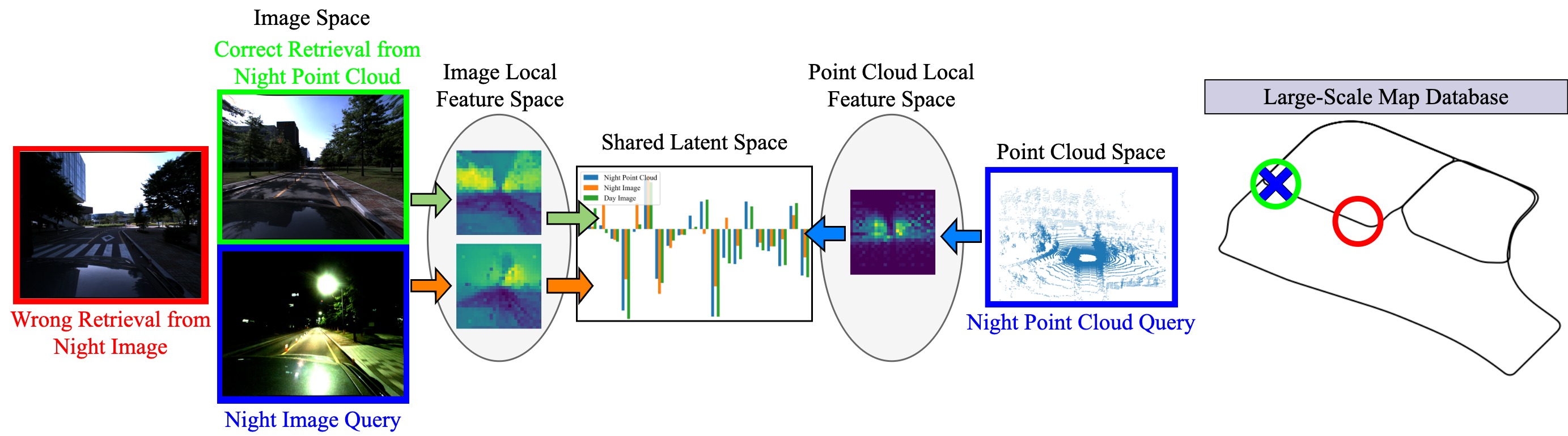
Figure 1: Voxel-Cross-Pixel (VXP) can effectively map data from different modalities into a same shared space, enabling more robust and flexible place recognition. The figure illustrates a case where we have a database recorded at day, and we want to localize the car when driving at night (Note that the blue cross in the map is the current location and the blue boxes are the corresponding data from camera and LiDAR). In this real-world case, uni-modal retrieval (2D-2D) fails because of the variation in light condition. With the aid of VXP, we can potentially use point cloud data, which is robust against environmental changes, to retrieve the correct image (green) in the database (3D-2D). Note that in the latent space, we try to visualize the value for each dimension of a given descriptor (orange: night image, green: day image, blue: night point cloud). We can observe that green and blue bars exhibit more similarity, which demonstrates the advantage in performing 3D-2D cross-modal retrieval.

Global place recognition has been a challenging task for mobile robotics over the decades. Even with the widespread availability of the global position system (GPS), signal outages are still unavoidable, especially in parking spaces or other urban areas where buildings or tunnels can obstruct or divert signals from satellites [37]. These failures are critical for achieving autonomous driving in a city-scale environment and should be handled with onboard devices, such as cameras, LiDARs or radars. The Autonomous Vehicle (AV) sensor suite offers a number of strategies to record data and improve the robustness of global localization. Self-driving car companies like TomTom and HERE are known to actively invest in the development of high-definition maps (HD maps), which are crafted using data collected from various sensors. While a large number of localization solutions has been proposed in the computer vision and robotics community, the majority of them still works within the same modality during map acquisition and operation. The assumption that the data source always provides reliable information limits the applicability of such solutions in cases of sensor malfunctioning or variations in the sensor setup. In the presence of other devices, it underlines the need for more flexible retrieval methods that can be robust against hardware limitations and also exploit the advantages of sensors in different environmental conditions. For instance, cameras are negatively impacted by significant illumination changes, especially at night, while exiting a tunnel or facing a direct sunlight. In contrast, LiDAR can still generate high-quality point cloud maps even in the presence of sudden visual changes. On the other hand, LiDAR scans lack fine-grained details due to their sparse nature, while cameras offer rich and complete depiction of the environment, which is beneficial for large-scale place recognition. Thus, recognizing the potential of cross-modal global place recognition, becomes a noteworthy investment.

The main challenge of localizing images or point clouds using databases from LiDAR or image sensors lies in the huge differences between the images and point clouds, both in terms of raw data and extracted features. LiDAR captures depth information through laser time-of-flight (TOF) measurements, whereas cameras acquire photometric data based on CMOS sensor responses to ambient light. The lack of explicit correlation between these two data modalities complicates their integration. Another observation is that, the point clouds collected from LiDAR is unordered, while images are structured as regular grids. This disparity complicates the development of a single feature extraction method that can effectively process both modalities. To date, only a few approaches have been explored 3D-2D or 2D-3D retrieval solutions. Cattaneo et al. [8] first introduces 2D and 3D feature extraction networks to create a shared embedding space between images and point clouds. $LC^{2}$ [19] proposes to transform image and point clouds into the same 2.5D space for reducing the domain gap. While these methods results in good performance, both approaches ignore a fundamental factor: Accurate local feature correspondences is critical when achieving the cross-modal global place recognition.

To address above problems, we introduce a novel method Voxel-Cross-Pixel (VXP) for image-LiDAR place recognition. In our approach, two separate neural networks are trained to map image data and point cloud maps into the same shared space. The VXP enables the possibility to effectively bridge domain gap between two different sensors, this is resulted from accurate correspondences of local features. Initially, based on the 2D-3D correspondences set by the VXP, we focus on minimizing local descriptor losses, followed by the optimization of global descriptor losses. This comprehensive training paradigm enables the network to effectively capture both fine-grained local details and broader global context, facilitating successful cross-modal mapping. We evaluate our method on the Oxford RobotCar [24], ViViD++ [18] datasets and Kitti Odometry [14] benchmark and demonstrate state-of-the-art cross-modal retrieval.

To summarize, the main contributions of the paper are:

• We propose a novel Voxel-Cross-Pixel (VXP) approach, which establishes voxel and pixel correspondences in a self-supervised manner and brings them into a shared feature space. While learned feature space is agnostic to the input modality, it effectively captures the scene characteristics and allows highly accurate cross-modal place recognition.

• We advocate a two-stage training process, which demonstrates the effectiveness of pre-training the networks on local descriptor similarity constraints and fine-tuning on the global descriptor similarity.

• We establish state-of-the-art performance in cross-modal retrieval on the Oxford RobotCar, ViViD++ datasets and KITTI benchmark, while maintaining high uni-modal global localization accuracy.

2 Related Work

In this section, we first review uni-modal place recognition techniques. We then introduce some fusion-based approaches. Finally, the existing works for cross-modal methods are presented.

Visual and point cloud-based retrieval.

Uni-modal place recognition methods operate within one sensor type and aim to find the closest query match in a database. Most widely researched modalities are visual and LiDAR-based, while other types such as radar recently have received attention from the community [5]. Traditional image-based approaches, such as bag-of-words [13], represent different places with a visual vocabulary of quantized local descriptors [26]. In recent years, Convolutional Neural Network (CNN)-based methods have gained popularity for their expressiveness and enhanced robustness. Arandjelović et al. introduced NetVLAD [4], a CNN-based approach that encodes RGB images into dense feature maps and learns to effectively aggregate these features into a global descriptor. CosPlace [6] explored to perform the retrieval as a classification task. Recent works [1, 2] proposed to process the features extracted by a CNN with a Conv-AP layer or a Feature-Mixer. As for LiDAR-based place recognition, Uy et al. proposed PointNetVLAD [33], in which they employed PointNet [27] to extract features from a point cloud map and then aggregate them into a global descriptor using a subsequent NetVLAD layer. LPD-Net was introduced by Liu et al. [22], in which they proposed an adaptive local feature extraction module to extract local features and the graph-based aggregation module. SOE-Net [38] first introduces orientation encoding into PointNet and a self-attention unit to generate a robust 3D global descriptor. Furthermore, various methods [41, 11] explored the integration of different transformer networks to learn long-range contextual relationships. In contrast, Minkloc3D [16] employed a voxel-based strategy to generate a compact global descriptor. However, the voxelization methods inevitably suffer from information loss due to the quantization. Recent CASSPR [36] thus introduced a hierarchical cross attention transformer, combining both the advantages of voxel-based strategies with the point-based strategies. Text2Loc [37] achieved the 3D localization based on textual descriptions. In this paper, our work brings the best practices of 2D image and 3D point cloud communities together into a coherent framework that can achieve state-of-the-art performance in cross-modal retrieval.

Fused-Modal Place Recognition.

As mentioned earlier, LiDAR-based methods are more robust to variations in illumination and appearance when compared to the vision-based approaches. However, obtained scans are limited in capturing fine details of the observed scenes, which could be beneficial in localization tasks. To this end, researchers have started exploring the possibility of fusing image and LiDAR data for the place recognition task. Pan et al. proposed a method called CORAL [25], in which point cloud data is converted into an elevation image in order to perform further fusion. MinkLoc++ [17], on the other hand, employed a late fusion technique, processing point cloud and image data separately and performing fusion at the final stage. While our approach relies on having both image and LiDAR data available during training, due to the chosen architecture with two independent branches we are capable of dealing with a single stream data during inference, which enables cross-modal retrieval.

Cross-Modal Place Recognition.

Only few studies have been proposed to tackle cross-modal registration such as 2D-3D re-localization [21, 30, 34, 12]. These methods primarily concentrate on accurately localizing a camera within a given point cloud map by matching image keypoints to 3D points. Once correspondences are established, a transformation can be computed using the Perspective-n-Points (PnP) algorithm. Although these approaches are not explicitly designed for the place recognition task, the concept of matching from the 2D scene captured by the camera to the 3D local structure recorded by LiDAR is shown to be promising and beneficial for the cross-modal retrieval methods.

To the best of our knowledge, there are only a few existing approaches that specifically address cross-modal place recognition. The work by Cattaneo et al. [8] was first to introduce the task and propose a data-driven method, where they trained two networks for encoding images and point cloud maps respectively in a teacher-student training manner. Initially, they trained image teacher using the triplet loss function [31]. Subsequently, they trained point cloud network to bring point embeddings into the shared latent space. In our work, we leverage a similar paradigm of the teacher-student training, however we further enhance global description using local information and obtain state-of-the-art cross-modal performance. The $LC^{2}$ approach, proposed by Lee et al. [19], presented an alternative method for cross-modal retrieval, where the domain gap was bridged by pre-processing sensor data and transforming it into the same data representations. Specifically, they converted both types of data into the 2.5D space, where RGB images were turned into disparity maps using depth network [35] and LiDAR point clouds were transformed into range images. A self-supervised pre-training scheme [20] was employed on the encoders, enabling the networks convergence. In comparison, our method directly handles input raw data and does not require computationally demanding pre-processing steps, which would be more favorable for on-board devices.

3 Method

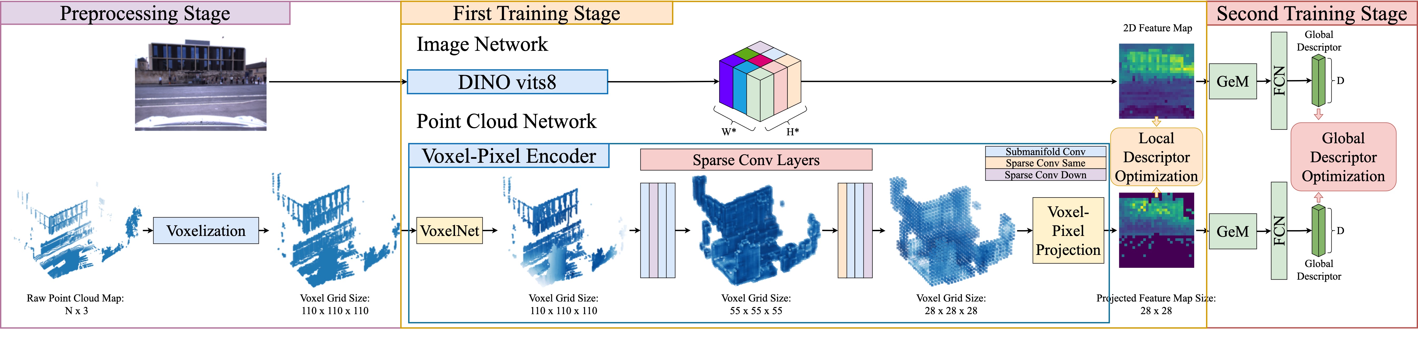
Figure 2: The overview of our VXP. VXP consists of three stages: Preprocessing Stage, First Training Stage (local descriptor optimization), and Second Training Stage (global descriptor optimization). The two networks operate independently during inference. The objective is to map different data into a same shared latent space, so that the distance (e.g. L2) can be computed between the global descriptors from point cloud and image. Image Processing: An image is first processed by DINO ViTs-8 encoder to generate a 2D feature map. Finally, the GeM and the Fully-Connected Layer compress the feature map into a global descriptor. Point Cloud Processing: The point cloud map $\textbf{P}\in\mathbb{R}^{N\times 3}$ is processed into the voxel grid. The voxel grid $\textbf{V}=\{\textbf{v}_{i}\in\mathbb{R}^{M\times 3},\textbf{c}_{i}\in\mathbb{R}^{3}\}_{1,2,...,T}$ is then fed into VoxelNet [40] to encode the feature for each voxel. Afterwards, series of 3D sparse convolution are applied to extract more refined 3D feature map. Finally, the 3D feature map would be projected to 2D by the Voxel-Pixel Projection module, and the global descriptor is generated by the following GeM and Fully-Connected Layer.

In this section, we introduce our cross-modal place recognition approach in detail. VXP pipeline is shown in Fig. 2. We design two separate networks that map image and point cloud into the same shared latent space. Each network would learn to generate a global descriptor which is expected to encode all the necessary information for the given input data. Mathematically, we can formulate our approach with Eq. 1. The function $f$ represents the image network, while $g$ characterizes the point cloud network.

$$f: \quad\mathbb{R}^{H\times W\times 3} \rightarrow\mathbb{R}^{D}$$ (1)

$$g: \quad\mathbb{R}^{N\times 3} \rightarrow\mathbb{R}^{D}$$

3.1 Image Network

The image network architecture comprises two components: (1) the DINO ViTs-8 encoder and (2) a global pooling layer (GeM + FCN) as illustrated in Fig. 2. In the initial phase, the raw RGB image, denoted as $I\in R^{H\times W\times 3}$, is processed by the DINO ViTs-8 encoder $f^{enc}:R^{H\times W\times 3}\rightarrow R^{H^{*}\times W^{*}\times D}$. This operation yields 2D features, which are also recognized as local image feature descriptors. Subsequently, these generated image features are passed through the global pooling layer $f^{pool}:R^{H^{*}\times W^{*}\times D}\rightarrow R^{D}$, resulting in the creation of a global image descriptor.

3.2 Point Cloud Network

Dealing with raw point cloud data, which typically consists of thousands of points, can pose a significant computational challenge. To tackle this problem, we leverage point cloud grouping techniques as a means of mitigating computational costs, which has also been shown to effectively capture local structures [28]. Consequently, we deploy voxelization method [40] to transform the raw point cloud data $\textbf{P}\in\mathbb{R}^{N\times 3}$ into a voxel grid $\textbf{V}=\{\textbf{v}_{i}\in\mathbb{R}^{M\times 3},\textbf{c}_{i}\in\mathbb{R}^{3}\}_{1,2,...,T}$, where $T$ is the number of non-empty voxels and $M$ represents the number of points within a voxel.

In Fig. 2, the initial voxel feature $\textbf{v}\in\mathbb{R}^{M\times 3}$ aggregates information from $M$ raw point coordinates contained within the voxel boundaries. We use VoxelNet [40] to extract more detailed descriptor for each voxel $\textbf{v}\in\mathbb{R}^{M\times 3}\quad\rightarrow\quad\mathbb{R}^{D}$. Finally, we perform a series of sparse 3D convolutions [39] to generate a compact 3D feature map of size $28\times 28\times 28$, namely $\textbf{V}_{out}$, as formulated in Eq. 2. The $\textbf{v}_{i}^{out}$ represents a local descriptor of a single voxel in the output voxel grid, while $\textbf{c}_{i}^{out}$ denotes the coordinate of this voxel within the voxel grid. Here, $\textbf{c}_{i}^{out}$ is defined with respect to the voxel grid coordinate frame $\{\mathcal{V}\}$. Sparse convolutions allow us to aggregate spatial information from neighboring voxels in a hierarchical fashion, which allows to capture long-distance relations.

$$\textbf{V}_{out}=\{\textbf{v}_{i}^{out}\in\mathbb{R}^{D^{*}},\textbf{c}_{i}^{out}\in\mathbb{R}^{3}\}_{1,2,...,28^{3}}$$ (2)

In order to bridge the domain gap between point cloud and image, we introduce simple yet effective Voxel-Pixel Projection module. This module projects voxels onto the image plane using the pinhole camera model. However, it’s important to note that the voxel coordinates are defined within the voxel grid coordinate system denoted as $\{\mathcal{V}\}$. Therefore, we formulate the coordinate transformation between the voxel grid coordinate frame $\{\mathcal{V}\}$ and the point coordinate frame $\{\mathcal{P}\}$ in Eq. 3.

$$\begin{bmatrix}X_{i}\\ Y_{i}\\ Z_{i}\end{bmatrix}^{\mathcal{P}}=\begin{bmatrix}v_{x}&0&0\\ 0&v_{y}&0\\ 0&0&v_{z}\end{bmatrix}\textbf{c}_{i}^{out}+\begin{bmatrix}v_{x}/2+x_{min}\\ v_{y}/2+y_{min}\\ v_{z}/2+z_{min}\end{bmatrix}$$ (3)

Note that $(v_{x},v_{y},v_{z})$ is the dimension of the output voxel grid and the lower bound of the point cloud range is represented as $(x_{min},y_{min},z_{min})$. After transforming the voxel coordinates to $\{\mathcal{P}\}$, a rotation is applied to align the axes with the camera coordinate axes convention (x-right, y-down, and z-forward). Finally, we project the transformed voxels into the image plane using the pinhole camera model in Eq. 4 in order to obtain the final feature map and allow to establish local descriptor constraints as demonstrated in Fig. 3.

$$\lambda\begin{bmatrix}u_{i}\\ v_{i}\\ 1\end{bmatrix}=\begin{bmatrix}f_{x}&0&c_{x}\\ 0&f_{y}&c_{y}\\ 0&0&1\end{bmatrix}\begin{bmatrix}0&-1&0\\ 0&0&-1\\ 1&0&0\end{bmatrix}\begin{bmatrix}X_{i}\\ Y_{i}\\ Z_{i}\end{bmatrix}^{\mathcal{P}}$$ (4)

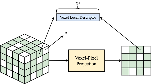
(a) $\phi$ represents “empty” as the 3D feature maps are sparse. Note that the voxel local descriptor is the $\textbf{v}_{i}^{out}$ introduced in Eq. 2

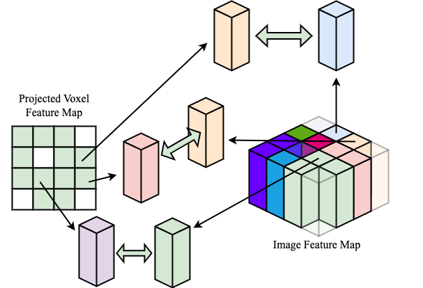
(b) The projected voxel feature map $\mathcal{M}_{V}$ is in sparse data structure. The corresponding descriptor can be retrieved by the 2D index $(u_{i},v_{i})$. The local descriptor loss can be computed by all the non-empty descriptors in the projected voxel feature map.

Figure 3: (a): the illustration of the Voxel-Pixel Projection module. (b): the illustration of local descriptor optimization.

Finally, the new projected feature map would be fed into the global pooling layer (GeM + Fully-Connected Layer) to extract the global descriptor to enable the second stage optimization, as described in the following sections.

3.3 Teacher-Student Training Paradigm

Inspired by effectiveness of the training framework in [9], we perform teacher-student distillation for the image-LiDAR retrieval. The approach entails two sequential steps: initially, we train the image network considered to be the teacher network by triplet loss function [31]: Each triplet consists of three components: an anchor image denoted as $I^{a}_{i}$, a positive image $I^{p}_{i}$ closely related to the anchor image’s location, and a negative image $I^{n}_{i}$ positioned far away from the anchor image. The loss function is defined as follows:

$$\mathcal{L}_{HPHN}=\sum_{I_{i}^{a},I_{i}^{p},I_{i}^{n}\in\cal{B}}[ Max(d(f(I_{i}^{a}),I_{i}^{p}))$$ (5)

$$- Min(d(f(I_{i}^{a}),I_{i}^{n}))+m]_{+}.$$

Note that $d(.)$ is the distance function, $f(.)$ is the image branch model, $m$ is the margin, and $[.]_{+}$ means $Max(0,[.])$. In order to train more efficiently, we try to find the hardest positive sample and the hardest negative sample of the anchor within the mini-batch $\mathcal{B}$ when computing the triplet loss. Subsequently, we proceed to train a separate network for the point cloud branch, namely the student network, which essentially endeavors to bridge the dissimilarity with the features produced by the teacher network.

3.4 Two-Stage Descriptor Training

To the best of our knowledge, our work is the first in advocating two-stage global descriptor training, which firstly establishes close resemblance in local descriptors and, secondly, transfers the knowledge while training for the global descriptor. Two stages are shown in Fig. 2. During the local descriptor optimization phase shown in Fig. 3(b), we utilize the projected voxel coordinates $(u_{i},v_{i})$ as indices to retrieve the corresponding local descriptors from the image feature map. Once they are retrieved, we can apply the local descriptor loss function as in Eq. 6.

$$\mathcal{L}_{local}=\sum_{(u_{i},v_{i})\in\mathcal{M}_{V}}\rho(\mathcal{M}_{V}(u_{i},v_{i})\cdot d_{i},\mathcal{M}_{I}(u_{i},v_{i}))$$ (6)

The projected voxel feature map is denoted as $\mathcal{M}_{V}$, the image feature map is $\mathcal{M}_{I}$, and $\rho$ is the cost function. We also take care of collisions, when multiple voxels are projected to the same pixel, by weighting descriptors with their voxels’ inverse depths $d_{i}$. This way we give preference to the voxels that are closer to the camera.

In the second stage, we take the weights of the model trained in the first stage using local descriptor loss (Eq. 6) and fine-tune global descriptors with

$$\mathcal{L}_{global}=\sum_{i}\rho(f(I_{i}),g(P_{i})),$$ (7)

where $I_{i}$ denotes as the image, $P_{i}$ denotes as the point cloud, $f(.)$ and $g(.)$ refers to the teacher and student network respectively, and $\rho$ is the cost function.

4 Experiments and Results

4.1 Implementation Details

Our implementation is built in the PyTorch framework. When using ViT as the image encoder, we resize the image to $224\times 224$, in other cases to $240\times 320$. During training of the teacher network, positive pairs are chosen from images that are within 10 meters, while the negative pairs are defined from samples that are more than 25 meters away as [19]. We set the margin of the triplet loss function to 0.3. To handle situations where zero-triplets occur, we employ a strategy of gradually increasing the batch size if the proportion of zero-triplets exceeds 30% of the original batch size. The branch expansion rate is configured at 1.4, and the maximum batch size is set to 256. To train the student network we adopt the following voxelization parameters: point cloud boundaries range is $x:[0,44],y:[-22,22],z:[-4,18]$, voxel dimensions are set to $[v_{x},v_{y},v_{z}]=[0.4,0.4,0.2]$. This would allow us to have a final voxel grid with size (110, 110, 110). Both the cost function $\rho$ in $\mathcal{L}_{local}$ and $\mathcal{L}_{global}$ are chosen as smooth L1 loss to ensure robustness to outliers. Adam optimizer and LambdaLR learning rate scheduler are utilized in our training pipeline.

4.2 Datasets

Oxford RobotCar Dataset. We utilize the Oxford Robotcar benchmark [24] for evaluation, where the same trajectory was traveled over a year in different times of the day and seasonal conditions. We generate data samples following the same protocol as conducted by Cattaneo et al. [9], where image is recorded every five meters and the corresponding point cloud map is constructed by concatenating the subsequent 2D LiDAR scans. The dimension of the point cloud map is expected to be 50 meters along all axes. The four test regions are excluded from the training dataset as per [33].

ViViD++ Dataset. Additionally, we assess the performance of our model on the ViViD++ dataset [18], which consists of driving and handheld sequences and covers 3D LiDAR, visual and GPS data. In the scope of our work, we are mainly interested in the urban data, which contains sensor measurements recorded during a day, evening and night. We follow the training procedures proposed by Lee et al. [19] where only the day1 sequences are used for training, while performing evaluation with day2 and night sequences.

KITTI Odometry Dataset. We further test the generalization capability of our VXP on the KITTI Odometry benchmark [14], which contains sequences with LiDAR scans, images, and ground-truth poses.

4.3 Quantitative Results

Oxford RobotCar. We adhere to the evaluation metric employed by Cattaneo, in which we select each pair of distinct runs from 23 sequences as query and database. The query contains samples only from the four excluded regions as per [33], while database consists of samples from the entire trajectory. Finally, the average of the recall is computed for all the pairs. In Tab. 1, we compare our model with the two existing cross-modal approaches for both the uni-modal global localization, specifically image-only (2D-2D) and point cloud-only (3D-3D), and the cross-modal localization, where image serves as a query and point cloud as a database (2D-3D) and vice-versa (3D-2D). Our method outperforms other baselines on cross-modal place recognition and demonstrates the best performance in the uni-modal retrieval thanks to the two-stage descriptor optimization as presented in 3.4 and verified in the ablation studies 5.1. Fig. 4 shows average recall for different top@K values against our implementation of Cattaneo et al. [9] method. Our method demonstrates higher accuracy than the baseline, which validates consistency of our method.

Table 1: Uni- and cross-modal Recall@1% from Oxford RobotCar Dataset [24].

	2D-2D	3D-3D	2D-3D	3D-2D
Cattaneo [9]	96.63	98.43	77.28	70.44
$LC^{2}$ [19]	84.14	82.98	81.23	73.84
VXP (Ours)	98.79	98.84	84.39	76.93

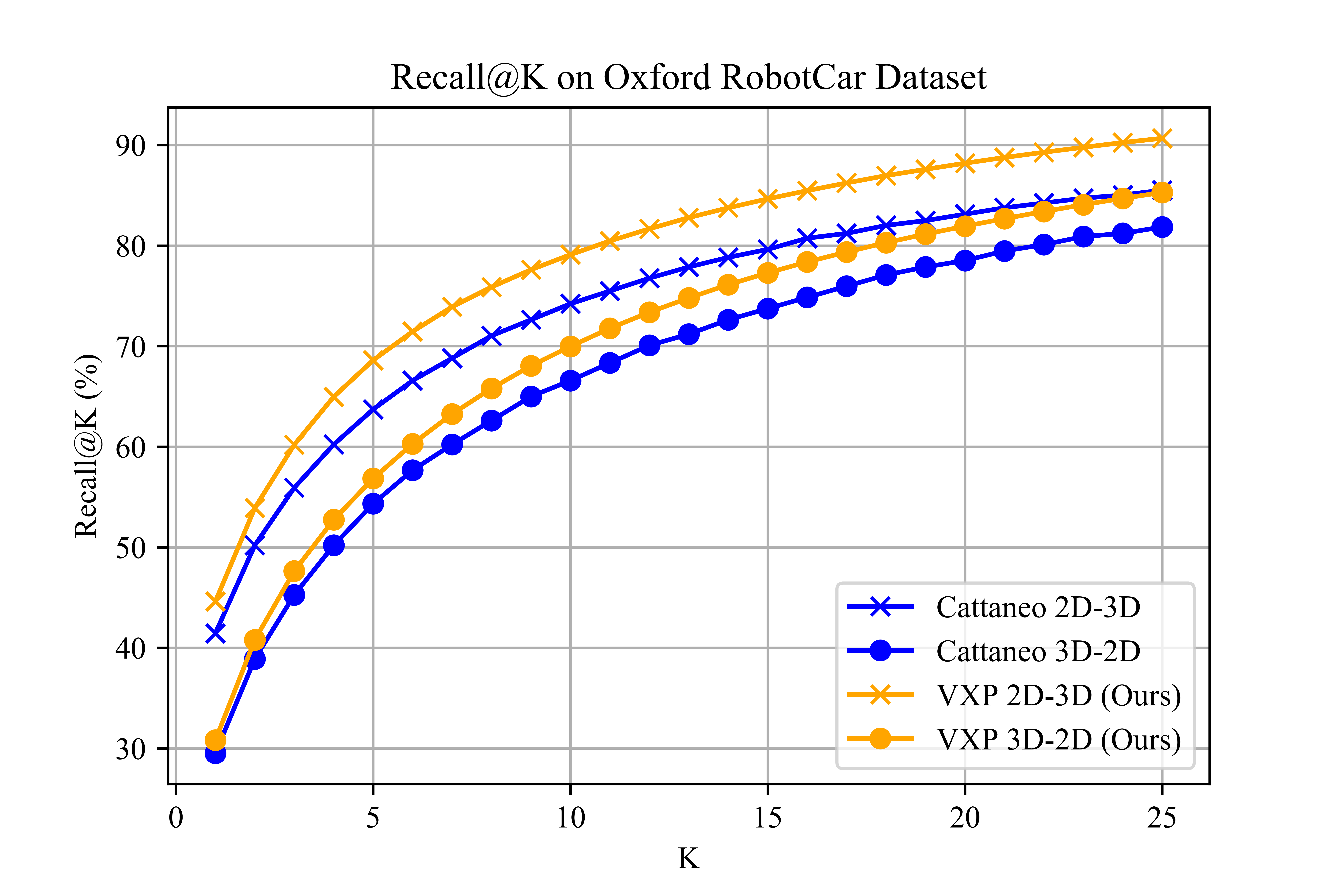
Figure 4: Recall for up to K = 25 retrieved places. VXP consistently demonstrates superior cross-modal retrieval accuracy. Note that the values of $LC^{2}$ is not available in their publication.

ViViD++. We further evaluate our model on the ViViD++ dataset and compare the results of different approaches on day1-day2 sequences in Tab. 2. Note that day1-day2 represents query from day1 sequences and database using day2 sequences. As the code from [9] is not publicly released, we have implemented the approach with the authors’ help to the best of our abilities. Overall, we outperform the other baselines [9, 19] on the cross-modal place recognition and perform on par with [9] on uni-modal retrieval task.

We also evaluate our method on the night-day retrieval, where database map is recorded in the day and queries are obtained at night. Our VXP is able to tackle this issue by incorporating information from the LiDAR scans that are not affected by insufficient lighting conditions. The results are shown in Tab. 3. VXP outperforms $LC^{2}$ and the model by [9] on the 3D-2D place recognition task and shows highly accurate results based on the top selected retrieval candidate. Specifically, for the Top@1 average recall metric we achieve a boost in performance by a large margin ($\sim 16\%$ improvement). As shown in Tab. 3, image retrieval (2D-2D) struggles in the challenging scenarios of the night-day retrieval, while cross-modal recognition is capable to offer more accurate place recognition performance across all baselines.

Table 2: Recalls of day1-day2 on the ViViD++ dataset. Note that the average recall is computed from city day1$-$city day2 and campus day1$-$campus day2.

Recall@1	2D-2D	3D-3D	2D-3D	3D-2D
$LC^{2}$ [19]	69.21	58.06	60.87	51.77
Cattaneo’s [9]	93.39	90.97	87.58	78.58
VXP (Ours)	91.04	92.25	91.68	88.93
Recall@1%	2D-2D	3D-3D	2D-3D	3D-2D
$LC^{2}$ [19]	96.85	96.06	95.98	94.57
Cattaneo’s [9]	99.83	99.90	99.63	98.62
VXP (Ours)	99.70	99.73	99.66	99.73

Table 3: 2D-2D and 3D-2D Recalls of night-day2 on ViViD++ dataset. Note that this is the average recall computed from city night$-$city day2 and campus night$-$campus day2. Here we can clearly see with the help of cross-modal approach, we can still maintain the performance.

2D-2D	$LC^{2}$ [19]	Cattaneo’s [9]	VXP (Ours)
Recall@1	0.78	2.24	10.16
Recall@1%	5.53	10.08	24.12
3D-2D	$LC^{2}$ [19]	Cattaneo’s [9]	VXP (Ours)
Recall@1	49.38	56.87	72.40
Recall@1%	93.39	94.84	96.84

KITTI Odometry Benchmark. The results are shown in Tab. 5. Unlike the evaluation protocol followed by [36, 10, 23] for LiDAR-based place recognition, we propose our own evaluation protocol for cross-modal place recognition inspired by the one used by Oxford RobotCar. We train the model on sequences 03, 04, 05, 06, 07, 08, 09, 10. For testing we select 4 regions from sequences 00 and 02 and include the remaining parts of the trajectory in the training data. Notably, none of the sequences traverses the same place, so we test our model on completely unseen regions to demonstrate generalisation capability of our method. We provide further training details in the supplementary. As demonstrated in Tab. 5 our method outperforms the baseline [9] by a large margin, achieving double accuracy on Top@1 for both 2D-3D and 3D-2D retrieval tasks. Since the full code for the $LC^{2}$ is not publicly available, we cannot provide comparison on this benchmark.

Table 4: Cross-modal recalls of the Kitti Odometry (00). Our model achieves on average 2$\times$ improvement for 2D-3D and 3D-2D Recall@1.

Recall@1	2D-3D	3D-2D
Cattaneo’s [9]	22.82	16.60
VXP (Ours)	47.16	30.01
Recall@1%	2D-3D	3D-2D
Cattaneo’s [9]	71.72	56.09
VXP (Ours)	81.74	65.21

Table 5: Cross-modal recall@1 and 1% with the presence of Two-stage Descriptor Optimization from Oxford RobotCar Dataset.

	One-stage	Two-stage
2D-3D@1	41.31	44.60
3D-2D@1	30.19	30.81
2D-3D@1%	81.51	84.39
3D-2D@1%	74.74	76.93

5 Ablation Studies

5.1 Multi-stage Student Network Training

We compare the performance with and without our proposed Two-stage Descriptor Optimization in Tab. 5. The proposed optimization technique facilitates the model in bridging the domain gap between image and point cloud.

5.2 Teacher Network Selection

In the preceding section, we conducted extensive testing with various image encoders and pooling layers, and the results are summarized in table Tab. 6. Overall, it is evident that DINO [7] stands out as the most favorable choice for the image encoder. Concerning the pooling layers, GeM [29] seems to perform slightly better than NetVLAD [4]. Based on the experiments, it is clear that the combination of DINO + GeM + FCN yields the most optimal results. Additionally, we evaluated the performance of an off-the-shelf DINO model because it’s been demonstrated to be capable of addressing a wide range of tasks [3]. However, the performance is quite poor (only 59.47% on 2D-2D Recall@1 as per evaluation in Tab. 1) since it was not trained for the place recognition task. In Fig. 5 visually illustrates the noticeable changes in the attention map with and without fine-tuning on Oxford RobotCar dataset [24]. We can see the buildings have higher attention scores in general after fine-tuning.

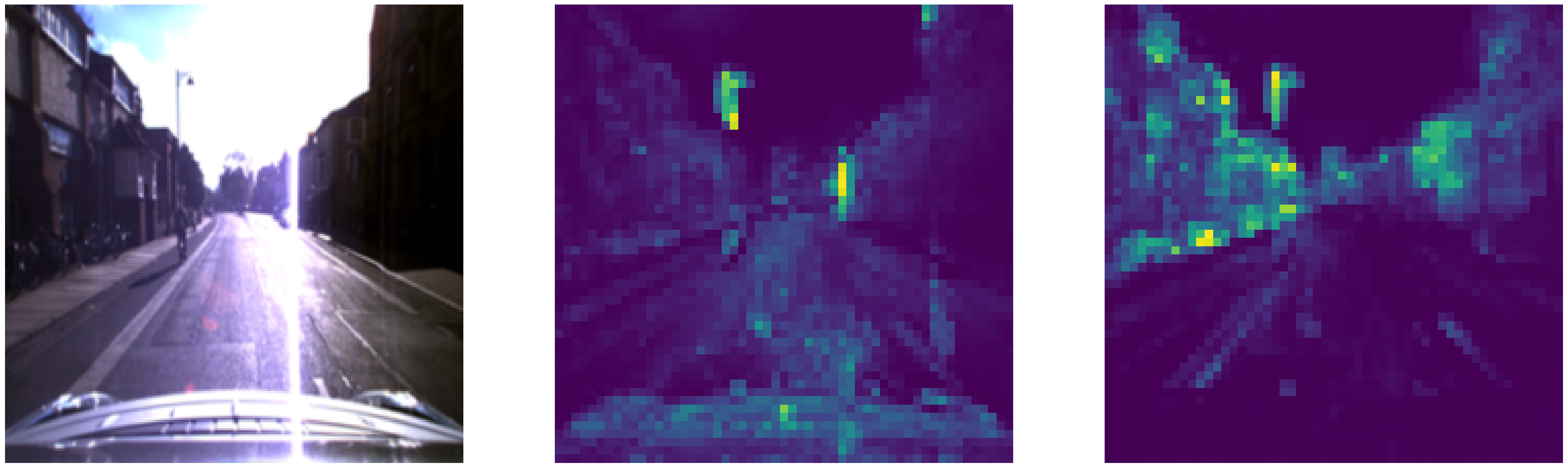
Figure 5: The visualization of attention maps. The original RGB image (left), the attention map generated by DINO’s ViTs-8 from its 11th layer without fine-tuning (middle), and the attention map with fine-tuning (right) on Oxford RobotCar dataset [24].

Table 6: The comparison of the different combinations of image encoder and pooling layer. Note that V16 represents VGG16 [32], R18 is ResNet18 [15], Dino is DINO’s ViTs-8 [7], N means NetVLAD [4], G refers to GeM [29], L means fully-connected layer. Note that the evaluation was obtained by using both query and database generated with 20 meters interval, as this enable faster runtime.

2D-2D	Recall@1	Recall@1%
V16+N+L	80.4122	91.5839
V16+G+L	81.6639	92.7453
R18+N+L	77.2257	90.3156
R18+G+L	78.6817	91.0627
Dino+N+L	85.2995	94.8824
Dino+G+L	85.2849	94.9596

5.3 Qualitative Evaluation for VXP

As we have shown in Sec. 4.3, VXP achieved state-of-the-art performance, prompting our interest in delving deeper into the underlying mechanisms that contribute to its success. We explore the correlation between the attention map of the RGB image and the inverse depth map of the projected voxels in Fig. 6. As we introduced in Sec. 3, our goal is to mitigate the domain gap between the point cloud and the image by projecting the 3D feature map into a 2D feature map. Given that the subsequent pooling layer exclusively considers voxels projected within the image, it becomes crucial to analyze and compare the patterns present in these two distinct feature maps. Since our focus is on place recognition, structures such as buildings carry greater significance, resulting in higher attention scores in those regions. Notably, the projected voxels exhibit a similar pattern, which proves advantageous for optimizing the relevant sections of the feature map during the optimization process.

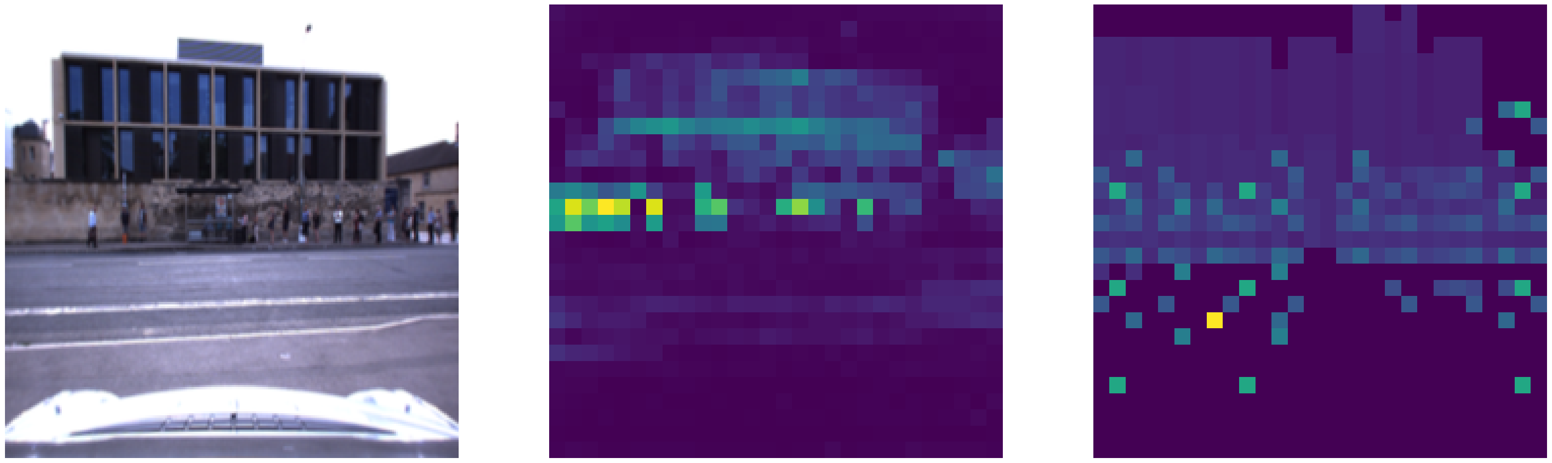
Figure 6: The visualization of attention map (middle) with corresponding RGB image (left), and the inverse depth map (right) generated from the corresponding point cloud.

5.4 Training and Inference Efficiency

We evaluate model inference time using a single RTX3080 and preprocessing time with Intel i7-12700. (Depth image generation is done on GPU) Our VXP takes 7 ms and 18 ms to obtain a global descriptor for an image and a point cloud respectively, while $LC^{2}$ [19] achieves it in 17 ms and 53 ms due to expensive preprocessing step of depth image generation and point cloud to range image conversion. 2D and 3D networks of VXP have 21.7M (87.2MB) and 5.9M (23.6MB) parameters respectively. Our model is fast and compact to run as part of a real-time system. Notably, the reference map can be encoded offline.

5.5 Discussion about Domain Bridging

Existing methods in cross-modal place recognition share a common theme - employing modules to bridge the domain gap between different data modalities. For instance, in $LC^{2}$ [19], this is achieved by processing RGB images and the point clouds into the disparity maps and the range images. By transforming 2D and 3D data into 2.5D proves to be beneficial for cross-modal place recognition. However, this transformation sacrifices uni-modal performance due to information loss during preprocessing of raw data. Similarly, in the method proposed by Cattaneo et al. [9], they compress 3D feature maps into 2D to bridge the modality gap but encounter challenges in properly setting correspondences for supervision. In contrast, our method directly operates on both point cloud data and RGB images. We establish voxel and pixel correspondences and brings their feature spaces together in a self-supervised manner.

6 Conclusion

We proposed VXP for image-LiDAR place recognition. VXP makes use of a novel 3D-to-2D projection module specifically designed to establish local feature correspondences, effectively bridging the domain gap between the LiDAR and cameras. Additionally, we proposed a two-stage descriptor optimization pipeline, a key factor in overcoming sub-optimal results observed in prior methods. Notably, our approach directly works on raw data without any sophisticated preprocessing pipelines. This distinct characteristic enables faster inference, crucial for real-world applications. Experimental evaluations demonstrate that VXP provides a new state-of-the-art performance and excellent generalization ability on image-LiDAR retrieval. Future work will explore its integration into the Simultaneous Localization and Mapping (SLAM) pipelines and real robots.

Appendix 0.A Supplementary Material

In the supplementary we provide further details of the coordinate system convention in Sec. 0.A.1, evaluation procedure on the KITTI Odometry dataset Sec. 0.A.2, and some qualitative results Sec. 0.A.3. We report some failure cases in Sec. 0.A.4 and visualize cross-modal local correspondences in latent space in Sec. 0.A.5. Finally, we shall release the code upon acceptance to inspire further work in the direction of image-LiDAR place recognition.

0.A.1 Coordinate Frames

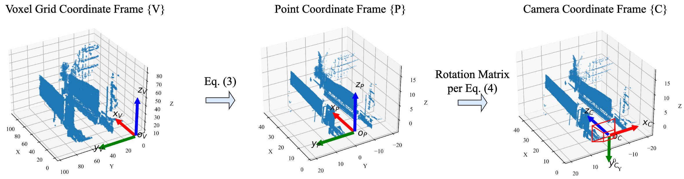
Figure 7: Illustrations of voxel grid coordinate frame $\mathcal{\{V\}}$ (left), point coordinate frame $\mathcal{\{P\}}$ (middle), and camera coordinate frame $\mathcal{\{C\}}$ (right). Note that once the points are transformed to $\mathcal{\{C\}}$, we can apply pinhole camera projection to project points to pixel coordinate frame.

In Sec. 3.2 (main), we introduce Voxel-Pixel Projection module along with the associated coordinate transformations. Accordingly, in Fig. 7, we provide a comprehensive illustration of the operational coordinate frames $\mathcal{\{V\}}$, $\mathcal{\{P\}}$, and $\mathcal{\{C\}}$ and demonstrate the transformations between them as per Eq. 3 and Eq. 4.

0.A.2 Training / Testing Setup in KITTI

In Tab. 5 of Sec. 4.3 (main), we present the evaluation on the KITTI Odometry Benchmark [14]. Our evaluation protocol draws inspiration from the methodology employed in the Oxford RobotCar dataset [24]. As shown in Fig. 8, we define non-overlapping regions in KITTI sequences 00 and 02 and exclude samples from these regions during the training process. This way we ensure that the model is tested on unseen scenes during the testing phase. Throughout the training process, samples from the test regions in sequence 02 are utilized for validation, and we select the best model based on the validation. During testing, queries are drawn from the test regions in sequence 00, while the entire trajectory from sequence 00 serves as the database. Notably, we exclude the sample corresponding to the query from the list of retrieval candidates.

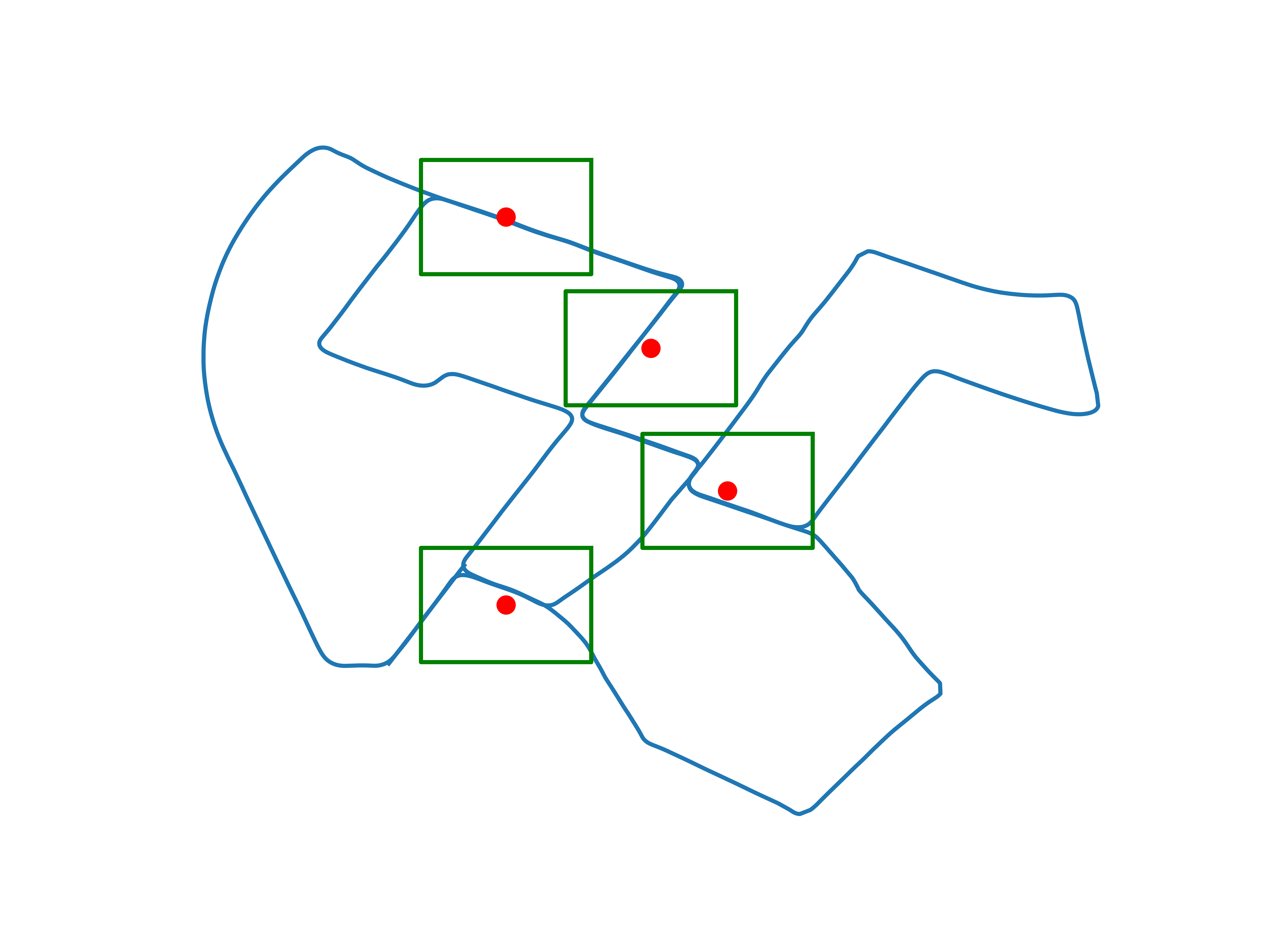
(a) Test regions in KITTI sequence 00.

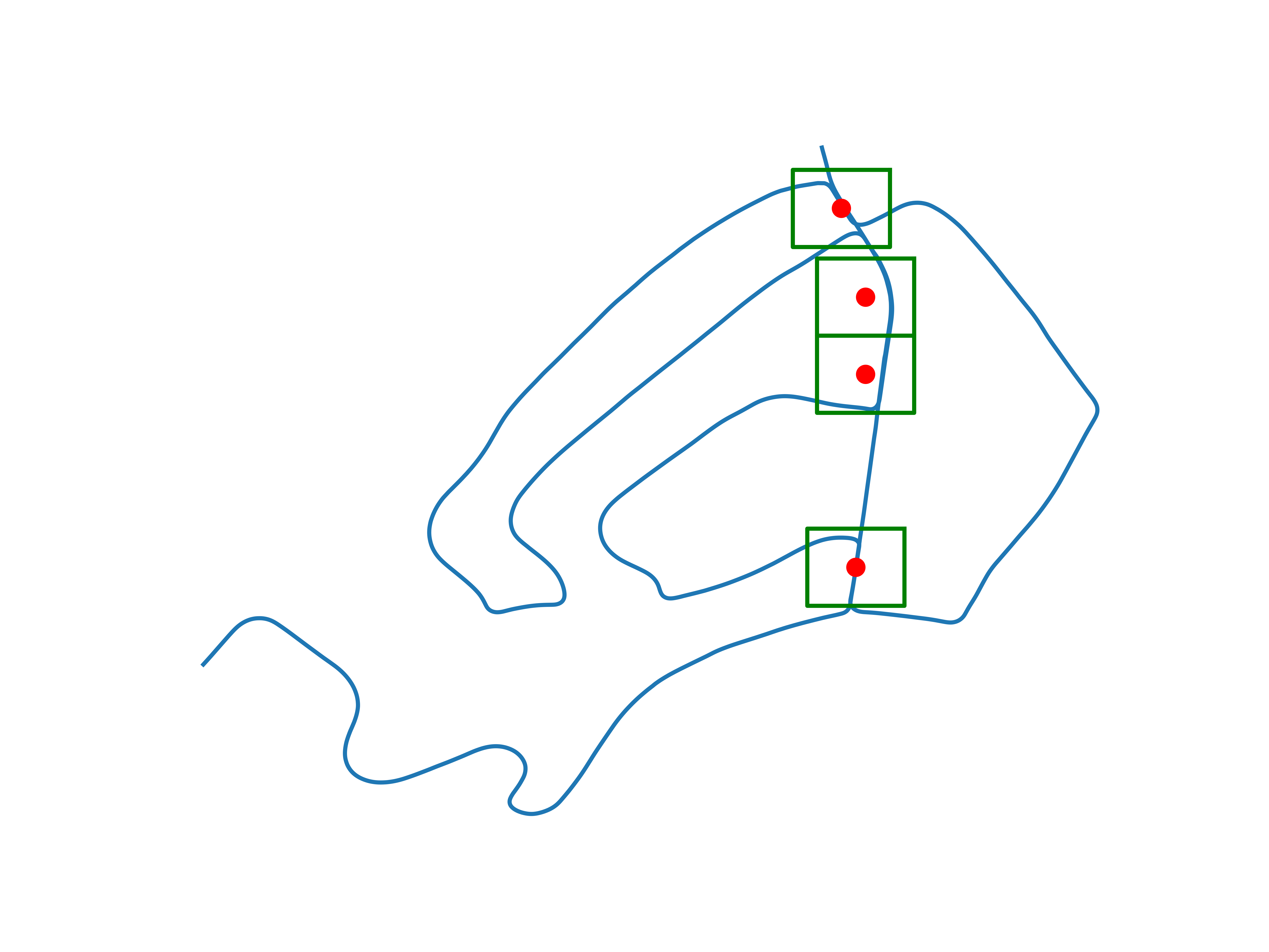
(b) Test regions in KITTI sequence 02.

Figure 8: We select non-overlapping regions from KITTI (sequences 00, 02). Samples from these regions are excluded from training. Note that these regions are selected because they were traversed for multiple times and are considered suitable for SLAM systems such as for loop closure detection or re-localization tasks.

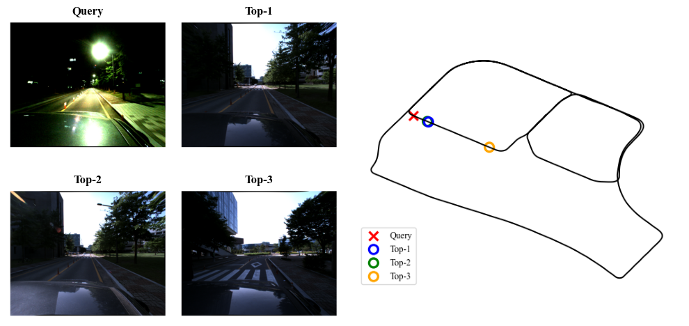
(a) ViViD++ campus night-day2 2D-2D failed.

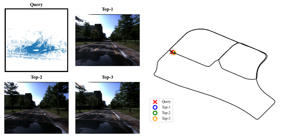
(b) ViViD++ campus night-day2 3D-2D succeeded.

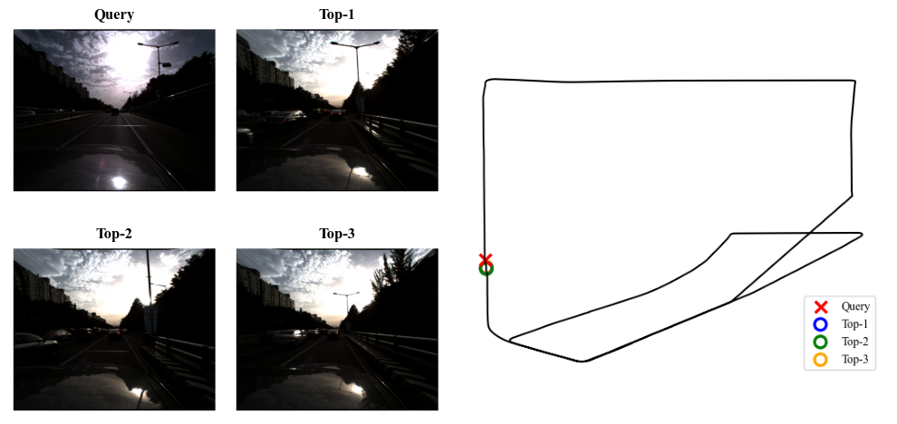
(c) ViViD++ city day1-day2 2D-2D failed.

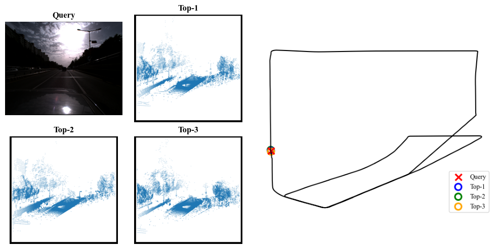
(d) ViViD++ city day1-day2 2D-3D succeeded.

Figure 9: Example of successful cross-modal retrievals (right) while the uni-modal retrievals fail (left) on the ViViD++ dataset. For each retrieval, the query and its top 3 retrievals are shown. Note that Fig. 9(a) and Fig. 9(b) are the example we’ve shown in Fig. 1 (main). Best viewed on a screen.

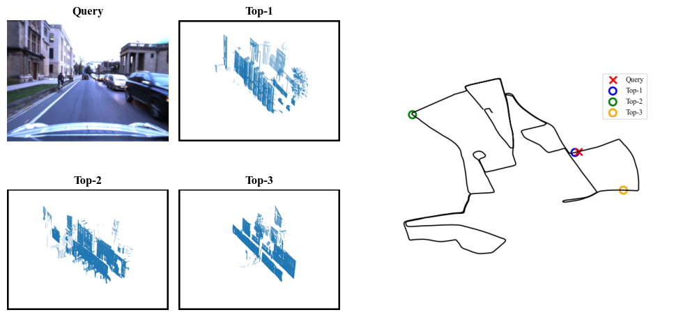
(a) 2D-3D retrieval

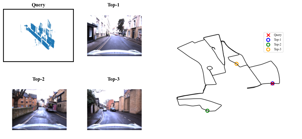
(b) 3D-2D retrieval

Figure 10: Example of successful retrieval results of VXP on the Oxford RobotCar dataset. For each retrieval, the query and its top 3 retrievals are shown. Best viewed on a screen.

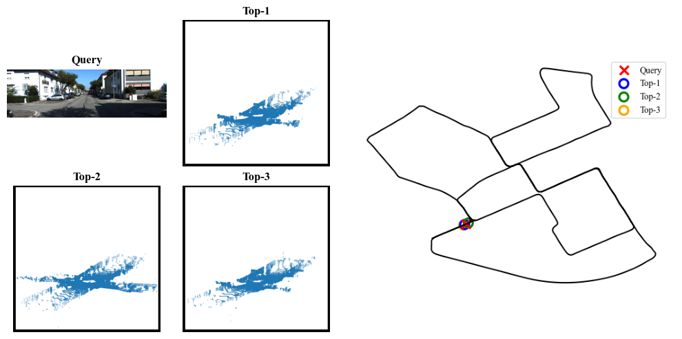
(a) KITTI (00) 2D-3D

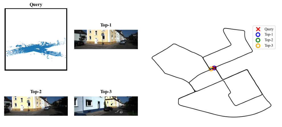
(b) KITTI (00) 3D-2D

Figure 11: Example of successful retrieval results of VXP on the KITTI Odometry Dataset. For each retrieval, the query and its top 3 retrievals are shown. Best viewed on a screen.

0.A.3 Qualitative Results

Given that cameras are sensitive to changes in illumination conditions, robust place recognition at night using images poses significant challenges as presented in Fig. 1 (main). In Fig. 9(c) we can observe the top 3 retrievals for 2D-2D retrieval being quite close to the query location. Nonetheless, they fall just slightly outside the accepted distance of 20 meters. This suggests that image-based place recognition struggles to precisely retrieve the geographically closest one when the images have challenging illuminations. However, VXP is successful in retrieving the closest candidates using 2D-3D cross-modal retrieval as illustrated in Fig. 9(d). This capability could explain why VXP exhibits slightly better top-1 2D-3D recall performance compared to its 2D-2D counterpart in Tab. 2 (main). Notably, VXP stands out as the only model (compared to [9, 19]) demonstrating such cross-modal retrieval capability across 2D-2D and 2D-3D scenarios. These observations underscore the versatility and effectiveness of cross-modal retrieval approaches in challenging real-world scenarios.

We demonstrate additional qualitative results of the cross-modal retrieval task on Oxford RobotCar Fig. 10 and KITTI Fig. 11 datasets.

0.A.4 Failure Cases

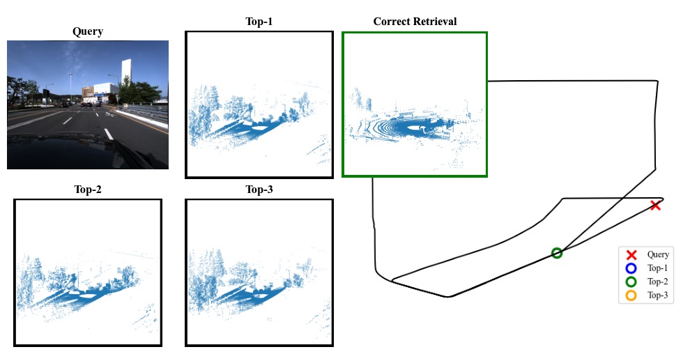
(a) ViViD++ City day1-day2 2D-3D failed.

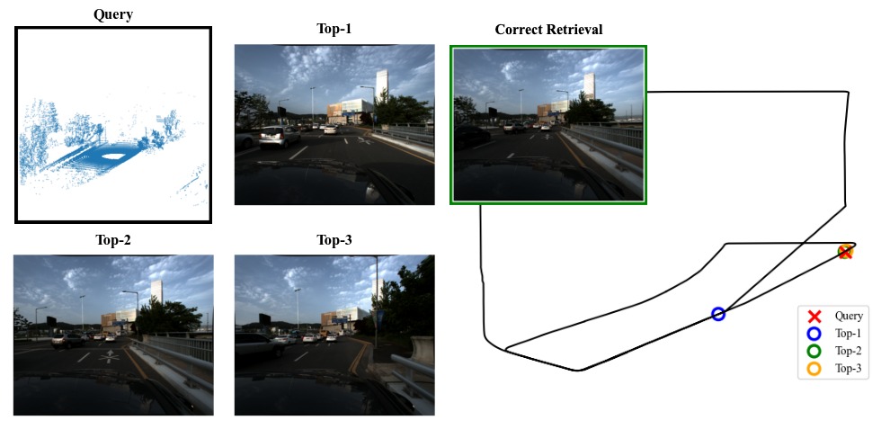
(b) ViViD++ City day1-day2 3D-2D failed.

Figure 12: Example of failed cross-modal retrievals due to repetitive scenes. Best viewed on a screen. For each retrieval, the query and its top 3 retrievals are shown. Note that we consider top-1 failure cases.

We identify some primary causes for failure in our estimations. Firstly, we note that repetitive structures such as highway roads cause confusion in our method and lead to incorrect retrievals. Notably, uni-modal methods also fail in such cases as shown in Fig. 12. Secondly, places where the environment contain a lot of empty space and few, far-away structures, resulting in meaningless sparse point clouds. One possible reason for a decreased performance lies in the projective nature of supervisory signal for our VXP. It is infeasible to learn a meaningful shared latent space and successfully perform cross-modal retrieval without establishing correspondences between voxels and pixels. Lastly, illumination conditions play a crucial part in retrieving the correct candidates using images as queries. Therefore, image feature map generated from poorly illuminated scene would obtain a bad-quality feature map (as shown in Fig. 1 of the main paper). Consequently, leveraging such images for successful cross-modal retrievals becomes considerably challenging as shown in Fig. 14.

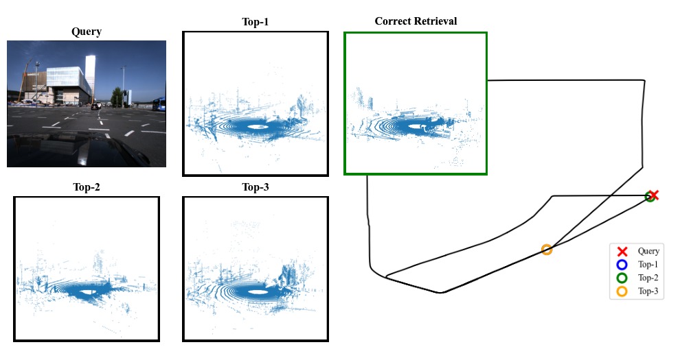
(a) ViViD++ City day1-day2 2D-3D failed.

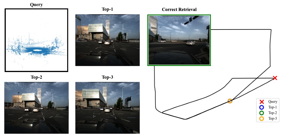
(b) ViViD++ City day1-day2 3D-2D failed.

Figure 13: Examples of incorrect cross-modal retrieval due to sparse meaningful structure in point cloud. For each retrieval, the query and its top 3 retrievals are shown. Note that we consider failure cases identified as top-1 candidate. Best viewed on a screen.

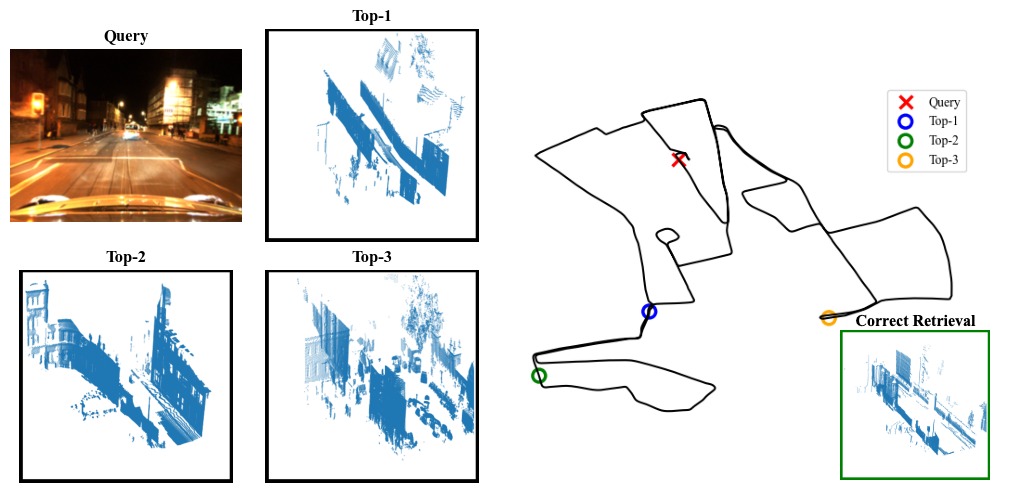
(a) Oxford RobotCar night-overcast 2D-3D failed.

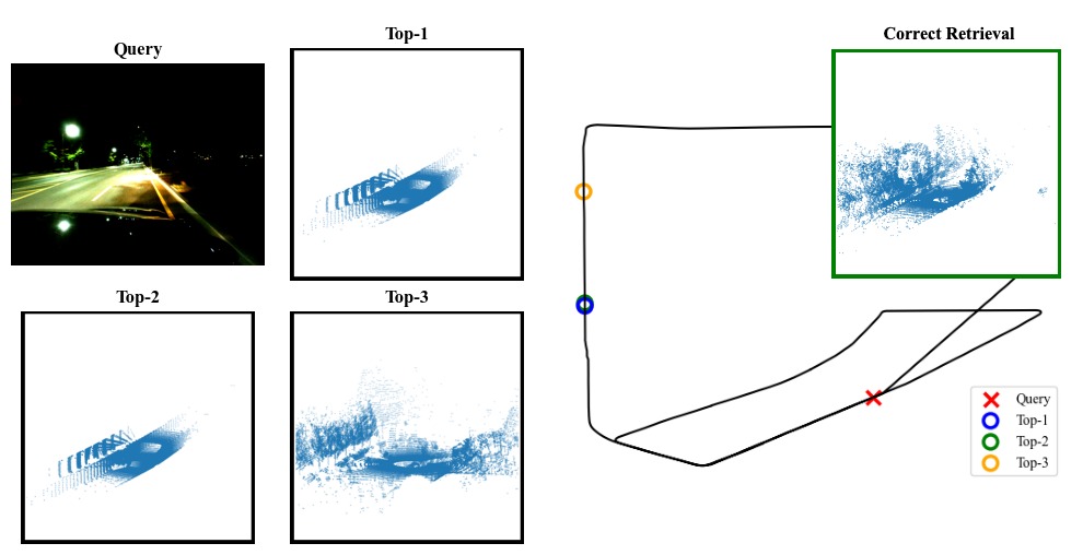
(b) ViViD++ City night-day2 2D-3D failed.

Figure 14: Examples of incorrect cross-modal retrieval due to bad lighting condition. For each retrieval, the query and its top 3 retrievals are shown. Note that we consider failure cases identified as top-1 candidate. Best viewed on a screen.

0.A.5 Correspondences in Local Feature Space

We visualize the local descriptors matching from different modalities as illustrated in Fig. 15. Note that the point cloud and image are not perfectly aligned and contain partially overlapping data since LiDAR and a camera are not synchronized. For example, here the distance between the image and the point cloud measures about 7 meters according to calibration + INS poses. In Fig. 15, the correspondences stemming from tree features can be accurately established. However, in regions where projected voxel features fall onto the ground region, we encounter challenges due to the plain and monotonous nature of respective image features. Therefore, capturing correspondences within the ground regions appears to be a difficult task. Nevertheless, it is worth noting that structures like buildings or other static distinct objects within the scene hold greater significance in the place recognition task. Since ground is constantly present in driving sequences, this misalignment only has minimal impact on distinctiveness of the estimated global descriptors and instead leverages correctly aligned correspondences to achieve state-of-the-art cross-modal performance.

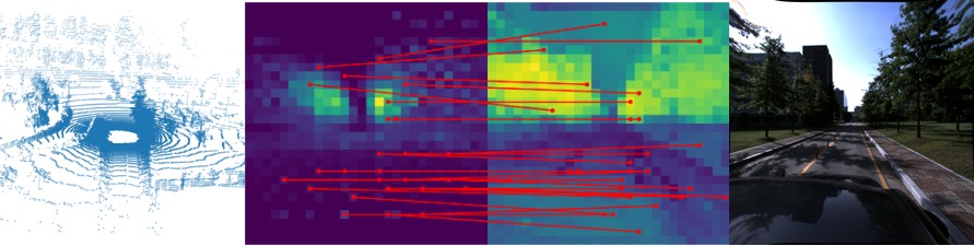
Figure 15: From left to right: original LiDAR point cloud, projected voxel feature map, image feature map, original RGB image closest to the LiDAR scan. In red we visualize local feature correspondences between the projected voxel feature map and the image feature map. LiDAR-image pair is taken from ViViD++ dataset.

References

- [1] Ali-bey, A., Chaib-draa, B., Giguère, P.: Gsv-cities: Toward appropriate supervised visual place recognition. Neurocomputing 513, 194–203 (2022)
- [2] Ali-Bey, A., Chaib-Draa, B., Giguere, P.: Mixvpr: Feature mixing for visual place recognition. In: Proceedings of the IEEE/CVF Winter Conference on Applications of Computer Vision. pp. 2998–3007 (2023)
- [3] Amir, S., Gandelsman, Y., Bagon, S., Dekel, T.: Deep vit features as dense visual descriptors. arXiv preprint arXiv:2112.05814 2(3), 4 (2021)
- [4] Arandjelovic, R., Gronat, P., Torii, A., Pajdla, T., Sivic, J.: Netvlad: Cnn architecture for weakly supervised place recognition. In: Proceedings of the IEEE conference on computer vision and pattern recognition. pp. 5297–5307 (2016)
- [5] Barnes, D., Gadd, M., Murcutt, P., Newman, P., Posner, I.: The oxford radar robotcar dataset: A radar extension to the oxford robotcar dataset. arXiv preprint arXiv: 1909.01300 (2019), https://arxiv.org/pdf/1909.01300
- [6] Berton, G., Masone, C., Caputo, B.: Rethinking visual geo-localization for large-scale applications. In: Proceedings of the IEEE/CVF Conference on Computer Vision and Pattern Recognition. pp. 4878–4888 (2022)
- [7] Caron, M., Touvron, H., Misra, I., Jégou, H., Mairal, J., Bojanowski, P., Joulin, A.: Emerging properties in self-supervised vision transformers. In: Proceedings of the IEEE/CVF international conference on computer vision. pp. 9650–9660 (2021)
- [8] Cattaneo, D., Vaghi, M., Ballardini, A.L., Fontana, S., Sorrenti, D.G., Burgard, W.: Cmrnet: Camera to lidar-map registration. In: 2019 IEEE intelligent transportation systems conference (ITSC). pp. 1283–1289. IEEE (2019)
- [9] Cattaneo, D., Vaghi, M., Fontana, S., Ballardini, A.L., Sorrenti, D.G.: Global visual localization in lidar-maps through shared 2d-3d embedding space. In: 2020 IEEE International Conference on Robotics and Automation (ICRA). pp. 4365–4371. IEEE (2020)
- [10] Cattaneo, D., Vaghi, M., Valada, A.: Lcdnet: Deep loop closure detection and point cloud registration for lidar slam. IEEE Transactions on Robotics 38(4), 2074–2093 (2022)
- [11] Fan, Z., Song, Z., Liu, H., Lu, Z., He, J., Du, X.: Svt-net: Super light-weight sparse voxel transformer for large scale place recognition. AAAI (2022)
- [12] Feng, M., Hu, S., Ang, M.H., Lee, G.H.: 2d3d-matchnet: Learning to match keypoints across 2d image and 3d point cloud. In: 2019 International Conference on Robotics and Automation (ICRA). pp. 4790–4796. IEEE (2019)
- [13] Gálvez-López, D., Tardos, J.D.: Bags of binary words for fast place recognition in image sequences. IEEE Transactions on Robotics 28(5), 1188–1197 (2012)
- [14] Geiger, A., Lenz, P., Urtasun, R.: Are we ready for autonomous driving? the kitti vision benchmark suite. In: 2012 IEEE conference on computer vision and pattern recognition. pp. 3354–3361. IEEE (2012)
- [15] He, K., Zhang, X., Ren, S., Sun, J.: Deep residual learning for image recognition. In: Proceedings of the IEEE conference on computer vision and pattern recognition. pp. 770–778 (2016)
- [16] Komorowski, J.: Minkloc3d: Point cloud based large-scale place recognition. In: Proceedings of the IEEE/CVF Winter Conference on Applications of Computer Vision. pp. 1790–1799 (2021)
- [17] Komorowski, J., Wysoczańska, M., Trzcinski, T.: Minkloc++: lidar and monocular image fusion for place recognition. In: 2021 International Joint Conference on Neural Networks (IJCNN). pp. 1–8. IEEE (2021)
- [18] Lee, A.J., Cho, Y., Shin, Y.s., Kim, A., Myung, H.: Vivid++: Vision for visibility dataset. IEEE Robotics and Automation Letters 7(3), 6282–6289 (2022)
- [19] Lee, A.J., Song, S., Lim, H., Lee, W., Myung, H.: Lc2: Lidar-camera loop constraints for cross-modal place recognition. IEEE Robotics and Automation Letters 8, 3589–3596 (2023), https://api.semanticscholar.org/CorpusID:258187613
- [20] Leyva-Vallina, M., Strisciuglio, N., Petkov, N.: Data-efficient large scale place recognition with graded similarity supervision. In: Proceedings of the IEEE/CVF Conference on Computer Vision and Pattern Recognition. pp. 23487–23496 (2023)
- [21] Li, J., Lee, G.H.: Deepi2p: Image-to-point cloud registration via deep classification. In: Proceedings of the IEEE/CVF Conference on Computer Vision and Pattern Recognition. pp. 15960–15969 (2021)
- [22] Liu, Z., Zhou, S., Suo, C., Yin, P., Chen, W., Wang, H., Li, H., Liu, Y.H.: Lpd-net: 3d point cloud learning for large-scale place recognition and environment analysis. In: Proceedings of the IEEE/CVF International Conference on Computer Vision. pp. 2831–2840 (2019)
- [23] Ma, J., Zhang, J., Xu, J., Ai, R., Gu, W., Chen, X.: Overlaptransformer: An efficient and yaw-angle-invariant transformer network for lidar-based place recognition. IEEE Robotics and Automation Letters 7(3), 6958–6965 (2022)
- [24] Maddern, W., Pascoe, G., Linegar, C., Newman, P.: 1 year, 1000 km: The oxford robotcar dataset. The International Journal of Robotics Research 36(1), 3–15 (2017)
- [25] Pan, Y., Xu, X., Li, W., Cui, Y., Wang, Y., Xiong, R.: Coral: Colored structural representation for bi-modal place recognition. In: 2021 IEEE/RSJ International Conference on Intelligent Robots and Systems (IROS). pp. 2084–2091. IEEE (2021)
- [26] Philbin, J., Chum, O., Isard, M., Sivic, J., Zisserman, A.: Object retrieval with large vocabularies and fast spatial matching. In: 2007 IEEE conference on computer vision and pattern recognition. pp. 1–8. IEEE (2007)
- [27] Qi, C.R., Su, H., Mo, K., Guibas, L.J.: Pointnet: Deep learning on point sets for 3d classification and segmentation. In: Proceedings of the IEEE conference on computer vision and pattern recognition. pp. 652–660 (2017)
- [28] Qi, C.R., Yi, L., Su, H., Guibas, L.J.: Pointnet++: Deep hierarchical feature learning on point sets in a metric space. Advances in neural information processing systems 30 (2017)
- [29] Radenović, F., Tolias, G., Chum, O.: Fine-tuning cnn image retrieval with no human annotation. IEEE transactions on pattern analysis and machine intelligence 41(7), 1655–1668 (2018)
- [30] Ren, S., Zeng, Y., Hou, J., Chen, X.: Corri2p: Deep image-to-point cloud registration via dense correspondence. IEEE Transactions on Circuits and Systems for Video Technology 33(3), 1198–1208 (2022)
- [31] Schroff, F., Kalenichenko, D., Philbin, J.: Facenet: A unified embedding for face recognition and clustering. In: Proceedings of the IEEE conference on computer vision and pattern recognition. pp. 815–823 (2015)
- [32] Simonyan, K., Zisserman, A.: Very deep convolutional networks for large-scale image recognition. arXiv preprint arXiv:1409.1556 (2014)
- [33] Uy, M.A., Lee, G.H.: Pointnetvlad: Deep point cloud based retrieval for large-scale place recognition. In: Proceedings of the IEEE conference on computer vision and pattern recognition. pp. 4470–4479 (2018)
- [34] Wang, G., Zheng, Y., Guo, Y., Liu, Z., Zhu, Y., Burgard, W., Wang, H.: End-to-end 2d-3d registration between image and lidar point cloud for vehicle localization. arXiv preprint arXiv:2306.11346 (2023)
- [35] Watson, J., Mac Aodha, O., Prisacariu, V., Brostow, G., Firman, M.: The temporal opportunist: Self-supervised multi-frame monocular depth. In: Proceedings of the IEEE/CVF Conference on Computer Vision and Pattern Recognition. pp. 1164–1174 (2021)
- [36] Xia, Y., Gladkova, M., Wang, R., Li, Q., Stilla, U., Henriques, J.a.F., Cremers, D.: Casspr: Cross attention single scan place recognition. In: Proceedings of the IEEE/CVF International Conference on Computer Vision (ICCV). pp. 8461–8472 (October 2023)
- [37] Xia, Y., Shi, L., Ding, Z., Henriques, J.F., Cremers, D.: Text2loc: 3d point cloud localization from natural language. In: Proceedings of the IEEE/CVF Conference on Computer Vision and Pattern Recognition (2024)
- [38] Xia, Y., Xu, Y., Li, S., Wang, R., Du, J., Cremers, D., Stilla, U.: Soe-net: A self-attention and orientation encoding network for point cloud based place recognition. In: Proceedings of the IEEE/CVF Conference on computer vision and pattern recognition. pp. 11348–11357 (2021)
- [39] Yan, Y., Mao, Y., Li, B.: Second: Sparsely embedded convolutional detection. Sensors 18(10), 3337 (2018)
- [40] Zhou, Y., Tuzel, O.: Voxelnet: End-to-end learning for point cloud based 3d object detection. In: Proceedings of the IEEE conference on computer vision and pattern recognition. pp. 4490–4499 (2018)
- [41] Zhou, Z., Zhao, C., Adolfsson, D., Su, S., Gao, Y., Duckett, T., Sun, L.: Ndt-transformer: Large-scale 3d point cloud localisation using the normal distribution transform representation. In: 2021 IEEE International Conference on Robotics and Automation (ICRA). pp. 5654–5660. IEEE (2021)