Co-Optimization of Environment and Policies for Decentralized Multi-Agent Navigation

Abstract

This work views the multi-agent system and its surrounding environment as a co-evolving system, where the behavior of one affects the other. The goal is to take both agent actions and environment configurations as decision variables, and optimize these two components in a coordinated manner to improve some measure of interest. Towards this end, we consider the problem of decentralized multi-agent navigation in cluttered environments. By introducing two sub-objectives of multi-agent navigation and environment optimization, we propose an agent-environment co-optimization problem and develop a coordinated algorithm that alternates between these sub-objectives to search for an optimal synthesis of agent actions and obstacle configurations in the environment; ultimately, improving the navigation performance. Due to the challenge of explicitly modeling the relation between agents, environment and performance, we leverage policy gradient to formulate a model-free learning mechanism within the coordinated framework. A formal convergence analysis shows that our coordinated algorithm tracks the local minimum trajectory of an associated time-varying non-convex optimization problem. Extensive numerical results corroborate theoretical findings and show the benefits of co-optimization over baselines. Interestingly, the results also indicate that optimized environment configurations are able to offer structural guidance that is key to de-conflicting agents in motion.

I Introduction

Multi-agent systems comprise multiple decision-making agents that interact in a shared environment to achieve common or individual goals. They present an attractive solution to spatially distributed tasks, wherein efficient and safe motion planning among moving agents and obstacles is one of the central problems [1, 2, 3, 4, 5, 6, 7, 8]. The behavior of multi-agent systems, both living and artificial, is influenced by the structure of their surrounding environment, where spatial constraints may result in dead-locks, live-locks and prioritization conflicts even for state-of-the-art algorithms [9, 10], highlighting the impact of the environment on agents’ performance. Yet, despite the entanglement of these two components, coordinated optimization of multi-agent policies and environment configurations has received little attention thus far.

With advances in programmable and responsive buildings, reconfigurable and automated environments are emerging as a new trend [11, 12, 13, 14]. In parallel to developing agent policies, this enabling technology allows to re-configure the spatial layout of the environment as a means to improve some objective performance measure of the multi-agent system. The latter is especially appealing when agents are expected to solve repetitive tasks in structured settings (like warehouses, factories, restaurants, etc.). While it is possible to hand-design environment configurations, such a procedure is inefficient and sub-optimal [15].

Recent works have suggested that significant benefits can be reaped by either adapting the environment to agent policies or tuning agent policies based on the environment [16, 17, 18, 19, 20, 21]. These insights motivate the coupling of the environment configuration design with the agents’ policy development. In this context, the goal of this work is to consider the obstacle layout of the environment as a decision variable, as well as the navigation policy of agents, and propose a system-level co-optimization problem that simultaneously optimizes these two components; ultimately, establishing a symbiotic agent-environment co-evolving system that maximizes the navigation performance of the multi-agent system. Applications of agent-environment co-optimization include warehouse logistics (e.g., finding the optimal shelf positions and robot policies for cargo transportation [22]), search and rescue (e.g., generating the best passages and rescue strategies for trapped victims [23]), city planning (e.g., designing the optimal one-way routes and autonomous vehicles for traffic efficiency [24]), and digital entertainment (e.g., building the best gaming scene and non-player character behaviors for video games [25]).

Figure 1: Agent-environment coordinated optimization is an optimization process that alternates between a multi-agent navigation policy (parameterized with $\theta_{a}$) and an environment generative model (parameterized with $\theta_{o}$), searching for an optimal pair of these two components that maximizes the overall system performance (e.g., a user-defined objective function). In the above example, it optimizes the navigation policy with reinforcement learning (e.g., blue trajectories become yellow trajectories) and the environment configuration with unsupervised learning (e.g., grey obstacles become green obstacles), in an alternating manner.

In pursuit of this goal, we propose a coordinated optimization algorithm that alternates between the synthesis of navigation behavior and environment design. Due to the challenge of explicitly modeling the relation between agents, environment and navigation performance, we pose the problem in a model-free learning framework and introduce two sub-objectives for multi-agent navigation and environment optimization, respectively. We parameterize the navigation policy of agents with a graph neural network (GNN) for decentralized implementation and use a generative model of the environment, parameterized by a deep neural network (DNN). The two models are updated with respect to two sub-objectives in an alternating manner, pursuing an optimal pair of navigation and generative parameters that maximizes the multi-agent system performance – see Fig. 1 for an overview of the agent-environment coordinated optimization framework. More in details, our contributions are as follows:

• We define the problem of agent-environment co-optimization, which searches for an optimal pair of environment configuration and multi-agent policy to jointly maximize the navigation performance.

• We develop a coordinated method that optimizes the navigation policy of the agents with reinforcement learning and a generative model of the environment configuration with unsupervised learning, based on two sub-objectives, in an alternating manner. We formulate a model-free learning mechanism within the coordinated framework, which overcomes the challenge of modeling the explicit relation between agents, environment and performance.

• We provide a formal convergence analysis for the proposed coordinated method by detailing its relation with an associated time-varying non-convex optimization problem and an ordinary differential equation.

• We perform experiments to evaluate the proposed method. The results corroborate theoretical findings and provide novel insights regarding the relationship between the environment and the multi-agent system. I.e., we show how appropriately designed environments are able to guide multi-agent navigation through targeted spatial deconfliction.

Related work. The idea of co-optimization (or co-design) in robotics can be traced back to work on embodied cognitive science [26], which emphasizes the importance of the robot body and its interaction with the environment for achieving robust behavior. Motivated by this idea, research in the domain of robot co-design aims to find optimized controller, sensing and morphology, such that they together produce the desired performance [27, 28, 29]. A few seminal works tackled this problem with an evolutionary approach that co-optimizes objectives [30, 31]. More recently, Schaff et al. [32] employed reinforcement learning to learn both the policy and morphology design parameters in an alternating manner, where a single shared policy controls the distribution of different robot designs. Within the multi-agent domain, the concept of co-optimization has mainly been leveraged to allocate physical resources to agent tasks. The work in [33] proposed a joint equilibrium policy search method that encourages agents to cooperate to reach states maximizing a global reward, while Zhang et al. [34] developed a multi-level search approach that co-optimizes agent placements with task assignment and scheduling. In a similar vein, Jain et al. [35] used online multi-agent reinforcement learning to co-optimize cores, caches and on-chip networks. The works in [36, 37] considered the problem of co-optimizing mobility and communication among agents, and designed schedule policies that minimize the total energy. While broadly similar in their ideas, none of the aforementioned works consider co-optimizing the environment and navigation behaviors to improve the system performance of multiple agents (i.e., robots).

The key challenge of co-optimization stands in the fact that the explicit relation between agents, environment and system performance is generally not known (and hard to model), compounding the difficulty of solving the joint problem. The agent-environment relationship has been previously explored. The works in [38, 39] identified the existence of congestion and deadlocks in undesirable environments and developed trajectory planning methods for agents to escape from these potential deadlocks, while [18] introduced the concept of “well-formed” environment where the navigation tasks of all agents can be carried out successfully without collision. Wu et al. [7] showed that the environment shape can result in distinct path prospects for different agents and proposed to leverage this information for coordinating agents’ motion. Additionally, [40] focused on adversarial environments and developed resilient navigation algorithms for agents in these environments. However, none of these works consider both the environment as well as the agents’ policies as decision variables in a system-level optimization problem (with the aim of improving navigation performance).

More similar in vein to our work, Hauser [41, 42] attempted to remove obstacles from the environment to improve the agent’s navigation performance, while focusing on a single agent scenario. The work in [13] extended a related idea to the multi-agent setting, to search over all possible environment configurations to find the best solution for agents. However, the technique is limited to discrete settings, and only considers obstacle removal (in contrast to general re-configuration). The problem of multi-agent pick-up and delivery also explores the relationship between agents and environment [43, 44, 45]. However, it considers environment changes as pre-defined tasks and assigns agents to complete these tasks – constituting a different problem that is defined only in a discrete setting.

II Problem Formulation

Let ${\mathcal{E}}$ be a $2$-D environment with $m$ obstacles ${\mathcal{O}}=\{O_{1},\ldots,O_{m}\}$. The obstacles can be of any shape, and are located randomly in an obstacle region $\Delta$. Consider a multi-agent system with $n$ agents ${\mathcal{A}}=\{A_{i}\}_{i=1}^{n}$ distributed in ${\mathcal{E}}$. The agents are initialized randomly in the starting region ${\mathcal{S}}$ and deploy a navigation policy $\pi_{a}$ to move towards the destination region ${\mathcal{D}}$. We are interested in decentralized multi-agent navigation problems, where agents have access to their own states, e.g., positions and velocities, and exchange local observations with neighboring agents in the communication range. Our performance metrics include traveled distance, average speed and collision avoidance, which depend not only on the agents’ policy $\pi_{a}$ but also the surrounding environment ${\mathcal{E}}$. For example, we may facilitate the navigation by either developing an efficient policy, or designing a “well-formed” environment with an appropriate obstacle layout, or both.

This insight motivates a view of agents ${\mathcal{A}}$ and their environment ${\mathcal{E}}$ as a co-evolving system. The problem of agent-environment co-optimization then considers both components as decision variables. In particular, there are two objectives of concern: (i) finding the optimal policy $\pi^{*}_{a}$ for agents to reach goal positions without colliding with one another nor with obstacles; (ii) finding the optimal obstacle layout for the environment ${\mathcal{E}}^{*}$. The goal is to achieve these objectives simultaneously, i.e., improving the navigation policy while, towards the same end, optimizing the obstacle layout. This allows to explore the coupling between the agents’ policy and the environment configuration, to find an optimal pair $(\pi_{a}^{*},{\mathcal{E}}^{*})$ that maximizes the performance. In the following subsections, we first introduce individual problem components and then formulate the agent-environment co-optimization problem.

II-A Multi-Agent Navigation

We consider the agents ${\mathcal{A}}$ initialized at starting positions ${\mathbf{S}}=[{\mathbf{s}}_{1},\ldots,{\mathbf{s}}_{n}]\in{\mathcal{S}}$ and tasked to navigate towards goal positions ${\mathbf{D}}=[{\mathbf{d}}_{1},\ldots,{\mathbf{d}}_{n}]\in{\mathcal{D}}$. Let ${\mathbf{X}}_{a}=[{\mathbf{x}}_{a1},\ldots,{\mathbf{x}}_{an}]$ be the agent states and ${\mathbf{U}}_{a}=[{\mathbf{u}}_{a1},\ldots,{\mathbf{u}}_{am}]$ the agent actions. For example, ${\mathbf{X}}_{a}$ are the positions or velocities and ${\mathbf{U}}_{a}$ are the accelerations. Let $\pi_{a}({\mathbf{U}}_{a}|{\mathbf{X}}_{a})$ be the navigation policy that controls the agents moving from ${\mathbf{S}}$ to ${\mathbf{D}}$, which is a distribution of the agent actions ${\mathbf{U}}_{a}$ conditioned on the agent states ${\mathbf{X}}_{a}$. We model the navigation process as a sequential decision-making problem, where agents take actions based on instantaneous states across time steps $t$.

The navigation performance of the multi-agent system is determined by the navigation task, the moving capacity of the agents (e.g., their maximal velocity) and the physical restrictions of the environment (e.g., obstacle blocking). In this context, we use an objective function $f({\mathbf{S}},{\mathbf{D}},\pi_{a},{\mathcal{E}})$ that depends on the initial positions ${\mathbf{S}}$, the goal positions ${\mathbf{D}}$, the navigation policy $\pi_{a}$, and the environment ${\mathcal{E}}$. The goal of multi-agent navigation is to find the optimal $\pi_{a}^{*}$ that maximizes $f({\mathbf{S}},{\mathbf{D}},\pi_{a}^{*},{\mathcal{E}})$ given the navigation task $({\mathbf{S}},{\mathbf{D}})$ and the environment ${\mathcal{E}}$.

II-B Environment Optimization

The obstacle layout ${\mathcal{O}}$, e.g., the obstacle position and the obstacle size, determines the environment configuration ${\mathcal{E}}$ for multi-agent navigation. Let $\pi_{o}({\mathcal{O}}|{\mathbf{S}},{\mathbf{D}})$ be the generative model that configures the obstacles in the work space, which is a distribution of the obstacle layout ${\mathcal{O}}$ conditioned on the navigation task, i.e., the initial and goal positions $({\mathbf{S}},{\mathbf{D}})$ of the agents ${\mathcal{A}}$.

Since the environment ${\mathcal{E}}$ is determined by the obstacle layout and the latter is determined by the generative model $\pi_{o}$, we can re-write the objective function of the multi-agent navigation as $f({\mathbf{S}},{\mathbf{D}},\pi_{a},\pi_{o})$. The goal of environment optimization is to find the optimal $\pi^{*}_{o}$ that generates the environment ${\mathcal{E}}^{*}$ to maximize $f({\mathbf{S}},{\mathbf{D}},\pi_{a},\pi_{o}^{*})$ given the navigation task $({\mathbf{S}},{\mathbf{D}})$ and the navigation policy $\pi_{a}$.

II-C Agent-Environment Co-Optimization

We use definitions from the individual sub-problems (Sections II-A and II-B) to formulate the problem of agent-environment co-optimization, which searches for an optimal pair of the navigation policy and the generative model $(\pi_{a}^{*},\pi_{o}^{*})$ that maximizes the navigation performance of the multi-agent system, i.e., the objective function $f({\mathbf{S}},{\mathbf{D}},\pi_{a},\pi_{o})$, in a joint manner. Specifically, we define the agent-environment co-optimization problem as

$$\operatornamewithlimits{argmax}_{\pi_{a},\pi_{o}}\leavevmode\nobreak\ f({\mathbf{S}},{\mathbf{D}},\pi_{a},\pi_{o})$$ (1)

$$\leavevmode\nobreak\ \leavevmode\nobreak\ \leavevmode\nobreak\ \leavevmode\nobreak\ \text{s.t.}\leavevmode\nobreak\ \leavevmode\nobreak\ \leavevmode\nobreak\ \pi_{a}({\mathbf{U}}_{a}|{\mathbf{X}}_{a})\in{\mathcal{U}}_{a},\leavevmode\nobreak\ \pi_{o}({\mathcal{O}}|{\mathbf{S}},{\mathbf{D}})\in{\mathcal{P}}_{o},$$

where ${\mathcal{U}}_{a}$ is the action space of the agents and ${\mathcal{P}}_{o}$ is the feasible set of the obstacle layout. The preceding problem is difficult due to the following challenges:

1. The objective function $f({\mathbf{S}},{\mathbf{D}},\pi_{a},\pi_{o})$ depends on the multi-agent system and the environment. It is, however, impractical to model this relationship analytically, hence, precluding the application of conventional model-based methods. For the same reason, heuristic methods will perform poorly.

2. The navigation policy $\pi_{a}({\mathbf{U}}_{a}|{\mathbf{X}}_{a})$ generates sequential agent actions based on instantaneous states across time steps, while the generative model $\pi_{o}({\mathcal{O}}|{\mathbf{S}},{\mathbf{D}})$ generates a one-shot (time-invariant) environment configuration based on the navigation task before agents start to move. The navigation policy needs unrolling to be evaluated for any generated environment. Hence, $\pi_{a}$ and $\pi_{o}$ have different inner-working mechanisms and cannot be optimized in the same way, which complicates the joint optimization.

3. The navigation policy $\pi_{a}({\mathbf{U}}_{a}|{\mathbf{X}}_{a})$ and the generative model $\pi_{o}({\mathcal{O}}|{\mathbf{S}},{\mathbf{D}})$ are arbitrary mappings from ${\mathbf{X}}_{a}$ and $({\mathbf{S}},{\mathbf{D}})$ to ${\mathbf{U}}_{a}$ and ${\mathcal{O}}$, which can take any function forms and thus are infinitely dimensional.

4. The action space of the agents ${\mathcal{U}}_{a}$ can be either discrete or continuous and the feasible set ${\mathcal{P}}_{o}$ can be either convex or non-convex. This leads to complex constraints on the feasible solution.

Due to the above challenges, we propose to solve problem (1) with a model-free learning-based approach, in which we alternate between two optimization sub-objectives. Specifically, we parameterize the navigation policy $\pi_{a}({\mathbf{U}}_{a}|{\mathbf{X}}_{a})$ by a graph neural network with parameters $\boldsymbol{\theta}_{a}$, and the generative model $\pi_{o}({\mathcal{O}}|{\mathbf{S}},{\mathbf{D}})$ by a deep neural network with parameters $\boldsymbol{\theta}_{o}$. We update the navigation parameters $\boldsymbol{\theta}_{a}$ with actor-critic reinforcement learning (RL), and the generative parameters $\boldsymbol{\theta}_{o}$ with a policy gradient ascent (unsupervised learning), in an alternating manner, to find an optimal pair $(\boldsymbol{\theta}_{a}^{*},\boldsymbol{\theta}_{o}^{*})$ that maximizes the navigation performance. The proposed approach overcomes challenge (i) with its model-free implementation, challenge (ii) with its alternating optimization, challenge (iii) with its finite parameterization, and challenge (iv) with its appropriate selection of policy / generative distributions.

III Coordinated Optimization Methodology

We begin by re-formulating problem 1 as an optimization problem with two sub-objectives:

$$\operatornamewithlimits{argmax}_{\pi_{a}}\leavevmode\nobreak\ f({\mathbf{S}},{\mathbf{D}},\pi_{a},{\mathcal{E}})\leavevmode\nobreak\ \text{s.t.}\leavevmode\nobreak\ \pi_{a}({\mathbf{U}}_{a}|{\mathbf{X}}_{a})\in{\mathcal{U}}_{a},$$ (2)

$$\operatornamewithlimits{argmax}_{\pi_{o}}\leavevmode\nobreak\ f({\mathbf{S}},{\mathbf{D}},\pi_{a},\pi_{o})\leavevmode\nobreak\ \text{s.t.}\leavevmode\nobreak\ \pi_{o}({\mathcal{O}}|{\mathbf{S}},{\mathbf{D}})\in{\mathcal{U}}_{o}.$$ (3)

Sub-objective (2) optimizes the navigation policy given the environment ${\mathcal{E}}$, while sub-objective (3) optimizes the generative model given the navigation policy of the agents $\pi_{a}$.

III-A Navigation Policy

We are interested in synthesizing a decentralized navigation policy $\pi_{a}$ that generates sequential agent actions as a function of local observations. To do so, we define a Markov decision process wherein, at time $t$, agents observe states ${\mathbf{X}}_{a}^{(t)}=[{\mathbf{x}}_{a1}^{(t)},\ldots,{\mathbf{x}}_{an}^{(t)}]$ and take actions ${\mathbf{U}}_{a}^{(t)}=[{\mathbf{u}}_{a1}^{(t)},\ldots,{\mathbf{u}}_{an}^{(t)}]$. In the decentralized setting, each agent $A_{i}$ only has access to its own state ${\mathbf{x}}_{ai}^{(t)}$ and can communicate with its neighboring agents to collect the neighborhood information ${\mathbf{X}}_{a{\mathcal{N}}_{i}}^{(t)}=\{{\mathbf{x}}_{aj}^{(t)}\}_{j\in{\mathcal{N}}_{i}}$, where ${\mathcal{N}}_{i}$ is the set of neighboring agents within communication range. The navigation policy $\pi_{a}$ generates the agent action ${\mathbf{u}}_{ai}^{(t)}$ based on the local states $\{{\mathbf{x}}_{ai}^{(t)},{\mathbf{X}}_{a{\mathcal{N}}_{i}}^{(t)}\}$ for $i=1,\ldots,n$, and these actions ${\mathbf{U}}_{a}^{(t)}$ create transitions from ${\mathbf{X}}_{a}^{(t)}$ to ${\mathbf{X}}_{a}^{(t+1)}$ based on the transition probability function $P_{a}({\mathbf{X}}_{a}^{(t+1)}|{\mathbf{X}}_{a}^{(t)},{\mathbf{U}}_{a}^{(t)},{\mathcal{E}})$, which is a distribution of states conditioned on the previous states, actions and environment. Let $r_{ai}({\mathbf{X}}_{a}^{(t)},{\mathbf{U}}_{a}^{(t)},{\mathcal{E}})$ be the reward function of agent $A_{i}$ for $i=1,...,n$, which represents the instantaneous navigation performance at time $t$. The reward function of the multi-agent system is the navigation performance averaged over $n$ agents

$$r_{a}^{(t)}=\frac{1}{n}\sum_{i=1}^{n}r_{ai}({\mathbf{X}}_{a}^{(t)},{\mathbf{U}}_{a}^{(t)},{\mathcal{E}}).$$ (4)

With the discount factor $\gamma$ that accounts for the future rewards, the expected discounted reward is given by

$$R_{a}({\mathbf{S}},{\mathbf{D}},\pi_{a},{\mathcal{E}}) =\mathbb{E}\Big{[}\sum_{t=0}^{\infty}\gamma^{t}r_{a}^{(t)}\Big{]}$$ (5)

$$=\mathbb{E}\Big{[}\sum_{t=0}^{\infty}\frac{\gamma^{t}}{n}\sum_{i=1}^{n}r_{ai}({\mathbf{X}}_{a}^{(t)},{\mathbf{U}}_{a}^{(t)},{\mathcal{E}})\Big{]},$$

where the initial states ${\mathbf{X}}_{a}^{(0)}$ are determined by the initial and goal positions $({\mathbf{S}},{\mathbf{D}})$, and $\mathbb{E}[\cdot]$ is w.r.t. the navigation policy $\pi_{a}$ and the state transition probability $P_{a}$. By parameterizing $\pi_{a}$ with an information processing architecture $\boldsymbol{\Phi}_{a}({\mathbf{X}}_{a},\boldsymbol{\theta}_{a})$ of parameters $\boldsymbol{\theta}_{a}$ (e.g., graph neural network – see Appendix B), we can represent the expected discounted reward as $R_{a}({\mathbf{S}},{\mathbf{D}},\boldsymbol{\theta}_{a},{\mathcal{E}})$ and the goal is to find the optimal parameters $\boldsymbol{\theta}^{*}_{a}$ that maximize $R_{a}({\mathbf{S}},{\mathbf{D}},\boldsymbol{\theta}_{a},{\mathcal{E}})$. The expected discounted reward in (5) is equivalent to the sub-objective in (2) and thus, we can re-formulate the problem in the RL domain as

$$\operatornamewithlimits{argmax}_{\boldsymbol{\theta}_{a}}\leavevmode\nobreak\ R_{a}({\mathbf{S}},{\mathbf{D}},\boldsymbol{\theta}_{a},{\mathcal{E}})\leavevmode\nobreak\ \text{s.t.}\leavevmode\nobreak\ \boldsymbol{\Phi}_{a}({\mathbf{X}}_{a},\boldsymbol{\theta}_{a})\in{\mathcal{U}}_{a}.$$ (6)

III-B Generative Model

We use a generative model to learn the process of environment design. Different from the navigation policy $\pi_{a}$ that synthesizes sequential time-varying agent actions, the generative model $\pi_{o}$ generates a static environment (i.e., obstacle layout) in one shot before agents start to move. This allows us to re-formulate the sub-objective in (3) as a stochastic optimization problem. To do so, we assume the initial positions ${\mathbf{S}}$, goal positions ${\mathbf{D}}$ and parameterized navigation policy $\boldsymbol{\Phi}_{a}({\mathbf{X}}_{a},\boldsymbol{\theta}_{a})$ are given, and hence, can measure the navigation performance with the expected discounted reward $R_{a}({\mathbf{S}},{\mathbf{D}},\boldsymbol{\theta}_{a},{\mathcal{E}})$ [cf. (6)]. By parameterizing the generative model $\pi_{o}$ with an information processing architecture $\boldsymbol{\Phi}_{o}({\mathbf{S}},{\mathbf{D}},\boldsymbol{\theta}_{o})$ of parameters $\boldsymbol{\theta}_{o}$ (e.g., deep neural network – see Appendix B), we can represent the expected discounted reward as $R_{a}({\mathbf{S}},{\mathbf{D}},\boldsymbol{\theta}_{a},\boldsymbol{\theta}_{o})$ because $\boldsymbol{\Phi}_{o}({\mathbf{S}},{\mathbf{D}},\boldsymbol{\theta}_{o})$ determines the obstacle layout of the environment ${\mathcal{E}}$, and use it as the objective function. The goal is to find the optimal $\boldsymbol{\theta}_{o}^{*}$ that maximizes $R_{a}({\mathbf{S}},{\mathbf{D}},\boldsymbol{\theta}_{a},\boldsymbol{\theta}_{o})$. The stochastic optimization problem is, hence, formulated in an unsupervised manner as

$$\operatornamewithlimits{argmax}_{\boldsymbol{\theta}_{o}}\leavevmode\nobreak\ \mathbb{E}\big{[}R_{a}({\mathbf{S}},{\mathbf{D}},\boldsymbol{\theta}_{a},\boldsymbol{\theta}_{o})\big{]}\leavevmode\nobreak\ \text{s.t.}\leavevmode\nobreak\ \boldsymbol{\Phi}_{o}({\mathbf{S}},{\mathbf{D}},\boldsymbol{\theta}_{o})\in{\mathcal{P}}_{o},$$ (7)

where the expectation $\mathbb{E}[\cdot]$ is w.r.t. the generative model $\boldsymbol{\Phi}_{o}({\mathbf{S}},{\mathbf{D}},\boldsymbol{\theta}_{o})$ and the navigation policy $\boldsymbol{\Phi}_{a}({\mathbf{X}}_{a},\boldsymbol{\theta}_{a})$.

III-C Coordinated Optimization

With these preliminaries in place, we propose to solve the agent-environment co-optimization problem by coupling the two sub-objectives in an alternating manner. In particular, problem (6) formulates multi-agent navigation as a reinforcement learning problem, while problem (7) formulates the environment optimization as an unsupervised learning problem. The former optimizes the navigation parameters $\boldsymbol{\theta}_{a}$ given the environment ${\mathcal{E}}$, while the latter optimizes the generative parameters $\boldsymbol{\theta}_{o}$ given the navigation policy $\boldsymbol{\Phi}_{a}({\mathbf{X}}_{a},\boldsymbol{\theta}_{a})$. We coordinate the optimization of these sub-objectives to search for an optimal pair of parameters $(\boldsymbol{\theta}_{a}^{*},\boldsymbol{\theta}_{o}^{*})$ that maximizes the navigation performance of the multi-agent system. Specifically, we update parameters iteratively, where each iteration consists of two phases: a multi-agent navigation phase and an environment optimization phase. Algorithm 1 gives an overview of the proposed method, and details of two phases are provided in the following.

Synthesizing the navigation policy: At iteration $k$, let $\boldsymbol{\theta}_{a}^{(k)}$ be the parameters of the navigation policy and $\boldsymbol{\theta}_{o}^{(k)}$ the parameters of the generative model. Given the initial positions ${\mathbf{S}}$ and the goal positions ${\mathbf{D}}$, the generative model $\boldsymbol{\Phi}_{o}({\mathbf{S}},{\mathbf{D}},\boldsymbol{\theta}_{o}^{(k)})$ generates the obstacle layout ${\mathcal{O}}^{(k)}$ and determines the environment ${\mathcal{E}}^{(k)}$. Let ${\mathbf{X}}^{(k,0)}_{a}$ be the initial agent states. At time $t$ with the agent states ${\mathbf{X}}^{(k,t)}_{a}$, the navigation policy $\boldsymbol{\Phi}_{a}({\mathbf{X}}^{(k,t)}_{a},\boldsymbol{\theta}_{a}^{(k)})$ generates actions ${\mathbf{U}}_{a}^{(k,t)}$ that move the agents towards the goal positions ${\mathbf{D}}$ with local neighborhood information. These actions lead to the new states ${\mathbf{X}}_{a}^{(k,t+1)}$ based on the transition probability function $P_{a}({\mathbf{X}}_{a}^{(k,t+1)}|{\mathbf{X}}_{a}^{(k,t)},{\mathbf{U}}_{a}^{(k,t)},{\mathcal{E}}^{(k)})$ and receive a corresponding reward $r_{a}^{(k,t)}$.

We follow the actor-critic mechanism and make use of a value function to estimate the expected discounted reward $R_{a}({\mathbf{X}}^{(k,t)},\boldsymbol{\theta}^{(k)}_{a},{\mathcal{E}}^{(k)})$, $R_{a}({\mathbf{X}}^{(k,t+1)},\boldsymbol{\theta}^{(k)}_{a},{\mathcal{E}}^{(k)})$ starting from the agent states ${\mathbf{X}}^{(k,t)}$, ${\mathbf{X}}^{(k,t+1)}$ with the navigation parameters $\boldsymbol{\theta}^{(k)}_{a}$ in the environment ${\mathcal{E}}^{(k)}$ [cf. (5)], i.e., $V({\mathbf{X}}_{a}^{(k,t)},\boldsymbol{\theta}^{(k)}_{a},\boldsymbol{\omega}^{(k)},{\mathcal{E}}^{(k)})$ and $V({\mathbf{X}}_{a}^{(k,t+1)},\boldsymbol{\theta}^{(k)}_{a},\boldsymbol{\omega}^{(k)},{\mathcal{E}}^{(k)})$, where $\boldsymbol{\omega}^{(k)}$ are the parameters of the value function at iteration $k$. The estimation error can be computed as

$$\delta=r_{a}^{(k,t)} +\gamma V({\mathbf{X}}_{a}^{(k,t)},\boldsymbol{\theta}^{(k)}_{a},\boldsymbol{\omega}^{(k)},{\mathcal{E}}^{(k)})$$ (8)

$$-V({\mathbf{X}}_{a}^{(k,t+1)},\boldsymbol{\theta}^{(k)}_{a},\boldsymbol{\omega}^{(k)},{\mathcal{E}}^{(k)}),$$

which is used to update the parameters $\boldsymbol{\omega}^{(k)}$ of the value function. Then, the navigation parameters $\boldsymbol{\theta}^{(k)}_{a}$ are updated with a policy gradient

$$\boldsymbol{\theta}^{(k)}_{a,1}=\boldsymbol{\theta}^{(k)}_{a}+\Delta\alpha\nabla_{\boldsymbol{\theta}}\log\pi_{a}({\mathbf{U}}_{a}^{(k)}|{\mathbf{X}}_{a}^{(k)})\delta,$$ (9)

where $\Delta\alpha$ is the step-size and $\pi_{a}({\mathbf{U}}_{a}^{(k)}|{\mathbf{X}}_{a}^{(k)})$ is the policy distribution specified by the navigation parameters $\boldsymbol{\theta}^{(k)}_{a}$. The update in (9) is model-free because it does not require the theoretical model (i.e., analytic expression) of the objective function $R_{a}({\mathbf{X}}^{(k,t)},\boldsymbol{\theta}^{(k)}_{a},{\mathcal{E}}^{(k)})$, but only the error value $\delta$ and the gradient of the policy distribution. The error value $\delta$ can be obtained through (8), and the policy distribution is known by design choice. By performing the above update recursively $\rho_{a}$ times, we get $\boldsymbol{\theta}^{(k)}_{a,1},\boldsymbol{\theta}^{(k)}_{a,2},\ldots,\boldsymbol{\theta}^{(k)}_{a,\rho_{a}}$ for some positive integer $\rho_{a}\in\mathbb{Z}_{+}$. After $\rho_{a}$ updates, we transition to the environment optimization phase, with navigation parameters updated by $\boldsymbol{\theta}^{(k+1)}_{a}:=\boldsymbol{\theta}^{(k)}_{a,\rho_{a}}$.

Learning to generate environments: With the (updated) navigation parameters $\boldsymbol{\theta}^{(k+1)}_{a}$ and the initial and goal positions ${\mathbf{S}}$ and ${\mathbf{D}}$, we can measure the multi-agent navigation performance and leverage the latter to update the generative parameters $\boldsymbol{\theta}_{o}^{(k)}$. Specifically, the generative model $\boldsymbol{\Phi}_{o}({\mathbf{S}},{\mathbf{D}},\boldsymbol{\theta}_{o}^{(k)})$ generates the obstacle layout ${\mathcal{O}}^{(k)}$ to determine the environment ${\mathcal{E}}^{(k)}$. In this environment, we run the updated navigation policy $\boldsymbol{\Phi}_{a}({\mathbf{X}}^{(k)}_{a},\boldsymbol{\theta}_{a}^{(k+1)})$ to move agents from ${\mathbf{S}}$ to ${\mathbf{D}}$. Doing so results in the objective value $R_{a}({\mathbf{S}},{\mathbf{D}},\boldsymbol{\theta}^{(k+1)}_{a},\boldsymbol{\theta}_{o}^{(k)})$ representing the navigation performance of $\boldsymbol{\Phi}_{a}({\mathbf{X}}^{(k)}_{a},\boldsymbol{\theta}_{a}^{(k+1)})$ in ${\mathcal{E}}^{(k)}$, and allows us to update $\boldsymbol{\theta}_{o}^{(k)}$ with a gradient ascent

$$\boldsymbol{\theta}_{o,1}^{(k)}=\boldsymbol{\theta}_{o}^{(k)}+\Delta\beta\ \nabla_{\boldsymbol{\theta}_{o}}\mathbb{E}\big{[}R_{a}^{(k)}\big{]},$$ (10)

where $\Delta\beta$ is the step-size, $R_{a}^{(k)}$ is a concise notation of $R_{a}({\mathbf{S}},{\mathbf{D}},\boldsymbol{\theta}^{(k+1)}_{a},\boldsymbol{\theta}_{o}^{(k)})$, and $\mathbb{E}[\cdot]$ is w.r.t. the generative model $\boldsymbol{\Phi}_{o}({\mathbf{S}},{\mathbf{D}},\boldsymbol{\theta}_{o}^{(k)})$ and the navigation policy $\boldsymbol{\Phi}_{a}({\mathbf{X}}^{(k)}_{a},\boldsymbol{\theta}_{a}^{(k+1)})$. However, the preceding update (10) requires computing the gradient $\nabla_{\boldsymbol{\theta}_{o}}\mathbb{E}\big{[}R_{a}^{(k)}\big{]}$, which, in turn, requires a closed-form differentiable model of the objective function $R_{a}^{(k)}$. The latter is not available as demonstrated in challenge (i) of Section II-C, and the update in (10) cannot be implemented directly.

Algorithm 1 Coordinated Optimization of Multi-Agent Navigation Policy and Environment Generative Model

  Input: initial agent positions ${\mathbf{S}}$, goal positions ${\mathbf{D}}$, navigation parameters $\boldsymbol{\theta}_{a}^{(0)}$, generative parameters $\boldsymbol{\theta}_{o}^{(0)}$, agent action space ${\mathcal{U}}_{a}$, and environment feasible set ${\mathcal{P}}_{o}$

  for $k=0,1,2,\ldots$ do

     (i) Synthesizing the multi-agent navigation policy:

     1. Generate the obstacle layout ${\mathcal{O}}^{(k)}$ with generative model $\boldsymbol{\Phi}_{o}({\mathbf{S}},\!{\mathbf{D}},\!\boldsymbol{\theta}_{o}^{(k)}\!)$ and determine ​the​ environment ${\mathcal{E}}^{(\!k\!)}$

     2. Follow the actor-critic mechanism to update navigation parameters $\boldsymbol{\theta}_{a}^{(k)}$ with policy gradient $\rho_{a}$ times [cf. (9)]

     3. Define new navigation parameters $\boldsymbol{\theta}^{(k+1)}_{a}=\boldsymbol{\theta}^{(k)}_{a,\rho_{a}}$

     (ii) Learning to generate the environment:

     4. Compute the navigation reward $R_{a}({\mathbf{S}},{\mathbf{D}},\boldsymbol{\theta}^{(k+1)}_{a},{\mathcal{E}}^{(k)})$ with new navigation parameters $\boldsymbol{\theta}^{(k+1)}_{a}$

     5. Compute the policy gradient $\nabla_{\boldsymbol{\theta}_{o}}\mathbb{E}\big{[}R_{a}^{(k)}\big{]}$ [cf. (11)]

     6. Update generative parameters $\boldsymbol{\theta}_{o}^{(k)}$ with gradient ascent $\rho_{o}$ times and define new parameters $\boldsymbol{\theta}^{(k+1)}_{o}=\boldsymbol{\theta}^{(k)}_{o,\rho_{o}}$

  end for

We overcome this issue by combing the gradient ascent with the policy gradient. In particular, the policy gradient provides a stochastic and model-free approximation for the gradient of policy functions by exploiting the likelihood ratio property [46]. This allows us to estimate the gradient in (10) as

$$\nabla_{\boldsymbol{\theta}_{o}}\mathbb{E}\big{[}R_{a}^{(k)}\big{]}=\mathbb{E}\big{[}R_{a}^{(k)}\nabla_{\boldsymbol{\theta}_{o}}\!\log\pi_{o}({\mathcal{O}}^{(k)}|{\mathbf{S}},{\mathbf{D}})\big{]},$$ (11)

where $\pi_{o}({\mathcal{O}}^{(k)}|{\mathbf{S}},{\mathbf{D}})$ is the probability distribution of the obstacle layout specified by the generative parameters $\boldsymbol{\theta}^{(k)}_{o}$, referred to as the generative distribution. It translates the computation of the function gradient into a multiplication of two terms: (i) the function value $R_{a}^{(k)}$ and (ii) the gradient of the generative distribution $\nabla_{\boldsymbol{\theta}_{o}}\!\log\pi_{o}({\mathbf{O}}^{(k)}|{\mathbf{S}},{\mathbf{D}})$. The former is available with the observed objective value, and the latter can be computed because the generative distribution is known by design choice. Therefore, (11) estimates the gradient in a model-free manner and can be implemented without any knowledge about the analytic expression of the objective function. The expectation $\mathbb{E}[\cdot]$ can be approximated by unrolling the generative model and the navigation policy ${\mathcal{T}}$ times and taking the average. We perform this update $\rho_{o}$ times to get $\boldsymbol{\theta}^{(k)}_{o,1},\boldsymbol{\theta}^{(k)}_{o,2},\ldots,\boldsymbol{\theta}^{(k)}_{o,\rho_{o}}$ for some positive integer $\rho_{o}\in\mathbb{Z}_{+}$, and the updated environment generative parameters are denoted by $\boldsymbol{\theta}^{(k+1)}_{o}:=\boldsymbol{\theta}^{(k)}_{o,\rho_{o}}$.

In summary, the coordinated optimization method couples multi-agent navigation with environment generation. It optimizes the agents’ navigation policy with RL for long-term reward maximization and the generative model with unsupervised learning for one-shot stochastic optimization, representing a new way of combining these two machine learning paradigms. The resulting navigation policy and generative model rely on each other and adapt to each other, to jointly maximize the system performance and establish a symbiotic agent-environment co-evolving system. Fig. 2 summarizes this approach. It is worth noting that an end-to-end learning without coordination (either RL or unsupervised learning alone) is ill-suited for agent-environment co-optimization because the two models have different inner-working mechanisms, i.e., the navigation policy optimizes sequential actions for a long-term reward [cf. (5)] but the generative model generates a one-shot environment configuration for an instantaneous objective value [cf. (7)]. Moreover, this coordinated scheme is more interpretable (and provides a wider range of customization options) than end-to-end learning would.

Figure 2: General framework of the agent-environment coordinated optimization method, which alternates between two phases. Given the environment configuration ${\mathcal{E}}$, the multi-agent navigation phase updates the navigation policy $\boldsymbol{\Phi}_{a}(\boldsymbol{\theta}_{a})$ through reinforcement learning. Given the navigation policy $\boldsymbol{\Phi}_{a}(\boldsymbol{\theta}_{a})$, the environment optimization phase updates the generative model $\boldsymbol{\Phi}_{o}(\boldsymbol{\theta}_{o})$ with policy gradient ascent based on an unsupervised stochastic optimization problem (7). The coordinated optimization method conducts these two phases in an alternating manner, searching for an optimal pair of the environment configuration and the agents’ policy.

IV Convergence Analysis

In this section, we analyze the convergence of the proposed method and provide an interpretation for the coordinated optimization scheme by exploring its relation with ordinary differential equations. We start by observing that solving the agent-environment co-optimization problem (1) with our method is equivalent to solving the following time-varying non-convex optimization problem

$$\min_{\boldsymbol{\theta}_{o}}\leavevmode\nobreak\ \leavevmode\nobreak\ g({\mathbf{S}},{\mathbf{D}},\boldsymbol{\theta}_{a}^{(k)},\boldsymbol{\theta}_{o})$$ (12)

$$\leavevmode\nobreak\ \leavevmode\nobreak\ \text{s.t.}\leavevmode\nobreak\ \leavevmode\nobreak\ \leavevmode\nobreak\ \boldsymbol{\Phi}_{o}({\mathbf{S}},{\mathbf{D}},\boldsymbol{\theta}_{o})\in{\mathcal{P}}_{o}$$

with policy gradient ascent of step-size $\Delta\beta$, where $g({\mathbf{S}},{\mathbf{D}},\boldsymbol{\theta}_{a}^{(k)},\boldsymbol{\theta}_{o})=-f({\mathbf{S}},{\mathbf{D}},\boldsymbol{\theta}_{a}^{(k)},\boldsymbol{\theta}_{o})$ is the inverse objective function, the navigation policy $\pi_{a}$ and the generative model $\pi_{o}$ are represented by their corresponding parameters $\boldsymbol{\theta}_{a}^{(k)}$ and $\boldsymbol{\theta}_{o}$, and $\boldsymbol{\theta}_{a}^{(k)}$ are updated by the actor-critic mechanism with step-size $\Delta\alpha$ [cf. (9)]. Problem (12) considers the co-optimization problem from the perspective of environment optimization and regards the navigation policy as time-varying parameters that modify the optimization objective across iterations $k$. The problem is typically non-convex because of the unknown function $g({\mathbf{S}},{\mathbf{D}},\boldsymbol{\theta}_{a}^{(k)},\boldsymbol{\theta}_{o})$ and the nonlinear parameterization $\boldsymbol{\Phi}_{o}({\mathbf{S}},{\mathbf{D}},\boldsymbol{\theta}_{o})$.

The time-varying problem (12) changes with the navigation parameters $\boldsymbol{\theta}_{a}$, which motivates the definition of a “time” variable $\alpha$ to capture the inherent variation. Specifically, $\boldsymbol{\theta}_{a}$ is updated by the actor-critic mechanism with policy gradient [cf. (9)]. By assuming the policy gradient is bounded, the variation of $\boldsymbol{\theta}_{a}$ is determined by the step-size $\Delta\alpha$. In this context, we can represent $\boldsymbol{\theta}_{a}^{(k)}$ as a function of the initial $\boldsymbol{\theta}_{a}^{(0)}$, the step-size $\Delta\alpha$ and the number of iterations $k$, i.e., $\boldsymbol{\theta}_{a}^{(k)}=\Theta\big{(}\boldsymbol{\theta}_{a}^{(0)},\alpha^{(k)}\big{)}$ where $\alpha^{(k)}=k\Delta\alpha$ is the step length. Define a continuous “time” variable $\alpha$, which is instantiated as $\alpha^{(k)}$ at iteration $k$. By combining this definition with problem (12), we can formulate a continuous time-varying problem as

$$\min_{\boldsymbol{\theta}_{o}}\leavevmode\nobreak\ \leavevmode\nobreak\ \leavevmode\nobreak\ g({\mathbf{S}},{\mathbf{D}},\alpha,\boldsymbol{\theta}_{o})$$ (13)

$$\leavevmode\nobreak\ \leavevmode\nobreak\ \text{s.t.}\leavevmode\nobreak\ \leavevmode\nobreak\ \leavevmode\nobreak\ \boldsymbol{\Phi}_{o}({\mathbf{S}},{\mathbf{D}},\boldsymbol{\theta}_{o})\in{\mathcal{P}}_{o},$$

where $\alpha\geq 0$ denotes the scale of “time” and $\boldsymbol{\theta}_{o}$ are the decision variables. Problem (13) is the continuous limit of problem (12), where the former reduces to the latter if particularizing the “time” variable $\alpha$ to discrete values $\{\alpha^{(k)}\}_{k}$ corresponding to different iterations. Because of the non-convexity, we consider the first-order stationary condition as the performance metric for convergence analysis and define the local minimum trajectory of problem (13) as follows.

Definition 1 (Local minimum trajectory).

A $p$-dimensional continuous trajectory ${\mathcal{T}}(\alpha):[0,+\infty]\to\mathbb{R}^{p}$ is a local minimum trajectory of the non-convex time-varying optimization problem (13) if each point of ${\mathcal{T}}(\alpha)$ is a local minimum of problem (13) at “time” $\alpha\in[0,+\infty)$.

The local minimum trajectory ${\mathcal{T}}(\alpha)$ tracks the sequence of local solutions for the continuous non-convex time-varying optimization problem (13). If freezing the “time” variable $\alpha$ at a particular value, problem (13) becomes a classic (time-invariant) non-convex optimization problem and the local minimum trajectory becomes a stationary local solution. Before proceeding, we need the following assumptions.

Assumption 1.

The inverse objective function $g({\mathbf{S}},{\mathbf{D}},\alpha,\boldsymbol{\theta}_{o})$ of problem (13) is differentiable w.r.t. $\alpha$ and $\boldsymbol{\theta}_{o}$, and the gradient is Lipschitz continuous w.r.t. $\boldsymbol{\theta}_{o}$, i.e.,

$$\|\nabla_{\boldsymbol{\theta}_{o}}g({\mathbf{S}},\!{\mathbf{D}},\!\alpha,\!\boldsymbol{\theta}_{o,1})\!-\!\!\nabla_{\boldsymbol{\theta}_{o}}g({\mathbf{S}},\!{\mathbf{D}},\!\alpha,\!\boldsymbol{\theta}_{o,2})\|\!\!\leq\!C_{L}\|\boldsymbol{\theta}_{o,1}\!-\!\boldsymbol{\theta}_{o,2}\|$$

for any $\boldsymbol{\theta}_{o,1},\boldsymbol{\theta}_{o,2}\in\mathbb{R}^{p}$, where $\|\cdot\|$ is the vector norm, $C_{L}$ is the Lipschitz constant, and $p$ is the dimension of $\boldsymbol{\theta}_{o}$.

Assumption 2.

The policy gradient in (11) estimates the true gradient in (10) within an error neighborhood of size $\varepsilon$.

Assumption 1 indicates that the gradient of the inverse objective function $\nabla_{\boldsymbol{\theta}_{o}}g({\mathbf{S}},{\mathbf{D}},\alpha,\boldsymbol{\theta}_{o})$ does not change faster than linear w.r.t. the generative parameters $\boldsymbol{\theta}_{o}$, which is a standard assumption in optimization theory [47]. Assumption 2 implies that the policy gradient approximates the true gradient within an error neighborhood $\varepsilon$. The value of $\varepsilon$ depends on the performance of the policy gradient, which has exhibited success in a wide array of reinforcement learning problems [46, 48, 49].

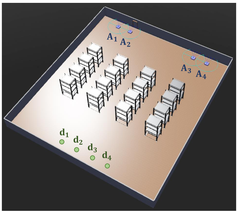
(a) Side view

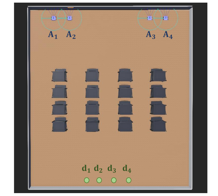
(b) Top-down view

Figure 3: Environment scenario with $4$ agents and $4$ obstacles in a warehouse setting. The agents $\{A_{i}\}_{i=1}^{4}$ represent robots, the obstacles represent rectangular shelves of size $1\times 4$, and the green circles $\{{\mathbf{d}}_{i}\}_{i=1}^{4}$ represent the goal positions. (a) Side view of the environment. (b) Top-down view of the environment.

In real-world applications, it is neither practical nor realistic to have solutions that abruptly change over “time”. It is standard to impose a soft constraint that penalizes the inverse objective function with the deviation of its solution from the one obtained at the previous “time” [50]. The resulting discrete time-varying optimization problem with proximal regularization (except for the initial problem) becomes

$$\min_{\boldsymbol{\theta}_{o}}\leavevmode\nobreak\ g({\mathbf{S}},{\mathbf{D}},\alpha^{(0)},\boldsymbol{\theta}_{o})$$ (14)

$$\min_{\boldsymbol{\theta}_{o}}\leavevmode\nobreak\ g({\mathbf{S}},{\mathbf{D}},\alpha^{(k)},\boldsymbol{\theta}_{o})+\frac{\eta\|\boldsymbol{\theta}_{o}-\boldsymbol{\theta}_{o}^{(k-1)*}\|}{2\Delta\alpha}$$ (15)

for $k=1,2,\ldots$, where $\boldsymbol{\theta}_{o}^{(k-1)*}$ is a local minimum of problem (15) at iteration $k-1$ and $\eta$ is a regularization parameter that weighs the regularization term to the inverse objective function. The first term in (15) denotes the inverse objective function, while the second term in (15) denotes the deviation of the decision variable $\boldsymbol{\theta}_{o}$ at current iteration $k$ from the local minimum at previous iteration $k-1$. By taking the derivative and using the first-order stationary condition, the local minimum of (15) at iteration $k$ satisfies

$$\nabla_{\boldsymbol{\theta}_{o}}g({\mathbf{S}},{\mathbf{D}},\alpha^{(k)},\boldsymbol{\theta}_{o}^{(k)*})\!+\!\eta\frac{\boldsymbol{\theta}_{o}^{(k)*}\!-\!\boldsymbol{\theta}_{o}^{(k-1)*}}{\Delta\alpha}\!=\!0,$$ (16)

where the first term represents the inverse objective gradient and the second term represents the change of the local minimum at two successive iterations. When the step-size approaches zero $\Delta\alpha\to 0$, the continuous limit of (16) becomes the ordinary differential equation (ODE) as

$$\eta\boldsymbol{\theta}_{o}^{\prime}(\alpha)\!=\!-\!\nabla_{\boldsymbol{\theta}_{o}}g({\mathbf{S}},{\mathbf{D}},\alpha,\boldsymbol{\theta}_{o}(\alpha)),\leavevmode\nobreak\ \boldsymbol{\theta}_{o}(0)\!=\!\boldsymbol{\theta}_{o}^{(0)*},$$ (17)

where $\boldsymbol{\theta}_{o}(\alpha)$ is a dynamic function of $\alpha$ and $\boldsymbol{\theta}^{\prime}_{o}(\alpha)$ is the derivative of $\boldsymbol{\theta}_{o}(\alpha)$ w.r.t. $\alpha$. The solution of the preceding ODE (17) is a local minimum trajectory of the continuous time-varying optimization problem with proximal regularization [cf. (14)-(15) with $\Delta\alpha\to 0$]. When $\eta=0$, the ODE (17) reduces to the first-order stationary condition of the time-varying optimization problem (13). Given the initial point $\boldsymbol{\theta}_{o}(0)$, we assume there exists a local minimum trajectory ${\mathcal{T}}(\alpha)$ [Def. 1] satisfying that $\boldsymbol{\theta}_{o}(\alpha)-{\mathcal{T}}(\alpha)$ lies in a compact set $D$ for $\alpha\geq 0$. With these preliminaries in place, we formally show the convergence of the proposed coordinated optimization method in the following theorem.

Theorem 1.

Consider the non-convex time-varying optimization problem (13) satisfying Assumption 1 w.r.t. $C_{L}$ and the policy gradient in (10) satisfying Assumption 2 w.r.t. $\varepsilon$. Let $\boldsymbol{\theta}_{o}(\alpha)$ be a solution of the ODE (17) with the regularization parameter $\eta$ and $\big{\{}\boldsymbol{\theta}_{o}^{(k)}\big{\}}_{k}$ be the discrete sequence of the generative parameters updated by the proposed method, where the step-size of the policy gradient ascent is $\Delta\beta=\Delta\alpha/\eta$ [cf. (10)]. Let also the initial $\boldsymbol{\theta}_{o}^{(0)}=\boldsymbol{\theta}_{o}(0)$ be a local minimum of $g({\mathbf{S}},{\mathbf{D}},0,\boldsymbol{\theta}_{o})$. Then, for any $\epsilon>0$ and “time” $T$, there exists a step-size $\Delta\alpha$ such that

$$\|\boldsymbol{\theta}_{o}^{(k)}-\boldsymbol{\theta}_{o}(\alpha^{(k)})\|\leq\epsilon+C\varepsilon$$ (18)

for all iterations $k=1,\ldots,\lfloor T/\Delta\alpha\rfloor$, where $C$ is a constant depending on $C_{L}$, $\eta$ and $T$ [cf. (32)].

Proof.

See Appendix A. ∎

Theorem 1 states that the proposed co-optimization method converges to the local minimum trajectory of a time-varying non-convex optimization problem, i.e., the solution of the ODE (17), up to a limiting error neighborhood. The latter consists of two additive terms: i) the first term $\epsilon$ is the desired error, which can be arbitrarily small; ii) the second term is proportional to the accuracy of the policy gradient $\varepsilon$, which becomes null as the policy gradient approaches the true gradient. The update step-sizes of the navigation policy $\Delta\alpha$ and the generative model $\Delta\beta=\Delta\alpha/\eta$ depend on the Lipschitz constant $C_{L}$, the regularization parameter $\eta$, the desired error $\epsilon$ and the time interval $T$ [cf. (32)]. This indicates that a more accurate solution, i.e., a smaller $\epsilon$, requires a smaller step-size $\Delta\alpha$, which may slow down the training procedure. This result characterizes the convergence behavior of the proposed method and interprets its inherent working mechanism, i.e., performing the proposed method is equivalent to tracking the local minimum trajectory of an associated time-varying non-convex optimization problem.

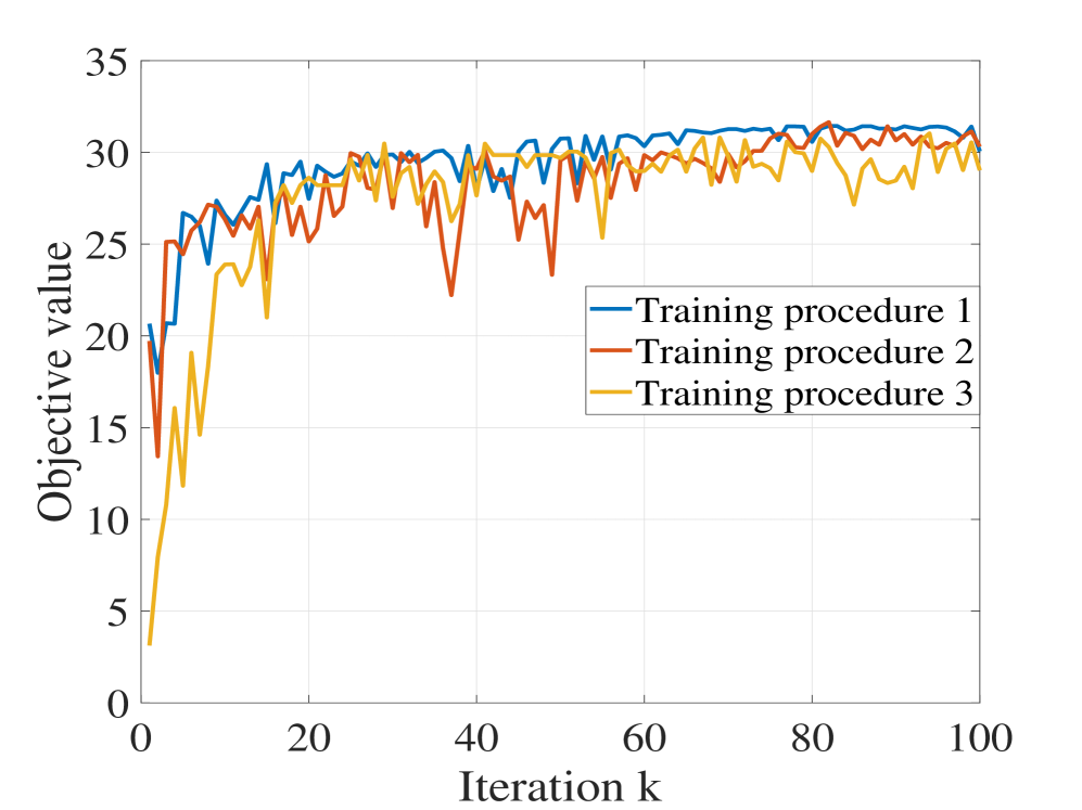
(a)

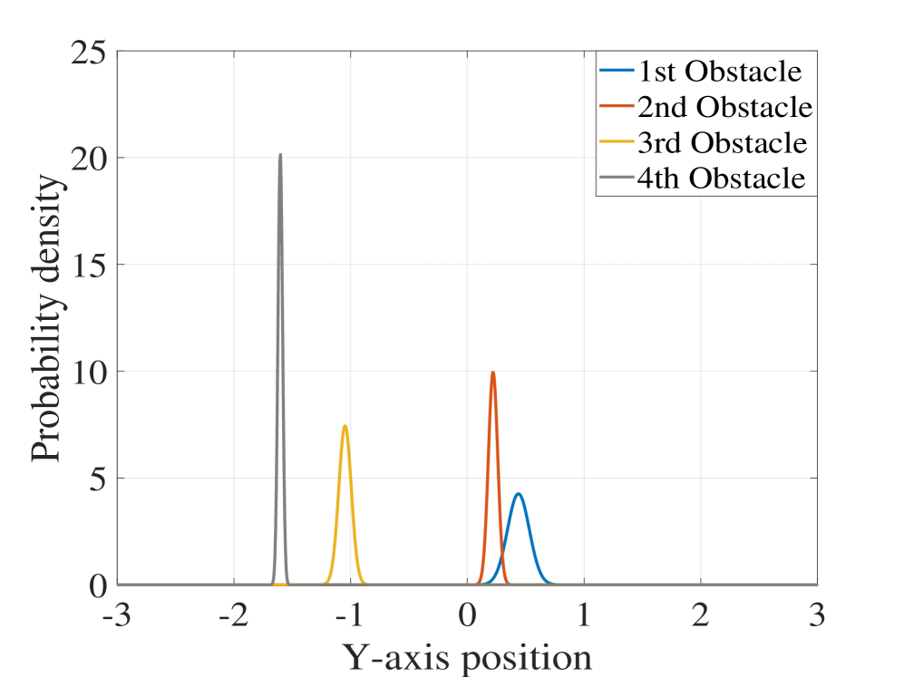
(b)

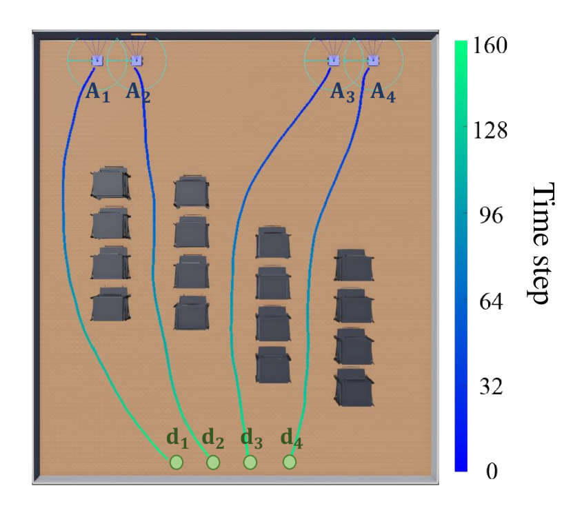
(c)

Figure 4: Proof of concept for agent-environment coordinated optimization. (a) Training procedure of coordinated optimization method. (b) Generative distributions for $4$ obstacles. (c) Obstacle layout produced by the generative model and agent trajectories controlled by the navigation policy. Blue-to-green lines are trajectories of agents and the color bar represents the time scale.

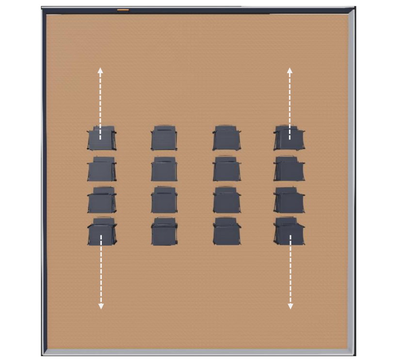
(a) Environment I

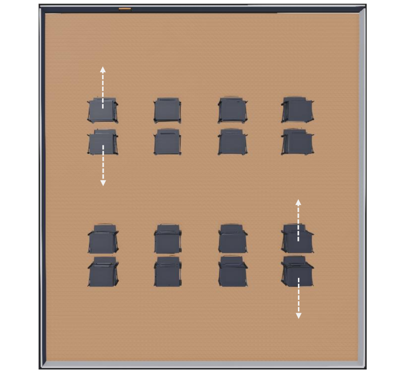
(b) Environment II

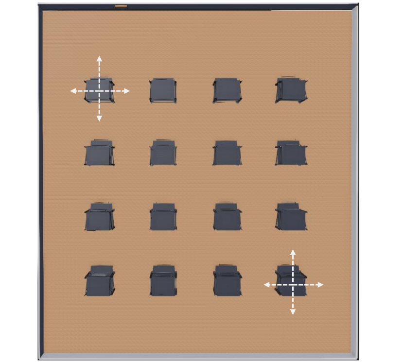
(c) Environment III

Figure 5: Three environments in Section V-C. (a) Environment I with $4$ obstacles of size $1\times 4$. (b) Environment II with $8$ obstacles of size $1\times 2$. (c) Environment III with $16$ obstacles of size $1\times 1$.

V Experiments

In this section, we evaluate the coordinated optimization method. First, we conduct a proof of concept to demonstrate the effectiveness of our approach. Then, we show how our approach improves the multi-agent navigation performance in a warehouse setting. Lastly, we characterize the role of the environment on the multi-agent system through our method and show that an appropriate obstacle layout can provide “positive” guidance for agents, beyond “negative” interference and obstruction as in conventional beliefs. This finding has not been explored thus far, which highlights the importance of establishing a symbiotic agent-environment co-evolved system.

V-A Implementation Details

The agents and obstacles are modeled by their positions $\{{\mathbf{p}}_{ai}\}_{i=1}^{n}$, $\{{\mathbf{p}}_{oj}\}_{j=1}^{m}$ and velocities $\{{\mathbf{v}}_{ai}\}_{i=1}^{n}$. For multi-agent navigation, each agent observes its own state (i.e., position and velocity), communicates with neighboring agents, and generates the desired velocity with received neighborhood information. We integrate an acceleration-constrained mechanism for position changes and an episode ends if all agents reach destinations or episode times out. The maximal acceleration is $1m/s^{2}$, the maximal velocity is $1.5m/s$, the communication radius is $2m$, the maximal time is $500$ steps and each time step is $0.05s$. The goal is to make agents reach destinations quickly while avoiding collision. We define the reward function as

$$r_{ai}^{(t)}=\Big{(}\frac{{\mathbf{p}}_{ai}^{(t)}-{\mathbf{d}}_{i}}{\|{\mathbf{p}}_{ai}^{(t)}-{\mathbf{d}}_{i}\|_{2}}\cdot\frac{{\mathbf{v}}_{ai}^{(t)}}{\|{\mathbf{v}}_{ai}^{(t)}\|_{2}}\Big{)}\|{\mathbf{v}}_{ai}^{(t)}\|_{2}+C_{p}^{(t)}$$ (19)

at time step $t$. The first term rewards fast movement to the goal position at the desired orientation, and the second term represents the collision penalty. We parameterize the navigation policy with a single-layer GNN, where the message aggregation and feature update functions are multi-layer perceptrons (MLPs). We train the policy using PPO [51].

For the environment optimization, the generative model produces $m$ independent generative distributions, each of which controls the configuration (e.g., position and size) of one obstacle. We consider generative distributions as truncated Gaussian distributions – see Appendix B-C, where the dimension, lower bound and upper bound depend on specific environment settings. For example in Fig. 3(a), each obstacle represents a shelf in the warehouse. The obstacle position on the $x$-axis is fixed and that on the $y$-axis can be adjusted in $[-4,4]$ by sliding it along a linear track. The generative distribution is a $1$-D truncated Gaussian distribution with a lower bound $-4$ and an upper bound $4$. We parameterize the generative model with a DNN of $3$ layers with $(32,64,32)$ hidden units and ReLU nonlinearity, to produce parameters that specify the generative distributions.

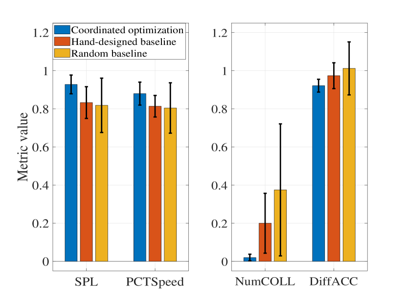
(a)

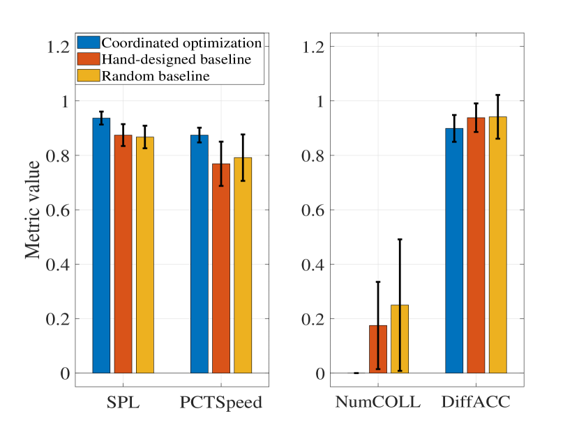
(b)

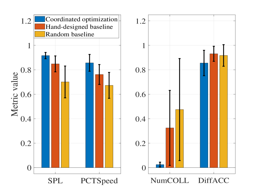
(c)

Figure 6: Performance of agent-environment coordinated optimization method compared with two baselines in three environments. A higher value of SPL or PCTSpeed represents a better performance, while a lower value of NumCOLL or DiffACC represents better safety or more comfort. (a) Environment I. (b) Environment II. (c) Environment III.

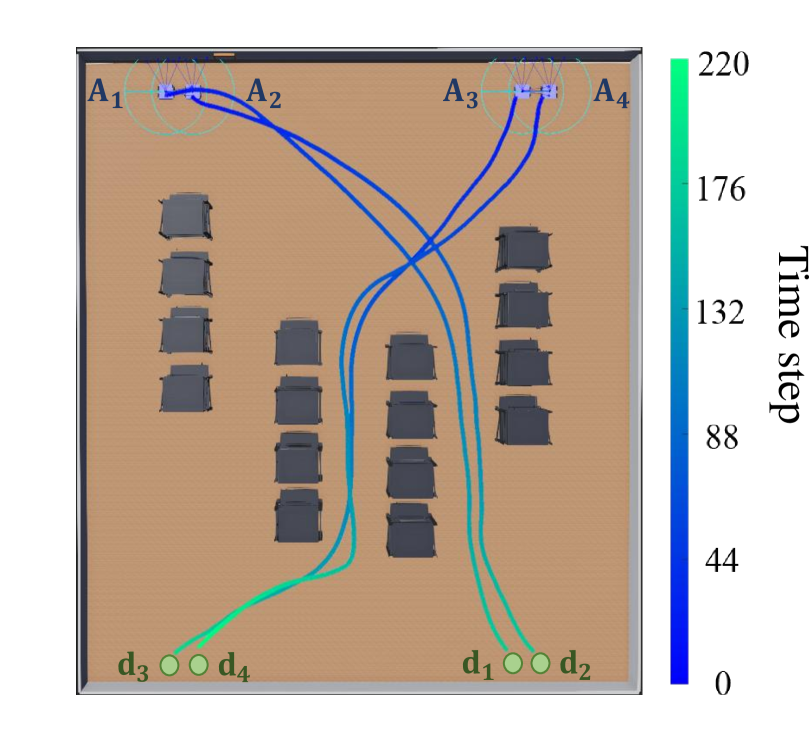
(a) Optimized Environment I

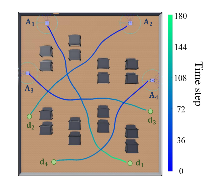
(b) Optimized Environment II

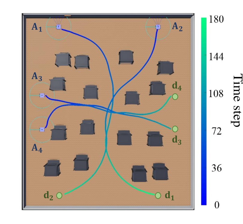
(c) Optimized Environment III

Figure 7: Examples of agent-environment coordinated optimization in three environments. Blue robots $\{A_{i}\}_{i=1}^{4}$ represent agents at initial positions, green circles $\{{\mathbf{d}}_{i}\}_{i=1}^{4}$ represent goal positions, and black boxes represent obstacles (rectangular shelves). Color lines from blue to green are agent trajectories and the color bar represents the time scale. (a) Optimized Environment I. (b) Optimized Environment II. (c) Optimized Environment III.

We employ Webots as our 3D simulation platform and leverage its physics engine to simulate real-world dynamics. Each agent is modeled as an omni-directional robot that has four wheels [52]. They are configured with fine-tuned frictional coefficients governing the interaction between their wheels and the ground surface. The collision detection is based on the mesh geometry that is imposed on the entities within the simulator. Each robot has a receiver and an emitter module to broadcast and receive the state information from its neighboring robots for communication. The low-level control is handled by Model Predictive Control (MPC), which converts the navigation policy output to each wheel’s speed using inverse kinematics.

V-B Proof of Concept

First, we conduct a proof of concept with $n=4$ agents and $m=4$ obstacles. We consider an environment of size $10\times 12$ in the warehouse setting as depicted in Fig. 3. The agents are robots of size $0.4$, which are initialized randomly in the starting region ${\mathcal{S}}$ and tasked towards the destination region ${\mathcal{D}}$. The obstacles are rectangular shelves of size $1\times 4$, which are distributed in the obstacle region $\Delta$. The obstacle positions on the $x$-axis are fixed, yet are configurable on the $y$-axis in the range of $[-4,4]$ to improve the navigation performance.

Fig. 4(a) shows the performance during training. We see that the objective value increases with the number of iterations and approaches a stationary condition, which corroborates the convergence analysis in Theorem 1. Fig. 4(b) plots the generative distributions for four obstacles, respectively, which demonstrate how the generative model places the obstacles in the environment. First, we note that the standard deviation of the distribution is small, i.e., the probability density concentrates in a small region. This indicates that there is little variation in the environment generation (hence, the obstacle position and the resulting performance). Second, the generative model produces an irregular obstacle layout that differs from the hand-designed one, which implies that structure irregularity is capable of providing navigation help for the multi-agent system. Fig. 4(c) shows the agent trajectories controlled by our navigation policy in the generated environment, where agents move smoothly from initial positions to their destinations without collision.

V-C Performance Evaluation

We further evaluate our approach in three different cluttered environments that resemble a warehouse setting:

• Environment I is equipped with $m=4$ obstacles of size $1\times 4$ – see Fig. 5(a). The obstacle positions on the $x$-axis are fixed, and those on the $y$-axis can be re-configured in the range $[-4,4]$.

• Environment II is equipped with $m=8$ obstacles of size $1\times 2$ – see Fig. 5(b). The obstacle positions on the $x$-axis are fixed, and those on the $y$-axis can be re-configured in the range $[-4,0]$ or $[0,4]$.

• Environment III is equipped with $m=16$ obstacles of size $1$$\times$$1$ – see Fig. 5(c). The obstacle positions can be re-configured along both $x$- and $y$-axes in a neighborhood of size $2\times 2$.

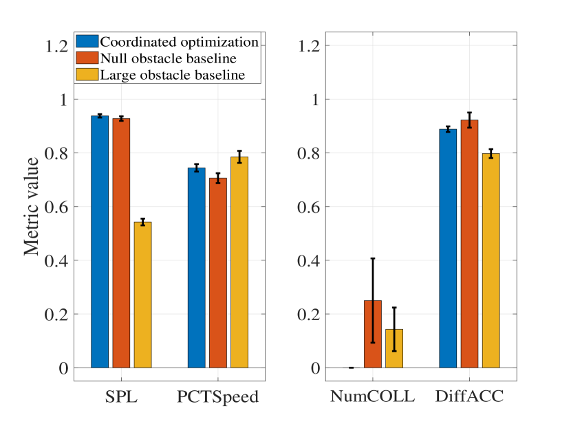
(a)

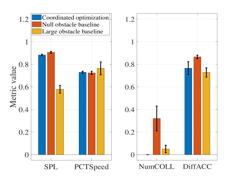
(b)

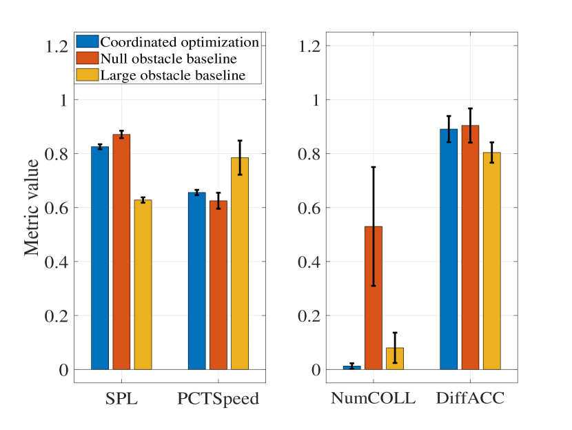
(c)

Figure 8: Performance of agent-environment coordinated optimization compared with two baseline scenarios in the circular setting with different numbers of agents. A higher value of SPL or PCTSpeed represents a better performance, while a lower value of NumCOLL or DiffACC represents better safety or more comfort. (a) $n=8$ agents. (b) $n=12$ agents. (c) $n=16$ agents.

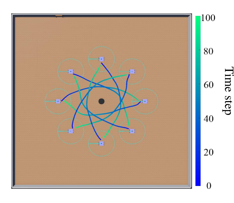
(a) Environment with $8$ agents

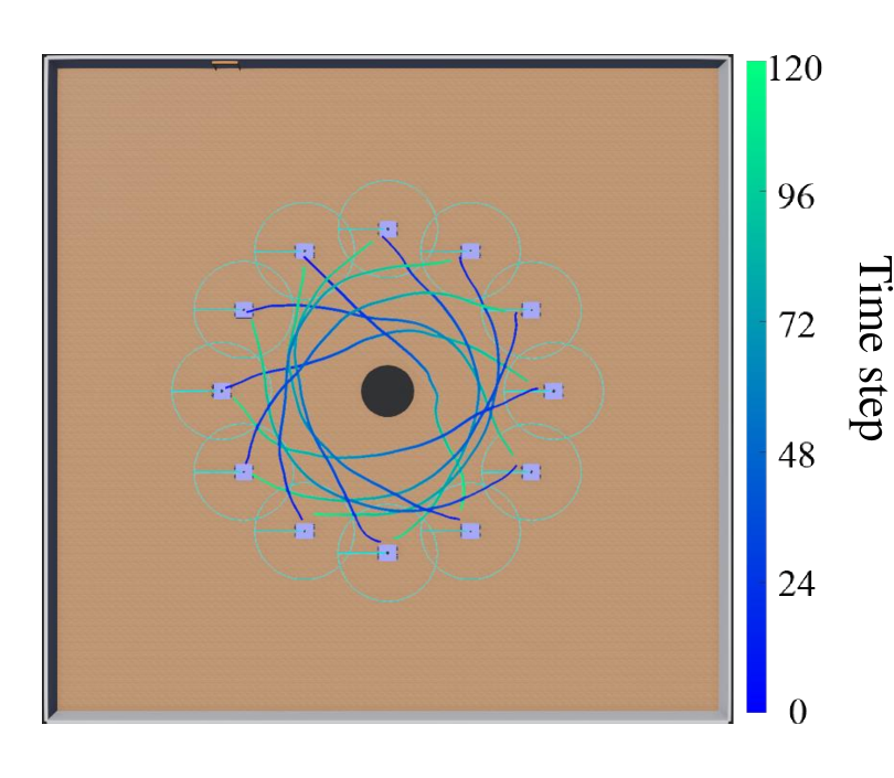
(b) Environment with $12$ agents

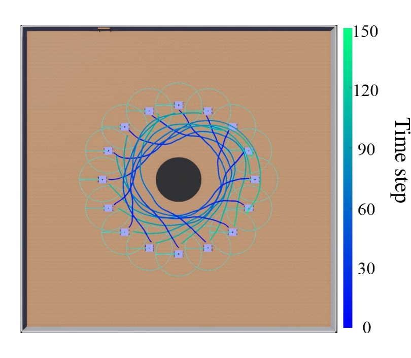
(c) Environment with $16$ agents

Figure 9: Examples of agent-environment coordinated optimization in the circular setting with different numbers of agents. Blue robots $\{A_{i}\}_{i=1}^{n}$ represent agents at initial positions, green circles $\{{\mathbf{d}}_{i}\}_{i=1}^{n}$ represent goal positions, and the solid black circle represents the obstacle. Color lines from blue to green are agent trajectories and the color bar represents the time scale. (a) $n=8$ agents. (b) $n=12$ agents. (c) $n=16$ agents.

We measure the navigation performance of the multi-agent system with four metrics: (i) Success weighted by Path Length (SPL) [53], (ii) the percentage to the maximal speed (PCTSpeed), (iii) the average number of “collisions” (NumCOLL), and (iv) the average finite difference of the acceleration (DiffACC). SPL is a stringent measure that combines navigation success rate with path length overhead, and has been widely used as a primary quantifier in comparing navigation performance [53, 54, 55]. PCTSpeed represents the ratio of the average speed to the maximal one, and provides complementary information regarding the moving speed along trajectories. These two metrics normalize their values to $[0,1]$, where a higher value represents a better performance. NumCOLL counts the number of “collisions” averaged over agents, where an agent is considered collided at time $t$ if it is within the safety range of another agent or obstacle, and measures the safety of the multi-agent system. DiffACC represents the change of agents’ acceleration averaged over time steps, and indicates the comfort (smoothness) of the navigation procedure [56, 57]. For the latter two metrics, a lower value represents a better performance, i.e., better safety and more comfort. Our results are averaged over $10$ random tasks (initial and goal positions) with $10$ random trials for a total of $100$ runs.

Fig. 6 shows the performance of the coordinated optimization method. We consider two baselines for comparison: the widely-used hand-designed environment in Fig. 5 and the randomly generated environment. Our method outperforms the baselines consistently with the highest SPL and PCTSpeed and the lowest NumCOLL and DiffACC, and maintains a good performance across different environments. We attribute this behavior to the fact that the generative model adapts the obstacle layout to alleviate environment restrictions, based on which the navigation policy tunes the agent trajectories to improve the system performance. The performance improvement is emphasized as the environment structure becomes more complex from Environment I with $4$ obstacles to Environment III with $16$ obstacles. This is because as multi-agent navigation gets more challenging, agents benefit more from compatible environments.

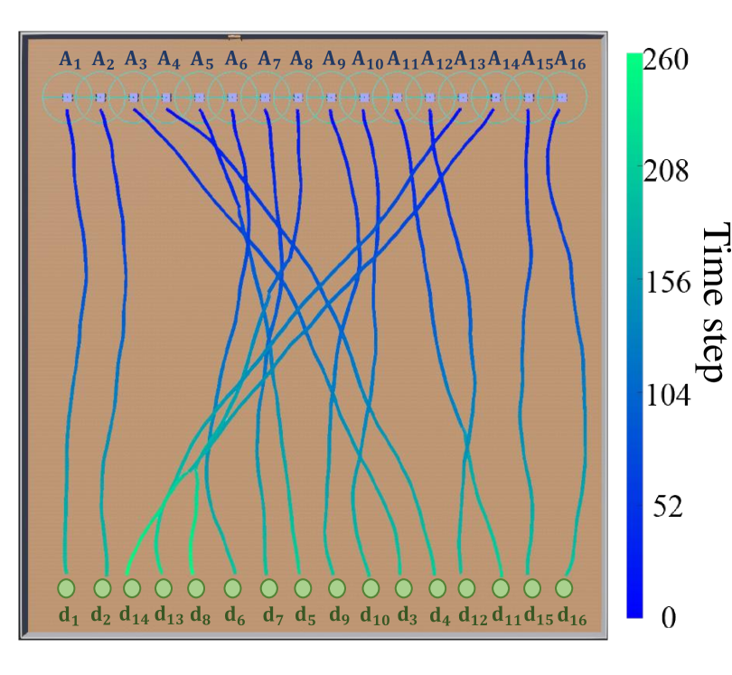
(a) Environment with obstacle radius $0$

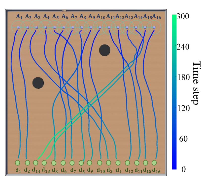
(b) Environment with obstacle radius $0.5$

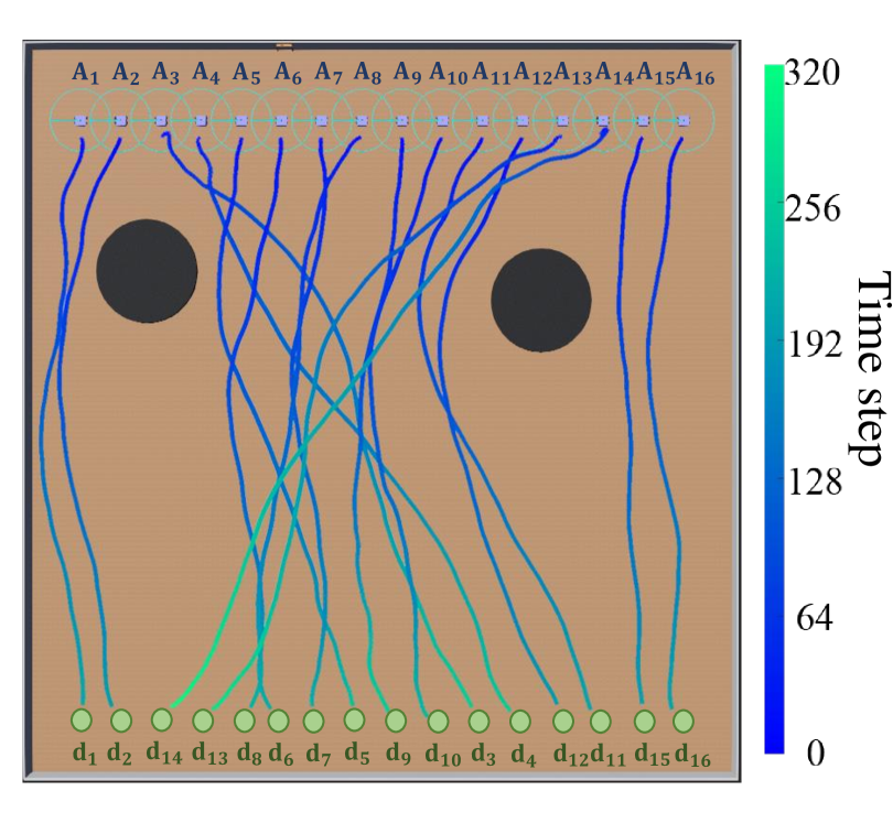
(c) Environment with obstacle radius $1$

Figure 10: Examples of agent-environment coordinated optimization in Case I of the randomized setting with different obstacle radii. Blue robots $\{A_{i}\}_{i=1}^{16}$ represent agents at initial positions, green circles $\{{\mathbf{d}}_{i}\}_{i=1}^{16}$ represent goal positions, and solid black circles represent obstacles. Color lines from blue to green are agent trajectories and the color bar represents the time scale. (a) Null radius $r=0$. (b) Radius $r=0.5$. (c) Radius $r=1$.

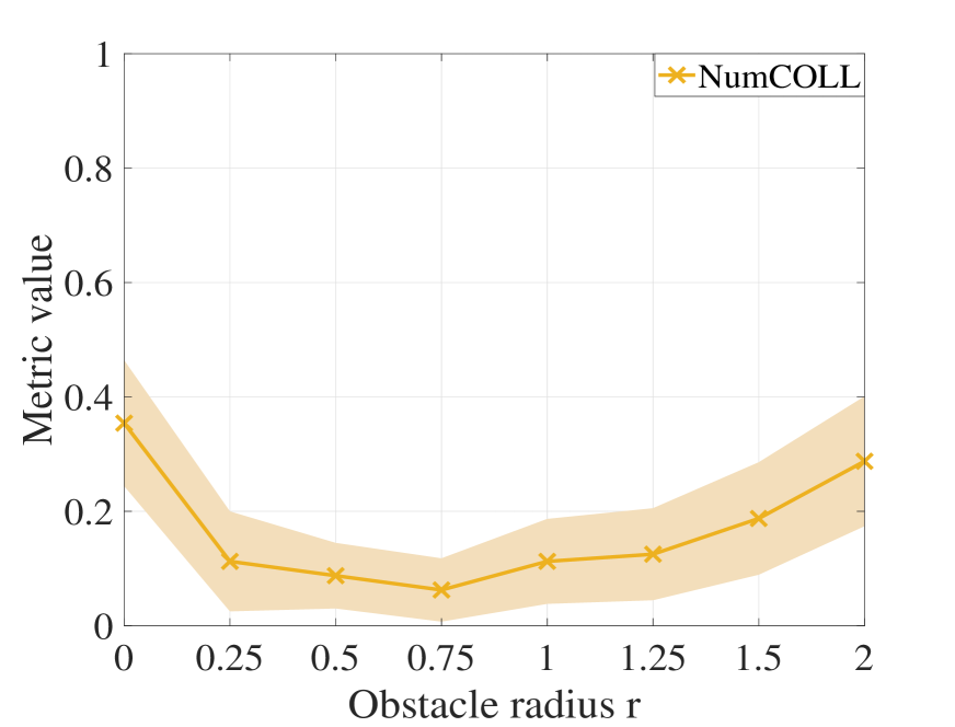
(a)

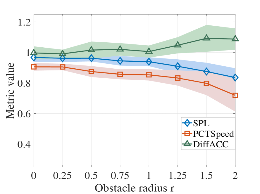
(b)

Figure 11: Performance of agent-environment coordinated optimization in Case I of the randomized setting with different obstacle radii. A higher value of SPL or PCTSpeed represents a better performance, while a lower value of NumCOLL or DiffACC represents better safety or more comfort.

Fig. 7 displays examples of the agent-environment co-optimization in the three Environments I-III, respectively. We see that: (i) The generative model produces different obstacle layouts based on different navigation tasks. The resulting environment exhibits an irregular structure that differs from the hand-designed one, which helps the multi-agent system improve its navigation performance. (ii) The generated environment not only creates obstacle-free pathways for agent navigation, but also prioritizes these pathways by structure irregularity for agent deconfliction. For example in Fig. 7(c), while the navigation tasks of $A_{1}$, $A_{2}$ and $A_{3}$, $A_{4}$ are symmetric, the generative model produces an obstacle layout with non-symmetric pathways to avoid potential collisions among agents. (iii) The navigation policy is compatible with the generative model and selects the optimal trajectories in the generated environment, moving the agents smoothly towards their destinations. (iv) The navigation policy strives to move agents as a team (or sub-team) so that they remain connected, and only separates them as a last resort. This is because the agents rely on their neighborhood information to make collectively meaningful decisions in the decentralized setting.

These results indicate that our approach establishes a symbiotic agent-environment system, where the environment and the agents rely on and adapt to each other; ultimately, yielding an improved navigation performance.

V-D Hindrance vs. Guidance

Next, we investigate the role played by the environment in multi-agent navigation by leveraging our coordinated optimization method. Obstacles are typically viewed as “negative” elements that create inaccessible areas or obstruct agent pathways (and hinder ideal trajectories). However, we hypothesize that an appropriate obstacle layout can have “positive” effects by forming designated collision-free zones for the agents to follow. Such an arrangement can provide navigation guidance and help de-conflict agents, especially in dense settings. The following experiments aim to verify this hypothesis and to capture the relationship between the environment and the agents. I.e., we are interested in uncovering an implicit trade-off between hindrance and guidance roles that the environment may take on.

We consider two environment settings motivated by traffic system design for safe navigation, to glean insights into the hindrance-guidance trade-off.

Circular setting. The environment is of size $8\times 8$, where agents are initialized along a circle – see Fig. 9. The goal of the navigation policy is to cross-navigate the agents towards the opposite side while avoiding collisions among each other, and the goal of the generative model is to determine the radius of the circular obstacle at the origin $(0,0)$ to de-conflict the multi-agent navigation. An obstacle with a large radius reduces the area of reachable space for the agents and may degrade the navigation performance, while an obstacle with a small radius provides a negligible guiding effect and may not prevent agent conflicts (e.g., all agents attempt to move along the shortest but intersecting trajectories). We explore this trade-off by performing the agent-environment co-optimization to find the optimal obstacle radius.

Fig. 8 shows the performance of the coordinated optimization method with different numbers of agents $n\in\{8,12,16\}$. We consider two baseline scenarios for comparison: a null obstacle of radius $0$ and a large obstacle of radius $2$. We see that the presence of the obstacle with an appropriate radius improves the agents’ performance with a significantly lower NumCOLL. This improvement increases with the number of agents, which can be explained by the fact that a more cluttered system requires more guidance from the obstacle for agent deconfliction. The baseline scenario with a null obstacle achieves a comparable SPL / PCTSpeed but increases the NumCOLL, despite no hindrance along agent trajectories. This is because the agents have to coordinate their navigation trajectories with only neighborhood information at hand, and receive no guidance from the obstacle. The latter makes it challenging to de-conflict, especially in a cluttered environment with a large number of agents. The baseline scenario with a large obstacle results in a lower SPL and a slightly higher NumCOLL because it reduces the amount of reachable space and imposes more restrictions on the feasible solution. The latter blocks the shortest pathways and forces the agents to move along inefficient trajectories towards destinations.

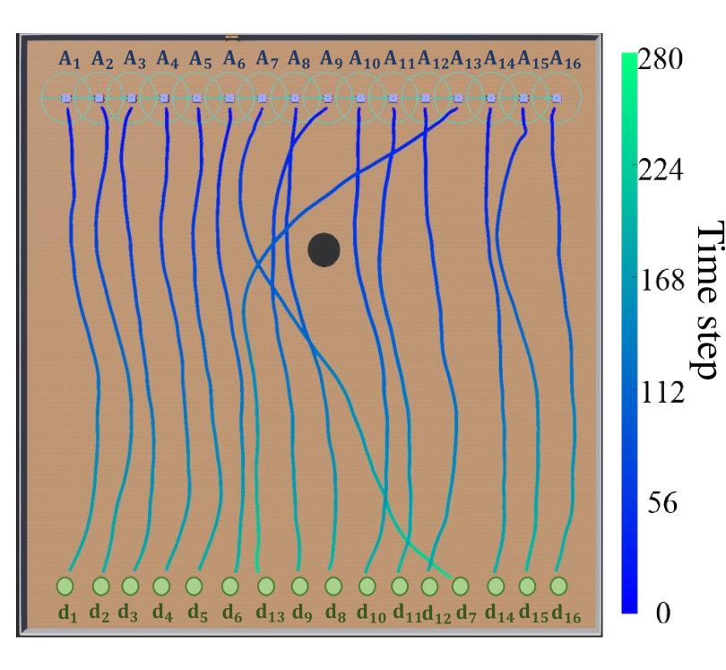
(a) Environment with $4$ random agents

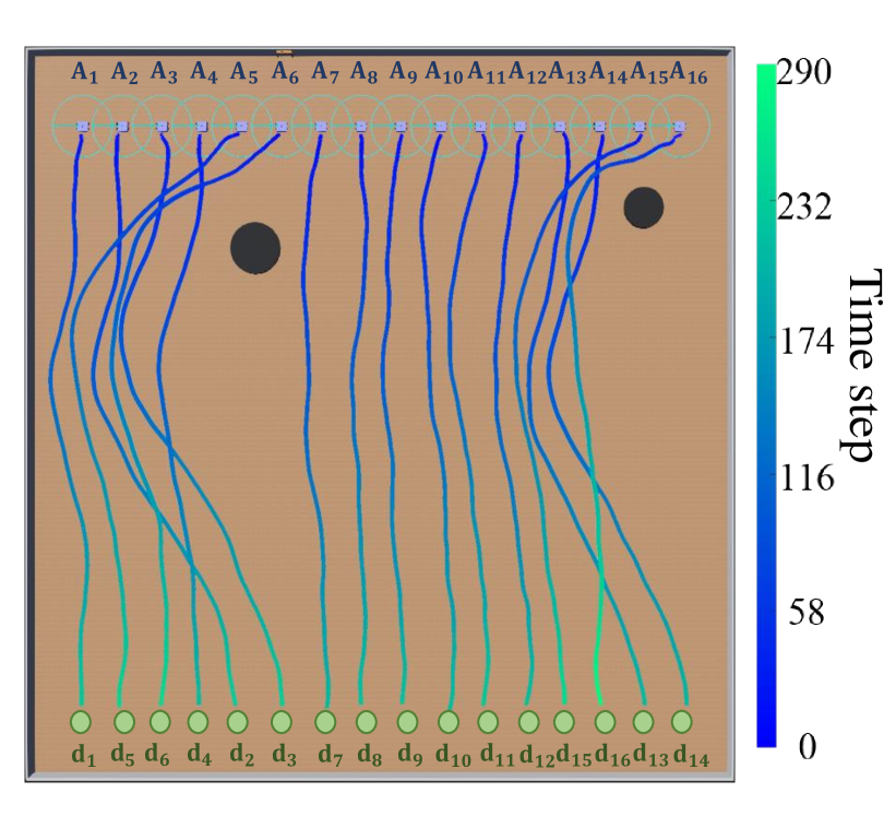
(b) Environment with $8$ random agents

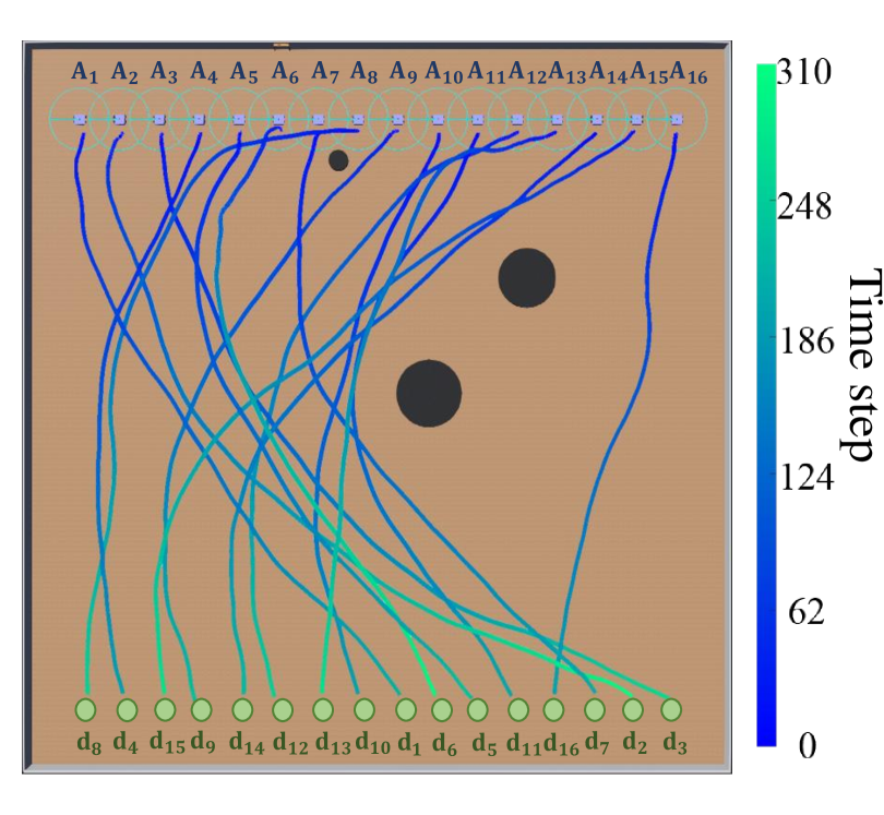
(c) Environment with $16$ random agents

Figure 12: Examples of agent-environment coordinated optimization in Case II of the randomized setting with different numbers of random agents. Blue robots $\{A_{i}\}_{i=1}^{16}$ represent agents at initial positions, green circles $\{{\mathbf{d}}_{i}\}_{i=1}^{16}$ represent goal positions, and solid black circles represent obstacles. Color lines from blue to green are agent trajectories and the color bar represents the time scale. (a) $\eta=4$ random agents. (b) $\eta=8$ random agents. (c) $\eta=16$ random agents.

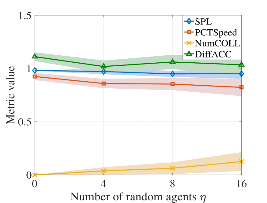
(a)

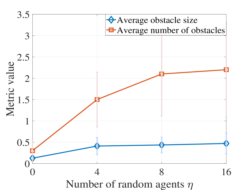
(b)

Figure 13: (a) Performance of agent-environment coordinated optimization in Case II of the randomized setting with different numbers of random agents $\eta$. A higher value of SPL or PCTSpeed represents a better performance, while a lower value of NumCOLL or DiffACC represents better safety or more comfort. (b) Average obstacle radius and average number of obstacles determined by coordinated optimization method with different numbers of random agents $\eta$.

Fig. 9 plots the obstacle radius of the generative model and the agent trajectories of the navigation policy. The obstacle radius generated by the proposed method increases with the number of agents $n$. For a small $n$, the agents are sparsely distributed and need less guidance from the obstacle for deconfliction; hence, leading to a small radius that does not hinder agent pathways. For a large $n$, the agents are densely distributed and require more help from the obstacle for coordination; hence, leading to a large radius that guides the agents moving clockwise towards destinations.

Randomized setting. The environment is of size $18\times 18$ with $16$ starting positions $\{{\mathbf{s}}_{i}\}_{i=1}^{16}$ on the top and $16$ goal positions $\{{\mathbf{d}}_{i}\}_{i=1}^{16}$ on the bottom – see Fig. 10. There are $16$ agents $\{A_{i}\}_{i=1}^{16}$ initialized at $\{{\mathbf{s}}_{i}\}_{i=1}^{16}$ and tasked towards $\{{\mathbf{d}}_{i}\}_{i=1}^{16}$ in order, i.e., agent $A_{i}$ is initialized at ${\mathbf{s}}_{i}$ and tasked towards ${\mathbf{d}}_{i}$ for $i=1,\ldots,16$. The goal of the navigation policy is to move the agents to their goal positions while avoiding collision among each other, and the goal of the generative model is to determine the obstacle layout between starting and goal positions to facilitate safe navigation. An environment with a large number of obstacles or a large obstacle size hinders agent pathways, while an empty environment might not provide enough guidance for effective agent deconfliction. By leveraging agent-environment co-optimization, we explore this trade-off to find the optimal obstacle layout for different navigation cases.

Case I. We consider an environment with $2$ circular obstacles, where the obstacle radius varies in $[0,2]$. We randomly switch the initial and goal positions of $8$ agents, while keeping the other $8$ agents unchanged – see Fig. 10(a). The generative model determines the optimal positions of the obstacles that de-conflict the agents while avoiding hindering their pathways, striking a balance between the guidance and the hindrance roles.

Fig. 11(a) shows that NumCOLL first decreases with the obstacle radius $r$, and then increases for large radii $r$. The former is because an initial increase in $r$ allows the presence of the obstacles in an empty environment, which provides the operation space for the coordinated optimization method to de-conflict the agents with an appropriate obstacle layout. The result for large $r$ corresponds to the fact that further increasing $r$ occupies more collision-free space but provides little additional guidance, leading to an increased NumCOLL. Fig. 11(b) shows that SPL, PCTSpeed decrease and DiffACC increases slightly with the obstacle radius $r$, while all maintaining a good performance. This slight degradation is because (i) increasing $r$ reduces the reachable space in the environment and (ii) some agents make a detour under the obstacle guidance to avoid collision with the other agents.

Fig. 10 plots examples of how our method optimizes the obstacle positions with different obstacle radii. We see that different positions and sizes of the obstacles have different impact on the agents’ trajectories, and the obstacles are typically placed around the intersections of the agents’ trajectories to separate the crowd and de-conflict the agents. For example, with no obstacle in Fig. 10(a), agents $A_{12}$, $A_{13}$, $A_{14}$ all attempt to move fast along short paths, which increases the risk of agent collisions. With the presence of obstacles in Fig. 10(c), agents $A_{13}$, $A_{14}$ are guided to slow down and make a detour for agent $A_{12}$ to avoid potential collisions.

Case II. We consider an environment with at most $4$ circular obstacles. We randomly switch the initial and goal positions of $\eta$ agents, where $\eta\in[0,16]$ represents the randomness of the navigation task, while keeping the rest $16-\eta$ agents unchanged – see Fig. 12. The generative model determines: (i) the number of obstacles presented in the environment; (ii) the obstacle radii and (iii) the obstacle positions, to de-conflict the agents while avoiding blocking their pathways.

Fig. 13(a) shows the performance with different numbers of random agents $\eta$. We see that the proposed method maintains a good performance across varying agent randomness, highlighting its capacity in handling different navigation scenarios. SPL and PCTSpeed decrease and NumCOLL increases slightly with the increasing of agent randomness because the navigation task becomes more challenging as the initial and goal positions of the agents get more random. Fig. 13(b) plots the average obstacle size and the average number of presented obstacles with different numbers of random agents $\eta$. Both values increase with the navigation randomness, while the increasing rates decrease as $\eta$ becomes large. The former is because when the randomness is small, the agents are capable of handling the deconfliction and need little help from the obstacles; when the randomness increases and the system becomes cluttered, the agents need more or larger obstacles to provide guidance for deconfliction. The latter is because as the obstacle number or radius reaches a saturated level, it has sufficient capacity to guide the agents and thus, reduces the increasing rate. Fig. 12 plots examples of how our approach optimizes the obstacle layout for agents. For one thing, it guides the agent crowd and sorts out the navigation randomness, e.g., it guides a subset of agents to slow down and take a detour to make way for the other agents. For another, it does not take too much collision-free space and avoids hindering agent pathways.

The above results demonstrate that the obstacles are not always “bad”, but instead, can play “good” guidance roles for the agents with an appropriate layout. These insights can be used for traffic design to facilitate safe and efficient navigation.

VI Conclusion

This paper proposed an agent-environment coordinated optimization framework for multi-agent systems. The problem comprises two components: (i) multi-agent navigation and (ii) environment optimization, where the former seeks a navigation strategy that moves agents from origins to destinations, and the latter seeks a design scheme that generates an appropriately accommodating environment (w.r.t the task at hand). These components must then be optimized in a joint manner such that an overarching objective is achieved (in our case: improved navigation performance). We solved this problem by alternating the optimization of the multi-agent navigation policy and an environment generative model. We followed a model-free learning-based approach, and, towards this end, introduced a novel combination of reinforcement learning (through an actor-critic mechanism) and unsupervised learning (through policy gradient ascent) for coordinated optimization. Furthermore, we analyzed the convergence of our method by exploring its relation with an associated time-varying non-convex optimization problem and ordinary differential equations. Numerical results corroborated theoretical findings and showed the benefit of co-optimization over baselines, i.e., the agent-environment co-optimization finds agent-friendly environments and efficient navigation trajectories. Finally, we investigated the role of the environment in multi-agent navigation to show that it does not just impose physical restrictions, but can also provide guidance for agent deconfliction if designed appropriately. The latter explores an inherent relationship between the environment and agents in a way previously unaddressed.

In future work, we are interested in adding constraints to the agent-environment co-optimization framework, to represent real-world physical limitations either on the multi-agent system (e.g., non-holonomicity) or on the environment (e.g., occupied space), and plan on developing algorithms to solve such constrained co-optimization problems. Moreover, we plan to use our co-optimization method for higher-dimensional multi-agent tasks, such as multi-drone navigation in 3-dimensional environments or manipulator motion planning in high-dimensional configuration spaces.

Appendix A Proof of Theorem 1

First, from Theorem 3.3 in [58], the ODE (17) has a unique solution $\boldsymbol{\theta}_{o}(\alpha)$ starting from the point $\boldsymbol{\theta}_{o}^{(0)}=\boldsymbol{\theta}_{o}(0)$. Then, we show the discrete parameters $\big{\{}\boldsymbol{\theta}_{o}^{(k)}\big{\}}_{k}$ of the proposed method converges to this solution $\boldsymbol{\theta}_{o}(\alpha)$.

From Taylor’s theorem, we can expand the ODE solution $\boldsymbol{\theta}_{o}(\alpha)$ at $\alpha^{(k+1)}$ as

$$\boldsymbol{\theta}_{o}(\alpha^{(k+1)})=\boldsymbol{\theta}_{o}(\alpha^{(k)})+\Delta\alpha\boldsymbol{\theta}^{\prime}_{o}(\alpha^{(k)})+{\mathcal{O}}(\Delta\alpha^{2}),$$ (20)

where ${\mathcal{O}}(\Delta\alpha^{2})$ can be bounded by $C_{h}\Delta\alpha^{2}$ with $C_{h}$ the higher-order constant. By substituting (17) into (20), we have

$$\boldsymbol{\theta}_{o}(\alpha^{(k+1)})$$ (21)

$$=\boldsymbol{\theta}_{o}(\alpha^{(k)})-\frac{\Delta\alpha}{\eta}\nabla_{\boldsymbol{\theta}_{o}}g({\mathbf{S}},{\mathbf{D}},\boldsymbol{\theta}_{o}(\alpha^{(k)}),\alpha^{(k)})+{\mathcal{O}}(\Delta\alpha^{2}).$$

Recall the proposed method updates the generative parameters $\boldsymbol{\theta}^{(k)}_{o}$ by the policy gradient ascent w.r.t. the objective function $f({\mathbf{S}},{\mathbf{D}},\boldsymbol{\theta}_{o}^{(k)},\alpha^{(k)})$ of step-size $\Delta\beta=\Delta\alpha/\eta$, i.e.,

$$\boldsymbol{\theta}_{o}^{(k+1)} =\boldsymbol{\theta}_{o}^{(k)}+\frac{\Delta\alpha}{\eta}\widetilde{\nabla}_{\boldsymbol{\theta}_{o}}f({\mathbf{S}},{\mathbf{D}},\boldsymbol{\theta}_{o}^{(k)},\alpha^{(k)})$$ (22)

$$=\boldsymbol{\theta}_{o}^{(k)}-\frac{\Delta\alpha}{\eta}\widetilde{\nabla}_{\boldsymbol{\theta}_{o}}g({\mathbf{S}},{\mathbf{D}},\boldsymbol{\theta}_{o}^{(k)},\alpha^{(k)}),$$

where $\widetilde{\nabla}_{\boldsymbol{\theta}_{o}}f$ and $\widetilde{\nabla}_{\boldsymbol{\theta}_{o}}g$ represent the policy gradients that approximates the true gradients $\nabla_{\boldsymbol{\theta}_{o}}f$ and $\nabla_{\boldsymbol{\theta}_{o}}g$. By subtracting (22) from (21), we get

$${\mathbf{e}}_{o}^{(k+1)}={\mathbf{e}}_{o}^{(k)}+{\mathcal{O}}(\Delta\alpha^{2})$$ (23)

$$+\!\frac{\Delta\alpha}{\eta}\Big{(}\widetilde{\nabla}_{\boldsymbol{\theta}_{o}}g({\mathbf{S}},{\mathbf{D}},\boldsymbol{\theta}_{o}^{(k)}\!,\alpha^{(k)})\!-\!\nabla_{\boldsymbol{\theta}_{o}}g({\mathbf{S}},{\mathbf{D}},\boldsymbol{\theta}_{o}(\!\alpha^{(k)}),\alpha^{(k)})\!\!\Big{)},$$

where ${\mathbf{e}}_{o}^{(k)}=\boldsymbol{\theta}_{o}(\alpha^{(k)})-\boldsymbol{\theta}_{o}^{(k)}$ is the deviation error. By using Assumption 2 and the triangle inqueality, we rewrite (23) as

$$\|{\mathbf{e}}_{o}^{(k+1)}\|\leq\|{\mathbf{e}}_{o}^{(k)}\|+C_{h}\eta^{2}\Big{(}\frac{\Delta\alpha}{\eta}\Big{)}^{2}+\varepsilon\frac{\Delta\alpha}{\eta}$$ (24)

$$+\!\frac{\Delta\alpha}{\eta}\|\nabla_{\boldsymbol{\theta}_{o}}g({\mathbf{S}},{\mathbf{D}},\boldsymbol{\theta}_{o}^{(k)}\!,\alpha^{(k)})\!-\!\nabla_{\boldsymbol{\theta}_{o}}g({\mathbf{S}},{\mathbf{D}},\boldsymbol{\theta}_{o}(\!\alpha^{(k)}\!),\alpha^{(k)})\|.$$

By using Assumption 1 and the fact that $\boldsymbol{\theta}_{o}(\alpha^{(k)})=\boldsymbol{\theta}_{o}^{(k)}+{\mathbf{e}}_{o}^{(k)}$, we have

$$\|\!\nabla_{\boldsymbol{\theta}_{o}}g({\mathbf{S}},\!{\mathbf{D}},\!\boldsymbol{\theta}_{o}^{(k)}\!\!,\!\alpha^{(k)}\!)\!-\!\nabla_{\boldsymbol{\theta}_{o}}g({\mathbf{S}},\!{\mathbf{D}},\!\boldsymbol{\theta}_{o}(\!\alpha^{(k)}\!),\!\alpha^{(k)}\!)\|\!\!\leq\!\!C_{L}\|{\mathbf{e}}_{o}^{(k)}\!\|$$ (25)

and substituting (25) into (24) yields

$$\|{\mathbf{e}}_{o}^{(k+1)}\| \!\leq\!(1\!+\!\frac{\Delta\alpha}{\eta}C_{L})\|{\mathbf{e}}_{o}^{(k)}\|\!+\!C_{h}\eta^{2}\Big{(}\frac{\Delta\alpha}{\eta}\Big{)}^{2}\!+\!\varepsilon\frac{\Delta\alpha}{\eta}.$$ (26)

Then, we show by induction that

$$\|{\mathbf{e}}_{o}^{(k)}\|\leq\frac{C_{h}\eta\Delta\alpha+\varepsilon}{C_{L}}\Big{(}\big{(}1+\frac{\Delta\alpha}{\eta}C_{L}\big{)}^{k}-1\Big{)}.$$ (27)

For $k=0$, we need to show $\|{\mathbf{e}}_{o}^{(0)}\|\leq 0$, i.e., ${\mathbf{e}}_{o}^{(k)}={\mathbf{0}}$. This is true because the initial points $\boldsymbol{\theta}_{o}^{(0)}$ and $\boldsymbol{\theta}_{o}(0)$ are the same. For iteration $k$, we assume (27) holds and consider iteration $k+1$. By combining (27) with (26), we have

$$\|{\mathbf{e}}_{o}^{(k+1)}\|$$ (28)

$$\leq\!\!\big{(}\!1\!\!+\!\frac{\Delta\alpha}{\eta}C_{L}\!\big{)}\!\frac{C_{h}\eta\Delta\alpha\!\!+\!\!\varepsilon}{C_{L}}\!\Big{(}\!\!\big{(}\!1\!\!+\!\frac{\Delta\alpha}{\eta}C_{L}\!\big{)}^{k}\!\!\!-\!\!1\!\!\Big{)}\!\!+\!C_{h}\eta^{2}\!\Big{(}\!\!\frac{\Delta\alpha}{\eta}\!\Big{)}^{2}\!\!\!\!+\!\varepsilon\frac{\Delta\alpha}{\eta}$$

$$=\frac{C_{h}\eta\Delta\alpha+\varepsilon}{C_{L}}\Big{(}(1+\frac{\Delta\alpha}{\eta}C_{L})^{k+1}-1\Big{)}.$$

This completes the inductive argument and proves (27).

Since the term $\Delta\alpha C_{L}/\eta>0$ is positive, we have $1+\Delta\alpha C_{L}/\eta\leq e^{\Delta\alpha C_{L}/\eta}$ and thus

$$\big{(}1+\frac{\Delta\alpha}{\eta}C_{L}\big{)}^{k}\leq e^{\frac{\Delta\alpha}{\eta}C_{L}k}\leq e^{\frac{C_{L}}{\eta}\Delta\alpha\lfloor\frac{T}{\Delta\alpha}\rfloor},$$ (29)

where $k\leq\lfloor T/\Delta\alpha\rfloor$ is used in the last inequality. Further using the fact that $\Delta\alpha\lfloor T/\Delta\alpha\rfloor\leq T$ in (29) yields

$$\big{(}1+\frac{\Delta\alpha}{\eta}C_{L}\big{)}^{k}\leq e^{\frac{C_{L}}{\eta}T}.$$ (30)

By substituting (30) into (27), we get

$$\|{\mathbf{e}}_{o}^{(k)}\| \leq\frac{C_{h}\eta}{C_{L}}\Big{(}e^{\frac{C_{L}}{\eta}T}-1\Big{)}\Delta\alpha\!+\!\frac{e^{\frac{C_{L}}{\eta}T}-1}{C_{L}}\varepsilon.$$ (31)

The first term in (31) decreases with the step-size $\Delta\alpha$. This indicates that for any $\epsilon>0$ and $T$, there exists a $\Delta\alpha$ such that

$$\frac{C_{h}\eta}{C_{L}}\Big{(}e^{\frac{C_{L}}{\eta}T}-1\Big{)}\Delta\alpha\leq\epsilon.$$ (32)

The second term in (31) is proportional to $\varepsilon$ w.r.t. a constant $C$. By using these results in (31), we complete the proof

$$\|{\mathbf{e}}_{o}^{(K)}\|\leq\epsilon+C\varepsilon.$$ (33)

Appendix B Information Processing Architecture

Information processing architectures parameterize the navigation policy and the generative model, which allow representing infinite dimensional policy functions with finite parameters – see challenge (iii) of Section II-C. The architecture selection depends on specific problem requirements, where we consider graph neural networks (GNNs) for the navigation policy and deep neural networks (DNNs) for the generative model.

B-A GNN-Based Multi-Agent Policy

The multi-agent system can be modeled as a graph ${\mathcal{G}}=({\mathcal{V}},{\mathcal{E}})$ with a set of nodes ${\mathcal{V}}=\{1,\ldots,n\}$ and a set of edges ${\mathcal{E}}=\{(i,j)\}$. Each node represents an agent and communicates within its communication radius, while each edge represents a communication link between two neighboring agents. The graph structure is captured by a support matrix ${\mathbf{E}}$ with $[{\mathbf{E}}]_{ij}\neq 0$ if there is an edge between nodes $i,j$ or $i=j$ and $[{\mathbf{E}}]_{ij}=0$ otherwise. The node states are captured by a graph signal ${\mathbf{X}}$, which is a matrix with the $i$th row $[{\mathbf{X}}]_{i}$ corresponding to the state of node $i$. For example in our case, the support matrix is the adjacency matrix ${\mathbf{A}}$ and the graph signals are the positions and velocities of the agents.

Figure 14: General framework of information processing architecture parameterization. The information processing architecture parameterizes the navigation policy or the generative model. These parameters determine the policy distributions of the agents or the generative distribution of the environment, and the distribution samples the agent actions or the obstacle layout.

GNNs are layered architectures that exploit a message passing mechanism to extract features from graph signals [59, 60, 61, 62]. At each layer $\ell=1,\ldots,L$, a GNN consists of the message aggregation function ${\mathcal{F}}_{\ell,m}$ and the feature update function ${\mathcal{F}}_{\ell,u}$. With the input signal ${\mathbf{X}}_{\ell-1}$ generated at the previous layer, the message aggregation function ${\mathcal{F}}_{\ell,m}$ collects the signal values of the neighboring nodes and generates the intermediate features as

$$[{\mathbf{U}}_{\ell}]_{i}\!=\!\sum_{j\in{\mathcal{N}}_{i}}\!{\mathcal{F}}_{\ell,m}\big{(}[{\mathbf{X}}_{\ell\!-\!1}]_{i},[{\mathbf{X}}_{\ell\!-\!1}]_{j},[{\mathbf{E}}]_{ij}\big{)}$$ (34)

for $i=1,\ldots,n$, where ${\mathcal{N}}_{i}$ is the neighbor set of node $i$. These intermediate features together with the signal value of node $i$ are processed by the feature update function ${\mathcal{F}}_{\ell,u}$ to generate the output signal as

$$[{\mathbf{X}}_{\ell}]_{i}\!=\!{\mathcal{F}}_{\ell,u}\Big{(}[{\mathbf{X}}_{\ell-1}]_{i},[{\mathbf{U}}_{\ell}]_{i}\Big{)}$$ (35)

for $i=1,\ldots,n$. The inputs of the GNN are the node states ${\mathbf{X}}$ and the output of the GNN is the output signal of the last layer ${\mathbf{X}}_{L}$. We define the GNN as a non-linear mapping $\boldsymbol{\Phi}({\mathbf{X}},{\mathbf{E}},\boldsymbol{\theta}_{a})$ where the architecture parameters $\boldsymbol{\theta}_{a}$ collect all function parameters of $\{{\mathcal{F}}_{\ell,m},{\mathcal{F}}_{\ell,u}\}_{\ell=1}^{L}$.

We parameterize the navigation policy with GNNs because they allow for a decentralized implementation. Specifically, the message aggregation in (34) requires signal values of the neighboring nodes and the latter can be obtained by communications, while the feature update in (35) is a local operation and does not affect the decentralized nature (e.g., see [63, 64, 65]); hence, the output signal can be computed locally with neighborhood information only. That is, each node needs not know the states of the entire system, but only has the communication capacity to exchange messages and the computation capacity to update features.

B-B DNN-Based Generative Model

The generative model generates the obstacle layout based on the navigation task, i.e., the initial and goal positions of all agents, before agents start to move. In this context, we can deploy centralized information processing architectures to parameterize the generative model. DNNs are well-suited candidates that have achieved success in a wide array of applications [66, 67, 68, 69]. Specifically, DNNs comprise multiple layers, where each layer consists of a linear operation and a pointwise nonlinearity. At layer $\ell=1,\ldots,L$, the input signal ${\mathbf{X}}_{\ell-1}\in\mathbb{R}^{F_{\ell-1}\times F}$ is processed by a linear operator $\boldsymbol{\Gamma}_{\ell}\in\mathbb{R}^{F_{\ell}\times F_{\ell-1}}$ and passed through a nonlinearity $\sigma(\cdot):\mathbb{R}\to\mathbb{R}$ to generate the output signal ${\mathbf{X}}_{\ell}\in\mathbb{R}^{F_{\ell}\times F}$, where $F_{\ell}$ is the number of hidden units at layer $\ell$ and $F$ is the number of features at each unit, i.e.,

$${\mathbf{X}}_{\ell}=\sigma\big{(}\boldsymbol{\Gamma}_{\ell}{\mathbf{X}}_{\ell-1}\big{)},\leavevmode\nobreak\ \text{for}\leavevmode\nobreak\ \ell=1,\ldots,L,$$ (36)

$${\mathbf{X}}_{0}={\mathbf{X}},\leavevmode\nobreak\ {\mathbf{X}}_{L}=\boldsymbol{\Phi}_{o}({\mathbf{X}},\boldsymbol{\theta}_{o}),$$ (37)

where the initial and goal positions ${\mathbf{X}}=[{\mathbf{S}},{\mathbf{D}}]$ are the inputs of the DNN, the output signal of the last layer ${\mathbf{X}}_{L}$ is the output of the DNN, and the architecture parameters $\boldsymbol{\theta}_{o}$ are the weights of all linear operators $\{\boldsymbol{\Gamma}_{\ell}\}_{\ell=1}^{L}$. We remark that DNNs offer near-universal approximation, i.e., they can approximate any function to any desired degree of accuracy, and therefore exhibit strong representational capacity [70].

B-C Policy Distribution

We consider the GNN output (or the DNN output) ${\mathbf{X}}_{L}$ as the parameters of the policy distribution (or the generative distribution) and sample the agent actions ${\mathbf{U}}_{a}$ (or the obstacle layout ${\mathcal{O}}$) from the distribution instead of directly computing them. This not only allows to train the parameters $(\boldsymbol{\theta}_{a},\boldsymbol{\theta}_{o})$ with policy gradient in a model-free manner [cf. (9) and (10)], but also makes the generated actions satisfy the allowable space, i.e., ${\mathbf{U}}_{a}\in{\mathcal{U}}_{a}$ and ${\mathcal{O}}\in{\mathcal{P}}_{o}$ in problem (1). Specifically, the constraints ${\mathbf{U}}_{a}\in{\mathcal{U}}_{a}$ and ${\mathcal{O}}\in{\mathcal{P}}_{o}$ restrict the space of feasible solutions, which are usually difficult to satisfy and require specific post-processing techniques. We can overcome this issue by selecting different policy / generative distributions to satisfy different constraints, and illustrate details with the following examples.

Truncated Gaussian distribution. If the action is within a bounded interval $u\in[0,C]$, e.g., the agent acceleration and the obstacle position are bounded, we select the distribution as a truncated Gaussian distribution. Specifically, the truncated Gaussian distribution is a Gaussian distribution with mean $\mu$ and variance $\sigma^{2}$, and lies in the interval $[0,C]$ with the probability density function

$$f(x,\mu,\sigma|0,C)=\frac{1}{\sigma}\frac{\Psi\big{(}\frac{x-\mu}{\sigma}\big{)}}{\boldsymbol{\Psi}\big{(}\frac{C-\mu}{\sigma}\big{)}-\boldsymbol{\Psi}\big{(}\frac{-\mu}{\sigma}\big{)}},$$ (38)

where $\Psi(x)$ is the probability density function and $\boldsymbol{\Psi}(x)$ is the cumulative distribution function of the standard Gaussian distribution. The distribution parameters $\mu$ and $\sigma$ are determined by the GNN output (or DNN output) ${\mathbf{X}}_{L}$.

Categorical distribution. If the action is to select one value from a set of potential values, e.g., the agent takes one of $K$ discrete actions and the obstacle either exists in space or does not, we select the distribution as a categorical distribution. Specifically, the categorical distribution takes one of $K$ potential categories and the probability of each category is

$$f(x=k)=p_{k}\leavevmode\nobreak\ \text{s.t.}\leavevmode\nobreak\ \sum_{k=1}^{K}p_{k}=1.$$ (39)

The distribution parameters $\{p_{k}\}_{k=1}^{K}$ are determined by the GNN output (or DNN output) ${\mathbf{X}}_{L}$.

For comprehensive restrictions including both (38) and (39), we can select the distribution as a combination of truncated Gaussian distributions and categorical distributions to satisfy the allowable space. Fig. 14 illustrates the aforementioned framework.

References

- [1] J. Ota, “Multi-agent robot systems as distributed autonomous systems,” Advanced Engineering Informatics, vol. 20, no. 1, pp. 59–70, 2006.
- [2] J. Van den Berg, M. Lin, and D. Manocha, “Reciprocal velocity obstacles for real-time multi-agent navigation,” in International Conference on Robotics and Automation (ICRA). IEEE, 2008.
- [3] V. R. Desaraju and J. P. How, “Decentralized path planning for multi-agent teams with complex constraints,” Autonomous Robots, vol. 32, pp. 385–403, 2012.
- [4] Y. Wang, E. Garcia, D. Casbeer, and F. Zhang, Cooperative control of multi-agent systems: Theory and applications, John Wiley & Sons, 2017.
- [5] M. Everett, Y. F. Chen, and J. P. How, “Motion planning among dynamic, decision-making agents with deep reinforcement learning,” in IEEE/RSJ International Conference on Intelligent Robots and Systems (IROS), 2018.
- [6] G. Sartoretti, J. Kerr, Y. Shi, G. Wagner, T. S. Kumar, S. Koenig, and H. Choset, “Primal: Pathfinding via reinforcement and imitation multi-agent learning,” IEEE Robotics and Automation Letters, vol. 4, no. 3, pp. 2378–2385, 2019.
- [7] W. Wu, S. Bhattacharya, and A. Prorok, “Multi-robot path deconfliction through prioritization by path prospects,” in International Conference on Robotics and Automation (ICRA), 2020.
- [8] Z. Gao, G. Yang, and A. Prorok, “Online control barrier functions for decentralized multi-agent navigation,” in IEEE International Symposium on Multi-Robot and Multi-Agent Systems (MRS), 2023.
- [9] N. Mani, V. Garousi, and B. H. Far, “Search-based testing of multi-agent manufacturing systems for deadlocks based on models,” International Journal on Artificial Intelligence Tools, vol. 19, no. 04, pp. 417–437, 2010.
- [10] A. Ruderman, R. Everett, B. Sikder, H. Soyer, J. Uesato, A. Kumar, C. Beattie, and P. Kohli, “Uncovering Surprising Behaviors in Reinforcement Learning via Worst-case Analysis,” in International Conference on Learning Representations (ICLR) Workshop, 2019.
- [11] Q. Wang, R. McIntosh, and M. Brain, “A new-generation automated warehousing capability,” International Journal of Computer Integrated Manufacturing, vol. 23, no. 6, pp. 565–573, 2010.
- [12] H. Bier, “Robotic building (s),” Next Generation Building, vol. 1, no. 1, 2014.
- [13] M. Bellusci, N. Basilico, and F. Amigoni, “Multi-agent path finding in configurable environments,” in International Conference on Autonomous Agents and MultiAgent Systems (AAMAS), 2020.
- [14] L. Custodio and R. Machado, “Flexible automated warehouse: a literature review and an innovative framework,” International Journal of Advanced Manufacturing Technology, vol. 106, no. 1, pp. 533–558, 2020.
- [15] M. Čáp, P. Novák, A. Kleiner, and M. Seleckỳ, “Prioritized planning algorithms for trajectory coordination of multiple mobile robots,” IEEE Transactions on Automation Science and Engineering, vol. 12, no. 3, pp. 835–849, 2015.
- [16] H. Zhang, Y. Chen, and D. Parkes, “A general approach to environment design with one agent,” in International Joint Conference on Artificial Intelligence (IJCAI), 2009.
- [17] S. Keren, A. Gal, and E. Karpas, “Goal recognition design for non-optimal agents,” in AAAI Conference on Artificial Intelligence (AAAI), 2015.
- [18] M. Čáp, J. Vokřínek, and A. Kleiner, “Complete decentralized method for on-line multi-robot trajectory planning in well-formed infrastructures,” in International Conference on Automated Planning and Scheduling (ICAPS), 2015.
- [19] A. Kulkarni, S. Sreedharan, S. Keren, T. Chakraborti, D. E. Smith, and S. Kambhampati, “Designing environments conducive to interpretable robot behavior,” in IEEE/RSJ International Conference on Intelligent Robots and Systems (IROS), 2020.
- [20] Z. Gao and A. Prorok, “Environment optimization for multi-agent navigation,” in International Conference on Robotics and Automation (ICRA), 2022.
- [21] Z. Gao and A. Prorok, “Constrained environment optimization for prioritized multi-agent navigation,” IEEE Open Journal of Control Systems, 2023.
- [22] P. R. Wurman, R. D’Andrea, and M. Mountz, “Coordinating hundreds of cooperative, autonomous vehicles in warehouses,” AI magazine, vol. 29, no. 1, pp. 9–9, 2008.
- [23] S. Karma, E. Zorba, G. C. Pallis, G. Statheropoulos, I. Balta, K. Mikedi, J. Vamvakari, A. Pappa, M. Chalaris, G. Xanthopoulos, et al., “Use of unmanned vehicles in search and rescue operations in forest fires: Advantages and limitations observed in a field trial,” International Journal of Disaster Risk Reduction, vol. 13, pp. 307–312, 2015.
- [24] Z. Drezner and G. O. Wesolowsky, “Selecting an optimum configuration of one-way and two-way routes,” Transportation Science, vol. 31, no. 4, pp. 386–394, 1997.
- [25] D. Johnson and J. Wiles, “Computer games with intelligence,” in IEEE International Conference on Fuzzy Systems (FUZZ-IEEE), 2001.
- [26] A. Clark, Being there: Putting brain, body, and world together again, MIT press, 1998.
- [27] T. Tanaka and H. Sandberg, “Sdp-based joint sensor and controller design for information-regularized optimal lqg control,” in Conference on Decision and Control (CDC), 2015.
- [28] S. Tatikonda and S. Mitter, “Control under communication constraints,” IEEE Transactions on Automatic Control, vol. 49, no. 7, pp. 1056–1068, 2004.
- [29] V. Tzoumas, L. Carlone, G. J. Pappas, and A. Jadbabaie, “Sensing-constrained lqg control,” in American Control Conference (ACC), 2018.
- [30] H. Lipson and J. B. Pollack, “Automatic design and manufacture of robotic lifeforms,” Nature, vol. 406, no. 6799, pp. 974–978, 2000.
- [31] N. Cheney, J. Bongard, V. SunSpiral, and H. Lipson, “Scalable co-optimization of morphology and control in embodied machines,” Journal of the Royal Society Interface, vol. 15, no. 143, pp. 20170937, 2018.
- [32] C. Schaff, D. Yunis, A. Chakrabarti, and M. R. Walter, “Jointly learning to construct and control agents using deep reinforcement learning,” in International Conference on Robotics and Automation (ICRA), 2019.
- [33] T. Gabel and M. Riedmiller, “Joint equilibrium policy search for multi-agent scheduling problems,” in German Conference on Multiagent System Technologies (MATES), 2008.
- [34] C. Zhang and J. A. Shah, “Co-optimizating multi-agent placement with task assignment and scheduling.,” in International Joint Conference on Artificial Intelligence (IJCAI), 2016.
- [35] R. Jain, P. R. Panda, and S. Subramoney, “Cooperative multi-agent reinforcement learning-based co-optimization of cores, caches, and on-chip network,” ACM Transactions on Architecture and Code Optimization, vol. 14, no. 4, pp. 1–25, 2017.
- [36] U. Ali, H. Cai, Y. Mostofi, and Y. Wardi, “Motion-communication co-optimization with cooperative load transfer in mobile robotics: An optimal control perspective,” IEEE Transactions on Control of Network Systems, vol. 6, no. 2, pp. 621–632, 2018.
- [37] H. Jaleel and J. S. Shamma, “Decentralized energy aware co-optimization of mobility and communication in multiagent systems,” in IEEE Conference on Decision and Control (CDC), 2016.
- [38] M. Bennewitz, W. Burgard, and S. Thrun, “Finding and optimizing solvable priority schemes for decoupled path planning techniques for teams of mobile robots,” Robotics and Autonomous Systems, vol. 41, no. 2-3, pp. 89–99, 2002.
- [39] M. Jager and B. Nebel, “Decentralized collision avoidance, deadlock detection, and deadlock resolution for multiple mobile robots,” in IEEE/RSJ International Conference on Intelligent Robots and Systems (IROS), 2001.
- [40] I. Gur, N. Jaques, K. Malta, M. Tiwari, H. Lee, and A. Faust, “Adversarial environment generation for learning to navigate the web,” arXiv preprint arXiv:2103.01991, 2021.
- [41] K. Hauser, “Minimum constraint displacement motion planning.,” in Robotics: Science and Systems. Berlin, Germany, 2013, vol. 6, p. 2.
- [42] K. Hauser, “The minimum constraint removal problem with three robotics applications,” The International Journal of Robotics Research, vol. 33, no. 1, pp. 5–17, 2014.
- [43] M. Liu, H. Ma, J. Li, and S. Koenig, “Task and path planning for multi-agent pickup and delivery,” in International Joint Conference on Autonomous Agents and Multiagent Systems (AAMAS), 2019.
- [44] T. Yamauchi, Y. Miyashita, and T. Sugawara, “Path and action planning in non-uniform environments for multi-agent pickup and delivery tasks,” in European Conference on Multi-Agent Systems (EUMAS), 2021.
- [45] T. Yamauchi, Y. Miyashita, and T. Sugawara, “Standby-based deadlock avoidance method for multi-agent pickup and delivery tasks,” in International Conference on Autonomous Agents and Multiagent Systems (AAMAS), 2022.
- [46] R. S. Sutton, D. McAllester, S. Singh, and Y. Mansour, “Policy gradient methods for reinforcement learning with function approximation,” Advances in Neural Information Processing Systems, vol. 12, 1999.
- [47] S. P. Boyd and L. Vandenberghe, Convex optimization, Cambridge University Press, 2004.
- [48] N. Kohl and P. Stone, “Policy gradient reinforcement learning for fast quadrupedal locomotion,” in IEEE International Conference on Robotics and Automation (ICRA), 2004.
- [49] I. Grondman, L. Busoniu, G. A. D. Lopes, and R. Babuska, “A survey of actor-critic reinforcement learning: Standard and natural policy gradients,” IEEE Transactions on Systems, Man, and Cybernetics, Part C (Applications and Reviews), vol. 42, no. 6, pp. 1291–1307, 2012.
- [50] Y. Ding, J. Lavaei, and M. Arcak, “Escaping spurious local minimum trajectories in online time-varying nonconvex optimization,” in American Control Conference (ACC), 2021.
- [51] J. Schulman, F. Wolski, P. Dhariwal, A. Radford, and O. Klimov, “Proximal policy optimization algorithms,” arXiv preprint arXiv:1707.06347, 2017.
- [52] O. Michel, “Cyberbotics ltd. webots™: professional mobile robot simulation,” International Journal of Advanced Robotic Systems, vol. 1, no. 1, pp. 5, 2004.
- [53] P. Anderson, A. Chang, D. S. Chaplot, A. Dosovitskiy, S. Gupta, V. Koltun, J. Kosecka, J. Malik, R. Mottaghi, M. Savva, et al., “On evaluation of embodied navigation agents,” arXiv preprint arXiv:1807.06757, 2018.
- [54] T. Gervet, S. Chintala, D. Batra, J. Malik, and D. S. Chaplot, “Navigating to objects in the real world,” Science Robotics, vol. 8, no. 79, pp. eadf6991, 2023.
- [55] X. Wang, Q. Huang, A. Celikyilmaz, J. Gao, D. Shen, Y. Wang, W. Y. Wang, and L. Zhang, “Reinforced cross-modal matching and self-supervised imitation learning for vision-language navigation,” in IEEE/CVF Conference on Computer Vision and Pattern Recognition (CVPR), 2019.
- [56] H. Bellem, T. Schönenberg, J. F. Krems, and M. Schrauf, “Objective metrics of comfort: Developing a driving style for highly automated vehicles,” Transportation Research Part F: Traffic Psychology and Behaviour, vol. 41, pp. 45–54, 2016.
- [57] L. Eboli, G. Mazzulla, and G. Pungillo, “Measuring bus comfort levels by using acceleration instantaneous values,” Transportation Research Procedia, vol. 18, pp. 27–34, 2016.
- [58] H. K. Khalil, Nonlinear systems, Upper Saddle River, 2002.
- [59] F. Scarselli, M. Gori, A. C. Tsoi, M. Hagenbuchner, and G. Monfardini, “The graph neural network model,” IEEE Transactions on Neural Networks, vol. 20, no. 1, pp. 61–80, 2008.
- [60] M. Henaff, J. Bruna, and Y. LeCun, “Deep convolutional networks on graph-structured data,” arXiv preprint arXiv:1506.05163, 2015.
- [61] P. Veličković, G. Cucurull, A. Casanova, A. Romero, P. Liò, and Y. Bengio, “Graph attention networks,” in International Conference on Learning Representations (ICLR), 2018.
- [62] Z. Gao, E. Isufi, and A. Ribeiro, “Stochastic graph neural networks,” IEEE Transactions on Signal Processing, vol. 69, pp. 4428–4443, 2021.
- [63] Q. Li, F. Gama, A. Ribeiro, and A. Prorok, “Graph neural networks for decentralized multi-robot path planning,” in IEEE/RSJ International Conference on Intelligent Robots and Systems (IROS), 2020.
- [64] E. Tolstaya, F. Gama, J. Paulos, G. Pappas, V. Kumar, and A. Ribeiro, “Learning decentralized controllers for robot swarms with graph neural networks,” in Conference on Robot Learning (CoRL). PMLR, 2020.
- [65] Z. Gao, F. Gama, and A. Ribeiro, “Wide and deep graph neural network with distributed online learning,” IEEE Transactions on Signal Processing, vol. 70, pp. 3862–3877, 2022.
- [66] A. Canziani, A. Paszke, and E. Culurciello, “An analysis of deep neural network models for practical applications,” arXiv preprint arXiv:1605.07678, 2016.
- [67] W. Liu, Z. Wang, X. Liu, N. Zeng, Y. Liu, and F. E. Alsaadi, “A survey of deep neural network architectures and their applications,” Neurocomputing, vol. 234, pp. 11–26, 2017.
- [68] C. Sánchez-Sánchez and D. Izzo, “Real-time optimal control via deep neural networks: study on landing problems,” Journal of Guidance, Control, and Dynamics, vol. 41, no. 5, pp. 1122–1135, 2018.
- [69] Z. Gao, M. Eisen, and A. Ribeiro, “Optimal wdm power allocation via deep learning for radio on free space optics systems,” in IEEE Global Communications Conference (GLOBECOM), 2019.
- [70] K. Hornik, M. Stinchcombe, and H. White, “Multilayer feedforward networks are universal approximators,” Neural Networks, vol. 2, no. 5, pp. 359–366, 1989.