Tomographic redshift dipole: Testing the cosmological principle

Abstract

The cosmological principle posits that the universe is statistically homogeneous and isotropic on large scales, implying all matter shares the same rest frame. This principle suggests that velocity estimates of our motion from various sources should agree with the cosmic microwave background (CMB) dipole’s inferred velocity of 370 km/s. Yet, for over two decades, analyses of radio galaxy and quasar catalogs have found velocities at odds with the CMB dipole, with tensions up to 5$\sigma$. In a blind analysis of BOSS and eBOSS spectroscopic data from galaxies and quasars across $0.2<z<2.2$, we applied a novel dipole estimator for a tomographic approach, robustly correcting biases and quantifying uncertainties with realistic mock catalogs. Our findings, indicating a velocity of $353^{+123}_{-111}$ km/s, show a $1.4\sigma$ agreement with the CMB dipole and a 2-to-3$\sigma$ tension with previous number count studies. These results support the cosmological principle, emphasizing our motion’s consistency with the CMB across vast cosmic distances. Addressing the disparities with earlier number count analyses will be essential for further validating the cosmological principle.

Introduction

The Cosmic Microwave Background (CMB) provides a snapshot of the early universe, with its temperature anisotropies offering insights into cosmic structures and dynamics. The most prominent of these anisotropies is the dipole, approximately 100 times larger than the fluctuations seen across smaller scales. This dipole is traditionally attributed entirely to our proper motion relative to the CMB rest frame. Such interpretation leads to an inferred velocity $v=(369.82\pm 0.11)$ km/s in the direction $(l,b)=(264.021\pm 0.011,48.253\pm 0.005)^{\circ}$¹, which is used in astronomy to convert observed redshifts into cosmological ones².

Cosmology’s standard model, the $\Lambda$ cold dark matter ($\Lambda$CDM) model, is founded on the cosmological principle, which asserts that the universe is statistically homogeneous and isotropic on scales larger than approximately 100 Mpc^{3, 4}. Consequently, the primary source of the dipole observed in distant objects should be attributed to our peculiar velocity $\boldsymbol{v}$ relative to the CMB rest frame. This hypothesis underlies the Ellis-Baldwin test⁵, which posits that velocity estimates derived from different sources, such as x-ray⁶, radio galaxies (RG)^{7, 8, 9, 10, 11, 12, 13, 14, 15}, quasars (QSO)^{16, 14}, supernovae Ia (SNe)^{17, 18}, and even gravitational waves^{19, 20}, should agree. However, over the past 25 years, several studies utilizing different RG and QSO catalogs have consistently found that, though the peculiar velocity is generally consistent in direction with the CMB dipole, its amplitude is in tension, with a value of $\lvert\boldsymbol{v}\rvert\sim 1000$ km/s, as reviewed in Fig. 1. This quarter-century-long puzzle poses a significant challenge to the $\Lambda$CDM model, with the tension regarding the CMB dipole now reaching a $5\sigma$ level^{14, 15}, suggesting that the CMB rest frame is not shared by all matter in the observable universe. It warrants serious consideration, as any deviations from large-scale homogeneity and isotropy, if confirmed, would fundamentally alter our understanding of the cosmos and the primordial physics that set the universe’s initial conditions.

Figure 1: Velocity estimates from dipoles in chronological order with $1\sigma$ error bars. Top: previous results from x-ray, radio galaxies (RG), quasars (QSO) and SNe Ia, with corresponding references. Bottom: results of this work, combining several types of objects in the range $0.2<z<2.2$. Dashed line: the velocity obtained by the CMB dipole, considering the peculiar velocity hypothesis. Gray region: the $3\sigma$ velocity upper bound by ref. 21.

The possibility exists that part of the CMB dipole might originate from intrinsic cosmological phenomena, such as primordial fluctuations on the last-scattering surface²², the presence of a large local void²³, “tilted universe” scenarios^{24, 25}, and specific inflationary models²⁶. This suggests that the CMB dipole might not solely result from our peculiar velocity relative to the CMB rest frame, but could also include an intrinsic cosmological component, which could account for discrepancies between velocities estimated from the CMB and those derived from other astronomical sources. However, by following the footprints of aberration and Doppler in harmonic space²⁷, ref. 21 put the first constraint on the intrinsic CMB dipole and the findings are in agreement with the kinematic interpretation supported by the $\Lambda$CDM model. Before ref. 21, all the previous results from Fig. 1 could accommodate the observed CMB dipole if one allows a fine-tuned scenario with a non-negligible intrinsic dipole in the opposite direction of our peculiar velocity. Such a situation implies a reduced total dipole, which would be wrongly interpreted as a smaller velocity. This is not more a possibility, as can be seen in Fig. 1 where we show the $3\sigma$ upper limit, updated according to ref. 12, on our peculiar velocity as determined by ref. 21 using Planck’s temperature and polarization data and assuming a non-zero intrinsic dipole component.

Recent measurements using SNe data^{17, 18} reported velocities below those expected by the CMB dipole, suggesting that systematic effects or an unexpectedly large clustering dipole could have an important role in this tension. Supporting this perspective, ref. 28 showed that the number count dipole of the new Quaia catalog of QSOs from Gaia could align with the CMB dipole, depending on the galactic cut applied. Additionally, ref. 29 reported a radio dipole amplitude exceeding CMB predictions, with the unexpected characteristic of amplitude increasing inversely with frequency. For x-ray, we will need to wait for the next results using the eROSITA satellite data³⁰ to see if they will converge to a smaller $\lvert\boldsymbol{v}\rvert$. Moreover, ref. 9 draws attention to the fact that to convert directly the measured dipoles to the frame velocity, i.e., to considering it purely kinetic, is a naive approximation that does not consider biases due mainly to shot noise and masking.

Usually, only number counts of objects are used to measure the dipole modulation. However, ref. 31 demonstrated that Doppler and aberration effects also introduce measurable modulations in the flux, redshift, and angular size of objects. Our goal is to employ the extensive and precise spectroscopic redshift measurements from quasars and galaxies provided by the Sloan Digital Sky Survey (SDSS) to estimate the dipole tomographically across redshift bins and to verify the validity of the cosmological principle, that is, whether the matter frame of galaxies and quasars coincides with the CMB rest frame.

The redshift dipole

A Lorentz boost changes the redshift $z$ of a source in the direction $\boldsymbol{\hat{n}}$ to the observed redshift $z^{\prime}$ in the observed direction $\boldsymbol{\hat{n}}^{\prime}$ by

$$z^{\prime}(\boldsymbol{\hat{n}}^{\prime})=z(\boldsymbol{\hat{n}})\delta(\boldsymbol{\beta},\boldsymbol{\hat{n}}^{\prime})\;,$$ (1)

where $\boldsymbol{\beta}=\boldsymbol{v}/c$, $\boldsymbol{v}$ is our velocity, $c$ is the speed of light, and $\delta(\boldsymbol{\beta},\boldsymbol{\hat{n}}^{\prime})$ is the Doppler factor defined by

$$\delta(\boldsymbol{\beta},\boldsymbol{\hat{n}}^{\prime})=\frac{\sqrt{1-\beta^{2}}}{(1+\boldsymbol{\beta}\cdot\boldsymbol{\hat{n}}^{\prime})}\;.$$ (2)

The change in observed direction due to aberration is given by

$$\hat{\boldsymbol{n}}^{\prime}=\frac{\hat{\boldsymbol{n}}\cdot\hat{\boldsymbol{\beta}}+\beta}{1+\hat{\boldsymbol{n}}\cdot\boldsymbol{\beta}}\,\hat{\boldsymbol{\beta}}+\frac{[\hat{\boldsymbol{n}}-(\hat{\boldsymbol{n}}\cdot\hat{\boldsymbol{\beta}})\hat{\boldsymbol{\beta}}]}{\gamma(1+\boldsymbol{\beta}\cdot\hat{\boldsymbol{n}})}\;,$$ (3)

such that, for an intrinsically isotropic redshift distribution in the sky, the redshift dipole is³¹

$$\boldsymbol{\Delta_{1}}=-\boldsymbol{\beta}+\mathcal{O}(\beta^{2})\;.$$ (4)

This implies that objects in the direction of the boost experience a reduction in redshift, whereas those in the opposite direction see an increase. Considering the peculiar velocity hypothesis, the expected $\Delta_{1}$ is of order $\sim 10^{-3}$, corresponding to a maximum effect of $\sim 0.1\%$ in the redshift.

An observer at rest relative to the Hubble flow can still observe a dipole anisotropy arising from the universe’s large-scale structure. This effect, known as the clustering dipole, becomes increasingly significant at lower redshifts ($z\ll 1$), as fluctuations in density and velocity are more pronounced at smaller scales. This intrinsic contribution must be added to Eq. 4, leading to

$$\boldsymbol{\Delta_{1}}=-\boldsymbol{\beta}+\boldsymbol{\Delta_{1,\rm{int}}}+\mathcal{O}(\beta^{2})\;.$$ (5)

The clustering dipole’s main contribution comes from peculiar motions, and can be estimated by computing the bulk flow velocity, which is the expected root mean square velocity of all sources in a survey. We found that the clustering dipole is negligible for the dataset we consider, having a magnitude smaller than 2% of the expected $\beta$³¹. Therefore, from now on, we will simply adopt $\boldsymbol{\Delta_{1}}=-\boldsymbol{\beta}$.

Data

We used tracers from 5 different catalogs from eBOSS³² and BOSS³³ SDSS programs: i) the QSO DR16 eBOSS catalog in the range ${0.8\!<\!z\!<\!2.2}$, encompassing a fraction of sky $f_{\rm sky}=0.14$ with $343708$ objects; ii) the Luminous Red Galaxies DR16 eBOSS catalog (LRG eBOSS) in the range ${0.6\!<\!z\!<\!0.9}$, covering a $f_{\rm sky}=0.14$ with $163249$ objects; iii) the massive galaxies DR16 eBOSS catalog (CMASS eBOSS) in the range $0.6\!<\!z\!<\!0.75$, embracing $f_{\rm sky}=0.25$ and $193298$ objects; iv) the massive galaxies DR12 BOSS catalog (CMASS BOSS) in the range $0.4\!<\!z\!<\!0.6$, with $f_{\rm sky}=0.26$ and $686370$ objects; v) the low-redshift galaxies from the LOWZ DR12 BOSS catalog in the range $0.2\!<\!z\!<\!0.4$, with $f_{\rm sky}=0.26$ and $433791$ objects. See Fig. 2 for the catalogs’ redshift histograms and Extended Data Fig. 1 for the footprints. All these catalogs are divided into North Galactic Cap (NGC) and South Galactic Cap (SGC), and provide the weights to correct for imaging systematics, fiber collisions and redshift failures.

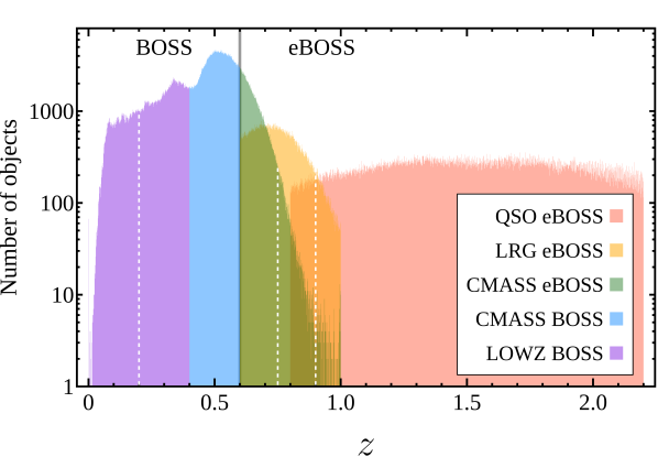
Figure 2: Redshift distribution of SDSS data used. The bin size adopted is $\Delta z=0.001$, the same used in the estimator. Dashed lines indicate data constraints. From left to right, the first dashed line marks the lower bound, $z>0.2$, due to the lack of mocks below this value. The second dashed line indicates the upper bound for CMASS eBOSS data, $z<0.75$, implemented to prevent estimator misbehavior with sparsely populated bins. Similarly, for LRG data, we adopt $z<0.9$, denoted by the third dashed line.

To infer the errors and biases of the estimator for eBOSS data, we used the 1000 EZmock realistic samples^{34, 35}, which include effects of clustering, survey geometry, redshift evolution, sample selection biases, and all systematic effects. These samples were modified to incorporate the Doppler effect by applying Eq. (1). For the BOSS catalogs, we applied the same approach using 1000 MultiDark-Patchy mocks³⁶. Both mock pipelines have been employed by the SDSS collaboration for comprehensive analysis of baryon acoustic oscillations and redshift space distortions^{37, 38, 39}.

The Emission Line Galaxy (ELG) eBOSS catalog was not considered as it covers merely $\sim 3\%$ of the sky. Given our aim to assess the largest scale modulation, the extent of sky coverage is crucial; hence, incorporating the ELG catalog yields negligible enhancement to our analysis. LOWZ objects with $z<0.2$ were not considered due to the lack of MultiDark-Patchy mocks for this redshift interval. Furthermore, CMASS eBOSS objects with $z>0.75$ were excluded, leading to a 4.6% reduction in the original catalog, and LRG eBOSS objects with $z>0.9$ were also omitted, accounting for a 6.6% reduction. These minor exclusions were necessary to prevent estimator misbehavior, as the estimator’s minimization becomes unstable in sparsely populated redshift bins (we adopted thin bins of $\Delta z=0.001$, see Methods).

Measuring the dipolar modulation

Achieving an unbiased estimation of the dipole and a reliable assessment of its uncertainty presents a significant challenge, especially when targeting a subtle signal of $\Delta_{1}\sim 10^{-3}$. To tackle this issue, we introduce a novel dipole estimator, implement a comprehensive bias-removal pipeline, and quantify uncertainty using state-of-the-art SDSS mock catalogs. The key elements of our measurement technique are outlined below, with details available in the Methods section. Our dipole estimator performs a tomographic least squares fit of the Doppler modulation around the de-Dopplered redshift monopole – the rest-frame monopole recalculated to remove the expected Doppler effect – for each redshift bin of $\Delta z=0.001$, and separately for each galactic cap (NGC and SGC).

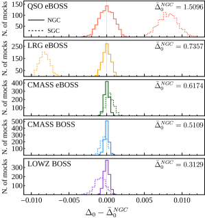
Figure 3: Distribution of monopoles ($\Delta_{0}$, average redshift) for the North (NGC) and South (SGC) Galactic Caps mocks. $\bar{\Delta}^{\rm NGC}_{0}$ represents the average NGC monopole. It is clear that the hemispheres have different depths.

First, separate analysis of the two galactic caps is essential for minimizing bias due to the differences between the NGC and SGC. Despite both caps being designed with equivalent equipment, analytical techniques, and observational strategies, a detailed examination of mocks and observational data reveal distinct depth variations between the hemispheres. As a result, the redshift monopoles $\Delta_{0}$ (average redshift considering the systematic weights) differ, as demonstrated in Fig. 3. These variations are comparable to, or exceed, the magnitude of the expected dipole $\Delta_{1}$ ($\sim 10^{-3}$). Given that the dipole is evaluated as a modulation around the monopole, acknowledging these discrepancies is essential to prevent bias in the combined estimation from the NGC and SGC datasets. Indeed, measuring the dipole, with and without hemisphere division, shows a typical deviation around $600$km/s for individual catalogs. When analyzing the two galactic caps together, the Doppler modulation is adjusted around the combined monopole of both hemispheres, with differences of the same order or bigger than the $\Delta_{1}c$ value of $\sim$370 km/s, expected within the $\Lambda$CDM model. Accounting for this effect is crucial for an accurate measurement.

The second key point regards the estimation of the monopole itself. In a full-sky survey the monopole and de-Dopplered monopole are expected to be the same, as the Doppler modulation increases the redshifts in one direction by the same factor that decreases in the opposite direction. However, for any sky-limited survey this antipodal symmetry is broken, and one has to use the de-Dopplered monopole, that is, the original rest-frame monopole, in order to prevent the introduction of bias. Accordingly, our estimator considers objects individually, with their respective systematic weights, comparing the observed and expected boosted redshift for its coordinates, given the de-Dopplered monopole of the very narrow redshift bin and the velocity being tested. The final result is obtained by minimizing across all bins and hemispheres simultaneously.

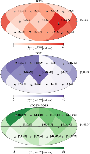
Figure 4: Bias maps in Mollweide projection. For each direction $i$, arrows originate from the fiducial expected values $\boldsymbol{\Delta}^{\rm{fid,i}}_{1}$, defined at the center of the pixels in the HEALPix $N_{\rm side}=1$ scheme, and point towards the direction of the average estimated vector from simulations $\boldsymbol{\Delta}^{\rm{sim,i}}_{1}$. Grey arrows depict the de-biased results, whereas black arrows represent the biased outcomes. The numbers indicate the difference vector between the de-biased results and the fiducials, with colors denoting the absolute value of this vector, all expressed in km/s.

Survey systematics, including observational strategies, footprint inhomogeneities, and variations in sky and telescope conditions, could introduce measurement bias. To assess and then adjust for this bias, we developed a series of mock catalogs from eBOSS’s EZmock sample and BOSS’s MultiDark-Patchy mocks. Notably, we utilized the realistic version of EZmock, which incorporates observational systematics, unlike the MultiDark-Patchy mocks that lack this aspect. Therefore, the findings related to the BOSS catalogs might be influenced by observational systematics. Our collection of mock catalogs was created by Doppler boosting 100 randomly selected mocks from both the eBOSS and BOSS surveys in 12 different directions, uniformly distributed across the sky. This process, utilizing a velocity of 370 km/s consistent with the kinematic interpretation of the CMB dipole, produced a total of 1200 mock catalogs for each tracer, summing up to 6000 mock catalogs overall.

Although we detected a relatively minor bias, we proceeded to apply a bias correction technique utilizing bi-linear interpolation of the bias vector. By subtracting the anticipated bias vector from the observed dipole measurement, we derived the de-biased value. This correction method was applied across both individual tracers and their combinations, as detailed in Methods. Fig. 4 demonstrates this process for the combined cases, by contrasting the average biased and de-biased dipole vectors against the benchmark dipole set in the simulations. See Extended Data Fig. 2 for the individual tracers’ cases. The corrected bias for each Cartesian component agrees with the benchmark values. This agreement was verified by comparing the mean difference vectors to the standard errors derived from 100 mocks per direction. Furthermore, we validated the estimator’s efficacy on the original 5000 mocks without Doppler effect, achieving the predicted outcomes after employing the bias correction, as illustrated in Extended Data Fig. 4.

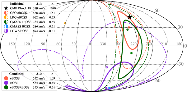
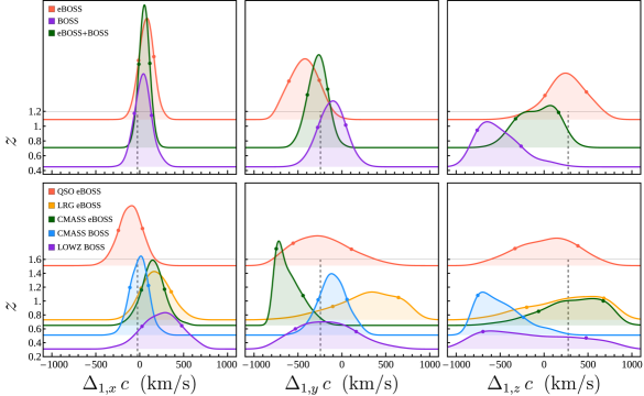
Figure 5: Final dipole measurements. (a) Mollweide projection displaying the dipole measurements in galactic coordinates, with contours representing the $1\sigma$ and $2\sigma$ confidence regions for combined measurements. The star symbol denotes the position of the CMB dipole for reference. (b) Probability distribution ridgeline plots in Cartesian coordinates, with dashed lines marking the CMB dipole values and dots indicating the $1\sigma$ confidence intervals.

When observed within the same redshift range, different tracers are expected to exhibit a similar clustering dipole, $\boldsymbol{\Delta_{1,\rm{int}}}$, which could lead to correlations between measurements not accounted for by our estimator. Despite our theoretical assessment indicating that the intrinsic dipole’s influence is minor (less than 2% of the anticipated dipole), we utilized the BOSS and eBOSS mock datasets to evaluate this effect through an alternative approach. Our empirical results reaffirm the theoretical prediction, establishing that the clustering dipole’s effect is indeed negligible, as depicted in Extended Data Fig. 3.

To accurately estimate the uncertainty associated with the dipole estimation, we applied a Doppler boost to the 1000 BOSS and eBOSS mock catalogs based on the best-fit model derived from the real dataset (for a total of 5000 mocks). We then processed these boosted mocks through the complete pipeline, effectively sampling the measurement distribution to determine the confidence intervals. Notably, the distributions obtained are consistent with the unbiased best-fit dipoles, serving as a further critical consistency check of the effectiveness of our bias removal technique across various dipole amplitudes, demonstrating that the bias correction is not significantly influenced by the absolute value of the dipole, including those different from the CMB-derived expectation used to create the bias maps.

Finally, given our utilization of a finite set (1000) of mock catalogs for statistical analysis, we ensure the robustness of our findings by employing two complementary methods, both leading to similar conclusions: a non-parametric Kernel Density Estimation (KDE) with a Gaussian kernel and a parametric best-fit distribution analysis using the Distfit Python module⁴⁰. This approach was consistent across error estimation and the determination of two-tailed significance regarding potential discrepancies with the CMB dipole. Our primary analysis leverages KDE. In agreement with our frequentist methodology for assessing uncertainties using mock catalogs, central values and $1\sigma$ uncertainties are determined using quantiles: the 50th percentile for the central value, and the 16th and 84th percentiles for the lower and upper uncertainty bounds, respectively.

Results and Discussion

Table 1: Dipole measurements with $1\sigma$ uncertainties and significance of tension against the CMB dipole.

					Dipole $\boldsymbol{\Delta}_{1}$				Significance of tension
	Case		$z$		$|\boldsymbol{v}|$ (km/s)	$l(^{\circ})$	$b(^{\circ})$		KDE	Distfit
	CMB		1090		$369.8^{+0.1}_{-0.1}$	$264.02^{+0.01}_{-0.01}$	$48.253^{+0.005}_{-0.005}$		–	–
	eBOSS		1.09		$552^{+169}_{-167}$	$280^{+12}_{-12}$	$30^{+15}_{-27}$		0.8$\sigma$	0.8$\sigma$
Combined	BOSS		0.45		$584^{+180}_{-243}$	$286^{+25}_{-146}$	$-77^{+52}_{-4}$		2.1$\sigma$	1.9$\sigma$
	eBOSS+BOSS		0.71		$353^{+123}_{-111}$	$281^{+14}_{-14}$	$-11^{+39}_{-30}$		1.4$\sigma$	1.3$\sigma$
	QSO eBOSS		1.51		$488^{+207}_{-187}$	$245^{+30}_{-89}$	$7^{+33}_{-44}$		0.2$\sigma$	0.2$\sigma$
Individual	LRG eBOSS		0.73		$662^{+200}_{-240}$	$60^{+232}_{-22}$	$37^{+14}_{-58}$		1.0$\sigma$	1.0$\sigma$
	CMASS eBOSS		0.65		$784^{+150}_{-160}$	$285^{+10}_{-13}$	$26^{+18}_{-33}$		1.6$\sigma$	1.2$\sigma$
	CMASS BOSS		0.51		$586^{+196}_{-251}$	$269^{+34}_{-143}$	$-78^{+62}_{-4}$		2.1$\sigma$	1.6$\sigma$
	LOWZ BOSS		0.31		$694^{+198}_{-247}$	$327^{+6}_{-284}$	$-35^{+73}_{-16}$		0.6$\sigma$	0.6$\sigma$

To evaluate the two-tailed significance, we compare the dipoles to the CMB value in Cartesian coordinates using two methods: a non-parametric Kernel Density Estimation (KDE) with a Gaussian kernel and a parametric best-fit distribution analysis conducted using the Distfit Python module⁴⁰. The table additionally lists the effective redshift for each scenario. For BOSS and eBOSS data, this corresponds to the weighted average redshift, which is equivalent to the monopole.

The analysis pipeline used in this study, including the evaluation of potential tension with the CMB dipole, was exclusively developed and validated using mock catalogs, ensuring that real data remained unexamined until after the methodology was established. Maintaining data blinding is critical to avoid reliance on a posteriori statistics, which might inadvertently skew the findings. In total, we processed 16000 mock catalogs, each subdivided into thousands of finely segmented redshift bins. The computational demand of this extensive study amounted to approximately 200000 CPU hours. For a visual representation of the data analysis pipeline, please refer to Extended Data Fig. 5.

Our findings are depicted in Fig. 5 and detailed in Table 1. The confidence contours illustrated in Fig. 5a were generated with the ligo.skymap Python module, a tool frequently utilized in the analysis of gravitational wave observations. Fig. 5b showcases the probability distributions ascertained through KDE. Table 1 lists the confidence intervals for both the magnitude and galactic coordinates of the velocities determined using the various catalogs and their combinations, alongside the significance of discrepancies relative to the CMB dipole. These significances were calculated for each Cartesian component and combined employing Fisher’s method⁴¹, see Methods.

Redshift dipole measurements indicate agreement with the CMB dipole, exhibiting a tension of $0.8\sigma$ for eBOSS data ($0.6<z<2.2$), $2.1\sigma$ for BOSS data ($0.2<z<0.6$), and $1.4\sigma$ for combined eBOSS+BOSS data ($0.2<z<2.2$). The most notable, albeit moderate, tension with the anticipated dipole arises from BOSS data within the redshift range $0.2<z<0.6$, where our findings suggest a deviation towards the southern hemisphere, despite the dipole’s magnitude closely matching expectations. This discrepancy slightly amplifies the overall tension between the combined measurement and the CMB dipole, while also decreasing the dipole magnitude due to the lower latitude of BOSS’s measured dipole. As previously highlighted, the BOSS mock catalogs did not incorporate realistic systematic effects, rendering the bias removal method unable to account for these unmodeled systematics, though they do incorporate veto weights to flag areas potentially affected by systematics. This consideration is relevant when evaluating the combined results’ overall increased tension and reduced dipole magnitude. However, it’s important to highlight that the bias correction applied across all scenarios resulted in only minor adjustments to the observed dipoles, revealing no significant evidence of systematic effects within the eBOSS or BOSS datasets.

Recent dipole estimations from number counts of radio galaxies and quasars have reported significantly higher dipole magnitudes as compared to CMB expectations, as illustrated in Fig. 1. Specifically, ref. 14 reported a velocity of $750\pm 81$ km/s, and ref. 15 reported $1131\pm 156$ km/s, both indicating about 5$\sigma$ tension with the CMB estimate. We compare our dipole measurements in Cartesian coordinates to these previous findings in Extended Data Fig. 6. Our analyses of eBOSS, BOSS, and eBOSS+BOSS data exhibit tensions in the 2-3$\sigma$ range when compared to these prior results, as detailed in Extended Data Table 1, suggesting that the possibility of a cosmological principle violation remains open.

Our analysis reveals that our motion with respect to distant galaxies and quasars is in close agreement with that suggested by the CMB dipole, as illustrated in Fig. 5 in both Galactic and Cartesian coordinates. This concordance implies that matter at cosmological distances of 1–5 Gpc shares the same rest frame as the CMB, located approximately 14 Gpc away, offering substantial support to the cosmological principle, which advocates for large-scale homogeneity and isotropy. However, significant tensions highlighted by previous studies suggest that the possibility of deviations from the cosmological principle cannot be fully excluded by our measurements alone. Progress in this area will require careful consideration of potential overlooked systematic factors in analyses based on number counts and redshifts, such as redshift evolution modeling, biases in estimators, or underestimation of uncertainties^{42, 43, 44, 45, 46}. Furthermore, validating the analysis pipeline using realistic mock catalogs and conducting blind data analyses, as undertaken in this study, remains critical.

Cosmology aims to comprehend the universe at its broadest spatial and temporal scales, relying on foundational principles to simplify our understanding of spacetime. Central to modern cosmology is the assumption of the universe’s statistical homogeneity and isotropy at large scales. The assumption’s validity stems from the observed near-isotropy of the universe and the Copernican principle, positing no special vantage point for observers: if all observers perceive the universe as isotropic, it must also be homogeneous. Our study tackles, therefore, a fundamental question on our place in the universe, reinforcing the mathematical and philosophical foundations of our standard cosmological model.

Methods

Estimator

We employ a least squares estimator to measure the dipole $\boldsymbol{\Delta}_{1}$ for each bin, based on the peculiar velocity hypothesis $\boldsymbol{\Delta}_{1}=-\boldsymbol{\beta}$. This calculation involves comparing the observed redshift distribution to the expected one for a theoretically isotropic $z$-field, boosted as per Eq. (1):

$$\chi^{2}_{\rm bin}(\boldsymbol{\Delta}_{1})=\frac{\sum_{i}^{N}w_{i}^{2}\left[z_{i}-\Delta^{dD}_{0,{\rm bin}}\delta(-\boldsymbol{\Delta}_{1},\boldsymbol{\hat{n}}^{\prime}_{i})\right]^{2}}{\sum_{i}^{N}w_{i}^{2}},$$ (6)

where $z_{i}$ is the observed redshift of object $i$ in a specific bin, $\boldsymbol{\hat{n}}^{\prime}_{i}$ is the observed redshift direction, $N$ denotes the total number of objects, and $w_{i}$ are the weights for each catalog (eBOSS and BOSS) defined as:

$$w_{i,\mathrm{eBOSS}} =w_{i,\mathrm{sys}}\cdot w_{i,\mathrm{noz}}\cdot w_{i,\mathrm{fc}}\,,$$ (7)

$$w_{i,\mathrm{BOSS}} =w_{i,\mathrm{sys}}\cdot(w_{i,\mathrm{noz}}+w_{i,\mathrm{fc}}-1)\,,$$ (8)

accounting for redshift failures ($w_{i,\mathrm{noz}}$), fiber collisions ($w_{i,\mathrm{fc}}$), and imaging systematics ($w_{i,\mathrm{sys}}$). Unlike other estimators, we consider the modulation around the “de-Dopplered” monopole $\Delta^{dD}_{0,{\rm bin}}$ of the respective bin, which is the average $z$ with the Doppler modulation removed:

$$\Delta^{dD}_{0,{\rm bin}}=\sum_{i}^{N}w_{i}z_{i}\delta(-\boldsymbol{\Delta}_{1},\boldsymbol{\hat{n}}^{\prime}_{i})^{-1}\bigg{/}\sum_{i}^{N}w_{i}\,.$$ (9)

Spectroscopic redshift measurement errors are negligible⁴⁷ and thus not considered. As discussed in Data, it’s necessary to analyze objects in the Northern and Southern Galactic Caps (NGC and SGC) separately due to distinct monopoles. Therefore, to find the complete sample’s best-fit dipole $\boldsymbol{\Delta}_{1}$, we minimize across all bins according to:

$$\chi^{2}(\boldsymbol{\Delta}_{\rm 1})=\sum_{\rm bin}\chi^{2}_{\rm bin,NGC}(\boldsymbol{\Delta}_{1})+\sum_{\rm bin}\chi^{2}_{\rm bin,SGC}(\boldsymbol{\Delta}_{1})\,.$$ (10)

We also note that in our analysis, we disregard terms of the order $\mathcal{O}(\beta^{2})$.

Data combination

To combine the results relative to the individual tracers and obtain the eBOSS, BOSS and eBOSS+BOSS results, we implemented the following steps: i) We determined the probability distributions $\{P^{\rm case}_{x},P^{\rm case}_{y},P^{\rm case}_{z}\}$ for each Cartesian component of the dipole vector $\{\Delta^{\rm case}_{1,x},\Delta^{\rm case}_{1,y},\Delta^{\rm case}_{1,z}\}$, across all individual cases; ii) We then multiplied the distributions of the Cartesian components together, followed by renormalization. For instance, prior to renormalization,

$$\!\!\!\!\!P^{\text{\tiny{BOSS}}}_{x}\! =\!P^{\text{\tiny{CMASS BOSS}}}_{x}\!\times\!P^{\text{\tiny{LOWZ BOSS}}}_{x}\,$$

$$P^{\text{\tiny{eBOSS}}}_{x}\! =\!P^{\text{\tiny{QSO eBOSS}}}_{x}\!\times\!P^{\text{\tiny{LRG eBOSS}}}_{x}\!\times\!P^{\text{\tiny{CMASS eBOSS}}}_{x}$$

$$P^{\text{\tiny{eBOSS+BOSS}}}_{x}\! =\!P^{\text{\tiny{eBOSS}}}_{x}\!\times\!P^{\text{\tiny{BOSS}}}_{x}\,,$$ (11)

for combining the distributions of the $x$ component; iii) Utilizing the combined distributions, we sampled 10000 vectors for the subsequent analysis.

Fisher’s method

Fisher’s method is utilized to consolidate results from multiple independent tests that assess the same hypothesis⁴¹. It aggregates the $p$-values from each test into a single test statistic, $X^{2}_{2k}$, through the equation:

$$X^{2}_{2k}=-2\sum_{i=1}^{k}\ln p_{i},$$ (12)

where $p_{i}$ represents the $p$-value for the $i$-th hypothesis test. Assuming the null hypothesis is valid and the $p_{i}$ values (or their corresponding test statistics) are independent, $X^{2}_{2k}$ follows a chi-squared distribution with $2k$ degrees of freedom, $k$ being the count of tests being combined. This can be used to determine the combined $p$-value, which we express in $\sigma$ units.

Correlations

Here, we used the BOSS and eBOSS mock datasets to assess whether different tracers display a comparable clustering dipole, attributable to their sampling of the same underlying dark matter density and velocity field. This effect potentially induces correlations between measurements. EZmock and MultiDark-Patchy individual tracers’ mocks, sharing identical ID numbers, originate from the same dark matter realization, ensuring they exhibit a similar clustering dipole within the same redshift range. We evaluated the dipole for each simulation, confirming that the measurements agree with an expected null dipole, as depicted in Extended Data Fig. 4. Based on these results, we calculated the correlation between different catalogs, finding that, as illustrated in Extended Data Fig. 3, the correlation is insignificant. This implies that the primary source of uncertainty is attributed to the finite tracers’ number density.

Bias removal

To construct the bias map, we Doppler boosted 100 mocks randomly chosen from both the eBOSS and BOSS surveys across 12 distinct directions, located at the pixel centers in the HEALPix $N_{\rm side}=1$ scheme, as illustrated in Fig. 4. HEALPix^{48, 49}, or Hierarchical Equal Area isoLatitude Pixelization, serves as an efficient system for handling spherical data, extensively employed in astrophysics and cosmology for pixelating the celestial sphere to streamline the analysis and visualization of astronomical datasets. This step assumes a velocity of 370 km/s, in line with the kinematic interpretation of the CMB dipole, yet, as noted in the main text, the bias map remains reliable across various dipole magnitudes, including the null case.

To compute the bias vector, we first estimate the dipole for each of the 100 simulations per direction (1200 simulations per tracer). We then derive the average difference vectors by subtracting the fiducial dipole vector $\boldsymbol{\Delta}^{\rm{fid,i}}_{1}$ for direction $i$ from the simulations’ average dipole vector $\langle\boldsymbol{\Delta}^{\rm{sim,i}}_{1}\rangle$. These average difference vectors, through their Cartesian components, establish the pixel values of the three bias maps for each tracer. Subsequent bi-linear interpolation of these bias maps for all Cartesian components is conducted using the get_interp_val function from the healpy Python module⁴⁹. Through this interpolation, we can de-bias the measured dipole, ensuring accurate analysis and interpretation of our findings.

BOSS mocks, while similar to EZmocks, do not incorporate systematic effects. As a result, the weights applied in the estimation of the bias maps are defined as follows:

$$w^{\rm{mocks}}_{i,\mathrm{BOSS}}=w_{i,\mathrm{veto}}\cdot w_{i,\mathrm{fc}},$$ (13)

where $w_{i,\mathrm{veto}}$ acts as a flag, being set to 1 for objects within the “veto mask” and 0 for those outside. The veto mask is employed to exclude sections of the sky that fail to adhere to specific quality standards, thus mitigating areas heavily influenced by systematics. Such standards may encompass regions lacking adequate observational coverage, areas subject to contamination, or any other conditions potentially compromising data quality.

The described method outlines the process for generating bias maps for individual tracers. To construct bias maps for the aggregate analyses of eBOSS, BOSS, and eBOSS+BOSS, we adopt the strategy used for combining data, as depicted in Eq. (11). Initially, we correct the 100 mock dipole measurements per direction using the bias maps specific to each tracer, then we aggregate these distributions and compare the composite average dipole to the fiducial one. The resultant difference vector forms the basis of the bias map for the combined analysis, which we subsequently interpolate to correct the measured dipoles derived from data combinations.

Data availability

All data is available starting from data.sdss.org/sas. The SDSS DR16 data used to perform the eBOSS measurements is available at dr17/eboss/lss/catalogs/DR16, and their respective EZmock catalogs at dr17/eboss/lss/EZmocks/v1_0_0/realistic. The SDSS DR12 BOSS data is accessible at dr12/boss/lss, and their respective MultiDark-Patchy mocks at dr12/boss/lss/dr12_multidark_patchy_mocks.

Code availability

The python code of the estimator and mock generation is hosted at github.com/pdsferreira/tomographic-redshift-dipole.

Author contributions

PSF and VM conceptualized the study and devised the methodology. PSF was responsible for coding and conducting the data analysis. Both PSF and VM collaboratively authored the manuscript.

Competing interests

The authors declare no competing interests.

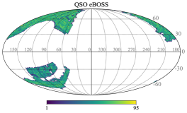
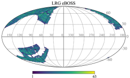
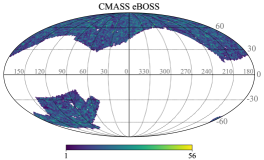
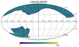
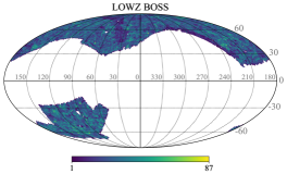
Figure Extended Data Fig. 1: Tracer distribution footprints. Number count maps for each tracer, presented in Mollweide projection using the HEALPix format with $N_{\rm side}=64$.

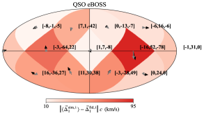
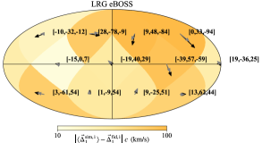
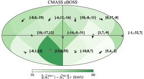
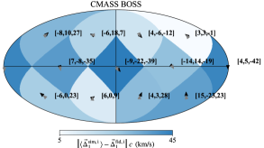
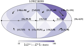
Figure Extended Data Fig. 2: Bias maps in Mollweide projection. Similar to Fig. 4 for the individual cases.

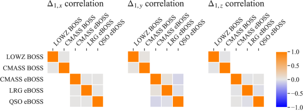
Figure Extended Data Fig. 3: Pearson correlation matrix between $\Delta_{1}$ measurements of different tracers. The correlations were obtained using the BOSS and eBOSS mocks. Correlations between the BOSS and eBOSS measurements are absent because their mocks were obtained independently.

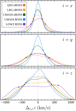
Figure Extended Data Fig. 4: Probability distributions of de-biased results without boost. The points mark the $1\sigma$ confidence intervals.

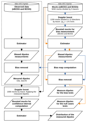
Figure Extended Data Fig. 5: Complete pipeline used in this work. The dashed region represents the steps using observed data. Orange lines indicate the steps of the null case tests (without boost). Blue lines indicate the steps of the bias measurement.

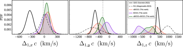
Figure Extended Data Fig. 6: Comparison of dipole measurements in Cartesian coordinates with previous estimates. The distributions for eBOSS, BOSS, eBOSS+BOSS analyses correspond to those presented in Fig. 5.

Table Extended Data Table 1: Significance of tension of previous estimations against our results.

	Dipole $\boldsymbol{\Delta}_{1}$			Significance of tension with
Measurement	$|\boldsymbol{v}|$ (km/s)	$l(^{\circ})$	$b(^{\circ})$	eBOSS	BOSS	eBOSS+BOSS
QSO (Secrest+2022)14	$750\pm 81$	$238\pm 7$	$31\pm 5$	2.7$\sigma$	2.1$\sigma$	2.3$\sigma$
RG (Wagenveld+2023)15	$1131\pm 156$	$270\pm 10$	$56\pm 17$	2.7$\sigma$	2.0$\sigma$	2.3$\sigma$

References

- [1] Planck Collaboration, Planck Collaboration I, “Planck 2018 results. I. Overview and the cosmological legacy of Planck,” Astron. Astrophys. 641 (2020) A1, arXiv:1807.06205 [astro-ph.CO].
- [2] E. R. Peterson et al., “The Pantheon+ Analysis: Evaluating Peculiar Velocity Corrections in Cosmological Analyses with Nearby Type Ia Supernovae,” Astrophys. J. 938 no. 2, (2022) 112, arXiv:2110.03487 [astro-ph.CO].
- [3] M. Scrimgeour et al., “The WiggleZ Dark Energy Survey: the transition to large-scale cosmic homogeneity,” Mon. Not. Roy. Astron. Soc. 425 (2012) 116–134, arXiv:1205.6812 [astro-ph.CO].
- [4] P. Ntelis et al., “Exploring cosmic homogeneity with the BOSS DR12 galaxy sample,” JCAP 06 (2017) 019, arXiv:1702.02159 [astro-ph.CO].
- [5] G. F. R. Ellis and J. E. Baldwin, “On the expected anisotropy of radio source counts,” MNRAS 206 (Jan., 1984) 377–381.
- [6] M. Plionis and I. Georgantopoulos, “The rosat x-ray background dipole,” Mon. Not. Roy. Astron. Soc. 306 (1999) 112, arXiv:astro-ph/9812391.
- [7] C. Blake and J. Wall, “Detection of the velocity dipole in the radio galaxies of the nrao vla sky survey,” Nature 416 (2002) 150–152, arXiv:astro-ph/0203385.
- [8] A. K. Singal, “Large Peculiar Motion of the Solar System from the Dipole Anisotropy in Sky Brightness due to Distant Radio Sources,” ApJ 742 no. 2, (Dec., 2011) L23, arXiv:1110.6260 [astro-ph.CO].
- [9] M. Rubart and D. J. Schwarz, “Cosmic radio dipole from NVSS and WENSS,” Astron. Astrophys. 555 (2013) A117, arXiv:1301.5559 [astro-ph.CO].
- [10] J. Colin, R. Mohayaee, M. Rameez, and S. Sarkar, “High redshift radio galaxies and divergence from the CMB dipole,” Mon. Not. Roy. Astron. Soc. 471 no. 1, (2017) 1045–1055, arXiv:1703.09376 [astro-ph.CO].
- [11] C. A. P. Bengaly, R. Maartens, and M. G. Santos, “Probing the Cosmological Principle in the counts of radio galaxies at different frequencies,” JCAP 04 (2018) 031, arXiv:1710.08804 [astro-ph.CO].
- [12] C. Murray, “The effects of lensing by local structures on the dipole of radio source counts,” Mon. Not. Roy. Astron. Soc. 510 no. 2, (2022) 3098–3101, arXiv:2112.06689 [astro-ph.CO].
- [13] J. Darling, “The Universe is Brighter in the Direction of Our Motion: Galaxy Counts and Fluxes are Consistent with the CMB Dipole,” Astrophys. J. Lett. 931 no. 2, (2022) L14, arXiv:2205.06880 [astro-ph.CO].
- [14] N. J. Secrest, S. von Hausegger, M. Rameez, R. Mohayaee, and S. Sarkar, “A Challenge to the Standard Cosmological Model,” Astrophys. J. Lett. 937 no. 2, (2022) L31, arXiv:2206.05624 [astro-ph.CO].
- [15] J. D. Wagenveld, H.-R. Klöckner, and D. J. Schwarz, “The cosmic radio dipole: Bayesian estimators on new and old radio surveys,” Astron. Astrophys. 675 (2023) A72, arXiv:2305.15335 [astro-ph.CO].
- [16] N. J. Secrest, S. von Hausegger, M. Rameez, R. Mohayaee, S. Sarkar, and J. Colin, “A Test of the Cosmological Principle with Quasars,” Astrophys. J. Lett. 908 no. 2, (2021) L51, arXiv:2009.14826 [astro-ph.CO].
- [17] N. Horstmann, Y. Pietschke, and D. J. Schwarz, “Inference of the cosmic rest-frame from supernovae Ia,” Astron. Astrophys. 668 (2022) A34, arXiv:2111.03055 [astro-ph.CO].
- [18] F. Sorrenti, R. Durrer, and M. Kunz, “The dipole of the Pantheon+SH0ES data,” JCAP 11 (2023) 054, arXiv:2212.10328 [astro-ph.CO].
- [19] S. Mastrogiovanni, C. Bonvin, G. Cusin, and S. Foffa, “Detection and estimation of the cosmic dipole with the einstein telescope and cosmic explorer,” Mon. Not. Roy. Astron. Soc. 521 no. 1, (2023) 984–994, arXiv:2209.11658 [astro-ph.CO].
- [20] G. Tasinato, “Kinematic anisotropies and pulsar timing arrays,” Phys. Rev. D 108 no. 10, (2023) 103521, arXiv:2309.00403 [gr-qc].
- [21] P. da S. Ferreira and M. Quartin, “First Constraints on the Intrinsic CMB Dipole and Our Velocity with Doppler and Aberration,” Phys. Rev. Lett. 127 no. 10, (2021) 101301, arXiv:2011.08385 [astro-ph.CO].
- [22] O. Roldan, A. Notari, and M. Quartin, “Interpreting the CMB aberration and Doppler measurements: boost or intrinsic dipole?,” JCAP 1606 no. 06, (2016) 026, arXiv:1603.02664 [astro-ph.CO].
- [23] B. Paczynski and T. Piran, “A Dipole Moment of the Microwave Background as a Cosmological Effect,” ApJ 364 (Dec., 1990) 341.
- [24] M. S. Turner, “A Tilted Universe (and Other Remnants of the Preinflationary Universe),” Phys. Rev. D 44 (1991) 3737–3748.
- [25] G. Domènech, R. Mohayaee, S. P. Patil, and S. Sarkar, “Galaxy number-count dipole and superhorizon fluctuations,” JCAP 10 (2022) 019, arXiv:2207.01569 [astro-ph.CO].
- [26] D. Langlois, “Cosmic microwave background dipole induced by double inflation,” Phys. Rev. D 54 (1996) 2447–2450, arXiv:gr-qc/9606066.
- [27] P. da S. Ferreira and M. Quartin, “Disentangling Doppler modulation, aberration and the temperature dipole in the CMB,” Phys. Rev. D 104 no. 6, (2021) 063503, arXiv:2107.10846 [astro-ph.CO].
- [28] V. Mittal, O. T. Oayda, and G. F. Lewis, “The Cosmic Dipole in the Quaia Sample of Quasars: A Bayesian Analysis,” arXiv:2311.14938 [astro-ph.CO].
- [29] T. M. Siewert, M. Schmidt-Rubart, and D. J. Schwarz, “Cosmic radio dipole: Estimators and frequency dependence,” Astron. Astrophys. 653 (2021) A9, arXiv:2010.08366 [astro-ph.CO].
- [30] A. Merloni, P. Predehl, et al., “erosita science book: Mapping the structure of the energetic universe.” 2012.
- [31] T. Nadolny, R. Durrer, M. Kunz, and H. Padmanabhan, “A new way to test the Cosmological Principle: measuring our peculiar velocity and the large-scale anisotropy independently,” JCAP 11 (2021) 009, arXiv:2106.05284 [astro-ph.CO].
- [32] eBOSS Collaboration, A. J. Ross et al., “The Completed SDSS-IV extended Baryon Oscillation Spectroscopic Survey: Large-scale structure catalogues for cosmological analysis,” Mon. Not. Roy. Astron. Soc. 498 no. 2, (2020) 2354–2371, arXiv:2007.09000 [astro-ph.CO].
- [33] B. Reid et al., “SDSS-III Baryon Oscillation Spectroscopic Survey Data Release 12: galaxy target selection and large scale structure catalogues,” Mon. Not. Roy. Astron. Soc. 455 no. 2, (2016) 1553–1573, arXiv:1509.06529 [astro-ph.CO].
- [34] C.-H. Chuang, F.-S. Kitaura, F. Prada, C. Zhao, and G. Yepes, “EZmocks: extending the Zel’dovich approximation to generate mock galaxy catalogues with accurate clustering statistics,” Mon. Not. Roy. Astron. Soc. 446 (2015) 2621–2628, arXiv:1409.1124 [astro-ph.CO].
- [35] C. Zhao et al., “The completed SDSS-IV extended Baryon Oscillation Spectroscopic Survey: 1000 multi-tracer mock catalogues with redshift evolution and systematics for galaxies and quasars of the final data release,” Mon. Not. Roy. Astron. Soc. 503 no. 1, (2021) 1149–1173, arXiv:2007.08997 [astro-ph.CO].
- [36] F.-S. Kitaura et al., “The clustering of galaxies in the SDSS-III Baryon Oscillation Spectroscopic Survey: mock galaxy catalogues for the BOSS Final Data Release,” Mon. Not. Roy. Astron. Soc. 456 no. 4, (2016) 4156–4173, arXiv:1509.06400 [astro-ph.CO].
- [37] BOSS Collaboration, S. Alam et al., “The clustering of galaxies in the completed SDSS-III Baryon Oscillation Spectroscopic Survey: cosmological analysis of the DR12 galaxy sample,” Mon. Not. Roy. Astron. Soc. 470 no. 3, (2017) 2617–2652, arXiv:1607.03155 [astro-ph.CO].
- [38] eBOSS Collaboration, J. Hou et al., “The Completed SDSS-IV extended Baryon Oscillation Spectroscopic Survey: BAO and RSD measurements from anisotropic clustering analysis of the Quasar Sample in configuration space between redshift 0.8 and 2.2” Mon. Not. Roy. Astron. Soc. 500 no. 1, (2020) 1201–1221, arXiv:2007.08998 [astro-ph.CO].
- [39] eBOSS Collaboration, H. Gil-Marin et al., “The Completed SDSS-IV extended Baryon Oscillation Spectroscopic Survey: measurement of the BAO and growth rate of structure of the luminous red galaxy sample from the anisotropic power spectrum between redshifts 0.6 and 1.0” Mon. Not. Roy. Astron. Soc. 498 no. 2, (2020) 2492–2531, arXiv:2007.08994 [astro-ph.CO].
- [40] E. Taskesen, “distfit is a python library for probability density fitting.” 01, 2020. https://erdogant.github.io/distfit. If you use this software, please cite it using these metadata.
- [41] R. A. Fisher, Statistical Methods for Research Workers. Oliver and Boyd, Edinburgh, 12 ed., 1954.
- [42] C. Gibelyou and D. Huterer, “Dipoles in the Sky,” Mon. Not. Roy. Astron. Soc. 427 (2012) 1994–2021, arXiv:1205.6476 [astro-ph.CO].
- [43] C. Dalang and C. Bonvin, “On the kinematic cosmic dipole tension,” Mon. Not. Roy. Astron. Soc. 512 no. 3, (2022) 3895–3905, arXiv:2111.03616 [astro-ph.CO].
- [44] C. Guandalin, J. Piat, C. Clarkson, and R. Maartens, “Theoretical Systematics in Testing the Cosmological Principle with the Kinematic Quasar Dipole,” Astrophys. J. 953 no. 2, (2023) 144, arXiv:2212.04925 [astro-ph.CO].
- [45] L. Dam, G. F. Lewis, and B. J. Brewer, “Testing the cosmological principle with CatWISE quasars: a bayesian analysis of the number-count dipole,” Mon. Not. Roy. Astron. Soc. 525 no. 1, (2023) 231–245, arXiv:2212.07733 [astro-ph.CO].
- [46] P. J. E. Peebles, “Anomalies in physical cosmology,” Annals Phys. 447 (2022) 169159, arXiv:2208.05018 [astro-ph.CO].
- [47] A. S. Bolton, D. J. Schlegel, et al., “Spectral Classification and Redshift Measurement for the SDSS-III Baryon Oscillation Spectroscopic Survey,” AJ 144 no. 5, (Nov., 2012) 144, arXiv:1207.7326 [astro-ph.CO].
- [48] K. M. Górski, E. Hivon, A. J. Banday, B. D. Wandelt, F. K. Hansen, M. Reinecke, and M. Bartelmann, “HEALPix: A Framework for High-Resolution Discretization and Fast Analysis of Data Distributed on the Sphere,” ApJ 622 (Apr., 2005) 759–771, arXiv:astro-ph/0409513.
- [49] A. Zonca, L. Singer, D. Lenz, M. Reinecke, C. Rosset, E. Hivon, and K. Gorski, “healpy: equal area pixelization and spherical harmonics transforms for data on the sphere in python,” Journal of Open Source Software 4 no. 35, (Mar., 2019) 1298. https://doi.org/10.21105/joss.01298.
Acknowledgments
It is a pleasure to thank Nathan Secrest for useful comments and discussions. Funding: PSF thanks FAPES (Brazil) for financial support. VM thanks CNPq (Brazil) and FAPES (Brazil) for partial financial support. Sci-Com cluster: We acknowledge the use of the computational resources provided by the Sci-Com Lab of the Department of Physics at UFES, which was funded by FAPES. Joint CHE / Milliways cluster: We acknowledge the use of the computational resources of the joint CHE / Milliways cluster, supported by a FAPERJ grant E-26/210.130/2023. HOTCAT cluster: We acknowledge the use of the HOTCAT computing infrastructure of the Astronomical Observatory of Trieste of the National Institute for Astrophysics (INAF, Italy). MultiDark-Patchy mocks: The massive production of all MultiDark-Patchy mocks for the BOSS Final Data Release has been performed at the BSC Marenostrum supercomputer, the Hydra cluster at the Instituto de Fısica Teorica UAM/CSIC, and NERSC at the Lawrence Berkeley National Laboratory. We acknowledge support from the Spanish MICINNs Consolider-Ingenio 2010 Programme under grant MultiDark CSD2009-00064, MINECO Centro de Excelencia Severo Ochoa Programme under grant SEV- 2012-0249, and grant AYA2014-60641-C2-1-P. The MultiDark-Patchy mocks was an effort led from the IFT UAM-CSIC by F. Prada’s group (C.-H. Chuang, S. Rodriguez-Torres and C. Scoccola) in collaboration with C. Zhao (Tsinghua U.), F.-S. Kitaura (AIP), A. Klypin (NMSU), G. Yepes (UAM), and the BOSS galaxy clustering working group. EZmocks: We acknowledge the use of the EZmocks galaxy mock catalogues with redshift evolution and systematics for galaxies and quasars of the final SDSS-IV data release [35]. SDSS-III (BOSS) data: Funding for SDSS-III has been provided by the Alfred P. Sloan Foundation, the Participating Institutions, the National Science Foundation, and the U.S. Department of Energy Office of Science. The SDSS-III web site is http://www.sdss3.org/. SDSS-III is managed by the Astrophysical Research Consortium for the Participating Institutions of the SDSS-III Collaboration including the University of Arizona, the Brazilian Participation Group, Brookhaven National Laboratory, Carnegie Mellon University, University of Florida, the French Participation Group, the German Participation Group, Harvard University, the Instituto de Astrofisica de Canarias, the Michigan State/Notre Dame/JINA Participation Group, Johns Hopkins University, Lawrence Berkeley National Laboratory, Max Planck Institute for Astrophysics, Max Planck Institute for Extraterrestrial Physics, New Mexico State University, New York University, Ohio State University, Pennsylvania State University, University of Portsmouth, Princeton University, the Spanish Participation Group, University of Tokyo, University of Utah, Vanderbilt University, University of Virginia, University of Washington, and Yale University. SDSS-IV (eBOSS) data: Funding for the Sloan Digital Sky Survey IV has been provided by the Alfred P. Sloan Foundation, the U.S. Department of Energy Office of Science, and the Participating Institutions. SDSS acknowledges support and resources from the Center for High-Performance Computing at the University of Utah. The SDSS web site is www.sdss4.org. SDSS is managed by the Astrophysical Research Consortium for the Participating Institutions of the SDSS Collaboration including the Brazilian Participation Group, the Carnegie Institution for Science, Carnegie Mellon University, Center for Astrophysics | Harvard & Smithsonian (CfA), the Chilean Participation Group, the French Participation Group, Instituto de Astrofísica de Canarias, The Johns Hopkins University, Kavli Institute for the Physics and Mathematics of the Universe (IPMU) / University of Tokyo, the Korean Participation Group, Lawrence Berkeley National Laboratory, Leibniz Institut für Astrophysik Potsdam (AIP), Max-Planck-Institut für Astronomie (MPIA Heidelberg), Max-Planck-Institut für Astrophysik (MPA Garching), Max-Planck-Institut für Extraterrestrische Physik (MPE), National Astronomical Observatories of China, New Mexico State University, New York University, University of Notre Dame, Observatório Nacional / MCTI, The Ohio State University, Pennsylvania State University, Shanghai Astronomical Observatory, United Kingdom Participation Group, Universidad Nacional Autónoma de México, University of Arizona, University of Colorado Boulder, University of Oxford, University of Portsmouth, University of Utah, University of Virginia, University of Washington, University of Wisconsin, Vanderbilt University, and Yale University.