Visibility-Aware Keypoint Localization for 6DoF Object Pose Estimation

Abstract

Localizing predefined 3D keypoints in a 2D image is an effective way to establish 3D-2D correspondences for 6DoF object pose estimation. However, unreliable localization results of invisible keypoints degrade the quality of correspondences. In this paper, we address this issue by localizing the important keypoints in terms of visibility. Since keypoint visibility information is currently missing in dataset collection process, we propose an efficient way to generate binary visibility labels from available object-level annotations, for keypoints of both asymmetric objects and symmetric objects. We further derive real-valued visibility-aware importance from binary labels based on PageRank algorithm. Taking advantage of the flexibility of our visibility-aware importance, we construct VAPO (Visibility-Aware POse estimator) by integrating the visibility-aware importance with a state-of-the-art pose estimation algorithm, along with additional positional encoding. Extensive experiments are conducted on popular pose estimation benchmarks including Linemod, Linemod-Occlusion, and YCB-V. The results show that, VAPO improves both the keypoint correspondences and final estimated poses, and clearly achieves state-of-the-art performances.

1 Introduction

Figure 1: Motivation of our visibility-aware keypoint localization method. For the input image (a), we visualize visibility of predefined keypoints in (b). Each row shows internal visibility w.r.t. self-occlusion and each column shows external visibility w.r.t. occlusion. Without direct observations in the image, localizing invisible keypoints (the yellow ones) may be challenging and degrade the quality of 3D-2D correspondences. We propose to estimate visibility-aware importance for each keypoint, and discard keypoints with low importance.

Given a single input RGB image, instance-level 6DoF object pose estimator recovers rotation and translation of a rigid object with respect to a calibrated camera. The estimated pose information is crucial in many real-world applications, including robot manipulation [75, 61, 62], autonomous driving [35, 67, 29], augmented reality [36, 58], 3D reconstruction [37, 66], etc. To increase the robustness against various imaging conditions, the majority of the existing methods [46, 59, 39, 15, 44, 69, 42, 30, 51, 54, 31] first generate correspondences between 2D image pixels and 3D object points, and then regress the pose via any available Perspective-n-Point (PnP) solver [28, 64, 2].

Based on the correspondence estimation process, previous methods can be divided into two categories. The first kind of methods [69, 42, 30, 64, 7, 54] estimate corresponding 3D coordinate on the object surface for each 2D pixel, which can be treated as an image-to-image translation task. The other kind of methods [46, 59, 72, 44, 31] localize predefined 3D keypoints in the input image to obtain 3D-2D correspondences. Compared with image-to-image translation based methods, keypoint-based methods efficiently encode the object geometry information, which facilitates the pose estimation process. The pioneering keypoint-based works localize the eight corners of the 3D object bounding box [46, 59]. The follow-up works [72, 44] adopt sparse keypoints (e.g., 8 keypoints) sampled from the object surface. Recently, CheckerPose [31] is proposed to generate dense correspondences via localizing dense 3D keypoints and it achieves state-of-the-art performance for object pose estimation.

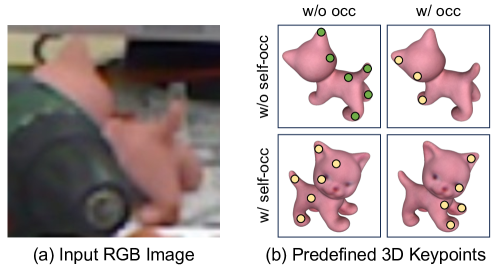
To obtain better correspondences for object pose estimation, a great amount of effort has been devoted to improve the localization precision of each keypoint. However, existing keypoint-based methods have a common issue illustrated in Fig. 1, that is, a large portion of predefined keypoints are invisible in the input image, due to occlusion or self-occlusion. Without direct observations, the localization results of such keypoints may be unreliable. Since the ultimate goal of keypoint localization is to establish reliable 3D-2D correspondences for 6DoF pose estimation, it may be unnecessary to localize each predefined keypoint.

To overcome the above issue, we propose to estimate visibility-aware importance for each keypoint, and discard unimportant keypoints before localization. As a starting point, we can represent keypoint visibility as a binary value. We notice that such information is manually annotated in datasets from other domains, e.g., human pose estimation [21, 1]. However, annotations of keypoint visibility are currently missing in 6DoF object pose datasets. To get rid of expensive manual annotation process, we propose an efficient way to generate visibility labels from available object-level annotations. We decompose visibility into two binary terms w.r.t. external occlusion and internal self-occlusion, respectively. The external visibility term can be obtained from available object segmentation masks. The internal visibility term can be determined based on surface normals and camera ray directions, inspired by back-face culling [26, 71] in rendering. For symmetric objects, we derive modified computation to ensure consistency.

Besides binary labels, we further derive real-valued measure to comprehensively reflect the visibility-aware importance of each keypoint. To do this, we create a $k$-nearest neighbor ($k$-NN) graph from the predefined keypoints, and measure the closeness of each keypoint to visible ones as importance. We utilize Personalized PageRank (PPR) [40] as our proximity measure, and derive an analytical formula of importance which can be efficiently evaluated.

Our visibility-aware importance can be easily integrated into existing keypoint-based 6DoF pose estimator to boost performance. We adopt CheckerPose [31] as our base framework, which utilizes graph neural networks (GNNs) to model the interactions among dense keypoints. While CheckerPose is originally designed to localize every keypoint in a predefined set, we add a visibility-aware importance predictor and eliminate half of the keypoints with low importance. We further enhance the keypoint embedding in GNNs with positional encoding, and use a two-stage training strategy to efficiently train the deep network.

To summarize, we make the following contributions:

• We propose to localize important keypoints in terms of visibility, to obtain high-quality 3D-2D correspondences for 6DoF object pose estimation.

• From object-level annotations, we derive an efficient way to generate binary keypoint visibility labels, for both asymmetric objects and symmetric ones.

• We further derive a concise analytic formula to produce real-valued visibility-aware keypoint importance based on Personalized PageRank.

• We demonstrate that our visibility-aware importance can be easily incorporated to existing keypoint-based method to boost performance.

We conduct extensive experiments on Linemod [11], Linemod-Occlusion [3], and YCB-V [68] to demonstrate the effectiveness of our method. We will release the source code of our work upon the publication.

2 Related Work

In this section, we review previous studies related to our work, including 6DoF pose estimation from RGB inputs and applications of visibility estimation.

Direct Methods. Traditionally, object poses are estimated by template matching with hand-crafted features [18, 9, 10], which can not work well on textureless objects. Features learned from neural networks are also investigated to directly produce the final estimated poses [68, 63, 53, 24, 55]. However, due to the nonlinearity of 3D rotations, direct methods are still unstable without predicting intermediate geometric representations, e.g., 3D-2D correspondences.

Image-to-image Translation Based Methods. One popular way to establish 3D-2D correspondences can be regarded as an image-to-image translation task [42]. Specifically, for each 2D pixel, the corresponding 3D point on the object surface is predicted in the object frame [42, 30, 64, 7]. The 3D coordinates can also be represented as UV-maps [69], local surface embeddings [45], hierarchical binary encodings [54], etc. The dense correspondences are robust against various imaging conditions, such as occlusions, background clutter, etc. With the correspondences, object pose can be recovered via existing PnP solvers [28, 2], coupled with RANSAC to remove outliers. Recent methods [64, 7, 33] also use neural networks to produce final poses from the correspondences.

Keypoint-based Methods. Localizing predefined keypoints in the input image is also widely used for constructing 3D-2D correspondences. For simplicity, previous works [46, 59, 15, 14, 16, 39] localize the 3D object bounding box corners. Other works [72, 44, 31] also adopt keypoints on the object surface obtained via farthest point sampling (FPS), which tend to achieve better performance since they are closely related to the object pixels. While existing methods mainly utilize sparse keypoints (e.g., 8 keypoints), CheckerPose [31] localizes dense keypoints (e.g., 512 keypoints) to construct dense 3D-2D correspondences, which increases the robustness similar to the image-to-image translation based methods. Though previous methods demonstrate the importance of predefining proper keypoints, no keypoint can always be visible in any input image.

Visibility Estimation for 3D Vision and Graphs. For an object in the 3D space, not all parts are visible in its 2D images. For rigid pose estimation, visibility can be used to select reliable correspondences [31, 17]. Still, each correspondence is generated despite its visibility. Differentiable surface visibility is developed to facilitate render-and-compare framework [49]. Visibility can also be efficiently estimated in online tracking with a known initial pose and smooth changes [27]. For nonrigid pose estimation, keypoint localization results are usually represented as heatmaps, and visibility can be implicitly interpreted from heatmaps [38, 13, 8]. Moreover, keypoint visibility is manually annotated in various datasets [21, 1, 32], and can be used as supervision signals [47, 74]. Beyond pose estimation, visibility determination also facilitates various tasks in computer vision and graphics. In rendering of large polygonal models, back-facing polygons are eliminated to speed up the rendering process [26, 71]. Visibility can also be utilized for mesh simplification [70], point cloud visualization [23, 22], novel view generation [50, 52, 56, 34, 20], multi-view aggregation [73, 6], etc.

Our work follows the keypoint-based framework for 6DoF pose estimation. We focus on keypoints with high visibility-aware importance, and effectively generate supervision signals from object-level annotations.

3 Method

Our work focuses on instance-level pose estimation for a rigid object $O$ with available CAD model. We sample 3D keypoints $\mathcal{P}$ from the CAD model, and estimate the importance of each keypoint $\mathbf{p}\in\mathcal{P}$ w.r.t. visibility in the input RGB image $I$. We then localize the subset of $\mathcal{P}$ with high importance, and obtain rotation $\mathbf{R}\in SO(3)$ and translation $\mathbf{t}\in\mathbb{R}^{3}$ from the localization results via a PnP solver [28, 2]. We describe our method, named VAPO, in details as follows.

3.1 Generating Visibility Labels from Object-Level Annotations

Keypoint-level annotations are typically unavailable in existing 6DoF object pose datasets, such as Linemod [11], Linemod-Occlusion [3], YCB-V [68], etc. While keypoint visibility labels are provided by datasets from other domains, e.g., Leeds Sports Poses [21], MPII Human Pose [1], COCO [32], etc., such labels require expensive human labelling efforts. Moreover, there is no canonical way to predefine keypoints for 6DoF pose. Even though one can manually annotate the visibility of a specific set of keypoints, missing label issue still arises when object pose estimator utilizes a different set of keypoints, e.g., denser keypoints.

To avoid expensive manual annotation and provide flexibility for different 3D keypoints $\mathcal{P}$, we instead seek an efficient way to generate visibility labels from available object-level annotation, i.e., rotation $\mathbf{R}$, translation $\mathbf{t}$, and object segmentation masks $M$. A keypoint $\mathbf{p}\in\mathcal{P}$ is visible if and only if it is free from both occlusions and self-occlusions. Thus we can decompose visibility into two binary terms: the external visibility $V_{\mathrm{ex}}(\mathbf{p})\in\{0,1\}$ w.r.t. occlusions from other objects, and the internal visibility $V_{\mathrm{in}}(\mathbf{p})\in\{0,1\}$ w.r.t. self-occlusions. The overall visibility $V(\mathbf{p})\in\{0,1\}$ can be computed by

$$V(\mathbf{p})=V_{\mathrm{ex}}(\mathbf{p})\times V_{\mathrm{in}}(\mathbf{p}),$$ (1)

and keypoint $\mathbf{p}$ satisfies $V(\mathbf{p})=1$ if and only if $V_{\mathrm{ex}}(\mathbf{p})=1$ and $V_{\mathrm{in}}(\mathbf{p})=1$.

Since visible segmentation mask $M_{\mathrm{vis}}$ of the object $O$ reflects occlusions from other objects, we can determine $V_{\mathrm{ex}}(\mathbf{p})$ by

$$V_{\mathrm{ex}}(\mathbf{p})=\begin{cases}1,&\text{if }\boldsymbol{\pi}(\mathbf{p};\mathbf{R},\mathbf{t})\in M_{\mathrm{vis}}\\ 0,&\text{otherwise}\end{cases},$$ (2)

where $\boldsymbol{\pi}(\mathbf{p};\mathbf{R},\mathbf{t})$ is the perspective projection of $\mathbf{p}$ using pose $(\mathbf{R},\mathbf{t})$.

To determine whether keypoint $\mathbf{p}\in\mathcal{P}$ is self-occluded, we can check whether the direction from $\mathbf{p}$ towards the camera has additional intersections with the object surface. However, it is time-consuming to check the intersections on the fly during training. Inspired by back-face culling [26, 71] in rendering, we compute $V_{\mathrm{in}}(\mathbf{p})$ by

$$V_{\mathrm{in}}(\mathbf{p})=\begin{cases}1,&\text{if }\mathbf{d_{p}}^{(c)}\cdot\mathbf{n}_{\mathbf{p}}^{(c)}>0\\ 0,&\text{otherwise}\end{cases},$$ (3)

where $\mathbf{d_{p}}^{(c)}$ denotes the direction from $\mathbf{p}$ towards the camera in the camera space, and $\mathbf{n}_{\mathbf{p}}^{(c)}$ denotes the surface normal at $\mathbf{p}$ in the camera space. In the camera space, the camera is placed at the origin $[0,0,0]^{\top}$, and then

$$\mathbf{d_{p}}^{(c)}=-\mathbf{p}^{(c)}=-(\mathbf{R}\mathbf{p}+\mathbf{t}),$$ (4)

where $\mathbf{p}^{(c)}$ is the keypoint coordinate in the camera space. With the 3D CAD model, we have access to the surface normal $\mathbf{n}_{\mathbf{p}}$ in the object frame, and we get

$$\mathbf{n}_{\mathbf{p}}^{(c)}=\mathbf{R}\mathbf{n}_{\mathbf{p}},$$ (5)

thus Eq. 3 can be efficiently computed from available object-level annotations.

For a convex object, $V_{\mathrm{in}}(\mathbf{p})=1$ is a necessary and sufficient condition for $\mathbf{p}$ being not self-occluded. For a non-convex object, $V_{\mathrm{in}}(\mathbf{p})=1$ is a necessary condition, and we use Eq. 3 for several reasons. Firstly, if $V_{\mathrm{in}}(\mathbf{p})=0$, then $\mathbf{p}$ must be self-occluded, and we can safely eliminate $\mathbf{p}$ or reduce the importance of $\mathbf{p}$ in localization process. Secondly, a non-convex object tends to have a complex shape, and we might obtain better understanding of the object by keeping a small portion of self-occluded keypoints. Thirdly, we can efficiently label $V_{\mathrm{in}}(\mathbf{p})$ using available object-level annotations, which significantly facilitates the training process.

3.2 Handling Visibility of Symmetric Objects

Figure 2: Illustration of selecting the proper pose for symmetric objects. In the camera space, the camera is placed at the origin $O$ and looks at the direction $y>0$. The visible points are highlighted in red. (a) The object is translated along $y$-axis by $\mathbf{t}$. (b) The object is rotated $27^{\circ}$ counterclockwise around its center and then translated by $\mathbf{t}$. (c) The object is rotated $27^{\circ}$ clockwise and then translated by $\mathbf{t}$, but the visible points are significantly different from (b). (d) The object is rotated by larger degrees to get equivalent appearance of (c), and the visible points are more consistent with (b).

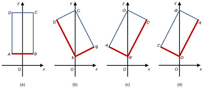
For a symmetric object, the input image corresponds to multiple equivalent poses w.r.t. the symmetry transformations $\mathcal{S}$. In practice, datasets usually provide only one annotated pose. From the perspective of keypoint visibility, however, it may not be optimal to directly use the annotated pose to generate visibility labels. Let us consider a 2D case without external occlusion for simplicity. As illustrated in Fig. 2 (a), the symmetry transformations $\mathcal{S}$ contain the identity matrix $\mathbf{I}$ and the one that rotates the object around the center for $180^{\circ}$. As shown in Fig. 2 (b), the annotated pose is a combination of a slight counterclockwise rotation around object center (denoted as $\mathbf{R}_{1}$) and a translation $\mathbf{t}$ along $y$-axis, and the corresponding visible points are on the edges $AB$ and $DA$. While in Fig. 2 (c), the annotated rotation is a slight clockwise rotation around center (denoted as $\mathbf{R}_{2}$), and the corresponding visible points appear on the edges $AB$ and $BC$. Since $|BC|=|DA|\gg|AB|$, the visible points corresponding to $(\mathbf{R}_{1},\mathbf{t})$ and $(\mathbf{R}_{2},\mathbf{t})$ are dramatically different. To make $V(\mathbf{p})$ in Fig. 2 (c) more consistent with Fig. 2 (b), we can modify the annotated pose to an equivalent one to make visible points appear on the edges $DA$ and $CD$, as shown in Fig. 2 (d).

To enforce the consistency of keypoint visibility labels, we can modify the annotated pose to maximize the number of internally visible keypoints in a fixed subset of keypoints $\mathcal{P}_{\mathrm{sym}}$. We consider internal visibility $V_{\mathrm{in}}$ because self-occlusion always exists and is not effected by external objects. For an object with discrete symmetry, before the whole training process, we obtain $\mathcal{P}_{\mathrm{sym}}$ by finding the largest visible subset under sampled poses. In practice, we uniformly sample 2,562 rotation matrices in $SO(3)$, and use a fixed translation $\mathbf{t}$ along the camera looking direction. Then during training, we can enumerate the finite equivalent poses to find the one maximizing internally visible keypoints in $\mathcal{P}_{\mathrm{sym}}$. For an object with continuous symmetry, we further derive an analytic solution. Without loss of generality, we assume $z$-axis is a symmetry axis. We modify the original annotated rotation matrix by right-multiplying rotation around $z$-axis $\mathbf{R}_{z}(\theta)$, where $\theta$ is the rotation angle around $z$-axis, and is determined by

$$\theta=\begin{cases}\pi/2+[b>0]\pi,&\text{if }a=0\\ \arctan{(b/a)}+[a>0]\pi,&\text{otherwise }\end{cases},$$ (6)

where $a,b$ are the first and second entry of $\mathbf{R}^{\top}\mathbf{t}$, respectively, $[\cdot]$ is Iverson bracket outputting binary values $\{0,1\}$. We provide more details including the derivation in the Supplementary Material.

3.3 Visibility-Aware Importance via Personalized PageRank

So far we have discussed how to assign binary labels for keypoint visibility. While visible points are clearly more useful than invisible ones for pose estimation, not all visible points are equally important, depending on the distribution of these points and the specific estimation algorithms. Moreover, if an invisible keypoint is close to visible ones, localizing it may not be difficult. To address these issues, we propose to compute real-valued visibility-aware importance by measuring the closeness to visible keypoints w.r.t. a specific measure of the proximity.

In practice, we adopt Personalized PageRank (PPR) as our proximity measure, which is a variation of PageRank [40] based on a random walk model. Specifically, we build a directed $k$-nearest neighbor ($k$-NN) graph $G$ from predefined keypoints $\mathcal{P}$. For each keypoint $\mathbf{p}$, we create edges from $\mathbf{p}$ to its $k$-nearest neighbors. We define transition matrix $\mathbf{T}$ as

$$\mathbf{T}=\frac{1}{k}\mathbf{A}^{\top},$$ (7)

where $\mathbf{A}$ is the adjacency matrix of $G$. With probability $c\in(0,1)$, a random walker on $G$ moves along edges following $\mathbf{T}^{\top}$. With probability $1-c$, the random walker restarts at any visible keypoint with uniform probability. $c$ is often called damping factor, and we assign $c$ the widely used value 0.85. We use the stationary probability distribution $\mathbf{r}$ over $N$ keypoints to measure closeness to visible keypoints, where each entry of $\mathbf{r}$ represents the probability that the random walker resides on the corresponding keypoint. We can obtain $\mathbf{r}$ by solving the following equation

$$\mathbf{r}=c\mathbf{T}\mathbf{r}+(1-c)\mathbf{s},$$ (8)

where $\mathbf{s}$ is the restart vector, and the entry of keypoint $\mathbf{p}$ is determined from binary visibility labels as

$$\mathbf{s}(\mathbf{p})=\begin{cases}1/N_{\mathrm{vis}},&\text{if }V(\mathbf{p})=1\\ 0,&\text{otherwise}\end{cases},$$ (9)

where $N_{\mathrm{vis}}$ denotes the number of visible keypoints. By rearranging Eq. 8, we can compute $\mathbf{r}$ as

$$\mathbf{r}=\mathbf{T}_{\mathrm{PPR}}\mathbf{s},$$ (10)

where

$$\mathbf{T}_{\mathrm{PPR}}\stackrel{{\scriptstyle\text{def}}}{{=}}(1-c)(\mathbf{I}-c\mathbf{T})^{-1}.$$ (11)

Note that $\mathbf{I}-c\mathbf{T}$ is invertible thus $\mathbf{T}_{\mathrm{PPR}}$ is well-defined in Eq. 11. Moreover, $\mathbf{T}_{\mathrm{PPR}}$ is invariant for the object, so we can precompute $\mathbf{T}_{\mathrm{PPR}}$ using Eq. 11 and store it, and then we can obtain our visibility-aware importance $\mathbf{r}$ from any input binary labels using only one matrix-vector multiplication (Eq. 10).

Besides the efficient computation of importance $\mathbf{r}$, PPR also utilizes the overall structure of the object via the random walker on $G$. In contrast, other popular measures may focus on limited structure information, e.g., shortest paths. As a result, PPR is less impacted by outliers in visible keypoints, which makes the computation of $\mathbf{r}$ more robust.

3.4 From Visibility-Aware Importance to Pose Estimation

Figure 3: Illustration of our visibility-aware pose estimator. (a) Overall architecture: We use a backbone network to extract image features from the input image, and select keypoints with high visibility-aware importance for localization. We generate supervision signals online for keypoint visibility and localization. We also train object segmentation with available ground truth masks (omitted in the figure). (b) Details of visibility-aware selection module: For each keypoint, we use a multi-label classifier to predict external visibility $V_{\mathrm{ex}}$ and internal visibility $V_{\mathrm{in}}$. We then obtain overall visibility $V$, and adopt Personalized PageRank (PPR) to generate visibility-aware importance from $V$. We finally sort importance and select keypoints with high importance.

To improve 6DoF pose estimation, we propose to localize keypoints with high visibility-aware importance $\mathbf{r}$ (Eq. 10). One feasible way is to train a network to directly regress $\mathbf{r}$. However, precisely producing importance of each keypoint is difficult. We instead obtain $\mathbf{r}$ in an alternative way. We first use binary classifiers to predict binary visibility $V$ (Sec. 3.1) and compute restart vector $\mathbf{s}$ (Eq. 9), then we get importance $\mathbf{r}$ using Eq. 10. In this way, we only need to train binary classifiers, which is typically easier than training regression models. Besides, as discussed in Sec. 3.3, our proposed PPR-based importance is robust against outliers in visibility estimation.

Our proposed visibility-aware importance $\mathbf{r}$ can be easily integrated into existing keypoint-based 6DoF pose estimators. We adopt the recent state-of-the-art method CheckerPose [31] as our base. CheckerPose utilizes GNNs to explicitly model the interactions among dense keypoints, and predicts binary codes as a hierarchical representation of 2D locations. Besides, CheckerPose exploits a CNN decoder to learn image features and fuses the features into the GNN branch. To facilitate mini-batch-based training for GNNs, we select $N^{\prime}=N/2$ keypoints with highest importance for localization. For extreme case when the ratio of estimated visible keypoints is below a certain threshold, we directly use $N^{\prime}$ evenly distributed keypoints for robustness.

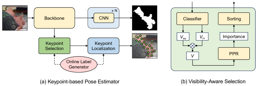
As shown in Fig. 3, we use a backbone network to extract image features from input region of interest (RoI) $I_{O}$ of object $O$. Then we utilize a multi-label classifier to predict external visibility $V_{\mathrm{ex}}(\mathbf{p})$ and internal visibility $V_{\mathrm{in}}(\mathbf{p})$ for each keypoint $\mathbf{p}\in\mathcal{P}$. Each decomposed visibility focuses on a specific factor as discussed in Sec. 3.1. Within the classifier, we adopt a shallow GNN on $k$-NN graph $G$ described in Sec. 3.3, to improve the classification consistency for connected keypoints. After estimating $V_{\mathrm{ex}}(\mathbf{p}),V_{\mathrm{in}}(\mathbf{p})$, we can get overall binary visibility $V(\mathbf{p})$ by simply multiplying $V_{\mathrm{ex}}(\mathbf{p})$ and $V_{\mathrm{in}}(\mathbf{p})$. From the predicted binary visibility of each keypoint, we generate real-valued visibility-aware importance using PPR based algorithm (Eq. 10). The coefficient matrix $\mathbf{T}_{\mathrm{PPR}}$ is precomputed using Eq. 11, so we only need to create restart vector $\mathbf{s}$ from binary visibility (Eq. 9) and run a simple matrix-vector multiplication. We then select $N^{\prime}=N/2$ keypoints with highest importance, denoted as $\mathcal{P}_{\mathrm{vis}}\subset\mathcal{P}$. We use the subgraph $G_{\mathrm{vis}}$ of $G$ induced by $\mathcal{P}_{\mathrm{vis}}$ in GNN-based localization process.

We further enhance keypoint embedding to improve the network performance. Specifically, We use a shallow GNN to obtain $64$-dim embedding $F_{P}$ from the coordinates of $\mathcal{P}$, and concatenate it with initial keypoint embedding in $G$. We can regard $F_{P}$ as positional encoding [37, 57], which facilitates the localization of the dynamic subgraph $G_{\mathrm{vis}}$.

3.5 Two-stage Training

We train our visibility-aware pose estimator in a supervised manner. As shown in Fig. 3, with object-level annotations, we generate binary labels of visibility described in Sec. 3.1 on the fly during training. Note that other supervision signals are either directly available (e.g., segmentation masks) or can also be efficiently generated on the fly (e.g., binary codes representing 2D locations).

While the whole network can be trained from scratch, it is often inefficient since the graph $G_{\mathrm{vis}}$ may vary significantly for the same input image $I$ when visibility prediction is unstable. We instead use a two-stage training procedure inspired by CheckerPose [31]. At the first stage, we train network layers corresponding to low-level estimations, including external visibility $V_{\mathrm{ex}}$, internal visibility $V_{\mathrm{in}}$, 1-bit indicator code $\mathbf{b_{v}}$, and the first $d_{0}$ bits of $\mathbf{b_{x}},\mathbf{b_{y}}$ ($\mathbf{b_{v}},\mathbf{b_{x}}$ and $\mathbf{b_{y}}$ are defined in CheckerPose). We treat the prediction of these low-level quantities as binary classification tasks, and use binary cross-entropy loss for training. At the second stage, we train the whole network. We use binary cross-entropy loss for visibility estimation and binary code generation, and apply $L_{1}$ loss for segmentation mask prediction.

4 Experiments

4.1 Experimental Setup

Implementation Details. We implement our method using PyTorch [43]. We train our network using the Adam optimizer [25] with a batch size of 32 and learning rate of 2e-4. We adopt CheckerPose [31] as our base keypoint localization method, and follow it to use $N=512$ predefined keypoints and $k=20$ nearest neighbors for $k$-NN graph. We select $N^{\prime}=256$ keypoints and use the induced subgraph in the localization step. For the binary code generation, we set the number of bits $d$ as 7, and the number of initial bits $d_{0}$ as 3. We use Progressive-X [2] to obtain pose from the correspondences for all experiments.

Datasets. Following the common practice, we conduct extensive experiments on Linemod (LM) [11], Linemod-Occlusion (LM-O) [3], and YCB-V [68]. LM contains 13 objects, and provides around $1,200$ real images for each object with mild occlusions. Following [4], we use about $15\%$ images as training set and test our method on the remaining images. We also use $1,000$ synthetic training images for each object following [30, 64, 7]. LM-O contains 8 objects from LM, and uses the real images from LM as training images. The test set is composed of $1,214$ real images with severe occlusions and clutters. YCB-V contains 21 daily objects and provides more than $110,000$ real images with severe occlusions and clutters. For training on LM-O and YCB-V, we follow the recent trend [64, 54, 31] and use the physically-based rendered data [12] as additional training images.

Evaluation Metrics. We adopt the commonly-used metric ADD(-S) to evaluate the estimated poses. To compute ADD(-S) with threshold $x\%$, we transform the 3D model points using the predicted poses and the ground truth, compute the average distance between the transformed results, and check whether the average distance is below $x\%$ of the object diameter. For symmetric objects, we compute the average distance based on the closest points. On YCB-V, we follow the common practice [64, 54, 33] to report the AUC (area under curve) of ADD-S and ADD(-S) [68], where the symmetric metric is used for all objects in ADD-S but for symmetric objects only in ADD(-S). The AUC metric reflects the accumulated performance across different thresholds, and provides complementary evaluation to ADD(-S). For keypoint-based methods, we compute average localization error by comparing the predicted keypoint locations and ground truth. We also report the inlier ratio with threshold of $x$ pixels.

4.2 Visibility Prediction

Table 1: Evaluation of visibility prediction. We report average accuracy, precision, recall, and F1 score of external visibility $V_{\mathrm{ex}}$ and internal visibility $V_{\mathrm{in}}$ on three datasets.

Dataset	$V_{\mathrm{ex}}$				$V_{\mathrm{in}}$
	Acc.	Prec.	Recall	F1	Acc.	Prec.	Recall	F1
LM [11]	92.6	94.2	97.7	95.9	98.1	98.2	97.9	98.0
LM-O [3]	87.4	84.6	85.6	84.6	91.7	91.4	91.7	91.5
YCB-V [68]	91.8	94.2	94.1	94.0	95.8	95.6	95.7	95.6

We first demonstrate that visibility classification is a relatively easy task to enable reliable keypoint selection for localization. For the prediction of external visibility $V_{\mathrm{ex}}$ and internal visibility $V_{\mathrm{in}}$, we compute accuracy, precision, recall, and F1 score. All metrics are evaluated on the networks after 50k training steps in the first stage. We report average results on the three datasets in Tab. 1. As shown in Tab. 1, a simple classifier is capable of producing good estimations.

4.3 Keypoint Localization

Table 2: Evaluation of keypoint localization. We compare our method with CheckerPose [31]. We report the average localization error, and inlier ratio with two thresholds (2 pixels and 5 pixels).

Dataset	LM [11]		LM-O [3]		YCB-V [68]
	[31]	Ours	[31]	Ours	[31]	Ours
Error (pixel)	3.4	3.1	14.4	14.4	10.9	8.7
Inlier-2px (%)	44.8	67.4	19.4	24.3	8.4	15.2
Inlier-5px (%)	88.4	88.4	67.8	71.7	39.6	55.2

We evaluate keypoint localization in Tab. 2 and compare with our baseline method CheckerPose [31]. For the LM dataset where the occlusions are mild, we significantly increase the inlier ratio with the stricter threshold (2 pixels) and achieve comparable performance with threshold of 5 pixels. For the LM-O and YCB-V datasets with severe occlusions and clutters, we significantly boost the inlier ratio. The results clearly show that our visibility-aware strategy improves the quality of 3D-2D correspondences.

4.4 Ablation Study on LM Dataset

Table 3: Ablation Study on the LM Dataset.

Method	ADD(-S)			MEAN
	0.02d	0.05d	0.1d
GDR-Net [64]	35.5	76.3	93.7	68.5
SO-Pose [7]	45.9	83.1	96.0	75.0
EPro-PnP [5]	44.8	82.0	95.8	74.2
CheckerPose [31]	35.7	84.5	97.1	72.4
Ours (w/o Selection, $N=256)$	44.7	84.3	96.9	75.3
Ours (w/o Selection, $N=512)$	45.5	84.0	96.4	75.3
Ours (w/o $V_{\mathrm{ex}}$)	48.1	85.6	96.9	76.9
Ours (w/o $V_{\mathrm{in}}$)	36.0	76.0	93.9	68.6
Ours (w/o P. E.)	46.6	84.4	96.6	75.9
Ours (w/o Two-stage)	45.4	83.9	96.1	75.1
Ours ($N^{\prime}=128$)	37.6	79.4	95.6	70.9
Ours ($N^{\prime}=192$)	45.4	84.6	96.8	75.6
Ours ($N^{\prime}=320$)	48.6	85.8	97.0	77.1
Ours ($N^{\prime}=256$)	48.6	85.9	97.0	77.2

We report ablation studies on LM [11] in Tab. 3. We train a unified pose estimator for all 13 objects. We first train the layers generating low-level quantities for 50k steps with learning rate of 2e-4, then we train all network layers for 100k steps, and finally reduce the learning rate to 1e-4 and train 20k steps.

Comparison with State of the Art. As shown in Tab. 3, our method significantly improves the performance w.r.t. ADD(-S) with threshold $2\%$ and $5\%$ (denoted as 0.02d and 0.05d). This demonstrates that our visibility-aware framework can greatly increase the ratio of qualified poses w.r.t. a strict threshold. Our method achieves comparable results w.r.t. ADD(-S) with threshold $10\%$ (denoted as 0.1d). The average of the metrics is the best among all methods.

Effectiveness of Visibility-Aware Keypoint Selection. We report the performance of using a fixed set of $N$ evenly distributed keypoints in localization step in Tab. 3. The results (denoted as w/o Selection) with $N=256$ and $N=512$ degrade especially for ADD(-S) 0.02d, which clearly demonstrates the effectiveness of our visibility-aware keypoint selection scheme.

Effectiveness of Dual Visibility Estimation. Our methods select keypoints based on both external visibility $V_{\mathrm{ex}}$ and internal visibility $V_{\mathrm{in}}$. Since the external occlusion is mild in test data of LM dataset, self-occlusion is the major factor of invisibility. As shown in Tab. 3, selecting keypoints based on $V_{\mathrm{in}}$ (denoted as w/o $V_{\mathrm{ex}}$) can significantly boost the performance compared with w/o Selection. Incorporating $V_{\mathrm{ex}}$ further improves the performance.

Effectiveness of Positional Encoding. In Tab. 3, we also present the result without positional encoding (denoted as w/o P. E.). Since the selected keypoints are dynamic w.r.t. input images, we find that adding positional encoding greatly improves the performance.

Effectiveness of Two-stage Training. In Tab. 3, we also report the performance without two-stage training (denoted as w/o Two-stage). The overall performance degrades without two-stage training, since the induced subgraph $G_{\mathrm{vis}}$ is not stable when the visibility estimator does not converge.

Number of Selected Keypoints. We show the results with different number of selected keypoints ($N^{\prime}$) in Tab. 3. The performance improves when $N^{\prime}$ is gradually increased towards 256, and remains almost the same when $N^{\prime}$ is increased to 320 with more computational cost. We use $N^{\prime}=256$ in practice.

4.5 Comparison to State of the Art

Table 4: Comparison on LM-O. We report the Average Recall (%) of ADD(-S) with three thresholds: 0.02d, 0.05d, and 0.1d. We highlight the best result and the second best result in red and blue, respectively.

Method	GDR [64]	Zebra [54]	LC [33]	Checker [31]	Ours
0.02d	4.4	9.8	8.6	7.3	9.7
0.05d	31.1	44.6	44.2	43.5	46.2
0.1d	62.2	76.9	78.06	77.5	78.02
Mean	32.6	43.8	43.6	42.8	44.6

Following [64, 54, 31, 33], we train a single pose estimator for each object on LM-O and YCB-V datasets.

Experiments on LM-O. For the two-stage training procedure, we set the first stage as 50k steps and the second stage as 700k steps. We report the average recall of ADD(-S) metric with three thresholds (0.02d, 0.05d, and 0.1d) in Tab. 4, and provide the detailed results of the 8 objects in the Supplementary Material. As shown in Tab. 4, our visibility-aware keypoint localization scheme clearly boosts our base CheckerPose [31] on all three thresholds. Our method also greatly surpasses previous methods w.r.t. 0.05d threshold and the mean of three thresholds, and achieves comparable performance w.r.t. other thresholds.

Table 5: Comparison on YCB-V. We report the average ADD(-S), and AUC of ADD-S and ADD(-S). AUC values computed without and with 11-point interpolation are denoted as “w/o" and “w/ IT", respectively. “–" denotes unavailable results.

Method	ADD(-S)	AUC-S		AUC(-S)
		w/o	w/ IT	w/o	w/ IT
SegDriven [15]	39.0	–	–	–	–
S. Stage [14]	53.9	–	–	–	–
RePose [19]	62.1	88.5	–	82.0	–
GDR-Net [64]	60.1	–	91.6	–	84.4
SO-Pose [7]	56.8	–	90.9	–	83.9
Zebra [54]	80.5	90.1	–	85.3	–
DProST [41]	65.1	–	–	77.4	–
Checker [31]	81.4	91.3	95.3	86.4	91.1
Zebra-LC [33]	82.4	90.8	95.0	86.1	90.8
Ours	84.9	92.3	96.4	87.9	92.7

Experiments on YCB-V. For the two-stage training procedure, we set the first stage as 50k steps and the second stage as 250k steps. We report the average values of ADD(-S) (0.1d) and AUC metrics in Tab. 5, and provide detailed results of the 21 objects in the Supplementary Material. Our method significantly improves the pose estimation performance w.r.t. the ADD(-S). Our method also achieves the best performance w.r.t. metrics based on AUC, which indicates that our method achieves the best accumulated performance across various thresholds.

4.6 Runtime Analysis

Table 6: Runtime Analysis. The unit of time is millisecond.

Method	Corr.	PnP	Overall
Zebra [54]	13.6	304.2	317.8
Checker [31]	68.4	33.4	101.8
Ours	68.3	31.3	99.6

In Tab. 6, we report the running speed of the methods that first establish dense correspondences and then use Progressive-X [2] as PnP solver. For an input $640\times 480$ RGB image, we evaluate the speed on a desktop with an Intel 2.30GHz CPU and an NVIDIA TITAN RTX GPU. The results show clear speed advantage of our method in addition to achieving state-of-the-art accuracies.

5 Conclusion

We propose a novel visibility-aware keypoint-based method, named VAPO, for instance-level 6DoF object pose estimation. By localizing the important keypoints guided by visibility, we efficiently invest computational resources to establish more reliable 3D-2D correspondences. From object-level annotations, we generate binary keypoint visibility labels as well as real-valued visibility-aware importance, for both asymmetric and symmetric objects. The extensive experiments on LM, LM-O and YCB-V datasets demonstrate that our method significantly improves both keypoint localization and object pose estimation.

6 Supplemental Material

6.1 Implementation Details

Hyper-parameters in the Pose Solver. We use Progressive-X [2] to obtain object poses from correspondences for all experiments. We run Progressive-X for 400 iterations with the threshold of reprojection error as 2 pixels.

Object Detectors. Following the common practice [30, 64, 7, 54, 31], we use an off-the-shelf object detector to extract region of the object in interest during inference. For the LM dataset, we use Faster-RCNN [48] detector provided by [30]. For the LM-O and YCB-V datasets, we use FCOS [60] detector provided by CDPNv2 [30].

Computation of Visibility-Aware Importance. We provide a brief explanation for that $\mathbf{I}-c\mathbf{T}$ is invertible in Eq. 11. It is equivalent to prove its transpose is invertible, that is,

$$(\mathbf{I}-c\mathbf{T})^{\top}=\mathbf{I}-c\mathbf{T}^{\top}=\mathbf{I}-\frac{c}{k}\mathbf{A}$$ (12)

is invertible, by simply verifying that $\mathbf{I}-\frac{c}{k}\mathbf{A}$ is strictly diagonally dominant. In practice, we compute the coefficient matrix defined in Eq. 11 with direct computation of inverse of $\mathbf{I}-c\mathbf{T}$. We find that it works well for $N=512$ keypoints and $k=20$ in $k$-NN graph. Since $\mathbf{I}-c\mathbf{T}$ can be very sparse, one can also explore other computation options, e.g., LU decomposition.

Visibility-Aware Keypoint Selection. We use two EdgeConv layers [65], one linear layer, and sigmoid activation function to get visibility classification results from initial keypoint embeddings in the $k$-NN graph $G$. To speed up the computation, we also output the initial bits (i.e., 1-bit indicator code $\mathbf{b_{v}}$, and the first $d_{0}$ bits of $\mathbf{b_{x}},\mathbf{b_{y}}$ defined in CheckerPose [31]) at the end of these layers concurrently. Based on the visibility classification results, we compute real-valued importance for each keypoint, and select half of the keypoints with the highest importance for localization. For extreme case when the ratio of estimated visible keypoints is below a certain threshold, we directly use $N^{\prime}$ evenly distributed keypoints for robustness. In practice, we set the threshold as 20%, since we use training images which contains at least 20% visible area of the object.

6.2 Handling Symmetric Objects

In this section we provide more details of generating visibility labels for symmetric objects. Note that to be considered as a symmetric object, the object must have both symmetric geometry and symmetric texture.

Discrete Symmetry. As described in Sec. 3.2, for an object with discrete symmetry, we can enumerate the finite equivalent poses to find the one maximizing internally visible keypoints in $\mathcal{P}_{\mathrm{sym}}$. In practice, we usually just need to compare 2 equivalent poses, so the additional computational cost is negligible. To obtain $\mathcal{P}_{\mathrm{sym}}$, we uniformly sample 2,562 rotation matrices in $SO(3)$, and set $\mathbf{t}=[0,0,400]^{\top}$ (unit is mm). The principle of selecting $\mathbf{t}$ is to make the z component greater than the object diameter, thus the camera is out of the object.

Continuous Symmetry. For an object with continuous symmetry, a straightforward way is to discretize the symmetry transformations to get finite transformations, then find the desired equivalent pose just like discrete symmetry. Though this solution is feasible, it is often need to enumerate a lot of equivalent poses (much more than 2) to ensure the accuracy. We instead derive analytic formulas that are easy to evaluate.

With Eq. 4 and Eq. 5, we get

$$\begin{split}-\mathbf{d_{p}}^{(c)}\cdot\mathbf{n}_{\mathbf{p}}^{(c)}&=(\mathbf{R}\mathbf{p}+\mathbf{t})^{\top}(\mathbf{R}\mathbf{n}_{\mathbf{p}})\\ &=\mathbf{p}^{\top}\mathbf{R}^{\top}\mathbf{R}\mathbf{n}_{\mathbf{p}}+\mathbf{t}^{\top}\mathbf{R}\mathbf{n}_{\mathbf{p}}\\ &=\mathbf{p}^{\top}\mathbf{n}_{\mathbf{p}}+(\mathbf{R}^{\top}\mathbf{t})^{\top}\mathbf{n}_{\mathbf{p}},\end{split}$$ (13)

and we can see that the first term $\mathbf{p}^{\top}\mathbf{n}_{\mathbf{p}}$ is invarient w.r.t. different poses. To maximize internally visible keypoints in $\mathcal{P}_{\mathrm{sym}}$, we only need to minimize the second term $(\mathbf{R}^{\top}\mathbf{t})^{\top}\mathbf{n}_{\mathbf{p}}$ for $\mathcal{P}_{\mathrm{sym}}$.

Base case: single continuous symmetry axis, no additional discrete symmetry. For example, symmetry transformations of a textureless bowl contains continuous rotations around an axis. The symmetry transformations can be parameterized as $\mathbf{R}_{*}(\theta)$, where $*$ denotes a symmetry axis and $\theta$ is the rotation angle around the symmetry axis. For a specific transformation $\mathbf{R}_{*}(\theta)$, the corresponding transformed rotation is

$$\tilde{\mathbf{R}}=\mathbf{R}\mathbf{R}_{*}(\theta),$$ (14)

and the corresponding transformed translation remains the same, i.e.,

$$\tilde{\mathbf{t}}=\mathbf{t},$$ (15)

thus

$$(\tilde{\mathbf{R}}^{\top}\tilde{\mathbf{t}})^{\top}\mathbf{n}_{\mathbf{p}}=(\mathbf{R}_{*}(\theta)^{\top}\mathbf{R}^{\top}\mathbf{t})^{\top}\mathbf{n}_{\mathbf{p}}=\mathbf{t}^{\top}\mathbf{R}\mathbf{R}_{*}(\theta)\mathbf{n}_{\mathbf{p}}=(\mathbf{R}^{\top}\mathbf{t})^{\top}(\mathbf{R}_{*}(\theta)\mathbf{n}_{\mathbf{p}}).$$ (16)

Without loss of generality, we can assume $z$-axis is the symmetry axis. Otherwise, we can apply a simple coordinate system transformation to the object to satisfy this assumption. Consider a special case when $\mathbf{n}_{\mathbf{p}}=\mathbf{n}_{0}=[1,0,0]^{\top}$, and then

$$\mathbf{R}_{z}(\theta)\mathbf{n}_{0}=\begin{bmatrix}\cos{\theta}&-\sin{\theta}&0\\ \sin{\theta}&\cos{\theta}&0\\ 0&0&1\end{bmatrix}\begin{bmatrix}1\\ 0\\ 0\end{bmatrix}=\begin{bmatrix}\cos{\theta}\\ \sin{\theta}\\ 0\end{bmatrix},$$ (17)

and we further get

$$(\tilde{\mathbf{R}}^{\top}\tilde{\mathbf{t}})^{\top}\mathbf{n}_{0}=a\cos{\theta}+b\sin{\theta},$$ (18)

where $a,b$ are the first and second entry of $\mathbf{R}^{\top}\mathbf{t}$, respectively. By minimizing $(\tilde{\mathbf{R}}^{\top}\tilde{\mathbf{t}})^{\top}\mathbf{n}_{0}$, we minimize the quantity in Eq. 13 for the point $\mathbf{p}_{0}$ with $\mathbf{n}_{\mathbf{p}}=\mathbf{n}_{0}=[1,0,0]^{\top}$ and its neighborhood, which ensures the internal visibility of $\mathbf{p}_{0}$ and its neighborhood (i.e., $\mathcal{P}_{\mathrm{sym}}$).

For simplicity, denote

$$f(\theta)\stackrel{{\scriptstyle\text{def}}}{{=}}a\cos{\theta}+b\sin{\theta},$$ (19)

and now we need to minimize $f(\theta)$. When $a=0$, it is straightforward to get $\theta=\pi/2+[b>0]\pi$, where $[\cdot]$ is Iverson bracket outputting binary values $\{0,1\}$. When $a\neq 0$, we have

$$f^{\prime}(\theta)=-a\sin\theta+b\cos\theta,$$ (20)

and $\theta=\arctan{(b/a)}$ is one of the solutions to make $f^{\prime}(\theta)=0$. We also need to consider

$$f^{\prime\prime}(\theta)=-a\cos\theta-b\sin\theta=-a\cos\theta(1+\frac{b}{a}\tan\theta)=-a\cos\theta(1+\frac{b^{2}}{a^{2}}),$$ (21)

and let $f^{\prime\prime}(\theta)\geq 0$, thus $\theta=\arctan{(b/a)}+[a>0]\pi$. According to the above results, we get the analytical formula Eq. 6.

Variation I: single continuous symmetry axis, additional discrete symmetry. A textureless cylinder is an example of this symmetry type. We can first use the analytic formula Eq. 6 to resolve the ambiguity caused by continuous symmetry, then enumerate the finite equivalent poses of the discrete symmetry.

Variation II: multiple continuous symmetry axes. A textureless sphere is an example of this symmetry type. Without loss of generality, we can assume $y$-axis is another symmetry axis. After resolving the ambiguity caused by continuous symmetry of $z$-axis, we apply additional transformation $\mathbf{R}_{y}(\phi)$, where $\phi$ is the rotation angle around $y$-axis. The derivation of $\phi$ is very similar to $\theta$ in $\mathbf{R}_{z}(\theta)$, hence we omit it for simplicity.

6.3 Detailed Results of LM-O

We report the detailed evaluation metrics of each object on LM-O [3] in Tab. 7, Tab. 8, and Tab. 9.

6.4 Detailed Results of YCB-V

We report the detailed evaluation metrics of each object on YCB-V [68] in Tab. 10, Tab. 11, Tab. 12, Tab. 13, and Tab. 14.

6.5 Visualization of Selected Keypoints

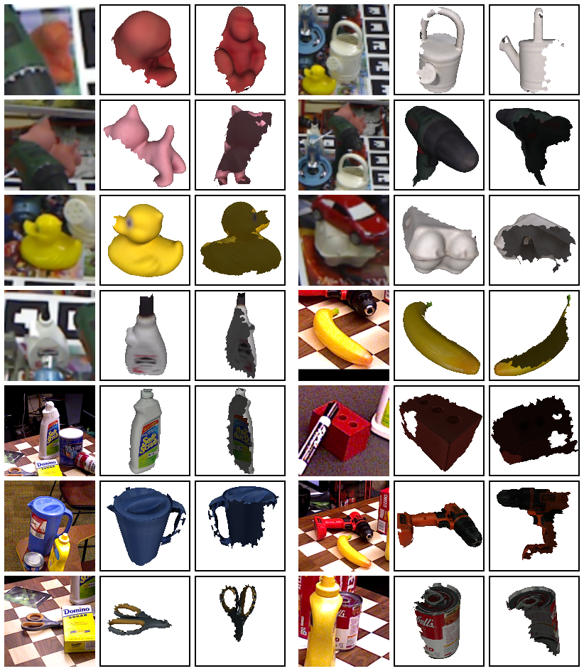
In Fig. 4, we provide qualitative results of our visibility-aware keypoint selection. Since it is hard to see the correspondences between an input image and a point cloud of selected keypoints, we compute the selection results of all vertices of the CAD models by nearest neighbor interpolation over the selection of 512 keypoints. We then visualize the faces whose vertices are all selected. We present results of various objects with different external occlusion and self-occlusion, demonstrating that our proposed visibility-aware keypoint selection module is capable of selecting reasonable keypoints for reliable 3D-2D correspondences.

6.6 Qualitative Results

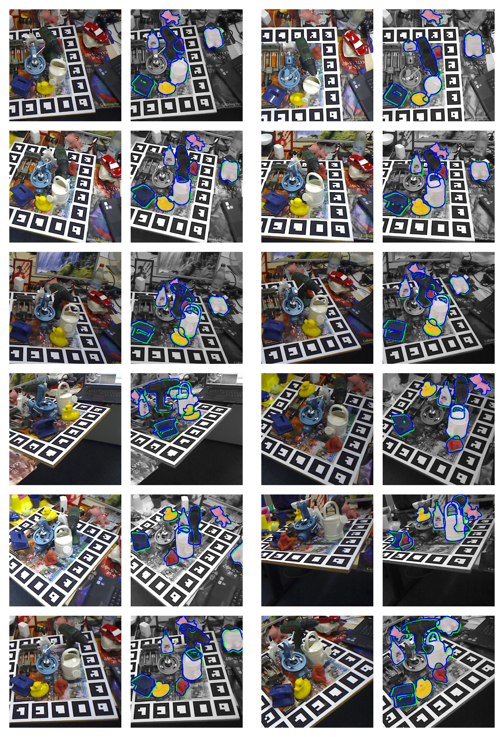
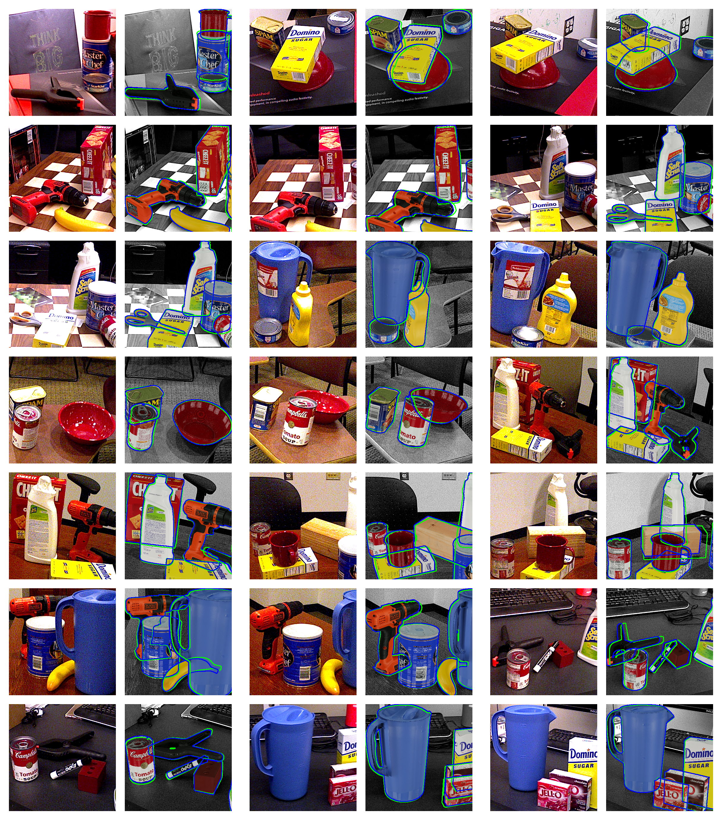
We present qualitative results of our methods for LM-O [3] and YCB-V [68] in Fig. 5 and Fig. 6, respectively.

Table 7: Average Recall (%) of ADD(-S) (0.02d) on the LM-O Dataset. (*) denotes symmetric objects.

Method	GDR [64]	Zebra [54]	LC [33]	Checker [31]	Ours
ape	0.4	0.2	0.5	0.5	0.5
can	10.8	20.7	20.9	15.6	24.0
cat	0.8	0.7	2.5	0.3	1.5
driller	12.9	19.7	20.3	10.1	20.7
duck	0.5	0.2	0.1	0.5	0.4
eggbox*	0.8	9.3	2.1	5.4	3.6
glue*	8.6	27.3	22.1	25.7	26.6
holep.	0.2	0.6	0.2	0.2	0.2
mean	4.4	9.8	8.6	7.3	9.7

Table 8: Average Recall (%) of ADD(-S) (0.05d) on the LM-O Dataset. (*) denotes symmetric objects.

Method	GDR [64]	Zebra [54]	LC [33]	Checker [31]	Ours
ape	14.2	14.4	16.5	14.0	16.5
can	66.5	79.3	81.9	79.2	82.0
cat	15.7	26.0	26.3	25.1	26.6
driller	55.6	71.2	74.3	71.4	78.6
duck	13.8	15.9	16.1	19.8	20.3
eggbox*	23.2	46.2	36.8	41.4	37.5
glue*	40.8	70.5	69.0	67.1	68.3
holep.	19.1	33.6	32.6	29.8	40.1
mean	31.1	44.6	44.2	43.5	46.2

Table 9: Average Recall (%) of ADD(-S) (0.1d) on the LM-O Dataset. (*) denotes symmetric objects.

Method	Hybrid [51]	Re [19]	GDR [64]	SO [7]	Zebra [54]	LC [33]	Checker [31]	Ours
ape	20.9	31.1	46.8	48.4	57.9	61.57	58.3	60.6
can	75.3	80.0	90.8	85.8	95.0	97.35	95.7	96.8
cat	24.9	25.6	40.5	32.7	60.6	64.49	62.3	63.1
driller	70.2	73.1	82.6	77.4	94.8	94.65	93.7	95.2
duck	27.9	43.0	46.9	48.9	64.5	66.82	69.9	66.0
eggbox*	52.4	51.7	54.2	52.4	70.9	71.77	70.0	70.5
glue*	53.8	54.3	75.8	78.3	88.7	86.35	86.4	86.2
holep.	54.2	53.6	60.1	75.3	83.0	81.49	83.8	85.7
mean	47.5	51.6	62.2	62.3	76.9	78.06	77.5	78.02

Table 10: Detailed results on YCB-V [68] w.r.t. ADD(-S) (0.1d). (*) denotes symmetric objects.

Method	Seg[15]	GDR [64]	Zebra [54]	LC [33]	Checker [31]	Ours
002_master_chef_can	33.0	41.5	62.6	51.6	45.9	45.8
003_cracker_box	44.6	83.2	98.5	99.7	94.2	99.9
004_sugar_box	75.6	91.5	96.3	99.4	98.3	99.9
005_tomato_soup_can	40.8	65.9	80.5	79.6	83.2	85.3
006_mustard_bottle	70.6	90.2	100.0	99.7	99.2	100.0
007_tuna_fish_can	18.1	44.2	70.5	86.1	88.9	82.3
008_pudding_box	12.2	2.8	99.5	99.1	86.5	77.1
009_gelatin_box	59.4	61.7	97.2	94.9	86.0	98.6
010_potted_meat_can	33.3	64.9	76.9	73.9	70.0	72.7
011_banana	16.6	64.1	71.2	95.8	96.0	93.7
019_pitcher_base	90.0	99.0	100.0	100.0	100.0	100.0
021_bleach_cleanser	70.9	73.8	75.9	85.6	89.8	89.3
024_bowl*	30.5	37.7	18.5	35.2	68.0	99.8
025_mug	40.7	61.5	77.5	88.7	89.0	95.0
035_power_drill	63.5	78.5	97.4	99.2	95.9	98.6
036_wood_block*	27.7	59.5	87.6	82.6	58.7	63.2
037_scissors	17.1	3.9	71.8	56.9	62.4	76.8
040_large_marker	4.8	7.4	23.3	27.8	18.8	25.1
051_large_clamp*	25.6	69.8	87.6	84.4	95.4	89.3
052_extra_large_clamp*	8.8	90.0	98.0	99.1	95.6	99.3
061_foam_brick*	34.7	71.9	99.3	91.3	87.2	91.3
MEAN	39.0	60.1	80.5	82.4	81.4	84.9

Table 11: Detailed results on YCB-V [68] w.r.t. AUC of ADD-S without 11-point interpolation. (*) denotes symmetric objects.

Method	Zebra [54]	LC [33]	Checker [31]	Ours
002_master_chef_can	93.7	88.4	87.5	90.9
003_cracker_box	93.0	93.7	93.2	94.4
004_sugar_box	95.1	94.7	95.9	96.2
005_tomato_soup_can	94.4	93.4	94.0	94.4
006_mustard_bottle	96.0	95.1	95.7	97.0
007_tuna_fish_can	96.9	97.2	97.5	97.2
008_pudding_box	97.2	96.7	94.9	93.9
009_gelatin_box	96.8	96.7	96.0	97.3
010_potted_meat_can	91.7	91.3	86.4	87.5
011_banana	92.6	95.3	95.7	94.7
019_pitcher_base	96.4	96.4	95.8	96.4
021_bleach_cleanser	89.5	90.5	90.6	92.6
024_bowl*	37.1	63.9	82.5	92.9
025_mug	96.1	96.5	96.9	97.3
035_power_drill	95.0	95.4	94.7	95.5
036_wood_block*	84.5	81.2	68.3	73.0
037_scissors	92.5	88.3	91.7	91.4
040_large_marker	80.4	77.6	83.3	80.0
051_large_clamp*	85.6	86.8	90.0	87.8
052_extra_large_clamp*	92.5	94.6	91.6	93.8
061_foam_brick*	95.3	93.2	94.1	94.7
MEAN	90.1	90.8	91.3	92.3

Table 12: Detailed results on YCB-V [68] w.r.t. AUC of ADD-S with 11-point interpolation. (*) denotes symmetric objects and “-" denotes unavailable results.

Method	GDR [64]	LC [33]	Checker [31]	Ours
002_master_chef_can	96.3	–	92.1	95.5
003_cracker_box	97.0	–	98.5	99.2
004_sugar_box	98.9	–	99.9	100.0
005_tomato_soup_can	96.5	–	97.2	97.6
006_mustard_bottle	100.0	–	99.9	100.0
007_tuna_fish_can	99.4	–	100.0	100.0
008_pudding_box	64.6	–	99.2	98.3
009_gelatin_box	97.1	–	99.6	100.0
010_potted_meat_can	86.0	–	89.5	90.8
011_banana	96.3	–	99.8	99.6
019_pitcher_base	99.9	–	100.0	100.0
021_bleach_cleanser	94.2	–	95.6	97.0
024_bowl*	85.7	–	85.6	99.0
025_mug	99.6	–	99.9	99.9
035_power_drill	97.5	–	99.4	99.6
036_wood_block*	82.5	–	71.9	77.4
037_scissors	63.8	–	96.5	96.1
040_large_marker	88.0	–	87.7	84.7
051_large_clamp*	89.3	–	94.7	92.6
052_extra_large_clamp*	93.5	–	96.4	98.4
061_foam_brick*	96.9	–	97.6	99.0
MEAN	91.6	95.0	95.3	96.4

Table 13: Detailed results on YCB-V [68] w.r.t. AUC of ADD(-S) without 11-point interpolation. (*) denotes symmetric objects.

Method	Zebra [54]	LC [33]	Checker [31]	Ours
002_master_chef_can	75.4	66.9	67.7	73.7
003_cracker_box	87.8	88.3	86.7	89.6
004_sugar_box	90.9	90.3	91.7	92.5
005_tomato_soup_can	90.1	89.2	89.9	90.8
006_mustard_bottle	92.6	90.9	90.9	94.2
007_tuna_fish_can	92.6	94.1	94.4	93.7
008_pudding_box	95.3	94.7	91.5	89.7
009_gelatin_box	94.8	94.6	93.4	95.5
010_potted_meat_can	83.6	82.5	80.4	80.3
011_banana	84.6	90.1	90.1	88.6
019_pitcher_base	93.4	93.2	91.9	93.2
021_bleach_cleanser	80.0	82.3	83.2	85.9
024_bowl*	37.1	63.9	82.5	92.9
025_mug	90.8	92.3	92.7	93.8
035_power_drill	89.7	90.8	88.8	90.9
036_wood_block*	84.5	81.2	68.3	73.0
037_scissors	84.5	79.0	81.6	82.7
040_large_marker	69.5	68.5	72.3	68.3
051_large_clamp*	85.6	86.8	90.0	87.8
052_extra_large_clamp*	92.5	94.6	91.6	93.8
061_foam_brick*	95.3	93.2	94.1	94.7
MEAN	85.3	86.1	86.4	87.9

Table 14: Detailed results on YCB-V [68] w.r.t. AUC of ADD(-S) with 11-point interpolation. (*) denotes symmetric objects and “-" denotes unavailable results.

Method	GDR [64]	LC [33]	Checker [31]	Ours
002_master_chef_can	65.2	–	72.0	78.2
003_cracker_box	88.8	–	91.9	94.8
004_sugar_box	95.0	–	96.9	97.6
005_tomato_soup_can	91.9	–	94.9	95.4
006_mustard_bottle	92.8	–	96.2	98.9
007_tuna_fish_can	94.2	–	99.3	98.7
008_pudding_box	44.7	–	96.7	94.5
009_gelatin_box	92.5	–	98.2	99.8
010_potted_meat_can	80.2	–	85.0	84.6
011_banana	85.8	–	95.4	93.7
019_pitcher_base	98.5	–	97.6	98.0
021_bleach_cleanser	84.3	–	88.2	91.1
024_bowl*	85.7	–	85.6	99.0
025_mug	94.0	–	97.7	98.7
035_power_drill	90.1	–	94.1	96.2
036_wood_block*	82.5	–	71.9	77.4
037_scissors	49.5	–	86.4	87.4
040_large_marker	76.1	–	77.1	73.5
051_large_clamp*	89.3	–	94.7	92.6
052_extra_large_clamp*	93.5	–	96.4	98.4
061_foam_brick*	96.9	–	97.6	99.0
MEAN	84.4	90.8	91.1	92.7

Figure 4: Visualization of selected keypoints. For better visualization, we interpolate the corresponding 3D meshes of the selected keypoints with textures. Note due to the interpolation, the boundary of the meshes may look noisy. For each input image of an object in interest, we present the mesh with two different views for comprehensive visualization.

Figure 5: Qualitative results on the LM-O dataset. For input image on the left, we visualize 6D pose on the right by rendering the 3D CAD models. Green contour denotes ground truth and blue contour denotes the prediction from our method.

Figure 6: Qualitative results on the YCB-V dataset. For each input image on the left, we visualize 6DoF pose on the right by rendering the 3D CAD models. Green contour denotes ground truth and blue contour denotes the prediction from our method.

References

- [1] Andriluka, M., Pishchulin, L., Gehler, P., Schiele, B.: 2d human pose estimation: New benchmark and state of the art analysis. In: Proceedings of the IEEE Conference on computer Vision and Pattern Recognition. pp. 3686–3693 (2014)
- [2] Barath, D., Matas, J.: Progressive-x: Efficient, anytime, multi-model fitting algorithm. In: Proceedings of the IEEE/CVF International Conference on Computer Vision (ICCV). pp. 3780–3788 (2019)
- [3] Brachmann, E., Krull, A., Michel, F., Gumhold, S., Shotton, J., Rother, C.: Learning 6d object pose estimation using 3d object coordinates. In: Proceedings of the European Conference on Computer Vision (ECCV). pp. 536–551. Springer (2014)
- [4] Brachmann, E., Michel, F., Krull, A., Yang, M.Y., Gumhold, S., et al.: Uncertainty-driven 6d pose estimation of objects and scenes from a single rgb image. In: Proceedings of the IEEE Conference on Computer Vision and Pattern Recognition (CVPR). pp. 3364–3372 (2016)
- [5] Chen, H., Wang, P., Wang, F., Tian, W., Xiong, L., Li, H.: EPro-PnP: generalized end-to-end probabilistic perspective-n-points for monocular object pose estimation. In: Proceedings of the IEEE/CVF Conference on Computer Vision and Pattern Recognition (CVPR). pp. 2781–2790 (2022)
- [6] Chen, R., Han, S., Xu, J., Su, H.: Visibility-aware point-based multi-view stereo network. IEEE transactions on pattern analysis and machine intelligence 43(10), 3695–3708 (2020)
- [7] Di, Y., Manhardt, F., Wang, G., Ji, X., Navab, N., Tombari, F.: SO-Pose: exploiting self-occlusion for direct 6d pose estimation. In: Proceedings of the IEEE/CVF International Conference on Computer Vision (ICCV). pp. 12396–12405 (2021)
- [8] Geng, Z., Sun, K., Xiao, B., Zhang, Z., Wang, J.: Bottom-up human pose estimation via disentangled keypoint regression. In: Proceedings of the IEEE/CVF conference on computer vision and pattern recognition. pp. 14676–14686 (2021)
- [9] Gu, C., Ren, X.: Discriminative mixture-of-templates for viewpoint classification. In: Proceedings of European Conference on Computer Vision (ECCV). pp. 408–421. Springer (2010)
- [10] Hinterstoisser, S., Cagniart, C., Ilic, S., Sturm, P., Navab, N., Fua, P., Lepetit, V.: Gradient response maps for real-time detection of textureless objects. IEEE transactions on pattern analysis and machine intelligence 34(5), 876–888 (2011)
- [11] Hinterstoisser, S., Lepetit, V., Ilic, S., Holzer, S., Bradski, G., Konolige, K., Navab, N.: Model based training, detection and pose estimation of texture-less 3d objects in heavily cluttered scenes. In: Asian Conference on Computer Vision (ACCV). pp. 548–562. Springer (2012)
- [12] Hodaň, T., Sundermeyer, M., Drost, B., Labbé, Y., Brachmann, E., Michel, F., Rother, C., Matas, J.: BOP challenge 2020 on 6D object localization. European Conference on Computer Vision Workshops (ECCVW) (2020)
- [13] Hu, P., Ramanan, D.: Bottom-up and top-down reasoning with hierarchical rectified gaussians. In: Proceedings of the IEEE Conference on Computer Vision and Pattern Recognition. pp. 5600–5609 (2016)
- [14] Hu, Y., Fua, P., Wang, W., Salzmann, M.: Single-stage 6d object pose estimation. In: Proceedings of the IEEE/CVF Conference on Computer Vision and Pattern Recognition (CVPR). pp. 2930–2939 (2020)
- [15] Hu, Y., Hugonot, J., Fua, P., Salzmann, M.: Segmentation-driven 6d object pose estimation. In: Proceedings of the IEEE/CVF Conference on Computer Vision and Pattern Recognition (CVPR). pp. 3385–3394 (2019)
- [16] Hu, Y., Speierer, S., Jakob, W., Fua, P., Salzmann, M.: Wide-depth-range 6d object pose estimation in space. In: Proceedings of the IEEE/CVF Conference on Computer Vision and Pattern Recognition (CVPR). pp. 15870–15879 (2021)
- [17] Hutchcroft, W., Li, Y., Boyadzhiev, I., Wan, Z., Wang, H., Kang, S.B.: Covispose: Co-visibility pose transformer for wide-baseline relative pose estimation in 360∘ indoor panoramas. In: European Conference on Computer Vision. pp. 615–633. Springer (2022)
- [18] Huttenlocher, D.P., Klanderman, G.A., Rucklidge, W.J.: Comparing images using the hausdorff distance. IEEE Transactions on pattern analysis and machine intelligence 15(9), 850–863 (1993)
- [19] Iwase, S., Liu, X., Khirodkar, R., Yokota, R., Kitani, K.M.: RePOSE: fast 6d object pose refinement via deep texture rendering. In: Proceedings of the IEEE/CVF International Conference on Computer Vision (ICCV). pp. 3303–3312 (2021)
- [20] Jain, R., Singh, K.K., Hemani, M., Lu, J., Sarkar, M., Ceylan, D., Krishnamurthy, B.: Vgflow: Visibility guided flow network for human reposing. In: Proceedings of the IEEE/CVF Conference on Computer Vision and Pattern Recognition (CVPR). pp. 21088–21097 (2023)
- [21] Johnson, S., Everingham, M.: Clustered pose and nonlinear appearance models for human pose estimation. In: bmvc. vol. 2, p. 5. Aberystwyth, UK (2010)
- [22] Katz, S., Tal, A.: On the visibility of point clouds. In: Proceedings of the IEEE international conference on computer vision (ICCV). pp. 1350–1358 (2015)
- [23] Katz, S., Tal, A., Basri, R.: Direct visibility of point sets. ACM Transactions On Graphics (TOG) 26(3), 24 (2007)
- [24] Kehl, W., Manhardt, F., Tombari, F., Ilic, S., Navab, N.: SSD-6D: making rgb-based 3d detection and 6d pose estimation great again. In: Proceedings of the IEEE International Conference on Computer Vision (ICCV). pp. 1521–1529 (2017)
- [25] Kingma, D.P., Ba, J.: Adam: A method for stochastic optimization. In: International Conference on Learning Representations (ICLR) (2015)
- [26] Kumar, S., Manocha, D., Garrett, B., Lin, M.: Hierarchical back-face culling. In: 7th Eurographics Workshop on Rendering. pp. 231–240. Citeseer (1996)
- [27] Lee, B., Lee, D.D.: Online learning of visibility and appearance for object pose estimation. In: 2016 IEEE/RSJ International Conference on Intelligent Robots and Systems (IROS). pp. 2792–2798. IEEE (2016)
- [28] Lepetit, V., Moreno-Noguer, F., Fua, P.: Epnp: An accurate o (n) solution to the pnp problem. International journal of computer vision 81(2), 155 (2009)
- [29] Li, S., Yan, Z., Li, H., Cheng, K.T.: Exploring intermediate representation for monocular vehicle pose estimation. In: Proceedings of the IEEE/CVF Conference on Computer Vision and Pattern Recognition (CVPR). pp. 1873–1883 (2021)
- [30] Li, Z., Wang, G., Ji, X.: CDPN: coordinates-based disentangled pose network for real-time rgb-based 6-dof object pose estimation. In: Proceedings of the IEEE/CVF International Conference on Computer Vision (ICCV). pp. 7678–7687 (2019)
- [31] Lian, R., Ling, H.: Checkerpose: Progressive dense keypoint localization for object pose estimation with graph neural network. In: Proceedings of the IEEE/CVF International Conference on Computer Vision (ICCV). pp. 14022–14033 (October 2023)
- [32] Lin, T.Y., Maire, M., Belongie, S., Hays, J., Perona, P., Ramanan, D., Dollár, P., Zitnick, C.L.: Microsoft coco: Common objects in context. In: Computer Vision–ECCV 2014: 13th European Conference, Zurich, Switzerland, September 6-12, 2014, Proceedings, Part V 13. pp. 740–755. Springer (2014)
- [33] Liu, F., Hu, Y., Salzmann, M.: Linear-covariance loss for end-to-end learning of 6d pose estimation. In: Proceedings of the IEEE/CVF International Conference on Computer Vision (ICCV). pp. 14107–14117 (October 2023)
- [34] Liu, Y., Peng, S., Liu, L., Wang, Q., Wang, P., Theobalt, C., Zhou, X., Wang, W.: Neural rays for occlusion-aware image-based rendering. In: Proceedings of the IEEE/CVF Conference on Computer Vision and Pattern Recognition (CVPR). pp. 7824–7833 (2022)
- [35] Manhardt, F., Kehl, W., Gaidon, A.: ROI-10D: monocular lifting of 2d detection to 6d pose and metric shape. In: Proceedings of the IEEE/CVF Conference on Computer Vision and Pattern Recognition (CVPR). pp. 2069–2078 (2019)
- [36] Marchand, E., Uchiyama, H., Spindler, F.: Pose estimation for augmented reality: a hands-on survey. IEEE transactions on visualization and computer graphics 22(12), 2633–2651 (2015)
- [37] Mildenhall, B., Srinivasan, P.P., Tancik, M., Barron, J.T., Ramamoorthi, R., Ng, R.: Nerf: Representing scenes as neural radiance fields for view synthesis. In: Proceedings of the European Conference on Computer Vision (ECCV) (2020)
- [38] Newell, A., Yang, K., Deng, J.: Stacked hourglass networks for human pose estimation. In: Computer Vision–ECCV 2016: 14th European Conference, Amsterdam, The Netherlands, October 11-14, 2016, Proceedings, Part VIII 14. pp. 483–499. Springer (2016)
- [39] Oberweger, M., Rad, M., Lepetit, V.: Making deep heatmaps robust to partial occlusions for 3d object pose estimation. In: Proceedings of the European Conference on Computer Vision (ECCV). pp. 119–134 (2018)
- [40] Page, L., Brin, S., Motwani, R., Winograd, T.: The pagerank citation ranking: Bring order to the web. Tech. rep., Technical report, stanford University (1998)
- [41] Park, J., Cho, N.I.: DProST: 6-dof object pose estimation using space carving and dynamic projective spatial transformer. In: Proceedings of the European Conference on Computer Vision (ECCV) (2022)
- [42] Park, K., Patten, T., Vincze, M.: Pix2Pose: pixel-wise coordinate regression of objects for 6d pose estimation. In: Proceedings of the IEEE/CVF International Conference on Computer Vision (ICCV). pp. 7668–7677 (2019)
- [43] Paszke, A., Gross, S., Massa, F., Lerer, A., Bradbury, J., Chanan, G., Killeen, T., Lin, Z., Gimelshein, N., Antiga, L., et al.: Pytorch: An imperative style, high-performance deep learning library. Advances in neural information processing systems 32, 8026–8037 (2019)
- [44] Peng, S., Liu, Y., Huang, Q., Zhou, X., Bao, H.: PVNet: pixel-wise voting network for 6dof pose estimation. In: Proceedings of the IEEE/CVF Conference on Computer Vision and Pattern Recognition (CVPR). pp. 4561–4570 (2019)
- [45] Pitteri, G., Bugeau, A., Ilic, S., Lepetit, V.: 3d object detection and pose estimation of unseen objects in color images with local surface embeddings. In: Proceedings of the Asian Conference on Computer Vision (2020)
- [46] Rad, M., Lepetit, V.: BB8: a scalable, accurate, robust to partial occlusion method for predicting the 3d poses of challenging objects without using depth. In: Proceedings of the IEEE International Conference on Computer Vision (ICCV). pp. 3828–3836 (2017)
- [47] Reddy, N.D., Vo, M., Narasimhan, S.G.: Occlusion-net: 2d/3d occluded keypoint localization using graph networks. In: Proceedings of the IEEE/CVF Conference on Computer Vision and Pattern Recognition. pp. 7326–7335 (2019)
- [48] Ren, S., He, K., Girshick, R., Sun, J.: Faster R-CNN: towards real-time object detection with region proposal networks. Advances in neural information processing systems 28, 91–99 (2015)
- [49] Rhodin, H., Robertini, N., Richardt, C., Seidel, H.P., Theobalt, C.: A versatile scene model with differentiable visibility applied to generative pose estimation. In: Proceedings of the IEEE International Conference on Computer Vision. pp. 765–773 (2015)
- [50] Shi, Y., Li, H., Yu, X.: Self-supervised visibility learning for novel view synthesis. In: Proceedings of the IEEE/CVF Conference on Computer Vision and Pattern Recognition (CVPR). pp. 9675–9684 (2021)
- [51] Song, C., Song, J., Huang, Q.: HybridPose: 6d object pose estimation under hybrid representations. In: Proceedings of the IEEE/CVF Conference on Computer Vision and Pattern Recognition (CVPR). pp. 431–440 (2020)
- [52] Srinivasan, P.P., Deng, B., Zhang, X., Tancik, M., Mildenhall, B., Barron, J.T.: NeRV: Neural reflectance and visibility fields for relighting and view synthesis. In: Proceedings of the IEEE/CVF Conference on Computer Vision and Pattern Recognition (CVPR). pp. 7495–7504 (2021)
- [53] Su, H., Qi, C.R., Li, Y., Guibas, L.J.: Render for CNN: viewpoint estimation in images using cnns trained with rendered 3d model views. In: Proceedings of the IEEE International Conference on Computer Vision (ICCV). pp. 2686–2694 (2015)
- [54] Su, Y., Saleh, M., Fetzer, T., Rambach, J., Navab, N., Busam, B., Stricker, D., Tombari, F.: ZebraPose: coarse to fine surface encoding for 6dof object pose estimation. In: Proceedings of the IEEE/CVF Conference on Computer Vision and Pattern Recognition (CVPR). pp. 6738–6748 (2022)
- [55] Sundermeyer, M., Marton, Z.C., Durner, M., Brucker, M., Triebel, R.: Implicit 3d orientation learning for 6d object detection from rgb images. In: Proceedings of the European Conference on Computer Vision (ECCV). pp. 699–715 (2018)
- [56] Tancik, M., Casser, V., Yan, X., Pradhan, S., Mildenhall, B., Srinivasan, P.P., Barron, J.T., Kretzschmar, H.: Block-NeRF: Scalable large scene neural view synthesis. In: Proceedings of the IEEE/CVF Conference on Computer Vision and Pattern Recognition (CVPR). pp. 8248–8258 (2022)
- [57] Tancik, M., Srinivasan, P.P., Mildenhall, B., Fridovich-Keil, S., Raghavan, N., Singhal, U., Ramamoorthi, R., Barron, J.T., Ng, R.: Fourier features let networks learn high frequency functions in low dimensional domains. Advances in Neural Information Processing Systems (2020)
- [58] Tang, F., Wu, Y., Hou, X., Ling, H.: 3d mapping and 6d pose computation for real time augmented reality on cylindrical objects. IEEE Transactions on Circuits and Systems for Video Technology 30(9), 2887–2899 (2019)
- [59] Tekin, B., Sinha, S.N., Fua, P.: Real-time seamless single shot 6d object pose prediction. In: Proceedings of the IEEE Conference on Computer Vision and Pattern Recognition (CVPR). pp. 292–301 (2018)
- [60] Tian, Z., Shen, C., Chen, H., He, T.: FCOS: fully convolutional one-stage object detection. In: Proceedings of the IEEE/CVF International Conference on Computer Vision (ICCV). pp. 9627–9636 (2019)
- [61] Tremblay, J., To, T., Sundaralingam, B., Xiang, Y., Fox, D., Birchfield, S.: Deep object pose estimation for semantic robotic grasping of household objects. In: Conference on Robot Learning. pp. 306–316. PMLR (2018)
- [62] Tremblay, J., Tyree, S., Mosier, T., Birchfield, S.: Indirect object-to-robot pose estimation from an external monocular rgb camera. In: 2020 IEEE/RSJ International Conference on Intelligent Robots and Systems (IROS). pp. 4227–4234. IEEE (2020)
- [63] Tulsiani, S., Malik, J.: Viewpoints and keypoints. In: Proceedings of the IEEE Conference on Computer Vision and Pattern Recognition (CVPR). pp. 1510–1519 (2015)
- [64] Wang, G., Manhardt, F., Tombari, F., Ji, X.: GDR-Net: geometry-guided direct regression network for monocular 6d object pose estimation. In: Proceedings of the IEEE/CVF Conference on Computer Vision and Pattern Recognition (CVPR). pp. 16611–16621 (2021)
- [65] Wang, Y., Sun, Y., Liu, Z., Sarma, S.E., Bronstein, M.M., Solomon, J.M.: Dynamic graph cnn for learning on point clouds. ACM Transactions On Graphics (TOG) 38(5), 1–12 (2019)
- [66] Wang, Z., Wu, S., Xie, W., Chen, M., Prisacariu, V.A.: Nerf–: Neural radiance fields without known camera parameters. arXiv preprint arXiv:2102.07064 (2021)
- [67] Wu, D., Zhuang, Z., Xiang, C., Zou, W., Li, X.: 6D-VNet: end-to-end 6-dof vehicle pose estimation from monocular RGB images. In: Proceedings of the IEEE/CVF Conference on Computer Vision and Pattern Recognition Workshops. pp. 0–0 (2019)
- [68] Xiang, Y., Schmidt, T., Narayanan, V., Fox, D.: PoseCNN: a convolutional neural network for 6d object pose estimation in cluttered scenes. In: Robotics: Science and Systems (2018)
- [69] Zakharov, S., Shugurov, I., Ilic, S.: DPOD: 6d pose object detector and refiner. In: Proceedings of the IEEE/CVF International Conference on Computer Vision (ICCV). pp. 1941–1950 (2019)
- [70] Zhang, E., Turk, G.: Visibility-guided simplification. In: IEEE Visualization, 2002. VIS 2002. pp. 267–274. IEEE (2002)
- [71] Zhang, H., Hoff III, K.E.: Fast backface culling using normal masks. In: Proceedings of the 1997 symposium on Interactive 3D graphics. pp. 103–ff (1997)
- [72] Zhao, Z., Peng, G., Wang, H., Fang, H.S., Li, C., Lu, C.: Estimating 6d pose from localizing designated surface keypoints. arXiv preprint arXiv:1812.01387 (2018)
- [73] Zheng, R., Li, P., Wang, H., Yu, T.: Learning visibility field for detailed 3d human reconstruction and relighting. In: Proceedings of the IEEE/CVF Conference on Computer Vision and Pattern Recognition (CVPR). pp. 216–226 (2023)
- [74] Zhou, L., Chen, Y., Gao, Y., Wang, J., Lu, H.: Occlusion-aware siamese network for human pose estimation. In: Computer Vision–ECCV 2020: 16th European Conference, Glasgow, UK, August 23–28, 2020, Proceedings, Part XX 16. pp. 396–412. Springer (2020)
- [75] Zhu, M., Derpanis, K.G., Yang, Y., Brahmbhatt, S., Zhang, M., Phillips, C., Lecce, M., Daniilidis, K.: Single image 3d object detection and pose estimation for grasping. In: 2014 IEEE International Conference on Robotics and Automation (ICRA). pp. 3936–3943. IEEE (2014)