Anomaly in open quantum systems and its implications on mixed-state quantum phases

Abstract

In this paper, we develop a systematic way to characterize the ’t Hooft anomaly in open quantum systems. Owing to nontrivial couplings to the environment, symmetries in such systems manifest as either strong or weak type. By representing their symmetry transformation through superoperators, we incorporate them in a unified framework and calculate their anomalies. In the case where the full symmetry group is $K\times G$, with $K$ the strong symmetry and $G$ the weak symmetry, we find that anomalies of bosonic systems are classified by $H^{d+2}(K\times G,U(1))/H^{d+2}(G,U(1))$ in $d$ spatial dimensions. To illustrate the power of anomalies in open quantum systems, we generally prove that anomaly must lead to nontrivial mixed-state quantum phases as long as the weak symmetry is imposed. Analogous to the “anomaly matching” condition ensuring nontrivial low-energy physics in closed systems, anomaly also guarantees nontrivial long-time dynamics, specifically steady states of Lindbladians, in open quantum systems. Notably, we identify a new exotic phase in $(1+1)$-D where the steady state shows no nontrivial correlation function in the bulk, but displays spontaneous symmetry breaking order on the boundary, which is enforced by anomalies. We discuss the general relations between mixed-state anomalies and such unconventional boundary correlation. Finally, we explore the generalization of the “anomaly inflow” mechanism in open quantum systems. We construct $(1+1)$-D and $(2+1)$-D Lindbladians whose steady states have mixed-state symmetry-protected-topological order in the bulk, with corresponding edge theories characterized by nontrivial anomalies.

I Introduction

Global symmetry plays a pivotal role in the realm of quantum many-body physics. One notable aspect is its associated ’t Hooft anomalies ’t Hooft (1980), which arise from an obstruction in promoting the global symmetry to a gauge symmetry. At a microscopic level, anomalies also manifest as obstructions to implementing symmetry transformation on a subregion Else and Nayak (2014), or fractionalization on symmetry defects Essin and Hermele (2013); Zou et al. (2021); Kawagoe and Levin (2021); Cheng and Seiberg (2023a); Delmastro et al. (2023). From the “anomaly matching” condition ’t Hooft (1980), the low-energy physics of systems with anomalous symmetries and the corresponding phase diagrams are strongly constrained, where a unique gapped ground state is forbidden. Instead, such systems must exhibit either gapless excitation or multiple degenerate ground states.

Traditionally, anomalies are defined for pure states. However, real physical systems are inevitably subjected to noises and dissipation from the environment. These effects are especially important for modern quantum simulation platforms and devices, which render the system in a mixed state Saffman et al. (2010); Kjaergaard et al. (2020); Bruzewicz et al. (2019). Recently, there has been increasing interest exciting developments about novel quantum phases and phase transitions in these open systems Dennis et al. (2002); Diehl et al. (2008); Sieberer et al. (2016); Diehl et al. (2010); Altman et al. (2015); Coser and Pérez-García (2019); Lu et al. (2023); de Groot et al. (2022a); Ma and Wang (2022); Ma et al. (2023); Lee et al. (2022); Zhang et al. (2022); Fan et al. (2023); Bao et al. (2023); Lee et al. (2023); Wang et al. (2023a); Chen and Grover (2023); Sang et al. (2023); Lieu et al. (2020); Wang et al. (2023b); Dai et al. (2023). The goal of this work is to generalize the notion of anomaly to open quantum systems/mixed states, and to show that it plays an equally important role as in closed systems, by uncovering its various implications on mixed-state quantum phases.

One unique aspect of open quantum systems is the enriched meaning of symmetries, i.e., one needs to distinguish the following two types of symmetries: 1. Weak symmetries, which means that the system and environment as a whole have the symmetry, but they are allowed to exchange symmetry charges. 2. Strong symmetries, meaning that the system itself has the symmetry, that is, the symmetry transformation acts trivially on the environment Buca and Prosen (2012). The different notions of symmetries render the characterization of anomalies in open quantum systems both challenging and compelling. In a very recent paper that appears during the process of this work Lessa et al. (2024), it is shown that anomalies of strong symmetries imply multipartite non-separability. However, a systematic definition or characterization of anomalies encompassing both strong and weak symmetries remains elusive. Also, more direct diagnostics of anomalies, especially those related to physical observables, are desired.

Moreover, in closed systems, it is known that anomaly can arise on the boundary of symmetry-protected topological (SPT) phases, leading to intriguing edge physics, which is known as “anomaly inflow” mechanism Callan and Harvey (1985); Chen et al. (2012); Levin and Gu (2012); Chen et al. (2013); Kapustin (2014); Kapustin and Thorngren (2014); Chen et al. (2011a). In recent studies, interesting mixed-state SPT phases involving both strong and weak symmetries are identified Ma and Wang (2023); Zhang et al. (2022); Ma et al. (2023); Ma and Turzillo (2024). However, the edge physics of these novel mixed-state topological phases remains unclear. Does the symmetry act anomalously in their boundary theories?

In this paper, we address all the above issues. Since there is no widely accepted way of gauging in open quantum systems, we take the obstruction to localize symmetry transformation as the definition of anomalies, where the symmetry transformation is generally represented by some superoperators. This approach enables us to directly compute the anomaly index of lattice systems and establish a classification scheme. Moreover, we find that a nontrivial anomaly index indeed indicates nontrivial mixed-state quantum phases, and it also plays a significant role in the bulk-boundary correspondence of mixed-state SPT phases. Most surprisingly, by constructing lattice models with anomalous symmetries, we find a new exotic mixed-state quantum phase, with all correlation functions appearing trivial in the bulk, but exhibiting spontaneous symmetry breaking (SSB) order on the boundary.

I.1 Summary of Results

Here we give an overview of the rest of the paper, highlighting the main results.

1. Section II is mainly a review of basic definitions of symmetries in open quantum systems and the definition of mixed-state quantum phases. We also introduce the symmetry superoperator representation.

2. In Section III, we systematically define and characterize mixed-state anomalies for bosonic systems when the full symmetry takes the form $\Gamma=K\times G$, where $K$ is the strong symmetry and $G$ is the weak symmetry. By generalizing the Else-Nayak approach to mixed states, we illustrate how to extract the anomaly index for open quantum systems. We show that the anomalies in $d$ spatial dimensions are classified by $H^{d+2}(\Gamma,U(1))/H^{d+2}(G,U(1))$. Particularly, there is no anomaly if only the weak symmetry is present. These findings are in exact correspondence to previous results on mixed-state SPT in one higher dimension.

3. Next, we show in Section IV that anomaly has strong constraining power on mixed-state quantum phases. Specifically, we prove the following theorem: A state with anomalous symmetry $K\times G$ cannot be prepared via a $G$-symmetric finite depth local quantum channel starting from a $G$-symmetric product state. Here “$G$-symmetric” refers to the weak symmetry condition.

4. After the general abstract discussion above, we construct concrete lattice models with anomalies in Section V. To diagnose more physical consequences of anomalies, we focus on open systems governed by Lindbladians. As a counterpart of “anomaly matching” in open quantum systems, we find that the long-time dynamics must be nontrivial when the Lindbladian preserves anomalous symmetries. For example, the steady states may spontaneously break the symmetry. Yet we also find a more exotic scenario, where there is no nontrivial correlation function in the bulk, but under open boundary conditions (OBC), the steady states exhibit nontrivial boundary correlation, which is enforced by anomalies. In Section VI we show generalities of such anomaly-enforced boundary correlations in open quantum systems.

5. Finally, in Section VII, we discuss the “anomaly inflow” mechanism in open quantum systems. That is, mixed-state anomalies can be realized on the edge of average SPT (ASPT), i.e., mixed-state SPT phases jointly protected by strong and weak symmetries. Using the decorated domain wall (DDW) method Chen et al. (2014), we construct symmetric Lindbladians to realize such phases as the steady states, which allows us to gain a clearer perspective on anomalous symmetry action in their edge theories. Moreover, the anomaly on the boundary/interface enables us to prove the separation of mixed-state phases for $(2+1)$-D ASPT, with the help of the theorem mentioned above.

II Preliminaries

II.1 Symmetries in open quantum systems

The purpose of this section is to review the strong and weak symmetry conditions for mixed states as well as quantum channels and Lindbladians, and meanwhile we also introduce some notations for later convenience.

For simplicity, throughout this paper we consider bosonic systems with internal symmetry groups $\Gamma$ of the product form $\Gamma=K\times G$, where $K(G)$ is the strong (weak) symmetry group. See below for the precise definition.

Definition 1 (Symmetries of mixed states). A density matrix $\rho$ has the $\Gamma$ symmetry iff:

$$\mathscr{U}(g)[\rho]\equiv U(g)\rho U^{\dagger}(g)=\rho,\forall g\in G$$ (1)

(weak symmetry condition) ,

$$\mathscr{U}(k)[\rho]\equiv U(k)\rho=\lambda(k)\rho,\forall k\in K$$

(strong symmetry condition) ,

where $\lambda(k)$ is a $U(1)$ phase factor that forms a representation of $K$ Ma and Wang (2023).

Following the above definition, the actions of a generic group element $\gamma=k\cdot g\in\Gamma$ is a generalized unitary transformation:

$$\mathscr{U}(\gamma)[\rho]=U(k\cdot g)\rho U^{\dagger}(g).$$ (2)

Here $U(\gamma)$ are unitary operators that form linear representations of $\Gamma$. Then it is straightforward to show that $\mathscr{U(\gamma)}$, when viewed as a linear map in the operator space, also forms a linear representation of the symmetry group. That is, $\mathscr{U}(\gamma_{1})\circ\mathscr{U}(\gamma_{2})=\mathscr{U}(\gamma_{1}\cdot\gamma_{2})$. These linear maps define symmetry actions on mixed states.

Finite-depth local channels (FDLC) are a natural generalization of finite-depth local unitary circuits (FDLUC), which describe a generic locality-preserving evolution of mixed states. As proposed in reference Hastings (2011), a general FDLC transformation can be constructed in the following steps: $a.$ Introduce additional qubits on each site (the environment), which defines an enlarged Hilbert space $\mathcal{H}^{S}_{i}\otimes\mathcal{H}^{E}_{i}$ on each site. The environment is initialized in some product state $|e\rangle_{E}$. $b.$ Apply an FDLUC to the total system $S\cup E$. $c.$ Trace out the environment. Thus a FDLC $\mathcal{N}$ can be written as

$$\mathcal{N}[\rho]=\text{Tr}_{E}\{D\rho\otimes|e\rangle_{E}\langle e|_{E}D^{\dagger}\},$$ (3)

where $D$ is a FDLUC. We note that the same channel can be realized using different purification schemes with different choices of $|e\rangle_{E}$ and $D$. Following de Groot et al. (2022b); Ma and Wang (2023); Ma et al. (2023), we define symmetries of local quantum channels as below.

Definition 2 (Symmetries of local quantum channels). A local channel $\mathcal{N}$ has $\Gamma$ symmetry iff there exists a purification scheme, such that:

$$=0,U_{E}(g)|e\rangle_{E}=\lambda_{E}(g)|e\rangle_{E},\forall g\in G$$ (4)

$$\text{(weak symmetry condition)},$$

$$[U(k)\otimes I_{E},D] =0,\forall k\in K$$

$$\text{(strong symmetry condition)},$$

where $U_{E}(g)$ is a unitary representation of $G$, and $\lambda_{E}(g)$ is a $U(1)$ phase factor that forms a $1d$ representation of $G$.

Under the above condition, it is easy to check that $\mathcal{N}\circ\mathscr{U}(\gamma)=\mathscr{U}(\gamma)\circ\mathcal{N}$, so $\mathcal{N}$ preserves the symmetry of states.

A large class of open quantum systems can be effectively described under Markov approximation, which basically assumes that the environment has no memory. Then the evolution of density matrices is governed by the celebrated Lindblad equation (also known as the quantum master equation):

$$\frac{d}{dt}\rho =\mathcal{L}[\rho]$$ (5)

$$\equiv-i[H,\rho]+\sum_{\mu}l_{\mu}\rho l_{\mu}-\frac{1}{2}\{l_{\mu}^{\dagger}l_{\mu},\rho\}.$$

Here the superoperator $\mathcal{L}$, known as the Lindbladian, is the generator of the nonequilibrium dynamics. $H$ is the Hamiltonian, and $l_{\mu}$, known as jump operators, describe coupling to the environment. Following Buca and Prosen (2012); Lieu et al. (2020), the symmetries of Lindbladians are defined as below.

Definition 3 (Symmetries of Lindbladians). A Lindbladian $\mathcal{L}$ has the $\Gamma$ symmetry iff $\mathcal{L}\circ\mathscr{U}(\gamma)=\mathscr{U}(\gamma)\circ\mathcal{L},\forall\gamma\in\Gamma$.

It is often very useful to use the following sufficient conditions to diagnose the symmetry: The Lindbladian has the $\Gamma$ symmetry if

$$\mathcal{L}\text{ is invariant under }H\rightarrow U(g)HU^{\dagger}(g),$$ (6)

$$l_{\mu}\rightarrow Ul_{\mu}U^{\dagger}(g),\forall g\in G\text{ (weak symmetry condition)}.$$

$$[U(k),H]=0,[U(k),l_{\mu}]=0,\forall k\in K,$$

$$\qquad\qquad\qquad\qquad\qquad\text{ (strong symmetry condition)}.$$

Notably, the weak symmetry condition is both sufficient and necessary.

As a final remark, we would like to emphasize one crucial difference between weak and strong symmetries: strong symmetries lead to conserved quantities, which are just the strong symmetry charges (generators); weak symmetries, on the other hand, are not tied with any conservation laws.

II.2 Mixed-state quantum phases

In this section we review the definition of mixed-state quantum phases proposed in recent papers Ma and Wang (2023); Ma et al. (2023); Sang et al. (2023). The ideas stem from Hastings’ work in 2011 Hastings (2011). First, we consider the classification of phases without symmetries.

Definition 4 (mixed-state quantum phases). Two mixed states $\rho_{1}$, $\rho_{2}$ belongs to the same phase if they are two-way connected by FDLCs, that is, $\exists$ a pair FDLCs $\mathcal{N}_{12},\mathcal{N}_{21}$, s.t. $\rho_{2}=\mathcal{N}_{12}[\rho_{1}],\rho_{1}=\mathcal{N}_{21}[\rho_{2}]$. Particularly, a state belongs to a (non)trivial phase if it is (not) two-way connected to a product state.

The above definition is clearly motivated by the classification of ground-state quantum phases of local gapped Hamiltonian under equivalence of FDLUC Chen et al. (2010, 2011b), and is thus natural for classification of mixed states with finite correlation length. One subtlety is that an FDLC generally has no inverse, so we must require the two-way connectivity. Furthermore, just as symmetries can enrich the variety of quantum phases in pure states, we can also impose symmetry conditions on the above definition of mixed-state quantum phases.

Definition 5 (Symmetric mixed-state quantum phases). Two mixed states with the $\Gamma$ symmetry belong to the same symmetric phase iff:

1. They are two-way connected by FDLCs with the $\Gamma$ symmetry.

2. Each layer of the FDLCs satisfies the $\Gamma$ symmetry.

Particularly, a state belongs to a (non)trivial $\Gamma$-symmetric phase if it can (not) be two-way connected to a $\Gamma$-symmetric product state.

Interesting mixed-state topological phases including SPT and symmetry enriched topological order (SET) have been investigated under this framework Ma and Wang (2023); Ma et al. (2023). Generically, we only consider onsite internal symmetries for mixed-state SPT and SETs, just like studies in pure states. One main reason is that for non-onsite internal symmetries, a symmetric product state may not even exist, so there is no natural choice of trivial state to start with. However, if we only impose weak symmetry conditions, $\Gamma=G$, then in principle we can allow it to have non-onsite action, and use the maximally mixed state to represent the trivial phase, which is indeed a symmetric product state.

III Microscopic definition, calculation, and classification of anomalies for mixed states

In this section we perform the Else-Nayak type analysis of symmetry actions on bosonic mixed-states. In this approach, anomalies manifest as some obstructions to implementing the symmetry transformation on a subregion. Compared to other approaches of diagnosing anomalies, this approach has several advantages:

1. Although the original definition of anomalies is an obstruction to gauging, the notion of gauging is still unclear for general open quantum systems. Hence we would like to avoid introducing gauge fields for general characterization.

2. In this approach, anomaly is manifestly a purely kinematic property of the system, as it should be. Namely, it can be determined by given locality, a tensor-product Hilbert space, and the form of symmetry generators. No further information of the dynamics, including the form of the Hamiltonian/Lindbladian/partition function is needed. This allows us to apply the power of anomaly to various types of open quantum systems. For example, the mixed states may arise as a steady state of dissipative dynamics, which can be Markovian or non-Markovian, or it may arise from many-body states subjected to (short-time) decoherence or weak measurement.

Due to the above consideration, we believe that the Else-Nayak approach is the most natural and straightforward generalization from closed systems to open systems, which requires minimum assumption. Thus we take the obstruction to implementing symmetry transformations on subregions as the definition of anomalies for mixed states.

III.1 Else-Nayak treatment of anomaly in pure states

To begin with, we briefly review the Else-Nayak approach in $(1+1)$-D bosonic closed systems with internal symmetry $\Gamma$ Else and Nayak (2014). This approach only works for symmetries with local unitary representation, i.e. the symmetry operator $U(\gamma)$ is an FDLUC. Let us first define restrictions of the symmetry transformations to a subregion $M$: $U_{M}\approx U$ inside $M$, i.e., $U_{M}$ and $U$ are the same in the interior of $M$, but are ambiguous up to some local unitaries near the boundary $\partial M$. Given the FDLUC nature of $U$, we have

$$U_{M}(\gamma_{1})U_{M}(\gamma_{2})=W(\gamma_{1},\gamma_{2})U_{M}(\gamma_{1}\gamma_{2}),$$ (7)

for some local unitary $W(\gamma_{1},\gamma_{2})$ acting on $\partial M$. The associativity of $U_{M}(\gamma_{1})U_{M}(\gamma_{2})U_{M}(\gamma_{3})$ dictates that $W$ should satisfy

$$W(\gamma_{1},\gamma_{2})W(\gamma_{1}\gamma_{2},\gamma_{3})=^{U_{M}(\gamma_{1})}W(\gamma_{2},\gamma_{3})W(\gamma_{1},\gamma_{2}\gamma_{3}),$$ (8)

where we use the shorthand notation ${}^{U_{M}}W\equiv U_{M}WU_{M}^{-1}$. Then we further restrict $W$ to the left and right end of $M$:

$$W(\gamma_{1},\gamma_{2})=W_{l}(\gamma_{1},\gamma_{2})W_{r}(\gamma_{1},\gamma_{2}).$$ (9)

$W_{l}$ and $W_{r}$ satisfies the consistent condition (8) up to a phase factor $\omega$:

$$\begin{split}&W_{l}(\gamma_{1},\gamma_{2})W_{l}(\gamma_{1}\gamma_{2},\gamma_{3})\\ =&\omega(\gamma_{1},\gamma_{2},\gamma_{3})^{U_{M}(\gamma_{1})}W_{l}(\gamma_{2},\gamma_{3})W_{l}(\gamma_{1},\gamma_{2}\gamma_{3}),\\ &W_{r}(\gamma_{1},\gamma_{2})W_{r}(\gamma_{1}\gamma_{2},\gamma_{3})\\ =&\omega^{-1}(\gamma_{1},\gamma_{2},\gamma_{3})^{U_{M}(\gamma_{1})}W_{r}(\gamma_{2},\gamma_{3})W_{r}(\gamma_{1},\gamma_{2}\gamma_{3}).\end{split}$$ (10)

From the associativity relation of $W_{l}(\gamma_{1},\gamma_{3})W_{l}(\gamma_{1}\gamma_{2},\gamma_{3})W_{l}(\gamma_{1}\gamma_{2}\gamma_{3},\gamma_{4})$, it can be shown that $\omega$ must satisfy the following 3-cocycle condition:

$$\begin{split}&\omega(\gamma_{1},\gamma_{2},\gamma_{3})\omega^{-1}(\gamma_{1}\gamma_{2},\gamma_{3},\gamma_{4})\omega(\gamma_{1},\gamma_{2}\gamma_{3},\gamma_{4})\\ &\omega^{-1}(\gamma_{1},\gamma_{1},\gamma_{3}\gamma_{4})\omega(\gamma_{2},\gamma_{3},\gamma_{4})=1.\end{split}$$ (11)

Furthermore, as $W$ is invariant under

$$\begin{split}W_{l}(\gamma_{1},\gamma_{2})&\rightarrow\beta(\gamma_{1},\gamma_{2})W_{l}(\gamma_{1},\gamma_{2}),\\ W_{r}(\gamma_{1},\gamma_{2})&\rightarrow\beta(\gamma_{1},\gamma_{2})^{-1}W_{r}(\gamma_{1},\gamma_{2}),\end{split}$$ (12)

$\omega$ is only uniquely defined modulo a 2-coboundary, i.e.,

$$\begin{split}\omega(\gamma_{1},\gamma_{2},\gamma_{3})\sim&\omega(\gamma_{1},\gamma_{2},\gamma_{3})\beta(\gamma_{1},\gamma_{2})\beta(\gamma_{1}\gamma_{2},\gamma_{3})\\ &\beta^{-1}(\gamma_{2},\gamma_{3})\beta^{-1}(\gamma_{1},\gamma_{2}\gamma_{3}).\end{split}$$ (13)

Consequently, the anomaly of internal symmetry $\Gamma$ in (1+1)-D can be classified by $[\omega^{\Gamma}]$ ($[\cdot]$ denotes an equivalence class defined in (13)), representing an element in the third cohomology group $H^{3}(\Gamma,U(1))$.

In higher dimensions, this approach only works for symmetries of the form

$$U(\gamma)=\sum_{\alpha}e^{i\mathcal{F}(\gamma)[\alpha]}|\gamma\alpha\rangle\langle\alpha|,$$ (14)

where $|\alpha\rangle$ are product states that form a complete basis of the Hilbert space in $d$ spatial dimensions, and $\alpha\rightarrow\gamma\alpha$ defines an onsite symmetry action of $\Gamma$. Under such assumptions, the similar reduction procedure can be repeated, eventually leading to a $(d+2)$-cocycle $\omega(\gamma_{1},\gamma_{2},\cdots,\gamma_{d+2})$ with equivalence modulo a $(d+1)$-coboundary. Therefore anomalies of the $\Gamma$ symmetry in $d+1$ dimensions can be classified by $H^{d+2}(\Gamma,U(1))$.

III.2 Generalization to mixed states

In this section, we further apply the Else-Nayak approach to mixed states. Here we consider bosonic systems with internal symmetries of the form $\Gamma=K\times G$, where $K,G$ denotes the strong and weak symmetry groups, respectively. In this case, the superoperator representation of symmetries we introduced in II.1 turns out to be very useful, which indicates a neat way of generalizing the Else-Nayak approach to mixed states. To start with, we consider $(1+1)$ dimensions and define restrictions of the symmetry transformations to a subregion $M$. $\mathscr{U}_{M}\approx\mathscr{U}$ inside $M$. More specifically, $\mathscr{U}_{M}(k\cdot g)[\rho]=U_{M}(k\cdot g)\rho U_{M}^{\dagger}(g)$, where $U_{M}$ is defined in Section III.1. Then (7), (8), (9), (10) can be naturally generalized into the superoperator version, as depicted in Fig.1.

$$\mathscr{U}_{M}(\gamma_{1})\circ\mathscr{U}_{M}(\gamma_{2})=\mathscr{W}(\gamma_{1},\gamma_{2})\circ\mathscr{U}_{M}(\gamma_{1}\cdot\gamma_{2}),$$ (15)

$$\mathscr{W}(\gamma_{1},\gamma_{2})\circ\mathscr{W}(\gamma_{1}\gamma_{2},\gamma_{3})=^{\mathscr{U}_{M}(\gamma_{1})}\mathscr{W}(\gamma_{2},\gamma_{3})\circ\mathscr{W}(\gamma_{1},\gamma_{2}\gamma_{3}),$$ (16)

$$\mathscr{W}(\gamma_{1},\gamma_{2})=\mathscr{W}_{l}(\gamma_{1},\gamma_{2})\circ\mathscr{W}_{r}(\gamma_{1}\gamma_{2}),$$ (17)

$$\begin{split}&\mathscr{W}_{l}(\gamma_{1},\gamma_{2})\circ\mathscr{W}_{l}(\gamma_{1}\gamma_{2},\gamma_{3})\\ &=\Omega(\gamma_{1},\gamma_{2},\gamma_{3})^{\mathscr{U}_{M}(\gamma_{1})}\mathscr{W}_{l}(\gamma_{2},\gamma_{3})\circ\mathscr{W}_{l}(\gamma_{1},\gamma_{2}\gamma_{3}).\end{split}$$ (18)

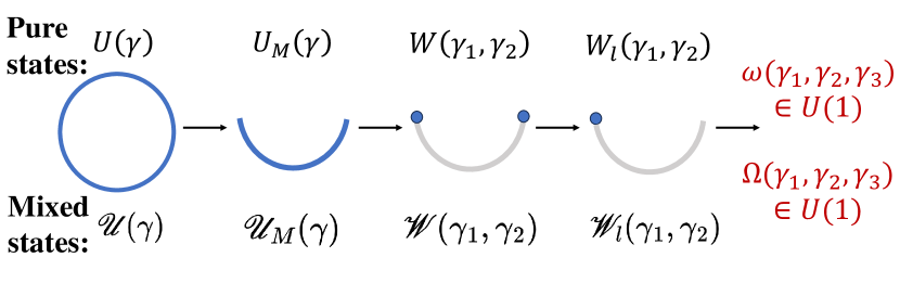
Figure 1: The dimensional reduction procedure to calculate the anomaly in $(1+1)$-D.

We use the shorthand notation ${}^{\mathscr{U}_{M}}\mathscr{W}\equiv\mathscr{U}_{M}\circ\mathscr{W}\circ\mathscr{U}^{-1}_{M}$ in Eq. (16). Naturally, the phase factor $\Omega(\gamma_{1},\gamma_{2},\gamma_{3})$ in (18) can be viewed as the anomaly indicator of the mixed states, as a generalization of the $3$-cocycle $\omega(\gamma_{1},\gamma_{2},\gamma_{3})$. Actually, $\Omega$ and $\omega$ are closely related, as we show below.

Since $\mathscr{U}_{M}$ is inherited from $U_{M}$, $\mathscr{W}$ is also determined by $W$:

$$\begin{split}&\mathscr{W}(\gamma_{1},\gamma_{2})[O]\\ &=W(\gamma_{1},\gamma_{2})OW^{\dagger}(g_{1},g_{2}),\forall\text{ operator }O\\ &=W_{l}(\gamma_{1},\gamma_{2})W_{r}(\gamma_{1},\gamma_{2})OW^{\prime\dagger}_{r}(g_{1},g_{2})W^{\prime\dagger}_{l}(g_{1},g_{2}),\end{split}$$ (19)

where $W=W_{l}W_{r}=W^{\prime}_{l}W^{\prime}_{r}$. $W_{l(r)}$ and $W^{\prime}_{l(r)}$ are identical as a function of $G$ up to a phase factor. Thus

$$\begin{split}&\mathscr{W}_{l(r)}(\gamma_{1},\gamma_{2})[O]\\ &=W_{l(r)}(\gamma_{1},\gamma_{2})OW_{l(r)}^{\prime\dagger}(g_{1},g_{2}),\forall\text{ operator }O,\end{split}$$ (20)

where we denote $\gamma_{i}=k_{i}\cdot g_{i}$. From (10) we can extract the cocycle $\omega,\omega^{\prime}$ from $W_{l},W^{\prime}_{l}$ , respectively, and (18) leads to

$$\Omega(\gamma_{1},\gamma_{2},\gamma_{3})=\omega(\gamma_{1},\gamma_{2},\gamma_{3})\omega^{\prime-1}(g_{1},g_{2},g_{3}).$$ (21)

Eq. (13) leads to the following equivalence relation of $\Omega$:

$$\begin{split}&\Omega(\gamma_{1},\gamma_{2},\gamma_{3})\sim\\ &\Omega(\gamma_{1},\gamma_{2},\gamma_{3})\beta^{\prime-1}(g_{1},g_{2})\beta^{\prime-1}(g_{1}g_{2},g_{3})\beta^{\prime}(g_{2},g_{3})\beta^{\prime}(g_{1},g_{2}g_{3})\\ &\beta(\gamma_{1},\gamma_{2})\beta(\gamma_{1}\gamma_{2},\gamma_{3})\beta^{-1}(\gamma_{2},\gamma_{3})\beta^{-1}(\gamma_{1},\gamma_{2}\gamma_{3}).\\ \end{split}$$ (22)

In other words, $[\omega^{\Gamma}]=[\omega^{\Gamma}][\omega^{G}]^{-1}$ (using the fact that $[\omega^{G}]=[\omega^{\prime G}]$).

Recall that $[\omega^{\Gamma}],[\omega^{G}]$ are elements in $H^{3}(\Gamma,U(1)),H^{3}(G,U(1))$, respectively. From the Künneth formula, the group cohomology $H^{3}(\Gamma=K\times G,U(1))$ can be decomposed as:

$$H^{3}(\Gamma,U(1))=\sum^{3}_{k=0}(H^{k}(G,H^{3-k}(K,U(1)))),$$ (23)

which contains $H^{3}(G,U(1))$ as a normal subgroup in the direct sum decomposition. Thus

$$\begin{split}[\omega^{\Gamma}]&\in H^{3}(\Gamma,U(1))/H^{3}(G,U(1))\\ &=\sum^{2}_{k=0}H^{k}(G,H^{3-k}(K,U(1))).\end{split}$$ (24)

Furthermore, for symmetries of the form in (14), we can perform the same analysis to extract the anomaly cocycle in higher dimensions

$$\begin{split}&\Omega(\gamma_{1},\gamma_{2},\cdots,\gamma_{d+2})\\ =&\omega(\gamma_{1},\gamma_{2},\cdots,\gamma_{d+2})\omega^{-1}(g_{1},g_{2},\cdots,g_{d+2}).\end{split}$$ (25)

Then

$$\begin{split}[\omega^{\Gamma}]&\in H^{d+2}(\Gamma,U(1))/H^{d+2}(G,U(1))\\ &=\sum^{d+1}_{k=0}(H^{k}(G,H^{d+2-k}(K,U(1)))).\end{split}$$ (26)

In this way we arrive at the following definition.

Definition 6. (Mixed-state anomaly) The symmetry action of $\Gamma=K\times G$ on a mixed state $\rho$ is anomalous iff $[\omega^{\Gamma}]$ is a nontrivial element in $H^{d+2}(\Gamma,U(1))/H^{d+2}(G,U(1))$, or more explicitly, it is $U(1)$ phase factor that cannot be removed by redefinition of $W_{l},W_{r}$ as in (12).

The subgroup with $k=0$ corresponds to the pure anomalies of strong symmetry $K$ while the other subgroups with $1\leq k\leq d+1$ correspond to the mixed anomalies between $K$ and $G$. Physically, this mixed anomaly can be manifested by strong symmetry fractionalization on weak symmetry defects, which we will discuss in Section V. Particularly, the absence of the $k=d+2$ term indicates that there is no anomaly with only weak symmetries. Indeed, $[\Omega]$ is always trivial when $\Gamma=G$. We will further justify this conclusion in the next section.

IV Anomaly as a tool to constrain mixed-state quantum phases

In this section, we will show that anomaly is powerful in constraining mixed-state quantum phases, which indicates that our definition of mixed-state anomalies is not only a natural one but also a useful one.

Theorem 1. A state $\rho$ with anomalous symmetry $K\times G$ cannot be prepared via a $G$-symmetric finite depth local quantum channel starting from a $G$-symmetric product state (by “$G$-symmetric” we always mean weakly symmetric). Then, according to Definition 4, $\rho$ belongs to a nontrivial $G$-symmetric phase.

Proof. We prove the contrapositive statement of the above theorem. Namely, we show that any state prepared via a $G$-symmetric FDLC from a $G$-symmetric pure product state $\rho_{0}$ must be anomaly free. Denote $\rho_{0}=\otimes_{i}\rho_{i}$, where $i$ is the site index. Then $\rho_{0}$ can be purified into the following product state: $|\psi_{SA}\rangle=\otimes_{i}|\psi_{i}\rangle=\otimes_{i}\left(\sqrt{\hat{\rho}_{i}}\otimes I^{i}_{A}\sum_{m}|m^{i}\rangle_{S}\otimes|m^{i}\rangle_{A}\right),\rho_{0}=\text{Tr}_{A}(|\psi\rangle\langle\psi|)$, where we introduce an ancilla Hilbert space $\mathcal{H}^{i}_{A}$ at each site $i$, which is isomorphic to the system Hilbert space $\mathcal{H}^{i}_{S}=span\{|m^{i}\rangle\}$ Lessa et al. (2024). Since $\rho_{0}$ is weakly symmetric, $U(g)\rho_{0}U^{\dagger}(g)=\rho_{0},\forall g\in G$, $|\psi\rangle$ also has the $G$ symmetry:

$$U(g)\otimes U^{*}(g)|\psi\rangle=|\psi\rangle.$$ (27)

Now suppose $\rho$ is prepared via the following channel:

$$\rho=\mathcal{N}[\rho_{0}]=\text{Tr}_{E}(D_{SE}\rho_{0}\otimes|0\rangle_{E}\langle 0|_{E}D_{SE}^{\dagger}),$$ (28)

where $|0_{E}\rangle$ is a $G$-symmetric product state, $U_{E}(g)|0\rangle_{E}=e^{i\theta(g)}|0\rangle_{E}$, and $D$ is some FDLUC with $G$ symmetry: $[D_{SE},U(g)\otimes U_{E}(g)]=0,\forall g\in G$.

Then $\rho$ can be purified with the help of both the ancilla (A) and the environment (E):

$$\rho=\text{Tr}_{E,A}(|\Psi\rangle\langle\Psi|),|\Psi\rangle=(D_{SE}\otimes I_{A})|\psi\rangle_{SA}\otimes|0\rangle_{E}.$$ (29)

It is easy to check that $|\Psi\rangle$ also satisfy the $G$ symmetry $U_{\text{tot}}(g)|\Psi\rangle=e^{i\theta(g)}|\Psi\rangle$, with the representation of $G$ on the total Hilbert space $\mathcal{H}^{S}\otimes\mathcal{H}^{A}\otimes\mathcal{H}^{E}$:

$$U_{\text{tot}}(g)=U(g)\otimes U^{*}(g)\otimes U_{E}(g).$$ (30)

Next, if we further require $\rho$ has strong symmetry $K$, i.e., $U(k)\rho=\lambda(k)\rho$, then $|\Psi\rangle$ also has the same $K$ symmetry charge: $U(k)\otimes I_{AE}|\Psi\rangle=\lambda(k)|\Psi\rangle$, where $AE$ is shorthand for $A\cup E$. This can be easily verified by performing the Schmidt decomposition of $|\Psi\rangle$ under the bipartition $S\cup AE$. Therefore, $|\Psi\rangle$ has the full $\Gamma=K\times G$ symmetry, where the symmetry transformation is represented by $U_{\text{tot}}(k\cdot g)=U(k\cdot g)\otimes U^{*}(g)\otimes U_{E}(g)$. We assume $U_{\text{tot}}(\gamma)$ is an FDLUC supported on a $d$-dimensional spatial region. We can extract the $(d+2)$-cocycle $\omega_{E}(g_{1},g_{2},\cdots g_{d+2}),\omega_{\text{tot}}(g_{1},g_{2},\cdots g_{d+2})$ for $U_{E}$ and $U_{\text{tot}}$, respectively, in exactly the same way as we did for $U$ in Section III.1. Due to the tensor product form of $U^{\text{tot}}$,the cocycles must satisfy the following relation:

$$\omega_{\text{tot}}(k_{1}g_{1},k_{2}g_{2},\cdots,k_{d+1}g_{d+1})$$ (31)

$$= \omega(k_{1}g_{1},k_{2}g_{2},\cdots k_{d+1}g_{d+1})$$

$$\omega^{-1}(g_{1},g_{2},\cdots,g_{d+1})\omega_{E}^{-1}(g_{1},g_{2},\cdots g_{d+1}).$$

Then, since $|\psi_{SA}\rangle\otimes|0_{E}\rangle$ is a product state and $D$ is a FDLUC, $|\Psi\rangle$ is by definition short-range entangled (SRE), and thus must be anomaly free, we can take $\omega_{\text{tot}}=1$. Take $k_{1}=k_{2}=k_{3}=1$ in (31), we obtain $\omega_{E}=1$. Then comparing (31) and (21), we get $\Omega=\omega_{\text{tot}}=1$ up to a coboundary, so $\rho$ is anomaly free.∎

We conclude this section with some remarks on the above theorem.

1. If the strong symmetry itself is anomalous, i.e., $\Omega(k_{1},k_{2},\cdots k_{d+2})(k_{i}\in K)$ represents a nontrivial element in $H^{d+2}(K,U(1))$, then we can take $G=1$ in the above theorem, which leads to the conclusion that the mixed state cannot be prepared via any FDLC from any product state. It is a straightforward generalization of the statement that a pure state preserving anomalous symmetry must be long-range entangled (LRE). We note that in this particular case a stronger result is proved in Lessa et al. (2024).

2. As mentioned at the end of Section III.2, if $\rho$ only have weak symmetry $(K=1)$, it has no anomaly. Indeed, weak symmetry has little power in constraining mixed-state quantum phases –the maximally mixed state $\rho=I$, though a trivial product state, satisfies all types of weak symmetries, $U^{\dagger}IU=I$ .

3. The most intriguing case is when the strong and weak symmetries have mixed anomalies, which is a phenomenon unique to open quantum systems. In this case, the naive generalization of ”anomaly$\Rightarrow$LRE” fails——some mixed states with mixed anomaly can still be prepared (from product states) via an FDLC, and we give such an example in the next section. Nevertheless, as proved above, such preparation is prohibited once the weak symmetry condition is imposed. We also note that even for non-onsite weak symmetry $G$, a $G$-symmetric product state always exists in the mixed state, of which the maximally mixed state is a perfect example. Thus the generality of the above theorem is guaranteed.

4. In the above proof we only assume $D$ as a whole (not each layer of it) has the $G$ symmetry. Thus the conclusion is a bit stronger than a nontrivial $G$-symmetric phase.

5. Finally but perhaps most importantly, in the above discussion a nontrivial phase is defined by impossibility of preparation via finite-depth local (symmetric) channels, based on which we establish the theorem “anomaly $\Rightarrow$ nontrivial phase ”. Then several questions arise naturally. What nontrivial phases are out there? How to diagnose them in a more direct way? For example, are there any physical quantities like correlation functions that can be used to distinguish them from trivial phases? We provide answers to these questions in the next question.

V Lattice models with anomalous symmetry in open quantum systems

In the last section, we prove that mixed states preserving anomalous symmetries must belong to a nontrivial phase. As pointed out at the end of last section, it is desirable to find concrete examples of such anomaly-enforced phases and provide a more complete and physical description of them. For this purpose, we need to go beyond the kinematic-level discussion and further input the information of dynamics. For example, in studies of quantum phases in closed systems, of particular interest is the ground state of local Hamiltonians. Then it is known that if the Hamiltonian has anomalous symmetries, the ground states are guaranteed to be nontrivial, including the following possibilities:

1. Spontaneous symmetry breaking.

2. Some local operators have a power-law correlation. In this case, the Hamiltonian has a gapless energy spectrum.

3. Topological order. This is only possible in $(2+1)$-D and higher dimensions.

In this context, we aim to establish a similar paradigm for open quantum systems. We focus on a prototypical type of dynamics, known as Markov dynamics, which means the environment is memoryless. As introduced in Section II.1 , such dynamics can be described by a Lindbladian $\mathcal{L}$. As a natural generalization of the paradigm in closed systems, we study several lattice models described by Lindbladians with anomalous symmetries, and show that as a consequence of anomalies, the steady states (defined as the zero modes of $\mathcal{L},\mathcal{L}[\rho^{ss}]=0$) indeed exhibit various anomaly-enforced nontrivial phases. Surprisingly, we identify a new type of nontrivial mixed-state phase enforced by anomalies, where correlation functions (including correlations of local operators and string order) in the bulk are all short ranged, but under OBC, the boundary states spontaneously break the symmetry. This is distinct from both scenarios in 1D pure states mentioned above. Also, it is distinct from the recently discovered mixed-state ASPT due to the lack of string order.

Below, we provide several examples of anomalous symmetries in open quantum systems. In all the examples below, we consider spin chains with a spin-1/2 degree of freedom on each site. In each example, we first define the symmetry action and demonstrate the anomaly according to our microscopic definition, and we also discuss some manifestations of anomalies. Then we construct Lindbladians with anomalous symmetries and discuss their properties.

Example 1. $K=U(1),G=\mathbb{Z}^{X}_{2}$.

Firstly, we consider the mixed anomaly between strong $U(1)$ symmetry and weak $\mathbb{Z}_{2}^{X}$ symmetry, generated by

$$Q :=\frac{1}{4}\sum_{i}(1-\sigma^{z}_{i}\sigma^{z}_{i+1}),$$ (32)

$$X :=\prod_{i}\sigma^{x}_{i},$$

respectively. Notably, the generator $Q$ counts the number of domain walls of the $\mathbb{Z}_{2}^{X}$ symmetry, and the prefactor $\frac{1}{4}$ is to ensure that $Q\in\mathbb{Z}$ under periodic boundary conditions (PBC).

To calculate the anomaly cocycle, we focus on the $\mathbb{Z}_{2}$ subgroup of U(1) symmetry which is generated by:

$$U(\text{DW})=\exp(i\pi Q)=\exp[\frac{\pi i}{4}\sum_{i}(1-\sigma^{z}_{i}\sigma^{z}_{i+1})],$$ (33)

where DW stands for domain walls. We restrict it to a subregion $M$

$$U_{M}(\text{DW})=\exp[\frac{\pi i}{4}\sum^{k-1}_{i=j}(1-\sigma^{z}_{i}\sigma^{z}_{i+1})],$$ (34)

where $M$ includes sites ${j\leq i\leq k}$. Then we find

$$(U_{M}(\text{DW}))^{2}=\sigma^{z}_{j}\sigma^{z}_{k},$$ (35)

which implies $W(\text{DW},\text{DW})=\sigma^{z}_{j}\sigma^{z}_{k}$ and $W_{l}(\text{DW},\text{DW})=\sigma^{z}_{j}$. Similarly we define $X_{M}=\prod^{k}_{i=j}\sigma^{x}_{i}$ and $U_{M}(X\text{DW})=X_{M}U_{M}(\text{DW})$. Then it follows $W_{l}(X\text{DW},X)=W_{l}(X,\text{DW})=W_{l}(I,X)=W_{l}(I,DW)=I,W_{l}(X\text{DW},X\text{DW})=W_{l}(X\text{DW},\text{DW})=\sigma^{z}_{j}$. As the weak symmetry is onsite, its cocycle $\omega^{G}$ must be in the trivial class. To determine whether $[\Omega]$ belongs to a nontrivial element in $H^{3}(K\times G,U(1))/H^{3}(G,U(1))$, we compute the following gauge invariant combination (meaning that it is invariant under (13)) of $\omega^{\Gamma}$:

$$\omega(X,\text{DW},\text{DW})\omega(X\text{DW},X,\text{DW})\omega(X\text{DW},X\text{DW},X)\cdot$$ (36)

$$\omega(X,I,X)=-1\times 1\times 1\times 1=-1.$$

Since the result is not unity and strong symmetry itself is anomaly free, it corresponds to the nontrivial cocycle in $H^{2}(G,H^{1}(K,U(1))$, signaling the mixed anomaly between $K$ and $G$.

One important and intuitive manifestation of anomaly in pure states is symmetry fractionalization on symmetry defects. Here we show that this intriguing phenomenon also shows up for mixed states, even in the case of mixed anomaly between strong and weak symmetries (the generalization to mixed states is more obvious for anomalies of purely strong symmetries), with some minor modification. Specifically, the strong symmetry fractionalizes on weak symmetry defects, which can be viewed as a physical interpretation of a nontrivial cocycle $\Omega$.

To see this, we can start with a mixed state that spontaneously breaks the weak $\mathbb{Z}_{2}^{X}$ symmetry:

$$\rho=|\uparrow\uparrow\uparrow\cdots\uparrow\rangle\langle\uparrow\uparrow\uparrow\cdots\uparrow|+|\downarrow\downarrow\downarrow\cdots\downarrow\rangle\langle\downarrow\downarrow\downarrow\cdots\downarrow|.$$ (37)

$\rho$ is invariant under the weak symmetry, $X\rho X=\rho$. However, it exhibits spontaneous weak symmetry breaking, reflected in the long range correlation $\langle\sigma_{i}^{z}\sigma_{j}^{z}\rangle=1$. $\rho$ is free of $\mathbb{Z}_{2}^{X}$ domain walls and $Q=0$. Now can we introduce weak symmetry defect (domain walls) by a string operator $\mathcal{S}=\prod_{j\leq i\leq k}\sigma^{x}_{i}$, which is a restriction of the symmetry transformation $X$ on the segment ${j\leq i\leq k}$.

$$\rho\rightarrow\rho^{\prime}=\mathcal{S}\rho\mathcal{S}$$ (38)

$$= |\uparrow\cdots\uparrow_{j}\downarrow_{j+1}\cdots\downarrow_{k}\uparrow_{k+1}\cdots\uparrow\rangle\langle\uparrow\cdots\uparrow_{j}\downarrow_{j+1}\cdots\downarrow_{k}\uparrow_{k+1}\cdots\uparrow|$$

$$+ |\downarrow\cdots\downarrow_{j}\uparrow_{j+1}\cdots\uparrow_{k}\downarrow_{k+1}\cdots\downarrow\rangle\langle\downarrow\cdots\downarrow_{j}\uparrow_{j+1}\cdots\uparrow_{k}\downarrow_{k+1}\cdots\uparrow|.$$

The string operator creates one $\mathbb{Z}_{2}^{X}$ defect at each end. It is easy to check that compared to $\rho$, the total change of $U(1)$ charge $Q$ is one. Thus each weak symmetry defect carries a half $U(1)$ charge. We note that although both the weak symmetry defect and strong symmetry charge are well-defined, there is no well-defined charge associated with weak symmetry. Thus it is questionable whether one can reversely consider weak symmetry fractionalization on strong symmetry defect. This is one major difference to anomalies in pure states.

Below, we construct Lindbladians with the anomalous $U(1)\times\mathbb{Z}_{2}^{X}$ symmetry.

$$H =\sum_{i}{J(\sigma^{x}_{i}-\sigma^{z}_{i-1}\sigma^{x}_{i}\sigma^{z}_{i+1}})-\lambda\sigma^{z}_{i}\sigma^{z}_{i+1},$$ (39)

$$l_{i} =\sqrt{r}\sigma^{z}_{i}.$$

The Hamiltonian is a prototypical realization of the edge theory of the $(2+1)$-D Levin-Gu model. The first term describes hopping of $\mathbb{Z}_{2}^{X}$ domain walls and the second term is the energy penalty of domain walls. It is invariant under both the $U(1)$ symmetry and $\mathbb{Z}_{2}^{X}$ symmetry. Here we consider the simplest form of jump operator $l_{i}$, whose effect is simply dephasing on each site. From the algebra $[Q,\sigma^{z}_{i}]=0,\{X,\sigma^{z}_{i}\}=0$, it is clear that the jump operator keeps the strong $U(1)$ symmetry and (partially) breaks the $\mathbb{Z}_{2}^{X}$ symmetry from strong to weak. Due to the strong $U(1)$ symmetry, the number of domain walls is conserved (see the end of section III). As a consequence, there must be at least one steady state in each charge sector $Q=q$ (of the $U(1)$ symmetry). Below we investigate the properties of steady state(s) in each charge sector to reveal the consequence of anomalies.

First, we discuss the case $q=0$. This scenario is extremely simple and yet illuminating. Note that there are only two states in this sector, i.e., $|\text{all up}\rangle$ and $|\text{all down}\rangle$. With dephasing, the steady states are $2$-fold: $\rho^{ss}_{1}=|\text{all up}\rangle\langle\text{all up}|,\rho^{ss}_{2}=|\text{all down}\rangle\langle\text{all down}|$. The key point is that the two steady states spontaneously break the weak $\mathbb{Z}_{2}^{X}$ symmetry, and are ferromagnetically ordered. Their symmetric combination, $\rho_{+}=\frac{|\text{all up}\rangle\langle\text{all up}|+|\text{all down}\rangle\langle\text{all down}|}{2}$, is also a valid steady state, and satisfies the weak symmetry $X\rho_{+}X=\rho_{+}$. Still, the weak symmetry breaking is reflected in the long-range correlation $\lim_{|i-j|\rightarrow\infty}\langle\sigma^{z}_{i}\sigma^{z}_{j}\rangle-\langle\sigma^{z}_{i}\rangle\langle\sigma^{z}_{j}\rangle=1$, given that $\sigma^{z}_{i}$ is odd under the $\mathbb{Z}_{2}^{X}$ transformation. From this perspective, $\rho_{+}$ can be viewed as the mixed-state counterpart of the GHZ state. The case $q=q_{\text{max}}$ (for a periodic chain with size $L$, $q_{\text{max}}=L/2$) is almost identical to $q=0$, except the steady states have Neel order in this case.

Now we turn to the more nontrivial case with intermediate densities of domain wall $q=\alpha L(0<\alpha<1/2)$. Under PBC, the steady state is unique, which is the maximally mixed state in each sector, $\rho^{ss}\propto P_{Q=q}$, where $P_{Q=q}$ is the projector to the eigenspace of $Q$ with eigenvalue $q$. It is easy to check that $\mathcal{L}[P_{Q=q}]=0$ indeed, by noting that $[P_{Q=q},l_{i}]=0,[P_{Q=q},H]=0$. In this steady state, all local operators are short-range correlated, fitting into none of the cases listed at the beginning of this section. Then how is this a nontrivial phase?

To answer this question, we investigate this model under OBC. We take

$$Q_{\text{OBC}} =\frac{1}{4}\sum_{i=1}^{L-1}(1-\sigma^{z}_{i}\sigma^{z}_{i+1}),$$ (40)

$$H_{\text{OBC}} =J\sum_{i=2}^{L-1}(\sigma^{x}_{i}-\sigma^{z}_{i-1}\sigma^{x}_{i}\sigma^{z}_{i+1})-\lambda\sum_{i=1}^{L-1}\sigma^{z}_{i}\sigma^{z}_{i+1}.$$

In this case the steady states are 2-fold degenerate for each $q$-sector.

$$\rho^{ss}_{\text{OBC},1}\propto P_{Q_{\text{OBC}}=q}(I+\sigma^{z}_{1})(I+(-1)^{2q}\sigma^{z}_{L}),$$ (41)

$$\rho^{ss}_{\text{OBC},2}=X\rho^{ss}_{\text{OBC},1}X\propto P_{Q_{\text{OBC}}=q}(I-\sigma^{z}_{1})(I-(-1)^{2q}\sigma^{z}_{L}).$$

Both $\rho^{ss}_{1},\rho^{ss}_{2}$ spontaneously breaks the weak $\mathbb{Z}^{X}_{2}$ symmetry on the boundary with nonzero magnetization, but there is no magnetization away from the boundary (in the thermodynamic limit $L\rightarrow\infty$). We can also consider their symmetric combination

$$\rho^{ss}_{\text{OBC},+} =\frac{\rho_{1}+\rho_{2}}{2}\propto P_{Q=q}(I+(-1)^{2q}\sigma^{z}_{1}\sigma^{z}_{L}),$$ (42)

$$X\rho^{ss}_{\text{OBC},+}X =\rho^{ss}_{\text{OBC},+}.$$

Then the boundary SSB is shown in the long-range correlation between the boundary spins $\langle\sigma^{z}_{1}\sigma^{z}_{L}\rangle=(-1)^{2q}$.

Although in the above we consider a particular choice of $H_{\text{OBC}}$, i.e., simply dropping terms near the boundary, we show below that the boundary SSB is actually an unavoidable consequence of the anomalous symmetry. Consider any $\rho$ that has the full $\Gamma$ symmetry: $Q_{\text{OBC}}\rho=q\rho,X\rho X=\rho$. Then

$$\langle\sigma^{z}_{1}\sigma^{z}_{L}\rangle=\langle\exp(2\pi iQ_{\text{OBC}})\rangle=(-1)^{2q}.$$ (43)

Due to the boundary SSB, for Lindbladians with the $\Gamma$ symmetry, the steady states in each $q$-sector must be at least 2-fold degenerate under OBC. Later, we will see more examples of this boundary SSB phenomenon.

Example 2. $K=\mathbb{Z}^{\text{CZ}}_{2},G=\mathbb{Z}^{X}_{2}$.

The second example is the mixed anomaly between strong $\mathbb{Z}^{\text{CZ}}_{2}$ symmetry and weak $\mathbb{Z}_{2}^{X}$ symmetry. The strong symmetry generator is

$$U(\text{CZ})=\prod_{i}\text{CZ}_{i,i+1}=\prod_{i}\exp[\frac{\pi i}{4}(1-\sigma^{z}_{i+1})(1-\sigma^{z}_{i+1})],$$ (44)

which is the product of controlled-$Z$ gates on each pair of neighboring sites. We have $[U(\text{CZ})]^{2}=1$ and $[U(\text{CZ}),X]=0$ under PBC.

To calculate the anomaly cocycle, we restrict both strong and weak symmetries to a subregion $M$

$$\begin{split}U_{M}(\text{CZ})=\exp[\sum^{k-1}_{i=j}\frac{\pi i}{4}(1-\sigma^{z}_{i})(1-\sigma^{z}_{i+1})],X_{M}=\prod^{k}_{i=j}\sigma^{x}_{i}.\end{split}$$ (45)

It is easy to check $U_{M}(\text{CZ})X_{M}=(-1)^{k-j}\sigma^{z}_{j}\sigma^{z}_{k}X_{M}U_{M}(\text{CZ})$. To identify $W$, we can restrict the combination of $U(\text{CZ})$ and $X$ to $M$ as

$$U_{M}(\text{CZ}X)=U_{M}(X\text{CZ})=U_{M}(\text{CZ})X_{M}.$$ (46)

Thus $W(\text{CZ},X)=I$ and $W(X,\text{CZ})=W(X,\text{CZ}X)=(-1)^{k-j}\sigma^{z}_{j}\sigma^{z}_{k}$. After further restriction to the left end, we can take $W_{l}(\text{CZ}X,X)=I$ and $W_{l}(X,\text{CZ})=W_{l}(X,\text{CZ}X)=(-1)^{j}\sigma^{z}_{j}$. Similarly, we also find $W_{l}(\text{CZ},\text{CZ})=W_{l}(\text{CZ},\text{CZ}X)=W_{l}(X,X)=W_{l}(I,X)=I$ and $W_{l}(\text{CZ}X,\text{CZ})=W_{l}(\text{CZ}X,\text{CZ}X)=(-1)^{j}\sigma^{z}_{j}$. Then we compute the following gauge invariant combination of $\omega^{\Gamma}$ where we replace the DW in eq (36) with CZ:

$$\omega(X,\text{CZ},\text{CZ})\omega(\text{CZ}X,X,\text{CZ})\omega(\text{CZ}X,\text{CZ}X,X)\cdot$$ (47)

$$\omega(X,I,X)=1\times(-1)\times 1\times 1=-1.$$

This nontrivial phase also signals the mixed anomaly cocycle which belongs to $H^{2}(G,H^{1}(K,U(1))$. As in the previous example, the mixed anomaly between strong $\mathbb{Z}^{\text{CZ}}_{2}$ and weak $\mathbb{Z}_{2}^{X}$ symmetry also leads to boundary SSB. Consider the symmetric state $\rho$ under OBC:

$$U_{\text{OBC}}(\text{CZ})\rho=c\rho,X\rho X=\rho,(c=\pm 1),$$ (48)

where $U_{\text{OBC}}(\text{CZ})=\exp[\sum^{L-1}_{i=1}\frac{\pi i}{4}(1-\sigma^{z}_{i})(1-\sigma^{z}_{i+1})]$. First, note that $U_{\text{OBC}}(\text{CZ})$ no longer commutes with $X$. Instead,

$$U_{\text{OBC}}(\text{CZ})XU_{\text{OBC}}(\text{CZ})=(-1)^{L-1}\sigma^{z}_{1}\sigma^{z}_{L}X.$$ (49)

Thus

$$\langle\sigma^{z}_{1}\sigma^{z}_{L}\rangle\equiv\text{Tr}(\sigma^{z}_{1}\sigma^{z}_{L}\rho)=\text{Tr}(\sigma^{z}_{1}\sigma^{z}_{L}X\rho X)$$ (50)

$$= (-1)^{L-1}\text{Tr}[U_{\text{OBC}}(\text{CZ})XU_{\text{OBC}}(\text{CZ})\rho X]$$

$$= (-1)^{L-1}.$$

Therefore, in the presence of $\mathbb{Z}_{2}^{\text{CZ}}$ symmetry, the boundary spin must break the weak $\mathbb{Z}_{2}^{X}$ symmetry. For example, we consider the following Lindbladian with the anomalous $\mathbb{Z}^{\text{CZ}}_{2}\times\mathbb{Z}_{2}^{X}$ symmetry :

$$H =\sum_{i}{J_{1}(\sigma^{x}_{i}+\sigma^{z}_{i-1}\sigma^{x}_{i}\sigma^{z}_{i+1}})$$ (51)

$$+J_{2}(\sigma^{x}_{i-1}\sigma^{x}_{i+1}+\sigma^{z}_{i-2}\sigma^{x}_{i-1}\sigma^{x}_{i+1}\sigma^{z}_{i+2}),$$

$$l_{i} =\sqrt{r}\sigma^{z}_{i}.$$

Without loss of generality, we investigate the steady state in the even $\mathbb{Z}_{2}^{\text{CZ}}$ sector, $U(\text{CZ})\rho=\rho$ and we take $L\in 2\mathbb{Z}$ . Under PBC, there is only one steady state (in this sector), which is the maximally mixed state in this sector:

$$\rho^{ss}_{\text{PBC}}\propto I+U(\text{CZ}).$$ (52)

Under OBC (as in the previous example, we define $H_{\text{OBC}}$ by dropping terms cut by the boundary), on the other hand, the steady states are $4$-fold:

$$\rho^{ss}_{\text{OBC},1} \propto(I+\sigma^{z}_{1})(I+\sigma^{z}_{L})[I+U_{\text{OBC}}(\text{CZ})],$$ (53)

$$\rho^{ss}_{\text{OBC},2} \propto(I-\sigma^{z}_{1})(I-\sigma^{z}_{L})[I+U_{\text{OBC}}(\text{CZ})],$$

$$\rho^{ss}_{\text{OBC},3} \propto(I+\sigma^{z}_{1})(I-\sigma^{z}_{L})[I+U_{\text{OBC}}(\text{CZ})],$$

$$\rho^{ss}_{\text{OBC},4} \propto(I-\sigma^{z}_{1})(I+\sigma^{z}_{L})[I+U_{\text{OBC}}(\text{CZ})].$$

They all break the $\mathbb{Z}_{2}^{X}$ symmetry on the boundary. Only the symmetric combination of $\rho^{ss}_{\text{OBC},3}$ and $\rho^{ss}_{\text{OBC},4}$ leads to a $\mathbb{Z}_{2}^{X}$ symmetric state $\rho^{ss}_{\text{OBC},+}\propto(I-\sigma^{z}_{1}\sigma^{z}_{L})[I+U_{\text{OBC}}(\text{CZ})]$, and the boundary SSB is manifested by the boundary correlation $\langle\sigma^{z}_{1}\sigma^{z}_{L}\rangle_{+}=-1$.

Despite the boundary SSB, any physical observables have trivial correlations in the bulk. To show this, we calculate the reduced density matrix for a segment $M=[\alpha L,(1-\alpha)L]$ in the bulk ($0<\alpha<\frac{1}{2}$), and find that $\rho_{M}\propto I$ in the limit $L\rightarrow\infty$. Thus the steady states of this model realize a new many-body phase, which, as far as we know, has not been discussed in previous literature. First, it resembles none of the three types of (pure-state) phases with anomalous symmetry listed at the beginning of this section. Furthermore, it is also very different from the recently proposed mixed-state SPT due to the following reasons: 1. There is no string order in the bulk; 2. According to the classification in Ma and Wang (2023); Ma et al. (2023), there is no nontrivial SPT solely protected by weak symmetries, but based on the theorem in last section, $\rho^{ss}_{\text{PBC}}$ must belong to a nontrivial mixed-state quantum phase when the weak $\mathbb{Z}_{2}^{X}$ symmetry is imposed.

Example 3. $K=\mathbb{Z}_{2}^{X},G=\mathbb{Z}_{2}^{\text{CZ}}$

In this case, as $\mathbb{Z}^{X}_{2}$ is strong symmetry while $\mathbb{Z}_{2}^{\text{CZ}}$ is weak symmetry, we simply need to exchange their positions in gauge invariant combination (47). That is

$$\omega(\text{CZ},X,X)\omega(\text{CZ}X,\text{CZ},X)\omega(\text{CZ}X,\text{CZ}X,\text{CZ})\cdot$$ (54)

$$\omega(\text{CZ},I,\text{CZ})=1\times 1\times(-1)\times 1=-1.$$

Since the cocycle of $\mathbb{Z}_{2}^{\text{CZ}}$ is also trivial, this nontrivial phase signals the mixed anomaly between $K=\mathbb{Z}^{X}_{2}$ and $G=\mathbb{Z}_{2}^{\text{CZ}}$. In this case, the boundary must break the strong $\mathbb{Z}_{2}^{X}$ symmetry under OBC. Consider the symmetric state $\rho$,

$$U_{\text{OBC}}(\text{CZ})\rho U_{\text{OBC}}=\rho,X\rho=c\rho,(c=\pm 1).$$ (55)

Then

$$\text{Tr}(\sigma^{z}_{1}\sigma^{z}_{L}\rho) =(-1)^{L-1}\text{Tr}(XU_{\text{OBC}}(\text{CZ})XU_{\text{OBC}}(\text{CZ})\rho)$$ (56)

$$=(-1)^{L-1}\text{Tr}(XU_{\text{OBC}}(\text{CZ})\rho XU_{\text{OBC}}(\text{CZ}))$$

$$=(-1)^{L-1}.$$

Below we construct a Lindbladian with the anomalous $\mathbb{Z}_{2}^{X}\times\mathbb{Z}_{2}^{\text{CZ}}$ symmetry:

$$H =\sum_{i}{J(\sigma^{x}_{i}+\sigma^{z}_{i-1}\sigma^{x}_{i}\sigma^{z}_{i+1}}),$$ (57)

$$l_{i} =\sqrt{r}(\sigma^{x}_{i}-\sigma^{z}_{i-1}\sigma^{x}_{i}\sigma^{z}_{i+1}).$$

The jump operator breaks the strong $\mathbb{Z}_{2}^{\text{CZ}}$ symmetry but preserves a residual weak $\mathbb{Z}_{2}^{\text{CZ}}$ symmetry, because $\{l_{i},U(\text{CZ})\}=0$. Below we investigate the steady state in the even $\mathbb{Z}_{2}^{X}$ sector $X=1$, and take $L\in 2\mathbb{Z}$.

Under PBC, the steady state is the maximally mixed state in this sector $\rho^{ss}_{\text{PBC}}=I+X$. This is an example where the naive generalization of “anomaly$\Rightarrow$LRE” fails, as promised in last section. Despite the anomalous $\mathbb{Z}_{2}^{X}\times\mathbb{Z}_{2}^{\text{CZ}}$ symmetry, $\rho^{ss}_{\text{PBC}}$ can be prepared via an FDLC, for example, through the following procedure:

1. Introduce an additional qubit $\tau_{i}$ on each site $i$, and initialize all spins to the $x$ direction, $\tau^{x}_{i}=\sigma^{x}_{i}=1$.

2. Apply the controlled-Z gates on onsite pairs $(\sigma_{i},\tau_{i})$ and neighboring pairs $(\tau_{i},\sigma_{i+1})$, which is a depth-$2$ LUC.

3. Trace out the $\tau$ qubits.

However, in the above construction, the initial states break the weak $\mathbb{Z}_{2}^{\text{CZ}}$ symmetry. After imposing the weak symmetry condition (to both the initial states and channels), $\rho^{ss}_{\text{PBC}}$ can no longer be prepared by FDLC. This justifies the necessity of the weak symmetry condition in Theorem 1.

Under OBC, the steady states are $2$-fold degenerate in the $X=1$ sector (and likewise in the sector $X=-1$).

$$\rho^{ss}_{\text{OBC},+} =(I+\sigma^{z}_{1}\sigma^{z}_{L})(I+X),$$ (58)

$$\rho^{ss}_{\text{OBC},-} =(I-\sigma^{z}_{1}\sigma^{z}_{L})(I+X).$$

They both show boundary SSB of the strong $\mathbb{Z}_{2}^{X}$ symmetry, $\langle\sigma^{z}_{1}\sigma^{z}_{L}\rangle_{\pm}=\pm 1$. Moreover, $\rho^{ss}_{\text{OBC},+}$ also spontaneously break the weak $\mathbb{Z}_{2}^{\text{CZ}}$ symmetry, $U_{\text{OBC}}(\text{CZ})\rho^{ss}_{\text{OBC},+}U_{\text{OBC}}(\text{CZ})=(I+\sigma^{z}_{1}\sigma^{z}_{L})(I-X)$, which is a steady state in the $X=-1$ sector. Thus the boundary weak $\mathbb{Z}_{2}^{\text{CZ}}$ SSB is responsible for the $2$-fold degeneracy in both sectors $X=\pm 1$.

Discussions. As a nontrivial consequence of anomaly, in all three examples under PBC, the $\Gamma$-symmetric steady states cannot be prepared using a $G$-symmetric FDLC from a $G$-symmetric product state. For Example 3 we explicitly show that such preparation exists if the weak symmetry condition is relaxed. However, for Example 1, 2 we do not find any way to prepare $\rho^{ss}_{\text{PBC}}$ using an FDLC from any product state. Here we conjecture that for onsite symmetry $G$, Theorem 1 could be strengthened to the following form.

Conjecture. A state $\rho$ with anomalous symmetry $K\times G$ with onsite symmetry action of $G$ cannot be prepared via any FDLC from any product state.

This conjecture is supported by the results from Ma and Wang (2023); Ma et al. (2023) that there is no SPT protected only by (onsite) weak symmetries. If any counter example of the conjecture exists, then that state can be prepared by an FDLC but is a nontrivial phase solely protected by onsite weak symmetry $G$, which would be extremely intriguing and beyond the decorated domain wall picture.

In the three examples, we leave the scenario of critical states with power law correlation. This is actually also possible for mixed states with anomalies. For example, one can start with the ground state of the Hamiltonian in (39). In the case $-1<\lambda<1$, it lies in a critical phase. Then we can apply a dephasing channel (with Kraus operator $K_{i}\propto\sigma^{z}_{i}$) to that state, breaking the strong $\mathbb{Z}_{2}^{X}$ symmetry to a weak symmetry, which still has a mixed anomaly with the strong $U(1)$ symmetry. In this case, the mixed states exhibit power law correlation, $\langle\sigma^{z}_{i}\sigma^{z}_{j}\rangle\sim\frac{1}{|i-j|^{\alpha}}(\alpha>0)$, since the dephasing channel does not change correlations between $\sigma^{z}$.

Finally, in all three examples, we encounter the boundary SSB phenomena. By making a natural choice of the symmetry operators under OBC, we show that the boundary SSB is inevitable as long as the symmetry is preserved. Then it is desirable to find out whether bondary SSB is a generic consequence of anomaly, and does not depend on how the symmetry operator is defined under OBC. For pure states, this kind of result has been proved in the context of boundary conformal field theories Wang and Wen (2023); Han et al. (2017); Jensen et al. (2018); Numasawa and Yamaguchi (2018); Li et al. (2022a); Choi et al. (2023), where anomaly is an obstruction for the existence of symmetric conformal boundary conditions. Moreover, this kind of result has been also studied in higher dimensional quantum field theories by considering fusions of symmetry defects Thorngren and Wang (2021), where anomalous symmetries must be explicitly or spontaneously broken for boundary theories. In the next section, we aim to focus on the lattice framework on $(1+1)$-D and generalize the discussion to generic mixed states.

VI Generalities of anomaly-enforced boundary correlation

In this section, we (partially) resolve the issue raised at the end of last section. Here we focus on $(1+1)$-D systems, and prove under certain conditions that anomalies would enforce nontrivial boundary correlation. First we illustrate the general ideas. Recall that anomalies are characterized by an obstruction to implementing the (truncated) symmetry transformation $\mathscr{U}_{M}$ on a subregion $M$. Under OBC, however, the symmetry (super)operator is inevitably truncated by the boundary, and thus $\mathscr{U}_{\text{OBC}}$ is just a special case of $\mathscr{U}_{M}$, and only furnish a representation of the symmetry up to some boundary obstruction. Under many circumstances, such boundary obstruction leads to nontrivial correlations between the left and right edges.

Most strikingly, we find that the above statement holds generally for anomalous strong symmetries.

Theorem 2. For an arbitrary $(1+1)$-D state $\rho$ with anomalous strong symmetry $K$, there must exist long-range boundary correlation (under OBC), i.e., $\exists$ $O_{l},O_{r}$ supported near the left and right edges, respectively, s.t. $\langle O_{l}O_{r}\rangle-\langle O_{l}\rangle\langle O_{r}\rangle\neq 0$, even in the thermodynamic limit.

Proof. As pointed out above, we can repeat the analysis in Section III.1, with $U_{M}$ replaced by $U_{\text{OBC}}$:

$$U_{\text{OBC}}(k_{1})U_{\text{OBC}}(k_{2})=W(k_{1},k_{2})U_{\text{OBC}}(k_{1}\cdot k_{2}),$$ (59)

$${U}_{\text{OBC}}(k_{1}){U}_{\text{OBC}}(k_{2})={W}(k_{1},k_{2}){U}_{\text{OBC}}(k_{1}\cdot k_{2}),$$ (60)

$${W}(k_{1},k_{2})={W}_{l}(k_{1},k_{2}){W}_{r}(k_{1}k_{2}),$$ (61)

$$\begin{split}&W_{l}(k_{1},k_{2}){W}_{l}(k_{1}k_{2},k_{3})\\ &=\omega(k_{1},k_{2},k_{3})^{{U}_{\text{OBC}}(k_{1})}{W}_{l}(k_{2},k_{3}){W}_{l}(k_{1},k_{2}k_{3}).\end{split}$$ (62)

The strong symmetry of $\rho$ states that ${U}_{\text{OBC}}(k)\rho=\lambda(k)\rho\quad(\forall k\in K)$ for some $U(1)$ phase factor $\lambda(k)$, so $\rho$ must be strongly symmetric under ${W}$: ${W}(k_{1},k_{2})\rho=\lambda(k_{1})\lambda(k_{2})\lambda^{-1}(k_{1}\cdot k_{2})\rho$.

Next, we prove by contradiction that $\exists k,k^{\prime}$, s.t. $\rho$ cannot be strongly symmetric under ${W}_{l}$. Assume that ${W}_{l}(k,k^{\prime})\rho=\beta(k,k^{\prime})\rho,\forall k,k^{\prime}\in K$, for some U(1) phase factors $\beta$. Then by applying the left hand side of (62) on $\rho$, we obtain $\omega(k_{1},k_{2},k_{3})=\beta(k_{1},k_{2})\beta(k_{1}k_{2},k_{3})\beta^{-1}(k_{1},k_{2}k_{3})\beta^{-1}(k_{2},k_{3})$, which is a 2-coboundary. It then contradicts the condition that $K$ is anomalous.

Furthermore, due to the unitarity of $W_{l}$, all of its eigenvalues are distributed on a unit circle on the complex plane, so we can conclude from the above that $\exists k,k^{\prime}\in K,|\langle W_{l}(k,k^{\prime})\rangle|\equiv|\text{Tr}(W_{l}(k,k^{\prime})\rho)|<1.$ The same goes for $W_{r}$. Therefore,

$$|\langle W_{l}(k,k^{\prime})W_{r}(k,k^{\prime})\rangle-\langle W_{l}(k,k^{\prime})\rangle\langle W_{r}(k,k^{\prime})\rangle|>0,$$ (63)

which proves the long-range correlation between left and right edges by construction. ∎

Some comments regarding the above theorem are in order. Firstly, for pure states, all symmetries are automatically strong symmetries, so the above theorem can be generally applied to pure states with anomalous symmetries . Secondly, although in Section V we focus on models with strong-weak mixed anomalies, the analysis regarding boundary SSB, e.g., (50), (56) still go through when we promote the $G$ symmetry also to a strong symmetry. For example, we can replace the dissipator in Example 1, Example 2 with $l_{i}=\sigma^{z}_{i}\sigma^{z}_{i+1}$, thus preserving the strong $\mathbb{Z}_{2}^{X}$ symmetry. Then under OBC the strong $\mathbb{Z}_{2}^{X}$ symmetry must break spontaneously on the boundary, with qubits on the two edges forming an EPR pair.

For the case with strong-weak mixed anomalies, we no longer have a proof of complete generality. Instead, we can prove the following weaker versions of the theorem.

Theorem 3. For a $(1+1)$-D state $\rho$ with anomalous symmetry $\Gamma=K\times G$, if the weak symmetry $G$ has onsite action, there must exist long-range boundary correlation, $\langle O_{l}O_{r}\rangle-\langle O_{l}\rangle\langle O_{r}\rangle\neq 0$, even in the thermodynamic limit.

The proof of Theorem 3 is almost identical to Theorem 2, and is left to Appendix A. The boundary weak $\mathbb{Z}^{X}_{2}$ SSB in Example 1, 2 are both consequences of theorem 3. For generic weak symmetry $G$, it remains unclear whether such strong conclusions still hold generally, and we are only able to show the existence of nontrivial boundary correlation in the form of Renyi-2 correlators, which is also encountered in the ”strong-to-weak SSB” phenomenon Lee et al. (2023); Ma et al. (2023). See Appendix A for discussions of this case.

VII Steady-state average SPT and anomalies of the edge theory

In closed systems, anomalies can manifest in the boundary theories of SPT phases, known as ”anomaly inflow mechanism”. Recently, SPT phases have been generalized to the open quantum systems with decoherence, under the notation of decohered average SPT (ASPT) phases . Using the decorated domain wall (DDW) approach, various types of decohered ASPT (or simply ASPT hereafter) phases are constructed and diagnosed, with a focus on their bulk properties. Notably, for symmetries of the form $\Gamma=K\times G$, the ASPT phases in $(d+2)$ spacetime dimensions are classified by $H^{d+2}(\Gamma,U(1))/H^{d+2}(G,U(1))$, which exactly coincide with our classification of mixed-state anomalies in $(d+1)$ dimensions. Therefore, it is more than natural to expect a correspondence between ASPTs and anomalies of its edge theory, generalizing the bulk-edge correspondence in closed systems.

In this section, we apply the DDW construction to Lindbladians, thus realizing ASPT in the steady states of the quantum Markov dynamics. In this way, we can facilitate a clearer and more straightforward discussion of the boundary theory and its symmetries. As an illustration, we present constructions of 2+1-dimensional $\mathbb{Z}_{2}\times\mathbb{Z}_{2}$ ASPT states in Lindbladians whose edge theories possess the same anomalous symmetries as the Example 2 and Example 3 in Section V. In appendix B, we also study an example of $(1+1)$-D steady-state ASPT.

VII.1 $(1+1)$-D $\mathbb{Z}_{2}\times\mathbb{Z}_{2}$ average SPT

As a warm up, we briefly review the construction of a $(1+1)$-D ASPT proposed in Ma and Wang (2023); Ma et al. (2023); Zhang et al. (2022); Lee et al. (2022). Consider a spin-$\frac{1}{2}$ chain with strong (weak) $\mathbb{Z}_{2}$ symmetries generated by spin flips on even (odd) sites:

$$U_{K}=\prod_{i}\sigma^{x}_{2i},\quad U_{G}=\prod_{i}\tau^{x}_{2i-1},$$ (64)

where we denote the spins on even (odd) sites as $\sigma(\tau)$. Then $\rho_{\text{trivial}}=\rho_{\sigma}^{\rightarrow}\otimes I_{\tau}$ is a trivial symmetric product state, where $\rho_{\sigma}^{\rightarrow}=\bigotimes_{i}|\sigma^{x}_{2i}=1\rangle\langle\sigma^{x}_{2i}=1|$, and $I_{\tau}$ is the maximally mixed state for $\tau$ spins. Similar to the construction of cluster state in closed systems, one can obtain a $\mathbb{Z}^{\text{strong}}_{2}\times\mathbb{Z}^{\text{weak}}_{2}$ ASPT by applying the controlled-$Z$ gates:

$$\begin{split}\rho_{\text{cluster}}=&U(\text{CZ})\rho_{\text{trivial}}U(\text{CZ})\\ =&\sum_{\{z_{2i-1}\}}\bigotimes_{i}|\tau^{z}_{2i-1}=z_{2i-1}\rangle\langle\tau^{z}_{2i-1}=z_{2i-1}|\otimes\\ &|\sigma^{x}_{2i}=z_{2i-1}z_{2i+1}\rangle\langle\sigma^{x}_{2i}=z_{2i-1}z_{2i+1}|.\end{split}$$ (65)

The above expansion indicates the DDW picture of this ASPT: a $\mathbb{Z}^{\text{strong}}_{2}$ charge is decorated on each $\mathbb{Z}_{2}^{\text{weak}}$ domain wall, which proliferates classically to restore the $\mathbb{Z}_{2}^{\text{weak}}$ symmetry. Using the DDW method, we construct a Lindbladian to realize $\rho_{\text{cluster}}$ as a steady state in Appendix B. There we show that under OBC, the $\mathbb{Z}^{\text{strong}}_{2}\times\mathbb{Z}^{\text{weak}}_{2}$ symmetry is realized projectively on the edge, which leads to a larger steady-state degeneracy compared to PBC.

VII.2 $(2+1)$-D $\mathbb{Z}_{2}\times\mathbb{Z}_{2}\times\mathbb{Z}_{2}$ and $\mathbb{Z}_{2}\times\mathbb{Z}_{2}$ average SPT

As pointed out by Ma and Wang (2023); Ma et al. (2023), one route to construct $(2+1)$-D ASPT is to decorate the $(1+1)$-D ASPT on domain walls of some other symmetry, and proliferate the domain walls. In this section we construct $(2+1)$-D steady-state ASPT by applying this idea to Lindbladians.

To begin with, we assign a spin $\frac{1}{2}$ on each vertex of a triangular lattice. We define three global $\mathbb{Z}_{2}$ (strong or weak) symmetries generated by spin-flips on the $A,B,C$ sublattices, which are colored by red, green and blue in Fig 2:

$$U_{A}=\prod_{v\in A}\sigma_{v}^{x},~{}~{}~{}~{}~{}U_{B}=\prod_{v\in B}\tau_{v}^{x},~{}~{}~{}~{}~{}U_{C}=\prod_{v\in C}\mu_{v}^{x}.$$ (66)

Figure 2: $\sigma$, $\tau$ and $\mu$ spin are assigned with vertices of $A,B,C$ sublattices, colored by red, green and blue. The green loop $N_{B}$ is on the dual lattice of $B$ sublattice and $M_{B}$ involve single $B$ vertex in its bulk. The blue loop $N_{C}$ is on the dual lattice of $C$ sublattice and $M_{C}$ involves single $C$ vertex. The two loops have two intersection points $e$ and $f$.

In the first example, we consider strong $\mathbb{Z}^{A}_{2}$ symmetry and weak $G=\mathbb{Z}^{B}_{2}\times\mathbb{Z}^{C}_{2}$ symmetry. The corresponding ASPT can be constructed by decorating the $\mathbb{Z}^{B}_{2}$ domain wall with $(1+1)$-D $\mathbb{Z}^{A}_{2}\times\mathbb{Z}^{C}_{2}$ ASPT, which is equivalent to decorating codimension-2 $\mathbb{Z}^{B}_{2}\times\mathbb{Z}^{C}_{2}$ defects with $\mathbb{Z}^{A}_{2}$ charge. Its cocycle is represented by the nontrivial element of $H^{1}(\mathbb{Z}^{B}_{2},H^{2}(\mathbb{Z}^{A}_{2}\times\mathbb{Z}^{C}_{2},U(1))=H^{2}(\mathbb{Z}^{B}_{2}\times\mathbb{Z}^{C}_{2},H^{1}(\mathbb{Z}^{A}_{2},U(1))$.

Let us start with a Lindbladian under PBC, where three types of spins are decoupled, with a trivial product state as its steady state:

$$\begin{split}&H=0,\quad l^{1}_{i\in A}=\sum_{<i,j>\in A}\sigma^{z}_{i}\sigma^{z}_{j}\frac{1-\sigma^{x}_{i}}{2},\\ &l^{2}_{i\in B/C}=\tau^{z}_{i}/\mu^{z}_{i},\quad l^{3}_{i\in B/C}=\tau^{x}_{i}/\mu^{x}_{i},\end{split}$$ (67)

where $\langle i,j\rangle\in A$ denotes nearest neighbored sites $i,j$ belonging to the sublattice $A$. . The effect of dissipators $l_{1}$ is to move or annihilate the excitation with $\sigma^{x}=-1$. Thus the steady state in the even $K$-sector has all $\sigma^{x}_{i}=1$, while in the odd $K$-sector it is the maximally mixed state of states with $\sigma^{x}=-1$ only on a single site. In other words, we have

$$\begin{split}&\rho^{ss}_{\sigma,+}=|\rightarrow\rightarrow\cdots\rightarrow\rangle\langle\rightarrow\rightarrow\cdots\rightarrow|\equiv\rho_{\sigma}^{\rightarrow},\\ &\rho^{ss}_{\sigma,-}=\frac{1}{2^{N_{\sigma}}}\sum_{i\in A}|\rightarrow\rightarrow\cdots\leftarrow_{i}\cdots\rightarrow\rangle\langle\rightarrow\rightarrow\cdots\leftarrow_{i}\cdots\rightarrow|.\end{split}$$ (68)

The effect of $l^{2}$ is to dephase on $\tau$ and $\mu$ spins and to select diagonal configurations. Then the effect of $l^{3}$ is to ensure the probability of each $\tau$ and $\mu$ configuration in steady state to be the same. Hence the steady state of $\tau$ and $\mu$ is identity $\rho^{ss}_{\tau,\mu}=I_{\tau,\mu}$. In the following discussion, we will mainly focus on the steady state in the even $K$-sector where the steady state is a trivial symmetric product state $\rho_{\text{trivial}}=\rho_{\sigma}^{\rightarrow}\otimes I_{\tau}\otimes I_{\mu}$.

In closed systems, the decoration corresponding to the nontrivial class of $H^{2}(\mathbb{Z}^{B}_{2}\times\mathbb{Z}^{C}_{2},H^{1}(\mathbb{Z}^{A}_{2},U(1))$ can be realized by a unitary transformation $U(\text{CCZ})$ Yoshida (2016); Li and Yao (2022). More precisely, $U(\text{CCZ})$ relates trivially gapped phase and $\mathbb{Z}^{A}_{2}\times\mathbb{Z}^{B}_{2}\times\mathbb{Z}^{C}_{2}$ SPT phase. Motivated by this result, we also conjugate the Lindbladian (67) by $U(\text{CCZ})$. This unitary transformation is

$$\begin{split}&U(\text{CCZ})=\prod_{(i,j,k)\in\bigtriangleup}(\text{CCZ})_{i,j,k},\\ &(\text{CCZ})_{i,j,k}|\sigma^{z}_{i}=\alpha,\tau^{z}_{j}=\beta,\mu^{z}_{k}=\gamma\rangle\\ &=(-1)^{\alpha\beta\gamma}|\sigma^{z}_{i}=\alpha,\tau^{z}_{j}=\beta,\mu^{z}_{k}=\gamma\rangle,\end{split}$$

where $\bigtriangleup$ represents the sets of all triangles and CCZ is a unitary operator acting on each triple of spins belonging to one triangle.

Then the Lindbladian after conjugated by $U_{\text{CCZ}}$ is

$$\begin{split}&l^{1}_{i\in A}=\sum_{<i,j>\in A}\sigma^{z}_{i}\sigma^{z}_{j}\frac{1-O_{i}}{2},\\ &l^{2}_{i\in B/C}=\tau^{z}_{i}/\mu^{z}_{i},\quad l^{3}_{i\in B/C}=O_{i},\end{split}$$ (69)

with steady state $\rho^{ss}_{\text{ASPT}}=U(\text{CCZ})\rho_{\text{trivial}}U^{\dagger}(\text{CCZ})$. Here $O_{i}$ operator is represented in Fig. 3 including CZ operators on all links $e$ surround the vertex $i$ (also known as the 1-links of vertex $i$):

$$\begin{split}&O_{i\in A}=\sigma^{x}_{i}\prod_{e\in 1-\text{link}(i)}\text{CZ}_{e},\\ &O_{i\in B}=\tau^{x}_{i}\prod_{e\in 1-\text{link}(i)}\text{CZ}_{e},\\ &O_{i\in C}=\mu^{x}_{i}\prod_{e\in 1-\text{link}(i)}\text{CZ}_{e}.\end{split}$$

Hence, the dissipator $l^{1}$ enforces steady states satisfying $O_{i\in A}=1$, which we will study its SPT feature later. Next, the effect of $l^{2}$ is dephasing on $\tau,\sigma$ spins, which selects diagonal domain wall configuration. Finally, $l^{3}$ will incoherently proliferate the domain wall configuration in a way compatible with the decoration pattern, since $[l^{3},O_{i\in A}]=0$.

To detect the SPT feature of steady states, we consider a $\mathbb{Z}^{B}_{2}$ domain wall supported in a closed loop $N_{B}$ in the dual lattice of $B$, namely $A$ and $C$ sublattice. Such the domain wall can be constructed by conjugating the steady state using $\prod_{i\in M_{B}}\tau^{x}_{i}$, where $M_{B}$ involves $B$ sites enclosed by $N_{B}$, as shown in Fig. 2. It is straightforward to check

$$\begin{split}&\prod_{M_{B}}\tau^{x}_{i}\rho^{ss}_{\text{ASPT}}\prod_{M_{B}}\tau^{x}_{i}\\ =&U(\text{CCZ})U_{N_{B}}(\text{CZ})\prod_{i\in M_{B}}\tau^{x}_{i}\rho_{\text{trivial}}\prod_{i\in M_{B}}\tau^{x}_{i}U^{\dagger}_{N_{B}}(\text{CZ})U^{\dagger}(\text{CCZ})\\ =&U(\text{CCZ})U_{N_{B}}(\text{CZ})\rho_{\text{trivial}}U^{\dagger}_{N_{B}}(\text{CZ})U^{\dagger}(\text{CCZ})\\ =&U_{N_{B}}(\text{CZ})\rho^{ss}_{\text{ASPT}}U^{\dagger}_{N_{B}}(\text{CZ}).\end{split}$$ (70)

As shown in Section VII.1, $U(\text{CZ})$ is a duality between $(1+1)$-D trival mixed state and $\mathbb{Z}^{\text{strong}}_{2}\times\mathbb{Z}^{\text{weak}}_{2}$ ASPT. Thus Eq. (70) implies $\mathbb{Z}^{B}_{2}$ domain wall is decorated with a $(1+1)$-D $\mathbb{Z}^{A}_{2}\times\mathbb{Z}^{C}_{2}$ ASPT.

Figure 3: The local term $O_{i}$ where a Pauli $X$ operator at the vertex $i$ is decorated by CZ operators on all links surround this vertex. $X$ operator corresponds to the Pauli operator $\sigma^{x}$ or $\tau^{x}$ or $\mu^{x}$.

Figure 4: The subregion $M_{B}$ involves two $B$ vertices and $M_{C}$ involves single $C$ vertex. $N_{B}$ and $N_{C}$ are colored by green and blue respectively and have three intersection points $d$, $e$, $f$ where $s_{d}=s_{e}=1,s_{f}=2$.

Furthermore, one can continue to construct the $\mu$ domain walls on the closed loop $N_{C}$ in the dual lattice of $C$ sublattice, i.e., $A$ and $B$ sublattice. This corresponds to conjugating the steady state by $\mu$ spin flip in the subregion $M_{C}$ which involves the $C$ vertices enclosed by $N_{C}$. Let us first consider $M_{B}$ and $M_{C}$ includes two nearest neighboured sites $m,n$ as shown in Fig. 2, then we have

$$\begin{split}&\mu^{x}_{m}\tau^{x}_{n}\rho^{ss}_{\text{ASPT}}\tau^{x}_{n}\mu^{x}_{m}\\ =&\sigma^{z}_{e}\sigma^{z}_{f}U_{N_{B}\cup N_{C}}(\text{CZ})\rho^{ss}_{\text{ASPT}}U^{\dagger}_{N_{B}\cup N_{C}}(\text{CZ})\sigma^{z}_{e}\sigma^{z}_{f}.\end{split}$$ (71)

This can be easily generalized to general $M_{B}$ and $M_{C}$ as follows. For each $A$ vertex $i\in N_{B}\cap N_{C}$, if one of its 1-links, i.e., a $BC$ link surround $i$, has two endpoints belonging to $M_{B}$ and $M_{C}$ respectively, the steady state will obtain a $\sigma^{z}_{i}$ after conjugating the spin flip on the two endpoints. In other words, we have

$$\begin{split}&\prod_{M_{C}}\mu^{x}_{j}\prod_{M_{B}}\tau^{x}_{k}\rho^{ss}_{\text{ASPT}}\prod_{M_{B}}\tau^{x}_{k}\prod_{M_{C}}\mu^{x}_{j}\\ =&\prod_{N_{B}\cap N_{C}}(\sigma^{z}_{i})^{s_{i}}U_{N_{B}\cup N_{C}}(\text{CZ})\rho^{ss}_{\text{ASPT}}U^{\dagger}_{N_{B}\cup N_{C}}(\text{CZ})\prod_{N_{B}\cap N_{C}}(\sigma^{z}_{i})^{s_{i}}.\end{split}$$ (72)

Here $s_{i}$ is the number of 1-links of $A$ vertex $i$ whose endpoints are in $M_{B}$ and $M_{C}$. An example is shown in Fig. 4.

The result (72) implies the codimension-2 defects of the weak symmetry, i.e., intersection points of $\mathbb{Z}^{B}_{2}$ and $\mathbb{Z}^{C}_{2}$ domain walls with odd $s_{i}$, are decorated with $\mathbb{Z}^{A}_{2}$ charge.

Moreover, we show that the same model also realizes a nontrivial ASPT even when we only consider the sub-symmetry group $K=\mathbb{Z}^{A}_{2},G=\mathbb{Z}^{BC}_{2}$, with $\mathbb{Z}_{2}^{BC}$ generated by $U_{B}U_{C}$. In this case $\rho^{ss}_{\text{ASPT}}$ corresponds to the nontrivial class in $H^{2}(\mathbb{Z}^{BC}_{2},H^{1}(\mathbb{Z}^{A}_{2},U(1))$ in the DDW classification, as we demonstrate below.

First, due to the dissipator $l^{1}$, steady states satisfy $O_{i\in A}=1$. This indicates that the $K$ charge distribution $\{\sigma^{x}_{i}\}$ is determined by the domain wall configuration of $\mathbb{Z}_{2}^{BC}$, which is a loop $N_{BC}$ on the $A$ sublattice. More specifically, a $K$-charge ($\sigma^{x}_{i}=-1$) is decorated on each $120^{\circ}$ (or equivalently, $240^{\circ}$) corner of $\mathbb{Z}_{2}^{BC}$ domain walls, which we denote as a codimension-2 defect of the $\mathbb{Z}_{2}^{BC}$ symmetry. See Fig. 5 for an illustration. Next, $l^{2}$ and $l^{3}$ will still dephase on $\tau,\sigma$ spins and incoherently proliferate the domain wall configuration.

To check the above DDW picture, we apply the following truncated $\mathbb{Z}_{2}^{BC}$ transformation on a subregion $M_{BC}$ and construct a $\mathbb{Z}_{2}^{BC}$ domain wall on $N_{BC}$, where $M_{BC}$ involves vertices enclosed by $N_{BC}$. Following the same calculation, we have

$$\begin{split}&\prod_{M_{BC}}\mu^{x}_{j}\tau^{x}_{k}\rho^{ss}_{\text{ASPT}}\prod_{M_{BC}}\mu^{x}_{j}\tau^{x}_{k}\\ =&\prod_{N_{BC}}(\sigma^{z}_{i})^{s_{i}}U_{N^{\prime}}(\text{CZ})\rho^{ss}_{\text{ASPT}}U^{\dagger}_{N^{\prime}}(\text{CZ})\prod_{N_{BC}}(\sigma^{z}_{i})^{s_{i}}\\ =&\prod_{\text{odd }s_{i},N_{BC}}\sigma^{z}_{i}U_{N^{\prime}}(\text{CZ})\rho^{ss}_{\text{ASPT}}U^{\dagger}_{N^{\prime}}(\text{CZ})\prod_{\text{odd }s_{i},N_{BC}}\sigma^{z}_{i},\end{split}$$ (73)

where $N^{\prime}$ is a closed loop that is not important and $s_{i}$ is the number of 1-links of $A$ vertex $i$ whose end points are in $M_{BC}$. We also observe that each $120^{\circ}$ (or equivalently, $240^{\circ}$) corner of $\mathbb{Z}_{2}^{BC}$ domain walls has odd $s$ and the other cases have even $s$. Thus Eq. (73) is consistent with the DDW picture above.

Figure 5: The $\mathbb{Z}_{2}^{BC}$ domain walls form loops on the $A$ sublattice. The red dashed loop in the figure is an example of $\mathbb{Z}_{2}^{BC}$ domain wall, with $\tau^{z}=\mu^{z}=-1(+1)$ for the three vertices inside the loop and $\tau^{z}=\mu^{z}=-1(+1)$ outside. The condition $O_{i\in A}=1$ means the $\sigma^{x}=-1$ on vertices $e,f$ and $\sigma^{x}=1$ elsewhere.

Now let us put this model on an open lattice as shown in Fig 6, where the boundary only consists of $\tau$ and $\mu$ spins, and we consider Lindblad $\mathcal{L}=\mathcal{L}_{\text{bulk}}+\mathcal{L}_{\text{edge}}$. Here the $\mathcal{L}_{\text{bulk}}$ involves dissipators in (69) fully supported on this open lattice and the $\mathcal{L}_{\text{edge}}$ involves dissipators localized near the edges. Let us focus on the subspace $\mathcal{C}$ which involves steady states of $\mathcal{L}_{\text{bulk}}$:

$$\mathcal{C}=\{\rho_{j}:\mathcal{L}_{\text{bulk}}[\rho_{j}]=0\}.$$ (74)

For simplicity, we can assume boundary Lindblad preserves this subspace. Thus the subspace $\mathcal{C}$ includes the edge degree of freedom (DOF).

To identify the subspace $\mathcal{C}$ and find associated operators which characterize the edge DOF, we can apply $U(\text{CCZ})$, which is truncated at the edge, to make bulk and edge decoupled, thus recovering the Lindbladian (67) without boundary terms under OBC. For $\tau$ and $\mu$ spins, the bulk steady states are also the maximally mixed states and the edge density matrix is free to be chosen. For $\sigma$ spins, there are also two $\sigma$ steady states, which are same as (68) with $(\prod_{i}\sigma^{x}_{i})\rho^{ss}_{\sigma,\pm}=\pm 1$. Thus we can define $\rho_{j,\pm}=U(\text{CCZ})\rho^{ss}_{\sigma,\pm}\otimes\rho^{\text{edge}}_{\tau,\mu,j}U^{\dagger}(\text{CCZ})$. Then, it is easy to check the following dressed edge operators preserve $\mathcal{C}$ and composes a complete set of Pauli operators for edge DOFs in $\mathcal{C}$:

$$\begin{split}\tilde{\tau}^{\alpha}_{j\in\text{edge}}=U(\text{CCZ})\tau^{\alpha}_{j\in\text{edge}}U^{\dagger}(\text{CCZ}),\\ \tilde{\mu}^{\alpha}_{j\in\text{edge}}=U(\text{CCZ})\ \mu^{\alpha}_{j\in\text{edge}}U^{\dagger}(\text{CCZ}),\end{split}$$ (75)

where $\alpha=x,y,z$. In particular, $\tilde{\tau}^{z}_{j\in\text{edge}}=\tau^{z}_{j\in\text{edge}},\quad\tilde{\mu}^{z}_{j\in\text{edge}}=\mu^{z}_{j\in\text{edge}}$.

We can identify that these dressed edge operators transform under the symmetry as follows:

$$\begin{split}&U_{A}\tilde{\tau}^{\alpha}_{j\in\text{edge}}U^{\dagger}_{A}\\ =&U(\text{CCZ})U_{\text{edge}}(\text{CZ})\tau^{\alpha}_{j\in\text{edge}}U^{\dagger}_{\text{edge}}(\text{CZ})U^{\dagger}(\text{CCZ})\\ =&\tilde{U}_{\text{edge}}(\text{CZ})\tilde{\tau}^{\alpha}_{j\in\text{edge}}\tilde{U}^{\dagger}_{\text{edge}}(\text{CZ}),\\ &U_{B}U_{C}\tilde{\tau}^{\alpha}_{j\in\text{edge}}U^{\dagger}_{B}U^{\dagger}_{C}\\ =&U(\text{CCZ})U_{B}U_{C}\tau^{\alpha}_{j\in\text{edge}}U^{\dagger}_{B}U^{\dagger}_{C}U^{\dagger}(\text{CCZ})\\ =&U(\text{CCZ})\prod_{i,k\in\text{edge}}\tau^{x}_{i}\mu^{x}_{k}\tau^{\alpha}_{j\in\text{edge}}(\prod_{i,k\in\text{edge}}\tau^{x}_{i}\mu^{x}_{k})^{\dagger}U^{\dagger}(\text{CCZ})\\ =&\prod_{i,k\in\text{edge}}\tilde{\tau}^{x}_{i}\tilde{\mu}^{x}_{k}\tau^{\alpha}_{j\in\text{edge}}(\prod_{i,k\in\text{edge}}\tilde{\tau}^{x}_{i}\tilde{\mu}^{x}_{k})^{\dagger}\end{split}$$ (76)

and the result for $\mu$ operators is the same as $\tau$ operators. Moreover, one can also check the symmetry action on the $\rho_{j,\pm}$ as

$$\begin{split}&U_{A}\rho_{j,\pm}=\pm\tilde{U}_{\text{edge}}(\text{CZ})\rho_{j,\pm},\\ &U_{B}U_{C}\rho_{j,\pm}U_{B}U_{C}=\prod_{i,j\in\text{edge}}\tilde{\tau}^{x}_{i}\tilde{\mu}^{x}_{j}\rho_{j,\pm}\prod_{i,j\in\text{edge}}\tilde{\tau}^{x}_{i}\tilde{\mu}^{x}_{j}.\end{split}$$ (77)

Thus, strong $U_{A}$ and weak $U_{B}U_{C}$ restrict to strong $\tilde{U}(\text{CZ})$ and weak $\prod_{i,j\in\text{edge}}\tilde{\tau}^{x}_{i}\tilde{\mu}^{x}_{j}$ on the edge DOFs, which is same as Example 2 in section V.

Figure 6: The open triangular lattice where $\sigma$ spins are all in the bulk and boundary only consists of $\tau$ and $\mu$ spins.

The idea above can also inspire the other example, where we consider the strong $K=\mathbb{Z}^{B}_{2}\times\mathbb{Z}^{C}_{2}$ and weak $G=\mathbb{Z}^{A}_{2}$ symmetry. The corresponding ASPT can be constructed by decorating the $\mathbb{Z}^{A}_{2}$ domain wall with the $(1+1)$-D $\mathbb{Z}^{B}_{2}\times\mathbb{Z}^{C}_{2}$ SPT, or equivalently, decorating codimension-2 $\mathbb{Z}^{A}_{2}\times\mathbb{Z}^{B}_{2}$ defects with $\mathbb{Z}^{C}_{2}$ charges, and thus is characterized by the nontrivial element of $H^{1}(\mathbb{Z}^{A}_{2},H^{2}(\mathbb{Z}^{B}_{2}\times\mathbb{Z}^{C}_{2},U(1))=H^{2}(\mathbb{Z}^{A}_{2}\times\mathbb{Z}^{B}_{2},H^{1}(\mathbb{Z}^{C}_{2},U(1))$.

On the lattice, the DDW construction can also be realized by conjugating a trivial mixed-state using $U(\text{CCZ})$. Hence we consider this Lindbladian with $H=0$ under PBC:

$$\begin{split}&l^{1}_{i\in B}=\sum_{<i,j>\in B}\tau^{z}_{i}\tau^{z}_{j}\frac{1-\tau^{x}_{i}}{2},\\ &l^{1}_{i\in C}=\sum_{<i,j>\in C}\mu^{z}_{i}\mu^{z}_{j}\frac{1-\mu^{x}_{i}}{2},\\ &l^{2}_{i\in A}=\sigma^{z}_{i},\quad l^{3}_{i\in A}=\sigma^{x}_{i},\end{split}$$ (78)

where its steady state in even $K$-sector is a trivial symmetric product state

$$\begin{split}&\rho_{\text{trivial}}=\rho_{\tau}^{\rightarrow}\otimes\rho_{\mu}^{\rightarrow}\otimes I_{\sigma},\\ &\rho^{ss}_{\tau/\mu,+}=|\rightarrow\rightarrow\cdots\rightarrow\rangle\langle\rightarrow\rightarrow\cdots\rightarrow|\equiv\rho_{\tau/\mu}^{\rightarrow},\\ &\rho^{ss}_{\sigma}=I_{\sigma}.\end{split}$$ (79)

After conjugating the Lindbladian (78) by $U(\text{CCZ})$, we obtain

$$\begin{split}&l^{1}_{i\in B}=\sum_{<i,j>\in B}\tau^{z}_{i}\tau^{z}_{j}\frac{1-O_{i}}{2},\\ &l^{1}_{i\in C}=\sum_{<i,j>\in C}\mu^{z}_{i}\mu^{z}_{j}\frac{1-O_{i}}{2},\\ &l^{2}_{i\in A}=\sigma^{z}_{i},\quad l^{3}_{i\in A}=O_{i}.\end{split}$$ (80)

with steady state $\rho^{ss}_{\text{ASPT}}=U(\text{CCZ})\rho_{\text{trivial}}U^{\dagger}(\text{CCZ})$. In appendix C, we show how to detect its SPT feature and edge theories possess the same anomalous symmetry as Example 3 in Section V, where the calculation is similar to that of the first example with $K=\mathbb{Z}^{A}_{2}$ and $G=\mathbb{Z}^{B}_{2}\times\mathbb{Z}^{C}_{2}$.

VII.3 Separation of mixed-state phases between $\rho_{\text{trivial}}$ and $\rho^{ss}_{\text{ASPT}}$

Above, we construct the steady state $\rho^{ss}_{\text{ASPT}}$ using the DDW method. From the spirit of the DDW approach and from the anomalies of edge theories, it is expected that the steady state realizes a nontrivial ASPT. In this section, we will show that $\rho^{ss}_{\text{ASPT}}$ indeed belongs to a distinct symmetric mixed-state quantum phase from the trivial product state. We note that in Ma and Wang (2023) such a statement is proved for the $(1+1)$-D ASPT $\rho_{\text{cluster}}$, which relies on the string order. However, for generic $(2+1)$-D ASPT there is no string order, which makes it difficult to generalize their approach to $(2+1)$ dimensions. Here, with our results on mixed-state anomalies in Section IV and the bulk-boundary correspondence established in Section VII.2, we are able to prove the separation of mixed-state phases in $(2+1)$-D by generalizing the approach in Else and Nayak (2014).

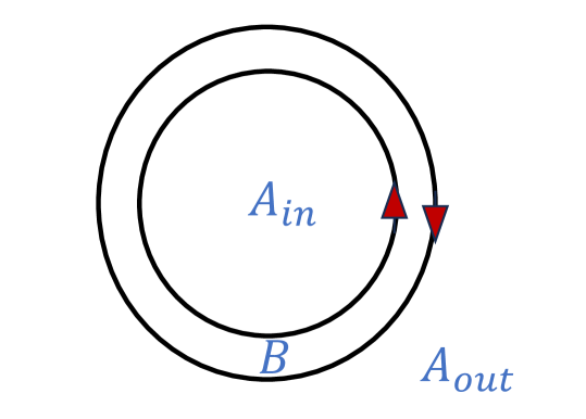
Figure 7: Tripartition $A_{in}\cup B\cup A_{out}$ of a 2d lattice with no boundary. The red arrow depicts the orientation of $\partial A_{in}$ and $\partial A_{out}$.

We prove the above statement by contradiction. Assume that there is a symmetric FDLC $\mathcal{N}$, with each layer preserving the $\Gamma=K\times G$ symmetry, s.t. $\rho^{ss}_{\text{ASPT}}=\mathcal{N}[\rho_{\text{trivial}}]$. Notably, the following discussion applies for both the case $K=\mathbb{Z}_{2}^{BC},G=\mathbb{Z}_{2}^{A}$ and $K=\mathbb{Z}_{2}^{A},G=\mathbb{Z}_{2}^{BC}$. Now take a 2D infinite lattice and take the tripartition $A_{in}\cup B\cup A_{out}$. $B$ is a finite-width strip separating the inner and outer region, and we require its width (in units of lattice spacing) to be large compared to the depth of $\mathcal{N}$. See Fig. 7. Since here both $K$ and $G$ are onsite symmetries, $\mathscr{U}(\gamma)=\mathscr{U}_{A_{in}}(\gamma)\circ\mathscr{U}_{B}(\gamma)\circ\mathscr{U}_{A_{out}}(\gamma)$.

We define $\mathcal{N}_{in}$ to be a restriction of $\mathcal{N}$ to region $A^{\prime}_{in}$ , with $A_{in}\subsetneq A^{\prime}_{in}\subsetneq A_{in}\cup B$. Thus $\rho_{\text{inter}}=\mathcal{N}_{in}[\rho_{\text{trivial}}]$ looks like $\rho^{ss}_{\text{ASPT}}$ in $A_{in}$ but remains the trivial product state in $A_{out}$. From the analysis in Section VII.2, we have

$$\mathscr{U}_{A_{in}}(\gamma)[\rho_{\text{inter}}]=\mathscr{V}_{\partial A_{in}}(\gamma)[\rho_{in}],$$ (81)

where $\partial A_{in}$ is a strip near the boundary of $A_{in}$, and $\mathscr{V}_{\partial A_{in}}$ is the symmetry action on $\partial A_{in}$, which is anomalous. In addition, $\mathscr{U}_{B}(\gamma)[\rho_{\text{inter}}]=\rho_{\text{inter}}$. Thus

$$\begin{split}\mathscr{U}(\gamma)[\rho_{\text{inter}}]&=\mathscr{V}_{\partial A_{in}}(\gamma)\circ\mathscr{U}_{B}(\gamma)[\rho_{\text{inter}}]\\ &\equiv{\mathscr{I}}(\gamma)[\rho_{\text{inter}}]=\rho_{\text{inter}}.\end{split}$$ (82)

Therefore, $\mathscr{I}(\gamma)$ is an anomalous symmetry action, supported on the 1D interface between $A_{in}$ and $A_{out}$, which means that its action is characterized by a nontrivial element in $H^{3}(\Gamma,U(1))/H^{3}(G,U(1))$. However, this contradicts Theorem 1: Since $\rho_{\text{inter}}$ is obtained from the trivial product state from $\mathcal{N}_{in}$, a symmetric FDLC, it should be anomaly free. In conclusion, such FDLC connecting $\rho_{\text{trivial}}$ to $\rho^{ss}_{\text{ASPT}}$ does not exist.

In the above, we hide some subtleties by abusing Theorem 1. Strictly speaking, since we are analyzing anomalies of the effective symmetry action on the interface, instead of the original global symmetry transformation, the validity of Theorem 1 needs to be verified in this context. We bridge this gap below. First, we can apply the same trick as in the proof of Theorem 1, i.e., purifying both the initial state $\rho_{\text{trivial}}$ and the quantum channel $\mathcal{N}_{in}$, thus arriving at a purification of $\rho_{\text{inter}}$, denoted as $|\psi_{\text{inter}}\rangle$, which should be SRE. For $|\psi_{\text{inter}}\rangle$, we can again localize the global symmetry transformation to the interface, where the effective symmetry action should be anomaly free (See Lemma 3 in Else and Nayak (2014)). It then contradicts with the anomalous symmetry action on the interface for $\rho_{\text{inter}}$, with similar reasons to our original proof of Theorem 1.

So far, we have not utilized any special properties of the two models we constructed, apart from the boundary anomaly, which we believe is a generic feature of ASPT. Thus the above argument can be applied to other ASPTs. It can also be generalized to prove the separation of mixed-state phases between two symmetric states (from the DDW construction) $\rho_{1},\rho_{2}$ with different types of boundary anomalies, with the following adjustments: First, we still assume the existence of symmetric FDLC $\mathcal{N}$, $\rho_{2}=\mathcal{N}[\rho_{1}]$ and construct $\rho_{\text{inter}}=\mathcal{N}_{in}[\rho_{1}]$. Second, apply the same type of analysis, we will get $\mathscr{U}_{A_{out}}(\gamma)[\rho_{\text{inter}}]=\mathscr{V}_{\partial A_{in}}(\gamma)\circ\mathscr{U}_{B}(\gamma)\circ\mathscr{V}_{\partial A_{out}}(\gamma)[\rho_{\text{inter}}]\equiv{\mathscr{I}}(\gamma)[\rho_{\text{inter}}]$, where the anomalous action $\mathscr{V}_{\partial A_{in}},\mathscr{V}_{\partial A_{out}}$ are characterized by different nontrivial elements $[\Omega_{1}],[\Omega_{2}]$ in $H^{3}(\Gamma,U(1))/H^{3}(G,U(1))$. Thus $\mathscr{I}(\gamma)$ is characterized by $[\Omega_{1}][\Omega_{2}]^{-1}\neq[1]$. The inverse comes from the opposite orientations of $\partial A_{in}$ and $\partial A_{out}$. Finally, note that states constructed from the DDW method become trivial when we only have weak symmetries. Therefore, we can construct a FDLC $\varepsilon$ with the weak symmetry $G$ (each layer of $\varepsilon$ is $G$-symmetric) to prepare $\rho_{1}$ from the trivial symmetric product state, so $\rho_{\text{inter}}=\mathcal{N}_{in}\circ\varepsilon[\rho_{\text{trivial}}]$, which leads to contradiction with Theorem 1.

VIII Discussion

In the end, we list some interesting future directions.

1. In this paper we only focus on symmetries of the direct product product type. In general the full symmetry group can be a group extension $1\rightarrow K\rightarrow\Gamma\rightarrow G\rightarrow 1$, where $K$ is a normal subgroup of $\Gamma$ and $G=\Gamma/K$. For example, for nontrivial group extension $\Gamma$, the so-called intrinsically mixed ASPT is constructed Ma et al. (2023), which is similar to intrinsically gapless SPT in closed systems Thorngren et al. (2021); Yang et al. (2023); Li et al. (2022b); Ma et al. (2022); Wen and Potter (2023a); Li et al. (2023); Wen and Potter (2023b). It is intriguing to work out the bulk-edge correspondence in that case.

2. Here we have only investigated anomalies of $0$-form global symmetries. It is interesting to generalize the discussion to anomalies involving higher-form symmetries Gaiotto et al. (2015). Although we do not have a systematic treatment yet, we note that many aspects of the recently investigated mixed-state topological order in decohered toric code can be understood from 1-form symmetry anomaly. Recall that the toric code model has two 1-form symmetries, $\mathbb{Z}_{2}^{(1),e}$ and $\mathbb{Z}_{2}^{(1),m}$, whose defects are $e,m$ anyons, respectively. The nontrivial mutual statistics between $e,m$ indicates a mixed anomaly between $\mathbb{Z}_{2}^{(1),e}$ and $\mathbb{Z}_{2}^{(1),m}$ Wen (2019). By adding some single-qubit phase errors (or bit-flip errors), one of the 1-form symmetries becomes a weak symmetry. Still, the remaining symmetry has strong-weak mixed anomalies, which can be easily seen using the superoperator representation. The classical memory Fan et al. (2023); Bao et al. (2023); Lee et al. (2023) and anyon braiding statistics Wang et al. (2023a); Liu (2023) can both be viewed as consequences of the anomaly. Also, a case with anomaly strong 1-form symmetry is studied in Wang et al. (2023a), where the anomaly leads to novel quantum topological order without quantum memory.

3. It is also interesting to extend the discussion to mixed anomalies between internal symmetries and spatial symmetries, e.g., translation symmetries, generalizing the Lieb-Schultz-Mattis (LSM) theorem Lieb et al. (1961); Oshikawa (2000); Hastings (2004); Fuji (2016); Watanabe et al. (2015); Huang et al. (2017); Yao et al. (2019); Thorngren and Else (2018); Yao and Oshikawa (2021); Yao et al. (2023); Cheng and Seiberg (2023b) to open quantum systems. Various versions of the LSM theorem in open quantum systems have already been proposed recently Kawabata et al. (2024); Zhou et al. (2023); Hsin et al. (2023); Zang et al. (2023); Lessa et al. (2024), but the general LSM constraint on mixed-state quantum phases remains to be uncovered.

4. Besides, the investigation of anomalous global symmetry in this paper is based on anomaly cocycle of the Else-Nayak method. Recent studies have proved that in (1+1)-D closed systems, the anomaly cocycle must be trivial to enable consistent lattice gauging Seifnashri (2023). Thus it would be interesting to further explore the understanding of anomaly in open systems and its constraint on mixed-state phases from the view of the obstruction to gauging.

5. We only briefly discuss anomalies in higher dimensions without giving examples. It is desirable to see what types of nontrivial phases with anomalies can be realized in higher dimensions, and what is the higher dimensional generalization of the anomaly-enforced boundary correlation discussed in Section V and VI.

Appendix A Boundary correlation enforced by strong-weak mixed anomalies.

In this appendix, we focus on the $(1+1)$-D open quantum systems with mixed anomalies between strong symmetry $K$ and weak symmetry $G$, and discuss its implication on the boundary correlation. As stated in Section VI, in this case it is unclear whether the conclusion in Theorem 2 still holds generally, but at least the anomaly leads to a nontrivial Renyi-2 correlation.

Theorem 4. For a $(1+1)$-D state $\rho$ with anomalous symmetry $\Gamma=K\times G$, under OBC, there must exist long-range boundary correlation for Renyi-2 correlators. $\frac{\text{Tr}(\rho O_{l}O_{r}\rho O^{\prime}_{l}O^{\prime}_{r})}{\text{Tr}(\rho^{2})}-\frac{\text{Tr}(\rho O_{l}\rho O^{\prime}_{l})}{\text{Tr}(\rho^{2})}\frac{\text{Tr}(\rho O_{r}\rho O^{\prime}_{r})}{\text{Tr}(\rho^{2})}\neq 0$.

Proof. We can repeat the steps (59),(60),(61),(62) in the proof of Theorem 2, replacing $U_{\text{OBC}},W$ with $\mathscr{U}_{\text{OBC}},\mathscr{W}$. Then, similar to the analysis below (62), we have

$$\mathscr{W}(\gamma_{1},\gamma_{2})[\rho]=\lambda(\gamma_{1})\lambda(\gamma_{2})\lambda^{-1}(\gamma_{1},\gamma_{2})\rho,$$ (83)

from the condition that $\rho$ is $\Gamma$-symmetric. On the other hand, $\exists\gamma=k\cdot g,\gamma^{\prime}=k^{\prime}\cdot g^{\prime}$, s.t.

$$\mathscr{W}_{l(r)}(\gamma,\gamma^{\prime})[\rho]\equiv W_{l(r)}(\gamma,\gamma^{\prime})\rho W_{l(r)}^{\dagger}(g,g^{\prime})\neq\beta(\gamma,\gamma^{\prime})\rho$$ (84)

for any U(1) phase factor $\beta$, which follows from the condition that $\Gamma$ is anomalous. Since the eigenvalues of $\mathscr{W}_{l(r)}(\gamma,\gamma^{\prime})$ are all distributed on the unit circle on the complex plane,

$$|\frac{\text{Tr}(\rho\mathscr{W}_{l(r)}(\gamma,\gamma^{\prime})[\rho])}{\text{Tr}(\rho^{2})}|<1.$$ (85)

Therefore,

$$\begin{split}&\frac{\text{Tr}[\rho W_{l}(\gamma,\gamma^{\prime})W_{r}(\gamma,\gamma^{\prime})\rho W_{l}(g,g^{\prime})W_{r}(g,g^{\prime}))]}{\text{Tr}(\rho^{2})}\\ -&\frac{\text{Tr}[\rho W_{l}(\gamma,\gamma^{\prime})\rho W_{l}(g,g^{\prime})]}{\text{Tr}(\rho^{2})}\frac{\text{Tr}[\rho W_{r}(\gamma,\gamma^{\prime})\rho W_{r}(g,g^{\prime})]}{\text{Tr}(\rho^{2})}\neq 0.\end{split}$$ (86)

∎

Furthermore, for onsite weak symmetry $G$, we can take $W_{l}(g)=W_{r}(g)=1$. Then (84) leads to $|\text{Tr}[W_{l(r)}(\gamma,\gamma^{\prime})\rho]|<1$. Together with (83), we get

$$\text{Tr}[W_{l}(\gamma,\gamma^{\prime})W_{r}(\gamma,\gamma^{\prime})\rho]-\text{Tr}[W_{l}(\gamma,\gamma^{\prime})\rho]\text{Tr}[W_{r}(\gamma,\gamma^{\prime})\rho]\neq 0,$$ (87)

which proves Theorem 3 in the main text by construction.

Appendix B $(1+1)$-D steady-state average SPT

In this appendix, we provide the detail of a (1+1)-D spin chain described by Lindbladians, whose steady state is (65). Under PBC, the Hamiltonian here is zero and dissipators are as follows:

$$\begin{split}&l^{1}_{2i}=\sigma^{z}_{2i}\sigma^{z}_{2i+2}\frac{1-\tau^{z}_{2i-1}\sigma^{x}_{2i}\tau^{z}_{2i+1}}{2},\\ &l^{2}_{2i-1}=\tau^{z}_{2i-1},\\ &l^{3}_{2i-1}=\sigma^{z}_{2i-2}\tau^{z}_{2i-1}\sigma^{z}_{2i},\end{split}$$ (88)

The effect of dissipators $l^{1}$ is to decorate $K$-charges $\sigma^{x}_{2i}=-1$ on $G$-domain walls. More precisely, such a term can only move or annihilate the excitation configuration $\tau^{z}_{2i-1}\sigma^{x}_{2i}\tau^{z}_{2i+1}=-1$. The effect of $l^{2}$ is to dephase the $\tau$ spins and to select diagonal domain wall configurations. The effect of $l^{3}$ is to incoherently proliferate the $G$ domain wall configurations. As mentioned in Sec. VII.1, $U(\text{CZ})$ can relate this ASPT model and a Lindbladians :

$$\begin{split}&l^{1}_{2i}=\sigma^{z}_{2i}\sigma^{z}_{2i+2}\frac{1-\sigma^{x}_{2i}}{2},\\ &l^{2}_{2i-1}=\tau^{z}_{2i-1},\quad l^{3}_{2i-1}=\tau^{x}_{2i-1}.\end{split}$$ (89)

The latter has the trivial mixed state $\rho_{\text{trivial}}=\rho_{\sigma}^{\rightarrow}\otimes I_{\tau}$. Thus the Lindbladian with dissipators (88) has the steady state (65). Such steady state has the string order $\text{Tr}(\tau^{z}_{2j-1}(\prod^{k}_{i=j}\sigma^{x}_{2i})\tau^{z}_{2k+1}\rho_{\text{cluster}})=1$.

As the nontrivial boundary modes protected by the global symmetry is a signature of pure-state SPT, we find that the same is true for the average SPT in Lindbladians, which also comes from an anomaly on the boundary. We place the spin system on an open chain with length $L\in 2\mathbb{Z}$. Similarly, we focus on the subspace

$$\mathcal{C}=\{\rho_{j}:\mathcal{L}_{\text{bulk}}[\rho_{j}]=0\}.$$ (90)

Here $\mathcal{L}_{\text{bulk}}$ is defined by only keeping terms fully supported on the open chain in (88), so $\mathcal{C}$ can be viewed as the space where edge modes live. By using $U(\text{CZ})$, which is now truncated at the edge, we can identify that $\mathcal{C}$ is a 4-dimensional space satisfying $\tau^{z}_{2i-1}\sigma^{x}_{2i}\tau^{z}_{2i+1}\rho_{j}=\rho_{j}$ and $\sigma^{z}_{2i}\tau^{x}_{2i+1}\sigma^{z}_{2i+2}\rho_{j}\sigma^{z}_{2i}\tau^{x}_{2i+1}\sigma^{z}_{2i+2}=\rho_{j}$ where $1\leq i\leq L/2-1$. Moreover, the Pauli operators, which preserve $\mathcal{C}$, are given by the following dressed edge operator

$$\tilde{\tau}^{\alpha}_{1}=U(\text{CZ})\tau^{\alpha}_{1}U(\text{CZ}),\quad\tilde{\sigma}^{\alpha}_{L}=U(\text{CZ})\sigma^{\alpha}_{L}U(\text{CZ})$$ (91)

where $\alpha=x,y,z$ Following the same method in sec.VII.2, we can show the symmetry operator fractionalizes as $U_{K/G}\tilde{\tau}^{\alpha}_{1}U_{K/G}=L_{K/G}\tilde{\tau}^{\alpha}_{1}L_{K/G},\quad U_{K/G}\tilde{\sigma}^{\alpha}_{L}U_{K/G}=R_{K/G}\tilde{\sigma}^{\alpha}_{L}\mathcal{R}_{K/G}$, where

$$\begin{split}&L_{K}=\tilde{\tau}^{z}_{1}=\tau^{z}_{1},R_{K}=\tilde{\sigma}^{x}_{L}=\tau^{z}_{L-1}\sigma^{x}_{L},\\ &L_{G}=\tilde{\tau}^{x}_{1}=\tau^{x}_{1}\sigma^{z}_{2},R_{G}=\tilde{\sigma}^{z}_{L}=\sigma^{z}_{L}.\end{split}$$ (92)

Thus the symmetry action on the edge modes ($\rho_{j}\in\mathcal{C}$) reads:

$$\begin{split}\mathscr{U}_{K/G}&=\mathscr{L}_{K/G}\circ\mathscr{R}_{K/G},\\ \mathscr{L}_{K}[\rho_{j}]&\equiv L_{K}\rho_{j},\mathscr{R}_{K}[\rho_{j}]\equiv R_{K}\rho_{j},\\ \mathscr{L}_{G}[\rho_{j}]&\equiv L_{G}\rho_{j}L^{\dagger}_{G},\mathscr{R}_{G}[\rho_{j}]\equiv R_{G}\rho_{j}R^{\dagger}_{G}\end{split}$$ (93)

Thus the effective symmetry forms a projective representation on each edge, $\mathscr{L}_{K}\circ\mathscr{L}_{G}=-\mathscr{L}_{G}\circ\mathscr{L}_{K}$, and similarly for $\mathscr{R}$. As in pure state, the nontrivial projective representation can be defined as an anomaly in (0+1) dimension. of $\mathcal{L}$ and $\mathcal{R}$ gives rise to at least 2-dimensional edge modes at each boundary.

Appendix C $(2+1)$-D steady-state average SPT with $K=\mathbb{Z}^{B}_{2}\times\mathbb{Z}^{C}_{2}$ and $G=\mathbb{Z}^{A}_{2}$

In this appendix, we will study the Lindbladians (80), mainly on the SPT feature of steady state and the anomalous symmetry of edge theory.

At first, the SPT feature can be detected by adding a $\mathbb{Z}^{A}_{2}$ domain wall on a loop $N_{A}$ in the dual lattice of $A$ sublattice, i.e., $B$ and $C$ sublattice. This domain wall is realized by conjugating the steady state by $\prod_{i\in M_{A}}\sigma^{x}_{i}$, where $M_{A}$ only involves the $A$ sites enclosed by $N_{A}$. Then we have

$$\begin{split}\prod_{M_{A}}\sigma^{x}_{i}\rho^{ss}_{\text{ASPT}}\prod_{M_{A}}\sigma^{x}_{i}=U_{N_{A}}(\text{CZ})\rho^{ss}_{\text{ASPT}}U^{\dagger}_{N_{A}}(\text{CZ}).\end{split}$$ (94)

The $U_{N_{A}}(\text{CZ})$ is known to stack a $(1+1)$-D $\mathbb{Z}_{2}\times\mathbb{Z}_{2}$ SPT on $N_{A}$ in closed systems. Moreover, we can further add a strong $\mathbb{Z}^{B}_{2}$ domain wall on $N_{B}$, which is realized by applying $\prod_{i\in M_{B}}\tau^{x}_{i}$ on the left of the steady state. By the same proof as Eq. (71) and Eq. (73), we have

$$\begin{split}&\prod_{M_{A}}\sigma^{x}_{i}\prod_{M_{B}}\tau^{x}_{j}\rho^{ss}_{\text{ASPT}}\prod_{M_{B}}\tau^{x}_{j}\\ =&\prod_{N_{A}\cap N_{B}}(\mu^{z}_{i})^{s_{i}}U_{N_{A}\cup N_{B}}(\text{CZ})\rho^{ss}_{\text{ASPT}}\prod_{M_{B}}\tau^{x}_{j}.\end{split}$$ (95)

Here $s_{i}$ is the number of 1-links of $C$ vertex $i$ whose endpoints are in $M_{B}$ and $M_{A}$. This shows the codimension-2 defect, i.e., intersection points of $\mathbb{Z}^{A}_{2}$ and $\mathbb{Z}^{B}_{2}$ domain walls with odd $s_{i}$ are decorated with $\mathbb{Z}^{C}_{2}$ charge.

Indeed, this model also realizes an ASPT when we only consider strong $\mathbb{Z}^{BC}_{2}$ symmetry and weak $\mathbb{Z}^{A}_{2}$ symmetry. This statement can be seen from the corresponding group cohomology and boundary anomaly as follows. Let us consider a typical cocycle $\omega(\gamma_{1},\gamma_{2},\gamma_{3})=(-1)^{b_{1}c_{2}a_{3}}$ belonging to nontrivial class of $H^{1}(\mathbb{Z}^{A}_{2},H^{2}(\mathbb{Z}^{B}_{2}\times\mathbb{Z}^{C}_{2},U(1))$, where $\gamma_{i}=(a_{i},b_{i},c_{i})\in\mathbb{Z}^{A}_{2}\times\mathbb{Z}^{B}_{2}\times\mathbb{Z}^{C}_{2}$ and $a,b,c=0,1$ represent trivial and nontrivial elements, respectively. Then one can directly calculate the gauge invariant combinations:

$$\begin{split}&\omega(A,BC,BC)\omega(ABC,A,BC)\omega(ABC,ABC,A)\omega(A,I,A)\\ &=1\times 1\times(-1)\times 1=-1,\\ &\omega(BC,BC,BC)\omega(BC,I,BC)=1\times 1=1,\end{split}$$ (96)

where $A=(1,0,0),BC=(0,1,1)$. The first combination and second combination classify $H^{2}(\mathbb{Z}^{A}_{2},H^{1}(\mathbb{Z}^{BC}_{2},U(1))$ and $H^{3}(\mathbb{Z}^{BC}_{2},U(1))$. Thus this result implies that the cocycle of $\mathbb{Z}^{A}_{2}$ and $\mathbb{Z}^{BC}_{2}$ symmetry of this ASPT belongs to nontrivial class of $H^{2}(\mathbb{Z}^{A}_{2},H^{1}(\mathbb{Z}^{BC}_{2},U(1))$.

Moreover, we can also study how the global symmetry acts on the edge DOFs on an open lattice in Fig. 6. We consider Lindblad $\mathcal{L}=\mathcal{L}_{\text{bulk}}+\mathcal{L}_{\text{edge}}$ and focus on the subspace $\mathcal{C^{\prime}}$ which involves steady states of $\mathcal{L}_{\text{bulk}}$:

$$\mathcal{C^{\prime}}=\{\rho_{j}:\mathcal{L}_{\text{bulk}}[\rho_{j}]=0\}.$$ (97)

By conjugating $U(\text{CCZ})$, which is truncated at the edge, the bulk and edge DOFs are decoupled. In the bulk, there is only a single steady state $\rho^{ss}_{\tau,\mu}=|\rightarrow\rightarrow\cdots\rightarrow\rangle\langle\rightarrow\rightarrow\cdots\rightarrow|$ with $\prod_{i,j\in\text{bulk}}\tau^{x}_{i}\mu^{x}_{j}=1$ and $\rho^{ss}_{\sigma}=I_{\sigma}$. It is easy to check that the dressed edge operators (75) also preserve $\mathcal{C^{\prime}}$ and compose a complete set of Pauli operators for edge DOFs in $\mathcal{C^{\prime}}$. Due to (76), strong $U_{B}U_{C}$ and weak $U_{A}$ symmetry will restrict to strong $\prod_{i,j\in\text{edge}}\tilde{\tau}^{x}_{i}\tilde{\mu}^{x}_{j}$ and weak $\tilde{U}(\text{CZ})$ symmetry on the edge DOFs, which is same as Example 3 in section V. Since the strong $\prod_{i,j\in\text{edge}}\tilde{\tau}^{x}_{i}\tilde{\mu}^{x}_{j}$ and weak $\tilde{U}(\text{CZ})$ has the mixed anomaly, the bulk model (80) should realize a $\mathbb{Z}^{BC}_{2}\times\mathbb{Z}^{A}_{2}$ ASPT.