FHAUC: Privacy Preserving AUC Calculation for
Federated Learning using Fully Homomorphic Encryption

Abstract

Ensuring data privacy is a significant challenge for machine learning applications, not only during model training but also during evaluation. Federated learning has gained significant research interest in recent years as a result. Current research on federated learning primarily focuses on preserving privacy during the training phase. However, model evaluation has not been adequately addressed, despite the potential for significant privacy leaks during this phase as well. In this paper, we demonstrate that the state-of-the-art AUC computation method for federated learning systems, which utilizes differential privacy, still leaks sensitive information about the test data while also requiring a trusted central entity to perform the computations. More importantly, we show that the performance of this method becomes completely unusable as the data size decreases. In this context, we propose an efficient, accurate, robust, and more secure evaluation algorithm capable of computing the AUC in horizontal federated learning systems. Our approach not only enhances security compared to the current state-of-the-art but also surpasses the state-of-the-art AUC computation method in both approximation performance and computational robustness, as demonstrated by experimental results. To illustrate, our approach can efficiently calculate the AUC of a federated learning system involving $100$ parties, achieving 99.93% accuracy in just 0.68 seconds, regardless of data size, while providing complete data privacy.

1 Introduction

Today, machine learning has become a powerful tool that can be applied to a myriad of fields. However, with concerns about data privacy and confidentiality getting more and more attention from governments around the world, and with regulations like GDPR and CCPA to regulate how personal data can be managed, privacy-preserving machine learning techniques like Federated learning (FL) received tremendous research interest (Li et al., 2020; Bonawitz et al., 2019; Mothukuri et al., 2021).

FL is defined as a setting where multiple input parties, collectively train a machine learning model, often through a central server (e.g. service provider, aggregator), while keeping their local data private (Kairouz et al., 2021). Although the term FL was first proposed with applications for mobile and edge devices in mind (McMahan et al., 2017; McMahan & Ramage, 2017), the significance of utilizing FL in other fields has vastly increased, which include less number of more reliable participants such as collaborating organizations (Kairouz et al., 2021). Data partition between the input parties plays an important role in the operation of the FL system. Based on how the data is partitioned across participants, FL is defined in two categories: Horizontal and Vertical Federated Learning. In this paper, our focus is on Horizontal FL, where each data sample is divided among input parties, such as data from individual patients.

Current research on the privacy of FL systems mostly focuses on the training phase, where the model architecture or parameters are communicated between the participants or the aggregator (Zhao et al., 2020; Zhu et al., 2019; Wei et al., 2020). After the training phase is completed, the input parties also need to test the performance of the model on test data. Although input parties with abundant test samples available can test the performance of the global model on their own, parties with a limited number of samples greatly benefit from collaborative performance evaluation. However, since private data is used for testing these models, privacy leakage can also occur during the model evaluation phase (Stoddard et al., 2014; Matthews & Harel, 2013). Therefore, we require a privacy-preserving solution for collaborative model performance evaluation in FL systems.

The current state-of-the-art method for privacy-preserving model performance evaluation in FL systems utilizes differential privacy (DP) (Sun et al., 2022) to compute the area under the Receiver Operating Characteristics (ROC) curve. The ROC curve is an effective way to assess the performance of a machine learning model on a binary classification problem, and the area under the ROC curve (AUC) provides a summary of the ROC curve. While differential privacy can preserve the privacy of individual samples, it fails to prevent a semi-honest aggregator from inferring sensitive information about the local data, local AUC scores of participants, and the performance of the global model. Additionally, this method requires a trusted central entity, offering no security against malicious adversaries capable of tampering with the data. Finally, the results of our experiments reveal that as the size of the global test data decreases, the AUC values computed by this method become completely unreliable and unusable.

In this context, we propose that Fully Homomorphic Encryption (FHE) can be utilized instead of DP-based techniques. FHE, a cryptographic primitive enabling computations on ciphertexts without decryption, is a state-of-the-art privacy-preserving computation technique that has seen great research interest in FL applications (Fang & Qian, 2021; Zhang et al., 2020). Previous research has only used FHE to protect privacy during the training phase of federated FL systems. In this work, we extend the use of FHE to preserve privacy during model performance evaluation. To achieve this goal, we propose an efficient, accurate, robust, and more secure method of calculating the AUC in Horizontal FL systems using FHE, which is secure against both semi-honest and malicious adversaries. To the best of our knowledge, FHAUC is the first method to utilize FHE for privacy-preserving model evaluation in Horizontal FL systems while providing security against both semi-honest and malicious adversaries. Our contributions are as follows:

1. While current research in FL predominantly centers around improving model training, there exists a notable gap in the literature addressing the evaluation of global model performance on distributed test data. Additionally, through empirical results, we show that the current state-of-the-art DP-based AUC computation method faces significant limitations, rendering it impractical for scenarios involving a small global dataset and posing potential risks of leaking sensitive information from the local data of input parties.

2. Therefore, we introduce a novel method that utilizes FHE to efficiently and accurately compute AUC in Horizontal FL systems while also ensuring complete data privacy and security. This includes protection against not only a semi-honest aggregator but also a malicious aggregator, as proven in our security analysis, which has not been addressed in the literature before.

3. The results of our experiments show that our AUC computation method can compute highly accurate AUC values when compared to ground truth, regardless of global data size. Our method outperforms the state-of-the-art DP-based AUC computation method in terms of both approximation performance and data privacy.

4. Although our approach employs FHE, our results demonstrate that the computation time remains well within real-time use, even when executed on a single core. Notably, the efficiency of our method is independent of the global data size, showcasing its scalability and practical applicability.

2 Preliminaries

In this section, we present some background information on the concepts used throughout the paper.

2.1 ROC curve and AUC

Conventional AUC computation requires True Positive Rate (TPR) and False Positive Rate (FPR) values to compute the AUC. However, obtaining either of these values presents a challenge when computing the AUC through FHE due to the difficulty of performing division in FHE schemes. To minimize the number of division operations, the formula we employed to compute the AUC is as follows:

$$\footnotesize AUC=\frac{\sum_{i=1}^{\mathcal{D}}(TP^{i}+TP^{i-1})\cdot(FP^{i}-FP^{i-1})}{2\cdot TP^{\mathcal{D}}\cdot FP^{\mathcal{D}}}$$ (1)

We note that the formula utilizes TP and FP values to compute the AUC. Hence, we reduce the number of division operations required to compute the AUC to one, a property we exploit to compute the AUC while leveraging FHE. Further information is provided in Section A of the Appendix.

2.2 Trapezoidal Rule

The trapezoidal rule approximates definite integrals or areas under curves (Yeh et al., 2002). It divides the curve into sub-intervals, forming trapezoids under the curve, and calculates their areas, summing them for an approximate area under the curve. The formula for approximating the area under the ROC curve resembles Equation 1. If $S_{N}$ denotes the set of decision points partitioning $[0,1]$, we use $N$ decision points instead of threshold samples, as follows, where $N$ represents the set size of $S_{N}$:

$$\footnotesize AUC\approx\sum_{n=1}^{N-1}\frac{(TP^{n}+TP^{n-1})\cdot(FP^{n}-FP^{n-1})}{2\cdot TP^{N-1}\cdot FP^{N-1}}$$ (2)

where, similar to Equation 1, the $TP^{N-1}$ and $FP^{N-1}$ values in the denominator represent the total number of positive and negative samples, respectively. Our proposed AUC computation method uses the trapezoidal rule to calculate the approximate AUC of a global federated learning model while maintaining privacy by leveraging FHE.

2.3 Homomorphic Encryption

Homomorphic encryption (HE) enables operations on encrypted data, producing results mirroring those of operations on plaintexts. Additive HE schemes, like the Paillier scheme (Paillier, 1999), support addition over encrypted data, while schemes such as RSA (Rivest et al., 1978) and ElGamal (ElGamal, 1985) facilitate multiplication, falling under multiplicative HE schemes. Partial HE schemes support only one operation—either addition or multiplication. Fully Homomorphic Encryption (FHE) schemes, first introduced by Gentry (Gentry, 2009) using lattice theory, support both operations. FHE encompasses various schemes categorized by supported data types, with noise introduced during encryption and key generation.

For privacy-preserving AUC computation, we employ the Cheon-Kim-Kim-Song (CKKS) scheme (Cheon et al., 2017), allowing approximate computations over real or complex number vectors. We evaluate our method using OpenFHE, an open-source Fully Homomorphic Encryption library (Al Badawi et al., 2022).

3 Related Work

Most research on FL systems is focused on privacy preservation during the training phase (Zhao et al., 2020; Zhu et al., 2019; Wei et al., 2020; Sav et al., 2022) with very few methods proposed for privacy preservation during the model evaluation phase (Ünal et al., 2023; Sun et al., 2022).

Multi-Party Computation. A multi-party computation based approach for calculating the exact AUC within a system having multiple data sources is proposed by (Ünal et al., 2023). Although the proposed method is capable of computing the ground truth AUC, the use of privacy-preserving merge sort results in infeasible computation times. The experimental results presented by (Ünal et al., 2023) show that the proposed method takes approximately 1400 seconds to compute the AUC on just 8000 global data samples with 8 parties. However, our approach can compute the approximate AUC with near-perfect accuracy while providing the same level of security in just a few seconds.

Differential Privacy. The most notable and state-of-the-art method, DPAUC${}_{\text{Lap}}$, proposed by (Sun et al., 2022), utilizes differential privacy for privacy-preserving AUC computation in FL systems. DPAUC${}_{\text{Lap}}$, which we will henceforth refer to as DPAUC, utilizes Laplacian noise to achieve differential privacy, while using Trapezoidal Rule to approximate the AUC value. While the experimental results presented demonstrate that DPAUC can produce accurate AUC calculations, (Sun et al., 2022) do not assess the performance of DPAUC with different amounts of global test data. The experiments were conducted on a large test dataset consisting of $458407$ samples, minimizing the impact of noise addition on the accuracy of the approximations. However, our own experiments in Section 5 reveal that DPAUC yields completely unusable AUC computations when the global data size is small. Low amounts of test data are prevalent in many fields, particularly in the medical domain (Kononenko, 2001; Foster et al., 2014), which is a major application area for FL systems. Furthermore, while DPAUC achieves differential privacy through the addition of noise, it still inadvertently discloses sensitive information regarding the local data of each participant and the performance of the global and local models within the FL system. Detailed attack scenario and empirical results revealing the information leakage in DPAUC are provided in Section B of the Appendix.

4 Method

This section first outlines our threat model and then details our approaches for computing AUC in an FL system in the presence of both the semi-honest aggregator and the malicious aggregator.

4.1 Notations

For the rest of the paper, we represent the number of input parties as $S_{M}$ whose size is $M$. We denote the set of threshold samples as $S_{N}$ whose size is represented as $N$. $TP^{n}_{m}$ and $FP^{n}_{m}$ represent the number of true positives and false positives of input party $m$ on decision point $n$, respectively. Except $n=N-1$ in malicious FHAUC, $T^{n}_{m}$ denotes $(TP^{n}_{m}+TP^{n-1}_{m})$ and $F^{n}_{m}$ denotes $(FP^{n}_{m}-FP^{n-1}_{m})$. Moreover, in malicious FHAUC, these values are masked by some random values. $X_{m}$ represents the dataset of the input party $m$.

4.2 Threat Model

Our focus lies in the performance analysis phase within a Horizontal FL environment. Consequently, we assume that the model training is conducted securely. The environment comprises multiple input parties (such as devices, hospitals) and a central non-input party (like an aggregator, server) responsible for computing the AUC. We assume the input parties to be semi-honest and the aggregator to be semi-honest or malicious. Semi-honest adversaries strictly adhere to the computation algorithm but possess curiosity to extract as much information as possible, while malicious adversaries can arbitrarily deviate from the protocol description. We assume there is no collusion between the input parties and the aggregator, ensuring the secure storage of the private key by the input parties, thereby preventing any susceptibility to leakage. Each participant possesses a shared seed used to generate cryptographically secure random numbers via AES.

4.3 Semi-honest FHAUC

In this section, we introduce our solution for computing AUC in a privacy-preserving way when dealing with semi-honest input parties and a semi-honest aggregator, termed as semi-honest FHAUC. We will initially give the details of the setup phase of the semi-honest FHAUC.

4.3.1 Setup

FHAUC relies on secure key distribution through a public key infrastructure, where the private key of FHE $K$ is distributed to each party within the FL system. The process begins with the aggregator randomly selecting an input party within the FL system to generate the key pair required for the AUC computation. The selected party shares the public key with the aggregator, which is necessary for performing FHE operations on the ciphertexts, and distributes the private key among other input parties using public-key encryption. The public keys of the input parties can be obtained through a trusted third party, such as a certificate authority. The use of a trusted third party for private key distribution is a widely adopted practice in various solutions that employ FHE (Liu et al., 2019; Zhang et al., 2020). While our primary focus lies in ensuring the privacy and security of the computation phase, it is important to note that the security of the key distribution phase is not within the scope of our paper. The issue of secure key distribution within a distributed environment often stands as an independent challenge, and it similarly falls beyond the scope of the existing FHE-based solutions outlined in the literature (Liu et al., 2019; Zhang et al., 2020; Aono et al., 2017).

The decision points $S_{N}$ to be used for the approximate AUC computation can be pre-determined among the participants or agreed upon by the randomly selected input party during the setup phase. In the latter case, the agreed-upon $S_{N}$ can be distributed to each party along with the private key. The choice of decision points can also be made public since the public availability of $S_{N}$ does not compromise the privacy of FHAUC.

4.3.2 Secure Computation

After the completion of the setup phase, both the input parties and the aggregator proceed with the AUC computation. The workflow of our method is shown in Figure 1. The algorithm consists of eight steps:

1. Each input party calculates their prediction confidence scores $\Phi_{m}=f(X_{m})$ by using the global model $f$ on their respective local data $X_{m}$.

2. For each decision threshold $n\in\{0,\ldots,(N-1)\}$, each input party $m$ computes the TP${}^{n}_{m}$, and FP${}^{n}_{m}$ statistics based on their local data. TP${}^{N-1}_{m}$ denotes the total number of positively labeled samples and FP${}^{N-1}_{m}$ denotes the total number of negatively labeled samples within $X_{m}$.

3. Each input party $m\in\{0,\ldots,(M-1)\}$ computes $T^{n-1}_{m}=TP^{n}_{m}+TP^{n-1}_{m}$ and $F^{n-1}_{m}=FP^{n}_{m}-FP^{n-1}_{m}$ where $n\in\{1,\ldots,(N-1)\}$.

4. Each input party $m\in\{0,\ldots,(M-1)\}$ encrypts their statistics using the FHE private key as follows: $E_{K}(\text{T}^{n-1}_{m})$ and $E_{K}(\text{F}^{n-1}_{m})$ for each $n\in\{1,\ldots,(N-1)\}$, and $E_{K}(\text{TP}^{N-1}_{m})$ and $E_{K}(\text{FP}^{N-1}_{m})$. These encrypted statistics are then sent to the aggregator.

5. The aggregator utilizes FHE to aggregate all the encrypted $\text{T}^{n-1}_{m}$ and $\text{F}^{n-1}_{m}$ of input parties to obtain $E_{K}(\text{T}^{n-1})$ and $E_{K}(\text{F}^{n-1})$ for each $n\in\{1,\ldots,(N-1)\}$.

6. The aggregator utilizes FHE to aggregate all the encrypted $\text{TP}^{N-1}_{m}$ and $\text{FP}^{N-1}_{m}$ of input parties to obtain $E_{K}(\text{TP}^{N-1})$ and $E_{K}(\text{FP}^{N-1})$.

7. The aggregator utilizes FHE to compute $E_{K}(\text{num})=E_{K}(\sum_{n=1}^{N-1}\text{T}^{n-1}\cdot\text{F}^{n-1})$ and $E_{K}(\text{denom})=E_{K}(\text{TP}^{N-1}\cdot\text{FP}^{N-1})$.

8. Aggregator generates two cryptographically secure random floating-point values $c$ and $d$, and uses them to compute $E_{K}(num\cdot d+denom\cdot c)$ and $E_{K}(denom\cdot d)$. It then sends these computed ciphertexts to the input parties along with $\frac{c}{d}$.

9. Each input party decrypts the encrypted ciphertexts to obtain $D_{K}(E_{K}(num\cdot d+denom\cdot c))=num^{\prime}$ and $D_{K}(E_{K}(denom\cdot d))=denom^{\prime}$. They then compute $\frac{num^{\prime}}{denom^{\prime}}-\frac{c}{d}=\frac{num}{denom}\approx AUC$, resulting in an approximation of the exact global AUC value.

Figure 1: The Workflow of semi-honest FHAUC.

4.4 Malicious FHAUC

In this section, we introduce our solution for privacy-preserving AUC computation in the presence of semi-honest input parties and a malicious aggregator, termed as malicious FHAUC.

The FHE schemes enable computation on encrypted data without disclosing the actual data. However, they lack mechanisms to guarantee the accuracy of computations executed by the server. This absence of computational integrity poses a risk for malicious actors to compromise security and privacy without being detected. This could result in incorrect computation results being accepted, potentially leading to unintended information exposure upon decryption (Viand et al., 2023). Detecting such malicious activities usually involves recomputing the function on plaintexts, but in settings like FL, sharing raw data with other parties isn’t feasible due to privacy regulations.

In the malicious FHAUC protocol, each input party randomizes all values of $T$ and $F$, encrypts these randomized values using the private key, and transmits the encrypted values to the aggregator. Both the random generation stage in the setup phase and the entire secure computation phase are performed twice between input parties and the aggregator. For the first computation task, the aggregator computes $(r_{0}\cdot\text{num}+r_{1}\cdot\text{denom},r_{2}\cdot\text{denom})$, and for the second computation task, it computes $(r_{0}^{\prime}\cdot\text{num}+r_{1}^{\prime}\cdot\text{denom},r_{2}^{\prime}\cdot\text{denom})$. Here, $r_{0}$, $r_{1}$, $r_{2}$, $r_{0}^{\prime}$, $r_{1}^{\prime}$, and $r_{2}^{\prime}$ are random values known only by the input parties. Ultimately, each input party extracts the AUC from $\frac{r_{0}\cdot\text{num}+r_{1}\cdot\text{denom}}{r_{2}\cdot\text{denom}}$ and AUC^′ from $\frac{r_{0}^{\prime}\cdot\text{num}+r_{1}^{\prime}\cdot\text{denom}}{r_{2}^{\prime}\cdot\text{denom}}$. If these results match, it indicates that the AUC computation followed the protocol description. Any deviation by the aggregator from the protocol description would result in this equality check failing.

The following sections outline the setup and secure computation phases of malicious FHAUC:

4.4.1 Setup

The setup phase of malicious FHAUC begins similarly to semi-honest FHAUC. It proceeds with input parties generating common random values $r_{3},r_{4},r_{5},r_{6},r_{7},r_{8}$ and two arrays, $tr^{n}_{m}$ and $fr^{n}_{m}$, consisting of random values of size $(N+1)MS$, where $r_{0}=r_{3}r_{4}$, $r_{1}=r_{5}r_{6}$, $r_{2}=r_{7}r_{8}$, $n\in\{0,\ldots,N\}$, $m\in\{0,\ldots,(M-1)\}$ and $S$ is the split count. The input parties generate a common random permutation $\pi$ of size $S(N+1)$ and an array of common random bits $b$ of size $(N+1)$.

4.4.2 Secure Computation

The steps of the secure computation performed by the aggregator in malicious FHAUC are outlined as follows. To summarize, steps 1-8 are performed by the input parties, steps 9-11 are carried out by the malicious aggregator, and step 12 is performed by the input parties. The steps of the algorithm are as follows:

1. Each input party calculates their prediction confidence scores $\Phi_{m}=f(X_{m})$ by using the global model $f$ on their respective local data $X_{m}$.

2. For each decision threshold $n\in\{0,\ldots,N-1\}$, each input party $m\in\{0,\ldots,M-1\}$ computes the TP${}^{n}_{m}$, and FP${}^{n}_{m}$ statistics based on their local data.

3. Each input party $m\in\{0,\ldots,M-2\}$ computes:

$$T^{n-1}_{m} =r_{3}(TP^{n}_{m}+TP^{n-1}_{m}+tr^{n-1}_{m})$$

$$F^{n-1}_{m} =r_{4}(FP^{n}_{m}-FP^{n-1}_{m}+fr^{n-1}_{m})$$

and the input party $M-1$ computes:

$$T^{n-1}_{M-1} =r_{3}(TP^{n}_{M-1}+TP^{n-1}_{M-1}-(tr^{n}_{0}+...+tr^{n}_{M-2}))$$

$$F^{n-1}_{M-1} =r_{4}(FP^{n}_{M-1}-FP^{n-1}_{M-1}-(fr^{n}_{0}+...+fr^{n}_{M-2}))$$

where $n\in\{1,\ldots,(N-1)\}$.

4. Each input party $m\in\{0,\ldots,M-2\}$ computes

$$T^{N-1}_{m} =r_{5}(TP^{N-1}_{m}+tr^{N-1}_{m})$$

$$F^{N-1}_{m} =r_{6}(FP^{N-1}_{m}+fr^{N-1}_{m})$$

and the input party $M-1$ computes

$$T^{N-1}_{M-1} =r_{5}(TP^{N-1}_{M-1}-(tr^{N-1}_{0}+...+tr^{N-1}_{M-2}))$$

$$F^{N-1}_{M-1} =r_{6}(FP^{N-1}_{M-1}-(fr^{N-1}_{0}+...+fr^{N-1}_{M-2}))$$

5. Each input party $m\in\{0,\ldots,M-2\}$ computes

$$DT_{m} =r_{7}(TP^{N-1}_{m}+tr^{N}_{m})$$

$$DF_{m} =r_{8}(FP^{N-1}_{m}+fr^{N}_{m})$$

and the input party $M-1$ computes

$$DT_{M-1} =r_{7}(TP^{N-1}_{M-1}-(tr^{N}_{0}+tr^{N}_{1}+...+tr^{N}_{M-2}))$$

$$DF_{M-1} =r_{8}(FP^{N-1}_{M-1}-(fr^{N}_{0}+fr^{N}_{1}+...+fr^{N}_{M-2}))$$

6. Each input party $m\in\{0,\ldots,M-1\}$ divides $T^{n}_{m}$ or $F^{n}_{m}$ into $s$ additive shares based on a common random bit $b[n]$. If $b[n]$ is $0$, the input party divides $T^{n}_{m}$ into $s$ additive shares such that $(T^{n}_{m}[0]+T^{n}_{m}[1]+...+T^{n}_{m}[S-1]=T^{n}_{m})$, while $F^{n}_{m}[s]=F^{n}_{m}$ for each $s\in\{0,\ldots,(S-1)\}$ where $n\in\{0,\ldots,(N-1)\}$. If $b[n]$ is $1$, the process is reversed.

7. Each input party permutes $T_{m}$ and $F_{m}$ with the common permutation $\pi$.

8. Each input party $m\in\{0,\ldots,M-1\}$ encrypts their statistics using the FHE private key as follows: $E_{K}(\text{T}^{n}_{m}[s])$, $E_{K}(\text{F}^{n}_{m}[s])$, $E_{K}(\text{DT}_{m})$, and $E_{K}(\text{DF}_{m})$ where $n\in\{0,\ldots,(N-1)\}$ and $s\in\{0,\ldots,(S-1)\}$. These encrypted statistics are then sent to the aggregator.

9. For each $n\in\{0,\ldots,(N-1)\}$ and $s\in\{0,\ldots,(S-1)\}$, the aggregator utilizes FHE to compute:

$$\small E_{K}(\text{T}^{n}[s]) =E_{K}(\textstyle\sum_{m=0}^{M-1}\text{T}^{n}_{m}[s])$$

$$E_{K}(\text{F}^{n}[s]) =E_{K}(\textstyle\sum_{m=0}^{M-1}\text{F}^{n}_{m}[s])$$

$$E_{K}(\text{DT}) =E_{K}(\textstyle\sum_{m=0}^{M-1}\text{DT}_{m})$$

$$E_{K}(\text{DF}) =E_{K}(\textstyle\sum_{m=0}^{M-1}\text{DF}_{m})$$

10. The aggregator utilizes FHE to compute

$$E_{K}(\sum_{n=0}^{N}\sum_{s=0}^{S-1}\text{T}^{n}[s]\cdot\text{F}^{n}[s])=E_{K}(r_{3}\cdot r_{4}\cdot\text{num}+r_{5}\cdot r_{6}\cdot\text{denom})\\ \hskip 91.04872pt=E_{K}(r_{0}\cdot\text{num}+r_{1}\cdot\text{denom})\\ \\ E_{K}(\text{DT}\cdot\text{DF})=E_{K}(r_{7}\cdot r_{8}\cdot\text{denom})=E_{K}(r_{2}\cdot\text{denom})$$

11. Aggregator generates two cryptographically secure random floating-point values $c$ and $d$, and uses them to compute $E_{K}(d\cdot(r_{0}\cdot\text{num}+r_{1}\cdot\text{denom})+c\cdot r_{2}\cdot\text{denom})$ and $E_{K}(d\cdot r_{2}\cdot\text{denom})$. It then sends these computed ciphertexts to the input parties along with $\frac{c}{d}$.

12. Each input party decrypts the encrypted ciphertexts to obtain $(d\cdot(r_{0}\cdot\text{num}+r_{1}\cdot\text{denom})+c\cdot r_{2}\cdot\text{denom})$ and $(d\cdot r_{2}\cdot\text{denom})$.

4.4.3 Verification

The random generation phase of the setup and the entire secure computation phase takes place between the input parties and the aggregator two times, using the same inputs. Subsequently, the input parties possessing the outputs of two secure computations proceed with the following verification process.

$$\text{AUC}= (\frac{d\cdot(r_{0}\cdot\text{num}+r_{1}\cdot\text{denom})+c\cdot r_{2}\cdot\text{denom}}{d\cdot r_{2}\cdot\text{denom}}$$

$$-\frac{c}{d}-\frac{r_{1}}{r_{2}})\cdot\frac{r_{2}}{r_{0}}=\frac{\text{num}}{\text{denom}}$$

$$\text{AUC}^{\prime}= (\frac{d^{\prime}\cdot(r_{0}^{\prime}\cdot\text{num}+r_{1}^{\prime}\cdot\text{denom})+c^{\prime}\cdot r_{2}^{\prime}\cdot\text{denom}}{d^{\prime}\cdot r_{2}^{\prime}\cdot\text{denom}}$$

$$-\frac{c^{\prime}}{d^{\prime}}-\frac{r_{1}^{\prime}}{r_{2}^{\prime}})\cdot\frac{r_{2}^{\prime}}{r_{0}^{\prime}}=\frac{\text{num}}{\text{denom}}$$

If $\text{AUC}=\text{AUC}^{\prime}$, it indicates that the aggregator calculated the AUC honestly.

5 Experiments

This section includes the experimental results of FHAUC and how it compares to the state-of-the-art DPAUC in terms of performance.

Data Size	TensorFlow	scikit-learn	$N$	FHAUC	DPAUC ($\epsilon=1$)	DPAUC ($\epsilon=8$)
			$25$	$0.764580\pm 0.0$	$112.8856\pm 1006.303$	$40.56802\pm 306.7905$
$10^{2}$	$0.764792$	$0.765417$	$50$	$0.761465\pm 0.0$	$66.11053\pm 604.5478$	$-6.93354\pm 81.13748$
			$100$	$0.764411\pm 0.0$	$192.3464\pm 1840.381$	$29.72084\pm 178.9396$
			$25$	$0.752502\pm 0.0$	$69.507704\pm 725.146$	$0.786719\pm 0.786719$
$10^{3}$	$0.752482$	$0.752500$	$50$	$0.752444\pm 0.0$	$-8.473372\pm 1237.06$	$0.457440\pm 6.376675$
			$100$	$0.752375\pm 0.0$	$42.184663\pm 1757.05$	$2.791281\pm 12.96783$
			$25$	$0.745805\pm 0.0$	$0.792406\pm 0.236237$	$0.746144\pm 0.028154$
$10^{4}$	$0.746190$	$0.746184$	$50$	$0.746052\pm 0.0$	$1.032923\pm 0.953103$	$0.754784\pm 0.049641$
			$100$	$0.746266\pm 0.0$	$-8.722478\pm 113.148$	$0.741087\pm 0.107208$
			$25$	$0.744820\pm 0.0$	$0.744391\pm 0.004721$	$0.744792\pm 0.000549$
$4.58\times 10^{5}$	$0.745416$	$0.745416$	$50$	$0.745283\pm 0.0$	$0.745462\pm 0.010124$	$0.745351\pm 0.001053$
			$100$	$0.745380\pm 0.0$	$0.749182\pm 0.018712$	$0.745672\pm 0.001883$

Table 1: Performance analysis of FHAUC compared to DPAUC on Criteo with $\epsilon=1,8$ and with 15 parties.

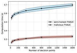
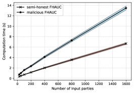
Figure 2: The AUC computation time of FHAUC. Evaluated for both the semi-honest and malicious settings against (a) the number of decision points for a fixed number of 15 parties and (b) the number of parties for a fixed number of decision points ($N=100$).

Dataset: For FHAUC performance analysis, we chose the Criteo dataset, consistent with Sun et al.’s evaluation of DPAUC. Criteo is a large-scale industrial binary classification dataset with approximately 45 million samples, consisting of 26 categorical and 13 real-valued features. We followed the data pre-processing steps outlined by Sun et al. to maintain consistency (Sun et al., 2022). Mirroring Sun et al.’s approach, our training data comprised $90\%$ of the entire Criteo dataset, with the remaining $10\%$ used for test data. We computed AUC on the test set, which included $458,407$ samples, along with various other data sizes randomly sampled from within the remaining $10\%$ of the Criteo dataset.

Model: For our model, we trained a modified DLRM (Deep Learning Recommendation Model) architecture presented in (Naumov et al., 2019) for 3 epochs. It is crucial to emphasize that our primary objective is to showcase the performance of our proposed AUC computation method and how it compares to the state-of-the-art, and thus, the performances of the models are not our primary concern.

Ground-truth AUC: To assess the approximation performance, we compare FHAUC and DPAUC using two AUC computation libraries, namely TensorFlow and scikit-learn, and report their computed results as the ground truth. Consistent with the approach of Sun et al., in our experiments, we set $num\_thresholds=1,000$ for TensorFlow and utilized the default values for other parameters.

Comparison Metric: For DPAUC, following Sun et al., we run the same setting for 100 times and report the corresponding mean and standard deviation of the computed AUC as our comparison metric.

5.1 Performance Analysis

We compare the approximation performance of FHAUC and DPAUC against the ground truth AUC score computed using the libraries described above. To implement DPAUC, we utilized diffprivlib (Holohan et al., 2019), a general-purpose differential privacy library for Python developed by IBM. In all our experiments, we set $\epsilon$ to $1$ and $8$ for DPAUC, representing the smallest and largest privacy budgets used by (Sun et al., 2022) to evaluate the effectiveness of their method while providing the most and least privacy, respectively. We employed 15 participants in the FL system, and each data sample was uniformly distributed at random among the participants. As FHAUC operates deterministically, the number of participants in the FL system and the data distribution among them do not influence the resulting AUC of our method. The only factors influencing the resulting AUC of FHAUC are the number of decision points used by the participants and the total number of global data samples.

Table 1 presents the performance of FHAUC and DPAUC against the ground truth with varying numbers of decision points and different amounts of global data. Because the approximation performance of our method in both the semi-honest and the malicious setting is the same, we did not report it twice for convenience. Observing Table 1, we can see that FHAUC not only provides complete data privacy against both semi-honest and malicious adversaries but also consistently outperforms DPAUC in terms of approximation performance. Moreover, increasing the number of decision points leads to improved approximation performance for FHAUC, but it reduces the performance of DPAUC. This is because in DPAUC, the noise introduced by the input parties scales with the number of decision points utilized by the input parties. Since the amount of noise being added in DPAUC is independent of the data size, this leads to completely unusable approximations when the global data size is small, as clearly shown in Table 1. In contrast, the AUC scores computed by FHAUC are robust and independent of the global data size. Moreover, as FHAUC is deterministic, it consistently produces the same result in every run. This consistency remains unchanged even when the data is distributed in a Non-IID setting among the input parties.

5.2 Computation Time

Finally, we examined the computation time required for the aggregator to compute the AUC of an FL system using malicious FHAUC and semi-honest FHAUC. The computation times are analyzed based on the number of participants and the number of decision points used, as depicted in Figure 2. To assess the impact of the number of decision points on the computation time, we maintain a constant number of 15 participants within the FL system. Similarly, the influence of the number of parties on the computation time is evaluated while keeping the number of decision points $N=100$ constant. As for the malicious FHAUC, we set $S=4$.

Because FHAUC utilizes SIMD (Single Instruction Multiple Data) support provided by OpenFHE (Al Badawi et al., 2022), the AUC computation is highly efficient despite employing FHE. As an example, our method is capable of computing the AUC of an FL system with 100 parties with $99.93\%$ accuracy in just $0.68$ seconds, regardless of data size. As depicted in Figure 2, we observe a logarithmic relationship between the number of decision points used and the computation time of FHAUC. Upon examining Figure 2, we observe a linear relationship between the number of parties and the computation time. Comparing semi-honest FHAUC against malicious FHAUC, we see that the computation time of the malicious setting is almost double for all settings. This is to be expected because the AUC computation is performed twice in the malicious setting.

Although the computation times of our method are well within the range for real-time use, it is important to note that all the results presented here were obtained using a single core. In a real-life FL setting, the aggregator is typically an entity with significantly more computational power, often utilizing multiple cores. Since the aggregation process in FHAUC is suitable for parallelization, the computation time is expected to be significantly faster than what is depicted in Figure 2 when performed by the aggregator in a real-life scenario.

6 Conclusion

In this paper, our focus was on preserving privacy during the model evaluation phase in Horizontal FL systems. We show that the state-of-the-art DP-based AUC computation method in FL systems becomes completely impractical and yields unusable AUC computations when the global test data size is small. Moreover, It also requires a trusted central entity, providing no security against malicious central entities. To address these challenges, we propose a novel AUC computation method that leverages FHE. Our method enables the computation of AUC values for global Horizontal FL models while providing zero information leakage in settings involving both a semi-honest aggregator and input parties, as well as a malicious aggregator.

Through our security analysis, we demonstrate that our method protects AUC computation against malicious adversaries, and any attempts to tamper with the data can easily be detected by the input parties. Furthermore, through empirical results, we have shown that our proposed method provides highly accurate and robust AUC approximations, surpassing the performance of the state-of-the-art DP-based AUC computation method. Finally, we have showcased the scalability of our method in terms of computation time across various settings and demonstrated its practical applicability in real-life FL systems.

Our proposed method not only guarantees complete privacy but also ensures computation robustness and provides security against a malicious aggregator. To the best of our knowledge, FHAUC is the first method to utilize FHE for privacy-preserving model evaluation in FL systems while providing security against both semi-honest and malicious aggregators.

Appendix A ROC Curve and AUC

The ROC curve plots False Positive Rate (FPR) on the x-axis and True Positive Rate (TPR) on the y-axis. TPR for a given threshold value $\theta$ is defined as $\textit{TPR}^{\theta}=\frac{TP^{\theta}}{TP^{\theta}+FN^{\theta}}$, where True Positive is denoted as $TP$ and False Negative as $FN$. Similarly, FPR for a given threshold value $\theta$ is defined as $\textit{FPR}^{\theta}=\frac{FP^{\theta}}{FP^{\theta}+TN^{\theta}}$, where False Positive is denoted as $FP$ and True Negative as $TN$.

The AUC is obtained by measuring the area between the ROC curve and the x-axis. Calculating the AUC depends on the specific problem and available information. For a binary classification problem with $\mathcal{D}$ test samples, the AUC of the ROC curve can be computed as follows:

$$AUC=\sum_{i=1}^{\mathcal{D}}\frac{(TPR^{i}+TPR^{i-1})\cdot(FPR^{i}-FPR^{i-1})}{2}$$ (3)

If we observe Equation 3, we can see that the formula makes use of the TPR and FPR values to compute the AUC. However, using either of these equations poses a challenge if we would like to compute the AUC through FHE since it is difficult to perform division in FHE schemes. In order to minimize the number of division operations, Equation 3 can be rewritten by replacing $TPR^{i}$ with $\frac{TP^{i}+TP^{i-1}}{TP^{\mathcal{D}}}$ and $FPR^{i}$ with $\frac{FP^{i}-FP^{i-1}}{FP^{\mathcal{D}}}$ as follows:

$$\begin{split}AUC&=\sum_{i=1}^{\mathcal{D}}\frac{(TPR^{i}+TPR^{i-1})\cdot(FPR^{i}-FPR^{i-1})}{2}\\ &=\sum_{i=1}^{\mathcal{D}}\frac{(\frac{TP^{i}}{TP^{\mathcal{D}}}+\frac{TP^{i-1}}{TP^{\mathcal{D}}})\cdot(\frac{FP^{i}}{FP^{\mathcal{D}}}-\frac{FP^{i-1}}{FP^{\mathcal{D}}})}{2}\\ &=\sum_{i=1}^{\mathcal{D}}\frac{(\frac{TP^{i}+TP^{i-1}}{TP^{\mathcal{D}}})\cdot(\frac{FP^{i}-FP^{i-1}}{FP^{\mathcal{D}}})}{2}\\ &=\sum_{i=1}^{\mathcal{D}}\frac{(TP^{i}+TP^{i-1})\cdot(FP^{i}-FP^{i-1})}{2\cdot TP^{\mathcal{D}}\cdot FP^{\mathcal{D}}}\\ &=\frac{\sum_{i=1}^{\mathcal{D}}(TP^{i}+TP^{i-1})\cdot(FP^{i}-FP^{i-1})}{2\cdot TP^{\mathcal{D}}\cdot FP^{\mathcal{D}}}\end{split}$$ (4)

Notice that only a single division operation is enough to compute the AUC. We make use of this property to compute the AUC while utilizing FHE.

Appendix B DPAUC and its Limitations

In this section, we provide a detailed discussion of the current state-of-the-art solution, namely DPAUC (Sun et al., 2022), and then discuss its limitations through empirical results.

B.1 Method

The high-level method of DPAUC is similar to the semi-honest setting of our method. In DPAUC, upon receiving the global model, participants in the FL system compute their TP, FP, TN, and FN statistics based on a set of decision points $S_{N}$ with a fixed size. Then, each client adds Laplacian noise with a total privacy budget of $\epsilon\in\{1,2,4,8\}$ to their statistics. The amount of noise added depends on the number of decision points that are utilized. These noisy statistics are then transmitted to the aggregator to compute the global AUC.

While differential privacy is achieved through noise addition, there are several limitations with this approach in terms of both privacy and approximation performance.

B.2 Information Leakage in DPAUC

Although differential privacy is achieved, due to the complementary nature of TP, FN, FP, and TN statistics, aggregating TP with FN and FP with TN reveals the noisy count of positive and negative samples within the local test data, respectively. By averaging these noisy statistics, a semi-honest aggregator can infer the approximate number of total, as well as positively and negatively labeled samples owned by each input party.

Table 2: Prediction Error of the Semi-Honest Aggregator in terms of samples for DPAUC

				Prediction Err. (in samples)
$\epsilon$	$N$	$\epsilon^{\prime}$	Total Samples	Positive samples	Negative samples
	$25$	$0.01$	$7.33\pm 61.43$	$3.31\pm 38.93$	$2.99\pm 39.25$
$1$	$50$	$0.005$	$11.97\pm 81.51$	$3.21\pm 55.20$	$3.55\pm 54.86$
	$100$	$0.0025$	$8.97\pm 109.73$	$3.56\pm 80.42$	$3.72\pm 81.03$
	$25$	$0.02$	$0.52\pm 30.14$	$1.76\pm 19.81$	$1.66\pm 20.11$
$2$	$50$	$0.01$	$2.69\pm 39.89$	$1.04\pm 28.08$	$1.34\pm 28.73$
	$100$	$0.005$	$3.02\pm 55.02$	$1.47\pm 40.13$	$1.90\pm 40.74$
	$25$	$0.04$	$0.33\pm 14.70$	$0.29\pm 9.90$	$0.33\pm 10.10$
$4$	$50$	$0.02$	$1.21\pm 19.89$	$0.66\pm 13.72$	$0.59\pm 12.88$
	$100$	$0.01$	$0.26\pm 27.38$	$0.98\pm 20.34$	$1.07\pm 21.13$
	$25$	$0.08$	$0.13\pm 7.41$	$0.02\pm 4.49$	$0.01\pm 5.55$
$8$	$50$	$0.04$	$0.88\pm 9.76$	$0.02\pm 6.77$	$0.02\pm 7.09$
	$100$	$0.02$	$0.16\pm 13.72$	$0.15\pm 10.11$	$0.11\pm 9.91$

Table 2 displays the average prediction error of the semi-honest aggregator (average and standard deviation of 100 runs), in terms of total, positively, and negatively labeled samples, based on different $\epsilon$ and $N$ for a single input party when utilizing DPAUC. It is important to mention that these results are independent of the number of samples the input parties have, meaning the accuracy of the attack depends only on $\epsilon$ and $N$. This is particularly significant because it implies that if the number of samples owned by an input party is large, the aggregator can confidently approximate the exact number. To illustrate, if an input party has a total of $100000$ samples in their test data, even with a total privacy budget of $\epsilon=1$ and $N=100$, which represents the smallest privacy budget used by (Sun et al., 2022) to test the performance of DPAUC while ensuring maximum privacy, the aggregator can infer the approximate number of samples with an error of only $0.0011\%$ on average. Moreover, the aggregator can also infer the total number of positively and negatively labeled samples owned by an input party, as shown in Table 2. Additionally, DPAUC enables accurate AUC approximations on large datasets, allowing the semi-honest aggregator to infer local AUC scores and the global AUC score. In contrast, our FHE-based method ensures complete data privacy against both semi-honest aggregators and input parties.

Another limitation of DPAUC is its vulnerability to a malicious aggregator. Privacy analysis of DPAUC (Sun et al., 2022) assumes a trusted central entity, which may not align with real-world FL systems. As computations are performed on plaintext, a malicious aggregator can manipulate statistics, including discarding party data and reporting random AUC scores. Furthermore, verification by input parties regarding the integrity of the obtained AUC score at the end of the protocol is impossible. In contrast, our method, operating in a malicious setting, detects and verifies any tampering attempts by the aggregator, providing security against malicious behavior, as proven in our security analysis.

B.3 Performance of DPAUC

In DPAUC, the noise introduced by the input parties scales with the number of decision points, where $\epsilon=N*(\epsilon_{TP}+\epsilon_{FP}+\epsilon_{TN}+\epsilon_{FN})$. Sun et al. (Sun et al., 2022) report that they set $\epsilon_{TP}=\epsilon_{FP}=\epsilon_{TN}=\epsilon_{FN}=\epsilon^{\prime}$, resulting in a total privacy budget of $4N\epsilon^{\prime}$. Because the amount of noise being added is independent of the data size, this leads to completely unusable AUC approximations when the global data size is small. The performance of DPAUC across different global data sizes is not addressed at all by Sun et al., although it significantly influences the performance of their method. They utilize a single dataset comprising 458,407 global samples in total to demonstrate the effectiveness of DPAUC. Consequently, their approximation performance is shown to be satisfactory.

To highlight the weakness of DPAUC with limited global data sizes, we compared DPAUC and our method across two datasets with varying global test samples. The first dataset we used to showcase the performance of FHAUC against DPAUC was the Criteo dataset, which is the same dataset used in (Sun et al., 2022) (Section 5). To compare the performance of both methods further, we additionally used an image classification dataset. The dataset comprises over 200,000 images of celebrities for gender prediction tasks. Each image is of size $178\times 218$ pixels and is in color. We chose an image classification dataset to maximize the number of threshold samples, thereby allowing for a clearer observation of the performance of both FHAUC and DPAUC. As for the model, we employed a basic CNN architecture comprising 13 layers and trained the model for 4 epochs. The performance of both FHAUC and DPAUC on the gender classification dataset is shown in Table 3.

Data Size	TensorFlow	scikit-learn	$N$	FHAUC	DPAUC ($\epsilon=1$)	DPAUC ($\epsilon=8$)
			$25$	$0.893400\pm 0.0$	$63.00177\pm 723.6120$	$-0.97248\pm 28.83271$
$10^{2}$	$0.891400$	$0.891600$	$50$	$0.888800\pm 0.0$	$87.28492\pm 787.6992$	$-43.2448\pm 496.1687$
			$100$	$0.892600\pm 0.0$	$244.4928\pm 2981.016$	$-93.4737\pm 657.0762$
			$25$	$0.937070\pm 0.0$	$8.817562\pm 408.6866$	$0.991520\pm 0.320545$
$10^{3}$	$0.938614$	$0.938588$	$50$	$0.938250\pm 0.0$	$127.9842\pm 1369.205$	$2.261357\pm 9.195085$
			$100$	$0.938700\pm 0.0$	$253.1984\pm 2616.424$	$8.875182\pm 50.45507$
			$25$	$0.909860\pm 0.0$	$1.009118\pm 0.249137$	$0.904852\pm 0.027761$
$10^{4}$	$0.911410$	$0.911406$	$50$	$0.910900\pm 0.0$	$1.387757\pm 1.807835$	$0.914889\pm 0.057772$
			$100$	$0.911290\pm 0.0$	$10.76247\pm 102.0806$	$0.894566\pm 0.115002$
			$25$	$0.950080\pm 0.0$	$0.947500\pm 0.022812$	$0.950197\pm 0.003212$
$10^{5}$	$0.954020$	$0.954052$	$50$	$0.952370\pm 0.0$	$0.950787\pm 0.049092$	$0.953180\pm 0.006660$
			$100$	$0.953422\pm 0.0$	$0.980881\pm 0.103526$	$0.953366\pm 0.011731$

Table 3: Performance analysis of FHAUC compared to DPAUC on gender classification dataset with $\epsilon=1,8$ and with 15 parties.

Observing Table 3, we can see that the results consistently show FHAUC outperforming DPAUC regardless of dataset complexity, as the deterministic nature of FHAUC ensures reliable AUC computations independent of data size.

Appendix C Security Analysis

C.1 Security Analysis of Semi-honest FHAUC

For correctness, we need to prove that the semi-honest aggregator can compute the AUC value as defined in Equation 2. In semi-honest FHAUC, each client $m\in\{1,\dots,(M-1)\}$ sends

$$E_{K}(TP^{n}_{m}+TP^{n-1}_{m}),$$

$$E_{K}(TP^{n}_{m}+TP^{n-1}_{m}),$$

$$E_{K}(TP^{N-1}_{m}),E_{K}(FP^{N-1}_{m})$$

to the aggregator for each $n\in\{1,\dots,(N-1)\}$. The semi-honest aggregator adds corresponding homomorphically encrypted values of all input parties using homomorphic operations. Subsequently, it can compute the encrypted numerator and denominator of Equation 2 with homomorphic operations on the aggregated encrypted values.

We examine the information that can be obtained by a semi-honest aggregator and input parties. The analysis is based on the following assumptions:

1. The aggregator cannot decrypt the shared ciphertexts without access to the private key.

2. The communication between the participants and the aggregator is secure.

3. The distribution of the FHE private key is performed through a secure channel.

The local prediction confidence values and their distributions, label information, and number of samples for each client are never shared and, therefore, cannot be known by a semi-honest aggregator due to the nature of the algorithm. The values $\text{T}^{n}$ and $\text{F}^{n}$ for $n\in\{n,\ldots,(N-1)\}$ are the only information that each participant shares with the aggregator. Since all of these values are encrypted, the sm-honest aggregator can not obtain the plain $T^{n}$ and $F^{n}$ values based on Assumption 1. Similarly, the num and denom computed by the aggregator at the end of the algorithm are also encrypted, which makes it similarly impossible for the aggregator to obtain the performance of the global model based on Assumption 1. Therefore, the only information that the semi-honest aggregator can infer is the number of decision points used by the participants to compute the AUC by observing the size of the ciphertexts. Since this information is not inherent to the participants’ local data, the semi-honest FHAUC ensures zero information leakage against a semi-honest aggregator.

In FHAUC, we aim to preserve the sensitive information of an input party from not only the aggregator but also the other input parties. The only possibility of occurrence of such leakage is via the outsourced division operation by the aggregator. Due to the lack of division operation in OpenFHE, the aggregator has to send the numerator and the denominator of AUC to the input parties. However, allowing the input parties to obtain these values without any masking has a possible privacy leakage. As an illustrative example of this leakage, in the edge case where we have two input parties and the denominator is the multiplication of two prime numbers, the input parties can identify the number of samples of the other input party as well as its class distribution. Since the denominator of AUC is the multiplication of the total number of samples labeled as positive and negative, a denominator that is the multiplication of two prime numbers has only one pair of values satisfying its value. If the number of positive samples or the number of negative samples of the input party is larger than any of the multipliers of the denominator, then the input party can exactly deduce which multiplier is the total number of samples labeled as positive and which one is the total number of samples labeled as negative. Once this information is obtained, the input party can deduce the total number of samples of the other input party and its class distribution.

Such an exact inference has a low chance of occurrence, but we wanted to reduce it to an even more negligible probability by sending $E_{K}(num\cdot d+denom\cdot c)$, $E_{K}(denom\cdot d)$, and $\frac{c}{d}$ instead of $E_{K}(num)$ and $E_{K}(denom)$ where $c$ and $d$ are floating-point values and even further increase the search space of the integer multipliers of the denominator. Assume that we have candidate $c^{\prime}$ and $d^{\prime}$ satisfying that $\frac{c^{\prime}}{d^{\prime}}=\frac{c}{d}$ and $num^{\prime}=\frac{num\cdot c}{c^{\prime}}=\frac{num\cdot d}{d^{\prime}}$ and $denom^{\prime}=\frac{denom\cdot c}{c^{\prime}}=\frac{denom\cdot d}{d^{\prime}}$ are integers. Besides $denom^{\prime}$, we can come up with another candidate by computing $c^{\prime\prime}=\frac{c^{\prime}}{I}$ and $d^{\prime\prime}=\frac{d^{\prime}}{I}$ where $I\geq 2$ is an integer and this results in $denom^{\prime\prime}=denom^{\prime}\cdot I$. On top of the factors of $denom^{\prime}$, the factors of $I$ will be added and it increases the possible pairs of multipliers of $denom$, reducing the chance of estimating the correct pair of multipliers of $denom$ to a negligible probability.

C.2 Security Analysis of Malicious FHAUC

In this section, we analyze the security of the malicious FHAUC scheme and demonstrate its satisfaction with properties like correctness, completeness, soundness, and security.

Correctness: A scheme is correct if any honest computation will decrypt to the expected result (Viand et al., 2023).

We demonstrate that conducting the homomorphic computation on the encrypted randomized values, following the protocol description, consistently yields the expected results: $E_{K}(r_{0}\cdot\text{num}+r_{1}\cdot\text{denom})$ and $E_{K}(r_{2}\cdot\text{denom})$. The details of correctness analysis is given in Section C.2 of the Appendix.

Soundness: A scheme is sound if the adversary cannot make the verification accept an incorrect answer (Viand et al., 2023).

The adversary needs to modify inputs, intermediate values, output, or the secure protocol execution in a way that the outputs of two computations yield the same modified AUC value.

$$\frac{r_{2}}{r_{0}}(\frac{r_{0}\cdot\text{num}+r_{1}\cdot\text{denom}}{r_{2}\cdot\text{denom}}-\frac{r_{1}}{r_{2}}) =\frac{r_{2}^{\prime}}{r_{0}^{\prime}}(\frac{r_{0}^{\prime}\cdot\text{num}+r_{1}^{\prime}\cdot\text{denom}}{r_{2}^{\prime}\cdot\text{denom}}-\frac{r_{1}^{\prime}}{r_{2}^{\prime}})$$

The adversary cannot discard or modify the contributions $\text{T}^{n}_{m}[s]$ and $\text{F}^{n}_{m}[s]$ of a specific input party $m$ to $\text{T}^{n}[s]$ and $\text{F}^{n}[s]$. This impossibility arises because $\text{T}^{n}_{m}[s]$ and $\text{F}^{n}_{m}[s]$ are randomized using zero-sum random numbers shared among all input parties. Attempting to discard or modify these contributions from the input party does not eliminate the zero-sum random values. Furthermore, the adversary is unable to alter the contributions of an input party to a specific $\text{T}^{n}_{m}[s]$ or $\text{F}^{n}_{m}[s]$ since these contributions are ordered differently in two secure computations, each relying on a distinct random permutation unknown to the adversary. The probability of the adversary guessing the locations of these specific contributions is $(\frac{S!(SN-S)!}{SN!})^{2}$.

The adversary may attempt to discard or alter the aggregated contributions $\text{T}^{n}[s]$ and $\text{F}^{n}[s]$. Initially, the adversary may target the $\text{T}^{n}[s]$ and $\text{F}^{n}[s]$ values associated with a specific decision boundary. However, this action is not computationally feasible due to the differing order of aggregated contributions in two secure computations. The adversary’s ability to accurately identify the order of a particular contribution in both secure computations stands at a probability of $(\frac{S!(SN-S)!}{SN!})^{2}$. Secondly, the adversary may attempt to discard or modify the $\text{T}^{n}[s]$ and $\text{F}^{n}[s]$ values associated with all decision boundaries. To achieve this, the adversary seeks to locate $\text{T}^{N-1}[s]$ and $\text{F}^{N-1}[s]$, which aren’t linked to any specific decision boundaries and are randomized using scalar values $r_{5}$ and $r_{6}$, while those associated with decision boundaries use scalar values $r_{3}$ and $r_{4}$. However, this attempt is also computationally infeasible due to the different order of aggregated contributions in the two secure computations. The adversary’s ability to accurately determine the order of $\text{T}^{N-1}[s]$ and $\text{F}^{N}-1[s]$ in both secure computations is constrained by a probability of $(\frac{S!(SN-S)!}{SN!})^{2}$.

The adversary might try to alter $E_{K}(r_{0}\cdot\text{num}+r_{1}\cdot\text{denom})$, $E_{K}(r_{2}\cdot\text{denom})$, $E_{K}(r_{0}^{\prime}\cdot\text{num}+r_{1}^{\prime}\cdot\text{denom})$, and $E_{K}(r_{2}^{\prime}\cdot\text{denom})$ to make two computations produce the same modified AUC. The adversary’s attempt to guess these 32-bit random numbers remains impossible as all values within the computation are homomorphically encrypted, making it impossible for the adversary to verify her guesses. Moreover, the computational infeasibility of this verification is compounded by the probability of correctly guessing only three 32-bit random numbers in a single secure computation, which stands at $\frac{1}{2^{96}}$ a statistically negligible probability and computationally impractical to achieve.

The split count $S$ is a critical parameter defining the security level of the malicious FHAUC scheme. The choice of $S$ significantly impacts the success probability of the malicious aggregator to modify inputs, intermediate values, output, or the secure protocol execution in a way that the outputs of two computations yield the same modified AUC value. There is an inverse relationship between the number of decision points $N$ and $S$. Increasing $S$ while decreasing $N$ effectively reduces the success probability of the malicious aggregator. For instance, with $N=100$ and $S=7$, the success probability is $\frac{1}{2^{107}}$. With $N=100$ and $S=4$, the success probability reduces to $\frac{1}{2^{60}}$. Similarly, for $N=25$ and $S=9$, the success probability becomes $\frac{1}{2^{103}}$.

In our security analysis, we make the assumption that the malicious aggregator has knowledge of $S$. However, in a real-life scenario, the aggregator does not know $S$ and must attempt to guess this value at the beginning of any attack. Our analysis does not factor in the success probability of the malicious aggregator correctly guessing $S$. Instead, we assume that $S$ is already known to the malicious adversary. Nonetheless, if we consider the success probability of the malicious aggregator in guessing $S$, the likelihood of successfully modifying the AUC decreases drastically. Moreover, in malicious FHAUC, the input parties use the same $S$ value for each $T^{n}$ and $F^{n}$. Yet, it is possible to choose different $S$ values for each $T^{n}$ and $F^{n}$. This significantly reduces the success probability for the malicious adversary, making it nearly impossible to modify the AUC.

Security: Our verification method in the malicious FHAUC primarily relies on homomorphic decryption. To compromise the security of the verification method in malicious FHAUC, the adversary would need to break the security of the underlying FHE scheme, CKKS, the security of which has been formally proven in (Cheon et al., 2017).

References

- Al Badawi et al. (2022) Al Badawi, A., Bates, J., Bergamaschi, F., Cousins, D. B., Erabelli, S., Genise, N., Halevi, S., Hunt, H., Kim, A., Lee, Y., et al. Openfhe: Open-source fully homomorphic encryption library. In Proceedings of the 10th Workshop on Encrypted Computing & Applied Homomorphic Cryptography, pp. 53–63, 2022.
- Aono et al. (2017) Aono, Y., Hayashi, T., Wang, L., Moriai, S., et al. Privacy-preserving deep learning via additively homomorphic encryption. IEEE transactions on information forensics and security, 13(5):1333–1345, 2017.
- Bonawitz et al. (2019) Bonawitz, K., Eichner, H., Grieskamp, W., Huba, D., Ingerman, A., Ivanov, V., Kiddon, C., Konečný, J., Mazzocchi, S., McMahan, B., Van Overveldt, T., Petrou, D., Ramage, D., and Roselander, J. Towards federated learning at scale: System design. In Talwalkar, A., Smith, V., and Zaharia, M. (eds.), Proceedings of Machine Learning and Systems, volume 1, pp. 374–388, 2019.
- Cheon et al. (2017) Cheon, J. H., Kim, A., Kim, M., and Song, Y. Homomorphic encryption for arithmetic of approximate numbers. In Advances in Cryptology–ASIACRYPT 2017: 23rd International Conference on the Theory and Applications of Cryptology and Information Security, Hong Kong, China, December 3-7, 2017, Proceedings, Part I 23, pp. 409–437. Springer, 2017.
- ElGamal (1985) ElGamal, T. A public key cryptosystem and a signature scheme based on discrete logarithms. IEEE transactions on information theory, 31(4):469–472, 1985.
- Fang & Qian (2021) Fang, H. and Qian, Q. Privacy preserving machine learning with homomorphic encryption and federated learning. Future Internet, 13(4):94, 2021.
- Foster et al. (2014) Foster, K. R., Koprowski, R., and Skufca, J. D. Machine learning, medical diagnosis, and biomedical engineering research-commentary. Biomedical engineering online, 13:1–9, 2014.
- Gentry (2009) Gentry, C. Fully homomorphic encryption using ideal lattices. In Proceedings of the forty-first annual ACM symposium on Theory of computing, pp. 169–178, 2009.
- Holohan et al. (2019) Holohan, N., Braghin, S., Mac Aonghusa, P., and Levacher, K. Diffprivlib: the IBM differential privacy library. ArXiv e-prints, 1907.02444 [cs.CR], July 2019.
- Kairouz et al. (2021) Kairouz, P., McMahan, H. B., Avent, B., Bellet, A., Bennis, M., Bhagoji, A. N., Bonawitz, K., Charles, Z., Cormode, G., Cummings, R., et al. Advances and open problems in federated learning. Foundations and Trends® in Machine Learning, 14(1–2):1–210, 2021.
- Kononenko (2001) Kononenko, I. Machine learning for medical diagnosis: history, state of the art and perspective. Artificial Intelligence in medicine, 23(1):89–109, 2001.
- Li et al. (2020) Li, T., Sahu, A. K., Talwalkar, A., and Smith, V. Federated learning: Challenges, methods, and future directions. IEEE signal processing magazine, 37(3):50–60, 2020.
- Liu et al. (2019) Liu, C., Chakraborty, S., and Verma, D. Secure model fusion for distributed learning using partial homomorphic encryption. Policy-Based Autonomic Data Governance, pp. 154–179, 2019.
- Matthews & Harel (2013) Matthews, G. J. and Harel, O. An examination of data confidentiality and disclosure issues related to publication of empirical roc curves. Academic radiology, 20(7):889–896, 2013.
- McMahan & Ramage (2017) McMahan, B. and Ramage, D. Federated learning: Collaborative machine learning without centralized training data. Google AI Blog, 04 2017.
- McMahan et al. (2017) McMahan, B., Moore, E., Ramage, D., Hampson, S., and y Arcas, B. A. Communication-efficient learning of deep networks from decentralized data. In Artificial intelligence and statistics, pp. 1273–1282. PMLR, 2017.
- Mothukuri et al. (2021) Mothukuri, V., Parizi, R. M., Pouriyeh, S., Huang, Y., Dehghantanha, A., and Srivastava, G. A survey on security and privacy of federated learning. Future Generation Computer Systems, 115:619–640, 2021. ISSN 0167-739X. doi: https://doi.org/10.1016/j.future.2020.10.007.
- Naumov et al. (2019) Naumov, M., Mudigere, D., Shi, H.-J. M., Huang, J., Sundaraman, N., Park, J., Wang, X., Gupta, U., Wu, C.-J., Azzolini, A. G., et al. Deep learning recommendation model for personalization and recommendation systems. arXiv preprint arXiv:1906.00091, 2019.
- Paillier (1999) Paillier, P. Public-key cryptosystems based on composite degree residuosity classes. In International conference on the theory and applications of cryptographic techniques, pp. 223–238. Springer, 1999.
- Rivest et al. (1978) Rivest, R. L., Shamir, A., and Adleman, L. A method for obtaining digital signatures and public-key cryptosystems. Communications of the ACM, 21(2):120–126, 1978.
- Sav et al. (2022) Sav, S., Bossuat, J.-P., Troncoso-Pastoriza, J. R., Claassen, M., and Hubaux, J.-P. Privacy-preserving federated neural network learning for disease-associated cell classification. Patterns, 3(5), 2022.
- Stoddard et al. (2014) Stoddard, B., Chen, Y., and Machanavajjhala, A. Differentially private algorithms for empirical machine learning. arXiv preprint arXiv:1411.5428, 2014.
- Sun et al. (2022) Sun, J., Yang, X., Yao, Y., Xie, J., Wu, D., and Wang, C. Dpauc: Differentially private auc computation in federated learning. arXiv preprint arXiv:2208.12294, 2022.
- Ünal et al. (2023) Ünal, A. B., Pfeifer, N., and Akgün, M. ppaurora: Privacy preserving area under receiver operating characteristic and precision-recall curves. In Li, S., Manulis, M., and Miyaji, A. (eds.), Network and System Security, pp. 265–280, Cham, 2023. Springer Nature Switzerland. ISBN 978-3-031-39828-5.
- Viand et al. (2023) Viand, A., Knabenhans, C., and Hithnawi, A. Verifiable fully homomorphic encryption. arXiv preprint arXiv:2301.07041, 2023.
- Wei et al. (2020) Wei, K., Li, J., Ding, M., Ma, C., Yang, H. H., Farokhi, F., Jin, S., Quek, T. Q., and Poor, H. V. Federated learning with differential privacy: Algorithms and performance analysis. IEEE Transactions on Information Forensics and Security, 15:3454–3469, 2020.
- Yeh et al. (2002) Yeh, S.-T. et al. Using trapezoidal rule for the area under a curve calculation. Proceedings of the 27th Annual SAS® User Group International (SUGI’02), pp. 1–5, 2002.
- Zhang et al. (2020) Zhang, C., Li, S., Xia, J., Wang, W., Yan, F., and Liu, Y. Batchcrypt: Efficient homomorphic encryption for cross-silo federated learning. In Proceedings of the 2020 USENIX Annual Technical Conference (USENIX ATC 2020), 2020.
- Zhao et al. (2020) Zhao, B., Mopuri, K. R., and Bilen, H. idlg: Improved deep leakage from gradients. arXiv preprint arXiv:2001.02610, 2020.
- Zhu et al. (2019) Zhu, L., Liu, Z., and Han, S. Deep leakage from gradients. Advances in neural information processing systems, 32, 2019.