Task-optimal data-driven surrogate models for eNMPC via differentiable simulation and optimization

Abstract

We present a method for end-to-end learning of Koopman surrogate models for optimal performance in control. In contrast to previous contributions that employ standard reinforcement learning (RL) algorithms, we use a training algorithm that exploits the potential differentiability of environments based on mechanistic simulation models. We evaluate the performance of our method by comparing it to that of other controller type and training algorithm combinations on a literature known eNMPC case study. Our method exhibits superior performance on this problem, thereby constituting a promising avenue towards more capable controllers that employ dynamic surrogate models.

I INTRODUCTION

Data-driven surrogate models for computationally expensive mechanistic dynamic models can enable real-time economic nonlinear model predictive control (eNMPC) by reducing the computational burden of solving the underlying optimal control problems [1]. Recent articles [2, 3, 4] have established end-to-end reinforcement learning (RL) of dynamic surrogate models as an alternative to the prevalent system identification (SI) approach. These approaches yield increased performance of the resulting controllers regarding the respective control objective, e.g., the minimization of operating costs while avoiding constraint violations. RL algorithms are a class of policy optimization algorithms that enable learning of optimal controllers through trial-and-error actuation of real-world environments [5]. Standard RL algorithms view environments as black boxes and do not use derivative information regarding the environment dynamics or the reward signals, even though many RL publications use simulated environments where analytical gradients of dynamics and rewards could be available. Recently, policy optimization algorithms that leverage derivative information from simulated environments were designed [6, 7] and have shown enhanced training wall-clock time efficiency and increased terminal performance compared to state-of-the-art RL algorithms. These algorithmic advances could also benefit the learning of dynamic surrogate models for (eN)MPC if a differentiable mechanistic simulation model is available. Nevertheless, policy optimization using differentiable environments has yet to be established for the learning of dynamic surrogate models for (eN)MPC.

Policy gradient algorithms are the most commonly used class of RL algorithms for end-to-end learning of dynamic models for control, see, e.g., [2, 3]. However, fundamental issues arise from the fact that policy gradient algorithms do not leverage analytical gradients from the environment. These issues concern both our understanding of the algorithms’ empirical behavior [8, 9], and their performance [10, 11, 12]. To overcome the problems associated with policy gradient algorithms, differentiable simulators, e.g., [13], can be used to construct simulated RL environments with automatically differentiable dynamics and reward functions, thus enabling the use of analytic gradients for policy optimization. Recent algorithmic advances [6, 7] manage to avoid the well-known problems of Backpropagation Through Time (BPTT) [14], i.e., noisy optimization landscapes and exploding/vanishing gradients [15, 7].

Task-optimal dynamic models for control can be learned by viewing a dynamic model and its learnable parameters as part of a differentiable policy. This policy consists of the dynamic model and a differentiable optimal control algorithm. Various methods for turning (e)NMPC controllers into differentiable and thereby learnable policies have been developed, see, e.g., [16, 3, 4]. These methods do not depend on any specific policy optimization algorithm. Therefore, the advantages in terminal performance using policy optimization algorithms that capitalize on derivative information from the environment [6, 7] could be transferable from the task of learning generic neural network controllers to the learning of task-optimal dynamic models for (e)NMPC.

By combining our previously proposed method for end-to-end learning of task-optimal Koopman models in (e)NMPC applications [4] with the Short-Horizon Actor-Critic (SHAC) algorithm [7], we present a method for end-to-end optimization of Koopman surrogate models. Crucially, our method exploits the differentiability of simulated environments, distinguishing it from previous contributions, which are based on RL [2, 3, 4] or imitation learning [16]. We evaluate the resulting control performance on an (e)NMPC case study derived from a literature-known continuous stirred-tank reactor model [17]. We compare the performance to that of the following policy and training paradigm configurations: MPCs employing Koopman surrogate models that were trained either using (i) system identification or (ii) RL, and model-free neural network policies trained either using (iii) RL or (iv) SHAC. We find that the novel combination of a Koopman-eNMPC trained using SHAC exhibits superior performance compared to the other options. This finding confirms our expectation that the advantages of policy optimization algorithms that leverage derivative information from differentiable environments can apply to the end-to-end training of dynamic models for predictive control applications.

We structure the remainder of this paper as follows: Section II presents our method. Section III showcases the performance of our method on a simulated case study and discusses the results. Section IV draws some final conclusions.

II Method

Subsections II-A - II-C present the preliminaries for our method for learning task-optimal dynamic Koopman surrogate models for control applications, which is subsequently outlined in Subsection II-D.

II-A Policy optimization

We adopt an RL perspective [18] on policy optimization problems. Herein, the control problem is represented by a Markov Decision Process (MDP) with associated states $\bm{x}_{t}\in\mathbb{R}^{n}$ and control inputs $\bm{u}_{t}\in\mathbb{R}^{m}$, a transition function $\bm{\mathcal{F}}\colon\mathbb{R}^{n+m}\to\mathbb{R}^{n}$,

$$\bm{x}_{t+1}=\bm{\mathcal{F}}(\bm{x}_{t},\bm{u}_{t}),$$ (1)

and a scalar reward function $\mathcal{R}\colon\mathbb{R}^{n+m}\mapsto\mathbb{R}$,

$$r_{t+1}=\mathcal{R}(\bm{u}_{t},\bm{x}_{t+1}).$$ (2)

An environment is the MDP of a specific RL problem. An episode refers to a sequence of interactions between a policy and its environment, starting from an initial state, involving a series of control inputs, and leading to a terminal state. The return

$$G_{t}=\sum_{k=0}^{T}\gamma^{k}r_{t+k+1}$$

is the (discounted) sum of rewards over an episode with $T+1$ time steps, starting at time step $t$, with the parameter $\gamma$, $0\leq\gamma\leq 1$, being the discount rate. A policy $\bm{\pi}_{\bm{\theta}}(\bm{u}_{t}|\bm{x}_{t})\colon\mathbb{R}^{n}\mapsto\mathbb{R}^{m}$ is a function, parameterized by $\bm{\theta}$, mapping states $\bm{x}_{t}$ to (probability distributions over) control inputs $\bm{u}_{t}$. The goal of policy optimization is to maximize the expected future return.

II-B Koopman theory for control

Applied Koopman theory aims to find linear representations of nonlinear dynamic systems through a nonlinear transformation of the system states into a higher dimensional Koopman space [19]. Korda and Mezić [20] propose an extension of Koopman theory to controlled systems. The resulting models lead to convex optimal control problems provided that the objective function and any additional constraints do not introduce non-convexity. The models are of the form

$$\bm{z}_{0} =\bm{\psi}_{\bm{\theta}}(\bm{x}_{0}),$$

$$\bm{z}_{t+1} =\bm{A}_{\bm{\theta}}\bm{z}_{t}+\bm{B}_{\bm{\theta}}\bm{u}_{t},$$

$$\hat{\bm{x}}_{t} =\bm{C}_{\bm{\theta}}\bm{z}_{t},$$

where $\bm{z}_{t}\in\mathbb{R}^{N}$ is the vector of Koopman states and $\hat{\bm{x}}_{t}\in\mathbb{R}^{n}$ is the model prediction of the system state at time step $t$. The overall model consists of the following components: A nonlinear encoder $\bm{\psi}_{\bm{\theta}}\colon\mathbb{R}^{n}\mapsto\mathbb{R}^{N}$ that transforms the initial condition $\bm{x}_{0}$ into the Koopman space. $\bm{A}_{\bm{\theta}}\in\mathbb{R}^{N\times N}$ and $\bm{B}_{\bm{\theta}}\in\mathbb{R}^{N\times m}$ linearly advance the Koopman state vector forward in time. $\bm{C}_{\bm{\theta}}\in\mathbb{R}^{n\times N}$ is a linear decoder that transforms a prediction of the Koopman state into a prediction of the system state.

All model components can be trained by adjusting the parameters $\bm{\theta}$. Lusch et al. [21] identify three requirements for autoregressive Koopman models. When performing SI, these requirements result in a training loss function that is a weighted combination of three loss terms. The extension to controlled systems and the model structure by Korda and Mezić [20] results in the following three loss terms:

1. An autoencoder loss term that promotes the identification of nonlinear lifting functions $\bm{\psi_{\theta}}$, which allow for a linear reconstruction of the system state through $\bm{C}_{\bm{\theta}}$:

   $$||\bm{C_{\theta}}\bm{\psi_{\theta}}(\bm{x}_{t})-\bm{x}_{t}||$$ (3)

2. A prediction loss term for the identification of the linear latent space dynamics:

   $$||\bm{A}_{\bm{\theta}}\bm{\psi_{\theta}}(\bm{x}_{t})+\bm{B}_{\bm{\theta}}\bm{u}_{t}-\bm{\psi_{\theta}}(\bm{x}_{t+1})||$$ (4)

3. A loss term combining all elements of the model for the prediction of the original system state:

   $$||\bm{C_{\theta}}(\bm{A}_{\bm{\theta}}\bm{\psi_{\theta}}(\bm{x}_{t})+\bm{B}_{\bm{\theta}}\bm{u}_{t})-\bm{x}_{t+1}||$$ (5)

II-C Short-Horizon Actor-Critic (SHAC) algorithm

SHAC [7] is a policy optimization algorithm that uses derivative information from a differentiable simulation environment, i.e., an environment wherein $\bm{\mathcal{F}}$ and $\mathcal{R}$ (Eq. 1 and 2) are known differentiable functions, to train control policies. Via concatenation using the chain rule, gradients can be propagated through an entire episode [14], thus enabling policy optimization via gradient ascent on returns if the policy is also differentiable. This approach results in the BPTT algorithm for policy optimization, upon which SHAC is based. The concatenation of many backpropagation steps through a differentiable transition function and a differentiable policy, however, leads to exploding/vanishing gradients and to a noisy optimization landscape with many local optima [7], making BPTT unsuitable for long-horizon tasks. SHAC addresses those challenges by shortening the learning horizon, i.e., instead of backpropagating gradients through an entire episode, the episode is split into short-horizon subepisodes for learning. Gradients are not allowed to flow from one subepisode to another. To ensure that the training results in a farsighted policy despite training with short-horizon subepisodes, SHAC uses a value function $V_{\bm{\phi}}$ with learnable parameters $\bm{\phi}$ to estimate future rewards based on the last state of a subepisode. In practice, multiple environment instances can be run in parallel to perform batch updates on the policy and the value function.

II-D Learning task-optimal Koopman models for control

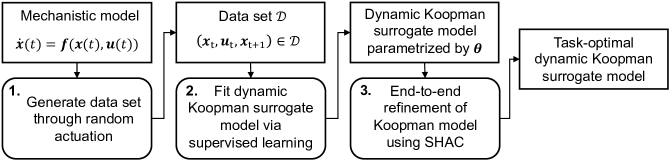
Figure 1: Workflow from mechanistic model to task-optimal dynamic Koopman surrogate model. Adapted from [4].

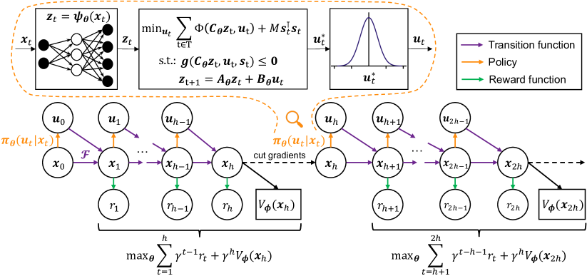
Figure 2: Using SHAC to train a task-optimal Koopman surrogate model: The policy can be optimized by adjusting the parameters $\bm{\theta}$ of the dynamic Koopman surrogate model. $\Phi$ is a convex function for the stage cost of the objective function. To ensure the feasibility of the resulting optimal control problems, we add slack variables $\bm{s}_{t}$ to the state bounds. Their use is penalized quadratically using a penalty factor $M$. Due to the use of PyTorch [22] and cvxpylayers [23], the output $\bm{u}_{t}$ of the policy is differentiable with respect to $\bm{x}_{t}$ and $\bm{\theta}$. The critic is a feedforward neural network with trainable parameters $\bm{\phi}$. To increase the clarity of the figure, we omit the direct dependence of $r_{t+1}$ with respect to $\bm{u}_{t}$.

We aim to exploit the differentiability of continuous-time mechanistic models of the form

$$\dot{\bm{x}}(t)=\bm{f}(\bm{x}(t),\bm{u}(t))$$ (6)

for the end-to-end learning of task-optimal discrete-time dynamic surrogate models. In our previous publication [4], we present a method for end-to-end RL of data-driven Koopman models for optimal performance in (e)NMPC applications, based on viewing the predictive controller as a differentiable policy and training it using RL. This method is independent of the specific policy optimization algorithm. By replacing the RL algorithm [24] with SHAC [7], we can transfer the advantages of policy optimization algorithms that exploit the differentiability of simulated environments compared to standard policy gradient algorithms to the learning of surrogate models for dynamic optimization. Analogous to the approach we took in [4], the overall workflow (visualized in Fig. 1) from a mechanistic model to a task-optimal dynamic Koopman surrogate model consists of three steps: (i) We generate a data set of the system dynamics by simulating the mechanistic model using randomly generated control inputs. (ii) Following the model structure proposed in [20], we fit a Koopman model [19] with learnable parameters $\bm{\theta}$ to the data. (iii) Using the mechanistic process model (Eq. 6) and a differentiable simulator [13], we construct a differentiable RL environment whose reward formulation incentivizes task-optimal controller performance on a specific control task. For instance, in an eNMPC application, the task-specific reward should depend on operating costs and potential constraint violations, not on the prediction accuracy of the dynamic model, which is used as part of the predictive controller. Using the differentiable environment, we fine-tune the Koopman model for task-optimal performance as part of a predictive controller. Fig. 2 provides a conceptual sketch of this fine-tuning process. To ensure exploration in the training process, we add Gaussian noise to the – otherwise deterministic – output of the Koopman eNMPC policy. For a detailed description of steps one and two in Fig. 1 (data generation and SI) and how to construct a differentiable eNMPC policy from a Koopman surrogate model, we refer the reader to our previous work [4].

III Numerical experiments

III-A Case study description

Analogous to our previous work [4], we base our case study on a dimensionless benchmark continuous stirred-tank reactor (CSTR) model [17] that consists of two states (product concentration $c$ and temperature $T$), two control inputs (production rate $\rho$ and coolant flow rate $F$), and two nonlinear ordinary differential equations:

$$\dot{c}(t)= \>(1-c(t))\dfrac{\rho(t)}{V}-c(t)ke^{-\frac{N}{T(t)}},$$

$$\begin{split}\dot{T}(t)=&\>(T_{f}-T(t))\dfrac{\rho(t)}{V}+c(t)ke^{-\frac{N}{T(t)}}\\ &\>-F(t)\alpha_{c}(T(t)-T_{c})\end{split}$$

The model has a steady state at $c_{\text{ss}}=0.1367$, $T_{\text{ss}}=0.7293$, $\rho_{\text{ss}}=1.0\frac{1}{\text{h}}$, $F_{\text{ss}}=390.0\frac{1}{\text{h}}$. Based on the model, we construct an eNMPC application by assuming that electric power consumption is proportional to the coolant flow rate $F$, enabling production cost savings by shifting process cooling to intervals with comparatively low electricity prices. Given price predictions, the goal is to minimize the operating costs while adhering to process constraints. The state variables and the control inputs are subject to box constraints ($0.9c_{\text{ss}}\leq c\leq 1.1c_{\text{ss}}$, $0.8T_{\text{ss}}\leq T\leq 1.2T_{\text{ss}}$, $0.8\frac{1}{\text{h}}\leq\rho\leq 1.2\frac{1}{\text{h}}$, and $0.0\frac{1}{\text{h}}\leq F\leq 700.0\frac{1}{\text{h}}$). We include a product storage with a maximum capacity of six hours of steady-state production to enable flexible production. To match the hourly structure of the day-ahead electricity market, we choose control steps of length $\Delta t_{\text{ctrl}}=60$ minutes. A more detailed case study description, including the model parameters, is given in [4].

III-B Training setup

We compare the performance of the following five different policy and training paradigm combinations:

1. Koopman-SI: eNMPC controller using a Koopman surrogate model trained using SI.

2. Koopman-PPO: eNMPC controller using a Koopman surrogate model pretrained using SI and refined for task-optimal performance using the state-of-the-art policy gradient algorithm Proximal Policy Optimization (PPO) [24].

3. Koopman-SHAC (main contribution of this work): eNMPC controller using a Koopman surrogate model pretrained using SI and refined for task-optimal performance using the SHAC algorithm [7].

4. MLP-PPO: Neural network controller in the form of a multilayer perceptron (MLP) trained using PPO.

5. MLP-SHAC: MLP controller trained using SHAC.

A common practice when training prediction models is to oversize the models and prevent overfitting through regularization techniques and early stopping of the training. However, our ultimate goal is to train task-optimal computationally cheap dynamic surrogate models. Therefore, we avoid oversizing of the Koopman models by starting with a small model and iteratively training bigger models until the gains in prediction accuracy in the SI pretraining become negligible. We take an analogous approach to identify a suitable prediction horizon of the eNMPC controller. For brevity, we waive showing the results of these preprocessing steps. All results presented in Subsection III-C are obtained using an eNMPC horizon of nine hours and a Koopman model with a latent space dimensionality of eight, i.e., $\bm{A}_{\bm{\theta}}\in\mathbb{R}^{8\times 8},\bm{B}_{\bm{\theta}}\in\mathbb{R}^{8\times 2},\bm{C}_{\bm{\theta}}\in\mathbb{R}^{2\times 8}$, and an MLP encoder $\bm{\psi}\colon\mathbb{R}^{2}\mapsto\mathbb{R}^{8}$ (two hidden layers, four and six neurons, respectively; hyperbolic tangent activation functions). The MLP controllers have three distinct input layers: one for the states of the CSTR model, one for the storage level, and one for the trajectory of future electricity prices. We concatenate the outputs of those layers and pass them through two hidden layers of size 64 neurons. The output layer has two neurons, one each for the control variables $\rho$ and $F$.

We use the same data set as in [4] for the SI pretraining of the Koopman surrogate model. This data set consists of 84 trajectories, each of a length of 5 days, i.e., 480 time steps, using a step length of 15 minutes. Of those 84 trajectories, we use 63 for training and the remaining 21 for validation. We perform SI by minimizing the sum of the three loss terms presented in Subsection II-B (Eq. 3-5). We repeat SI ten times using random seeds. We use the model with the lowest validation loss for the Koopman-SI controller. The same model is used as the initial guess when training the Koopman-PPO and Koopman-SHAC controllers.

In order to use a policy optimization algorithm such as SHAC, which makes use of derivative information from a simulated environment, not only the dynamic model but also the reward function must be differentiable. For our case study, we choose a reward function that calculates the reward at time step $t$ based on whether any constraints were violated at that time step, and on the electricity cost savings compared to steady-state production between $t-1$ and $t$. The constraint component $r^{\text{con}}_{t}$ of the reward quadratically penalizes violations of the bounds of $c$, $T$, and the product storage, i.e., $r^{\text{con}}_{t}\geq 0$, and $r^{\text{con}}_{t}=0$ if no constraint violation occurs at $t$. The cost-component $r^{\text{cost}}_{t}$ of the reward is calculated by taking the difference between the cost at steady-state production and the actual cost between $t-1$ and $t$:

$$r^{\text{cost}}_{t}=(F_{\text{ss}}-F_{t-1})\cdot p_{t-1}\cdot\Delta t_{\text{ctrl}},$$

where $p_{t-1}$ is the electricity price between $t-1$ and $t$, and $\Delta t_{\text{ctrl}}$ is the time between $t-1$ and $t$ for which the controls are held constant. We balance the influence of the two components on the overall reward using a hyperparameter $\alpha$:

$$r_{t}=\alpha\cdot r^{\text{cost}}_{t}-r^{\text{con}}_{t}.$$

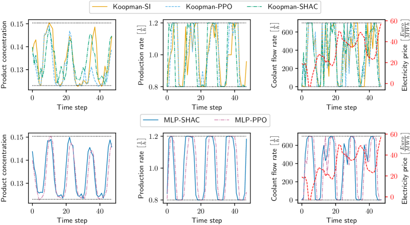
Figure 3: Comparison of the controllers. We show a randomly chosen two-day interval from the test episode. The dotted black lines represent the bounds.

We train the policies using day-ahead electricity prices from the Austrian market from March 29, 2015, to March 25, 2018 [25]. Using random seeds, we repeat the controller training ten times for each combination of policy and training algorithm (except for the Koopman-SI controller, whose Koopman model is not trained any further after SI).

All code used for training the controllers, including the hyperparameters that were used to obtain the results presented in Subsection III-C, is publicly available on GitLab. We used the Stable-Baselines3 [26] implementation of PPO but implemented our own version of SHAC following the description in [7].

III-C Results

For each type of controller trained using PPO or SHAC, we identify the controller (and the associated set of parameters) that achieved the highest average reward between two consecutive parameter updates. We test their performance and that of the Koopman-SI controller on a continuous roughly half-year-long test episode using Austrian day ahead electricity price data from March 26, 2018, to September 30, 2018 [25]. Unlike the training process, we perform this testing without exploration, i.e., we waive adding Gaussian noise to the controller output (cf. Section II-D). We initialize the test episode for each controller at the steady state of the CSTR and with empty product storage. The results are presented in Table I. We also visualize the behavior of each controller by randomly choosing a two-day interval from the test episode and plotting the product concentration $c$, the production rate $\rho$, and the coolant flow rate $F$ during this interval in Fig. 3. It can be noted that all controllers leverage the entire feasible range of the control variables and the product concentration, and that the results exhibit an intuitive inverse relationship between electricity prices and coolant flow rate. We forego including the temperature $T$ in Fig. 3 as $T$ never reaches its bounds in any of the test episodes.

TABLE I: Test results: Costs are stated relative to steady-state production cost. The percentage of control steps that result in constraint violations is given. The average size of a constraint violation is given relative to the size of the feasible range of the variable whose bound was violated.

	Cost	Constr. viols. [%]	Avg. size constr. viol.
MLP-PPO	$\bm{0.88}$	$6.34$	$9.3\cdot 10^{-3}$
MLP-SHAC	$0.90$	$0.93$	$9.8\cdot 10^{-3}$
Koopman-SI	$0.90$	$36.24$	$8.2\cdot 10^{-3}$
Koopman-PPO	$0.90$	$22.31$	$9.9\cdot 10^{-3}$
Koopman-SHAC	$0.90$	$\bm{0.39}$	$\bm{6.0\cdot 10^{-5}}$

As can be seen from Table I, Koopman-SHAC causes the fewest and also the smallest constraint violations of all tested controllers in this particular case study. MLP-PPO achieves slightly higher cost savings, but produces a much higher rate and size of constraint violations.

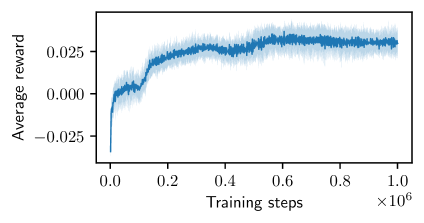
Figure 4: Learning progress in the Koopman-SHAC training runs. The dark blue line indicates the running average reward over the previous 1024 steps in the environment, averaged over all ten training runs. The light blue region indicates one standard deviation of the performance variance between the training runs.

It is noticeable that Koopman-SI and Koopman-PPO cause substantially more constraint violations than the other controllers. In the case of Koopman-SI, this is not surprising since the employed Koopman surrogate model received no end-to-end training for task-optimal performance. Here, frequent but minor constraint violations show that the controller is trying to operate at the borders of the feasible range, which is normal behavior for a predictive controller. However, in the case of Koopman-PPO the results are somewhat unsatisfactory and we observe that some training runs did not improve performance compared to Koopman-SI. Moreover, those training runs that did improve performance did not show stable convergence to high rewards. In contrast, SHAC leads to a relatively stable convergence to high rewards in our particular case study (Fig. 4). The control performance improves relatively evenly in all ten training runs without ever dropping for extended periods.

Due to the size of the case study under consideration, a detailed analysis of the training runtimes would provide little insight about the expected runtime on a control problem of more practical relevance. Therefore, we leave such an analysis for future work on larger systems.

IV Conclusion

We combine our previously published method for turning Koopman-(e)NMPC controllers into differentiable policies [4] with the policy optimization algorithm SHAC [7]. SHAC leverages derivative information from automatically differentiable simulated environments. We show that exploiting such derivative information translates to superior performance in end-to-end training of a Koopman surrogate model for eNMPC of a literature known CSTR. We also show that convergence to high control performance is fairly stable across all independent training instances. The results can be understood as a successful proof of concept. Future work should investigate the application of our method to larger mechanistic simulation models and more challenging control problems, presumably necessitating training for more iterations. Furthermore, the computational burden of backpropagation through mechanistic simulations and optimal control problems and thus the cost of each iteration is naturally linked to the size of the mechanistic simulation model, meaning that our method could become computationally intractable for very large models.

References

- [1] K. McBride and K. Sundmacher, “Overview of surrogate modeling in chemical process engineering,” Chemie Ingenieur Technik, vol. 91, no. 3, pp. 228–239, 2019.
- [2] B. Chen, Z. Cai, and M. Bergés, “Gnu-RL: A precocial reinforcement learning solution for building HVAC control using a differentiable MPC policy,” in Proceedings of the 6th ACM International Conference on Systems for Energy-Efficient Buildings, Cities, and Transportation, 2019, pp. 316–325.
- [3] S. Gros and M. Zanon, “Data-driven economic NMPC using reinforcement learning,” IEEE Transactions on Automatic Control, vol. 65, no. 2, pp. 636–648, 2019.
- [4] D. Mayfrank, A. Mitsos, and M. Dahmen, “End-to-end reinforcement learning of Koopman models for economic nonlinear MPC,” arXiv preprint arXiv:2308.01674, 2023.
- [5] A. R. Mahmood, D. Korenkevych, G. Vasan, W. Ma, and J. Bergstra, “Benchmarking reinforcement learning algorithms on real-world robots,” in Conference on Robot Learning. PMLR, 2018, pp. 561–591.
- [6] M. A. Z. Mora, M. Peychev, S. Ha, M. Vechev, and S. Coros, “Pods: Policy optimization via differentiable simulation,” in International Conference on Machine Learning. PMLR, 2021, pp. 7805–7817.
- [7] J. Xu, V. Makoviychuk, Y. Narang, F. Ramos, W. Matusik, A. Garg, and M. Macklin, “Accelerated policy learning with parallel differentiable simulation,” arXiv preprint arXiv:2204.07137, 2022.
- [8] A. Ilyas, L. Engstrom, S. Santurkar, D. Tsipras, F. Janoos, L. Rudolph, and A. Madry, “A closer look at deep policy gradients,” arXiv preprint arXiv:1811.02553, 2018.
- [9] S. Wu, L. Shi, J. Wang, and G. Tian, “Understanding policy gradient algorithms: A sensitivity-based approach,” in International Conference on Machine Learning. PMLR, 2022, pp. 24 131–24 149.
- [10] R. Islam, P. Henderson, M. Gomrokchi, and D. Precup, “Reproducibility of benchmarked deep reinforcement learning tasks for continuous control,” arXiv preprint arXiv:1708.04133, 2017.
- [11] P. Henderson, R. Islam, P. Bachman, J. Pineau, D. Precup, and D. Meger, “Deep reinforcement learning that matters,” in Proceedings of the AAAI Conference on Artificial Intelligence, vol. 32, 2018, pp. 3207–3214.
- [12] P. Henderson, J. Romoff, and J. Pineau, “Where did my optimum go?: An empirical analysis of gradient descent optimization in policy gradient methods,” arXiv preprint arXiv:1810.02525, 2018.
- [13] R. T. Q. Chen, Y. Rubanova, J. Bettencourt, and D. Duvenaud, “Neural ordinary differential equations,” Advances in Neural Information Processing Systems, vol. 31, pp. 6572–6583, 2018.
- [14] P. J. Werbos, “Backpropagation through time: what it does and how to do it,” Proceedings of the IEEE, vol. 78, no. 10, pp. 1550–1560, 1990.
- [15] Z. Huang, Y. Hu, T. Du, S. Zhou, H. Su, J. B. Tenenbaum, and C. Gan, “Plasticinelab: A soft-body manipulation benchmark with differentiable physics,” arXiv preprint arXiv:2104.03311, 2021.
- [16] B. Amos, I. Jimenez, J. Sacks, B. Boots, and J. Z. Kolter, “Differentiable MPC for end-to-end planning and control,” Advances in Neural Information Processing Systems, vol. 31, pp. 8299–8310, 2018.
- [17] A. Flores-Tlacuahuac and I. E. Grossmann, “Simultaneous cyclic scheduling and control of a multiproduct CSTR,” Industrial & Engineering Chemistry Research, vol. 45, no. 20, pp. 6698–6712, 2006.
- [18] R. S. Sutton and A. G. Barto, Reinforcement Learning: An Introduction. MIT press, 2018.
- [19] B. O. Koopman, “Hamiltonian systems and transformation in hilbert space,” Proceedings of the National Academy of Sciences, vol. 17, no. 5, pp. 315–318, 1931.
- [20] M. Korda and I. Mezić, “Linear predictors for nonlinear dynamical systems: Koopman operator meets model predictive control,” Automatica, vol. 93, pp. 149–160, 2018.
- [21] B. Lusch, J. N. Kutz, and S. L. Brunton, “Deep learning for universal linear embeddings of nonlinear dynamics,” Nature Communications, vol. 9, no. 1, pp. 1–10, 2018.
- [22] A. Paszke, S. Gross, F. Massa, A. Lerer, J. Bradbury, G. Chanan, T. Killeen, Z. Lin, N. Gimelshein, L. Antiga et al., “PyTorch: An imperative style, high-performance deep learning library,” Advances in Neural Information Processing Systems, vol. 32, pp. 8024–8035, 2019.
- [23] A. Agrawal, B. Amos, S. Barratt, S. Boyd, S. Diamond, and J. Z. Kolter, “Differentiable convex optimization layers,” Advances in Neural Information Processing Systems, vol. 32, pp. 9558–9570, 2019.
- [24] J. Schulman, F. Wolski, P. Dhariwal, A. Radford, and O. Klimov, “Proximal policy optimization algorithms,” arXiv preprint arXiv:1707.06347, 2017.
- [25] “Open Power System Data,” https://data.open-power-system-data.org/time_series/ (accessed on 2022-08-29), 2020.
- [26] A. Raffin, A. Hill, A. Gleave, A. Kanervisto, M. Ernestus, and N. Dormann, “Stable-baselines3: Reliable reinforcement learning implementations,” Journal of Machine Learning Research, vol. 22, no. 268, pp. 1–8, 2021. [Online]. Available: http://jmlr.org/papers/v22/20-1364.html