Uniqueness of static vacuum asymptotically flat black holes and equipotential photon surfaces
in $n+1$ dimensions à la Robinson

Abstract.

In this paper, we generalize to higher dimensions Robinson’s approach to proving the uniqueness of connected $(3+1)$-dimensional static vacuum asymptotically flat black hole spacetimes. In consequence, we prove geometric inequalities for connected $(n+1)$-dimensional static vacuum asymptotically flat black holes, recovering results by Agostiniani and Mazzieri. We also obtain similar geometric inequalities for connected $(n+1)$-dimensional static vacuum asymptotically flat equipotential photon surfaces and in particular photon spheres. Assuming a natural upper bound on the total scalar curvature, we recover the well-known uniqueness results for such black holes and equipotential photon surfaces. We also extend the known equipotential photon surface uniqueness results to spacetimes with negative mass. In order to replace the role of the Cotton tensor in Robinson’s proof, we introduce techniques inspired by the analysis of Ricci solitons.

Mathematics Subject Classification (2020): 83C15, 53C17, 83C57, 53C24
Keywords: Black holes, static metrics, vacuum Einstein equation, equipotential photon surfaces, photon spheres.

1. Introduction and results

Black holes are among the most intriguing objects in nature and have captured the attention of researchers since Schwarzschild provided the first non-trivial solution of Einstein’s equation of general relativity. Their properties and shape have since and continue to be thoroughly investigated. In the static case, it is well-established [23, 29, 32, 3, 28, 1, 31] that the black hole solution found by Schwarzschild constitutes the only $3+1$-dimensional asymptotically flat static vacuum spacetime with an (a priori possibly disconnected) black hole horizon arising as its inner boundary. This fact is known as “(asymptotically flat) static vacuum black hole uniqueness”; it also goes by the pictorial statement that “static vacuum (isolated) black holes have no hair”. We refer the interested reader to the reviews [20, 33] for more information.

In the higher dimensional case $n+1\geq 3+1$, the analogous fact has also been asserted; however, all proofs make extra assumptions. The proofs by Hwang [22] and by Gibbons, Ida, and Shiromizu [17] extend the method by Bunting and Masood-ul-Alam [3] allowing to deal with possibly disconnected horizons (see [6, 9] for a slightly more general version of this approach, and see [21] for a review of related results). These results rely on the rigidity case of the positive mass theorem and hence currently make a spin assumption (using Witten’s Dirac operator approach [37]) or impose an upper bound of $n+1\leq 7+1$ (using the minimal hypersurface approach by Schoen and Yau [35, 34]). Building on ideas by Simon, Raulot [31] exploits spinor techniques and thus explicitly makes a spin assumption. Instead, the proof by Agostiniani and Mazzieri [1] via potential theory, monotone functionals, and a (conformal) splitting theorem assumes connectedness of the horizon as well as an upper bound on the total scalar curvature of the (time-slice) of the horizon (see below and Section 6 for more details); their approach does not rely on the positive mass theorem. The first main goal of this paper is to demonstrate that a suitably generalized version of Robinson’s approach [32] for $n+1=3+1$ dimensions via a divergence identity (see Theorem 1.4 below) also allows to prove static vacuum black hole uniqueness for $n+1\geq 3+1$ dimensions under the same assumptions as Agostiniani and Mazzieri [1, Theorem 2.8], see Theorem 1.1 below. Our method is analytically less involved than that of [1] and also does not rely on the positive mass theorem. Moreover, we reproduce the geometric inequalities for connected horizons proved in [1, Theorem 2.8]. We impose weaker asymptotic decay assumptions than [1, Theorem 2.8], see Remark 2.3.

Theorem 1.1 (Black Hole Uniqueness).

Let $(M^{n},g,f)$ be an asymptotically flat static vacuum system of mass $m\in\mathbb{R}$ and dimension $n\geq 3$ with connected static horizon inner boundary $\partial M$. Let

(1.1) $$s_{\partial M}\mathrel{\raise 0.40903pt\hbox{\rm:}\mkern-5.2mu=}\left(\frac{|\partial M|}{|\mathbb{S}^{n-1}|}\right)^{\frac{1}{n-1}}$$

denote the surface area radius of $\partial M$, where $|\partial M|$ and $|\mathbb{S}^{n-1}|$ denote the surface area of $(\partial M,g_{\partial M})$ with respect to the induced metric $g_{\partial M}$ on $\partial M$ and of $(\mathbb{S}^{n-1},g_{\mathbb{S}^{n-1}})$, respectively. Then

(1.2) $$\frac{\left(s_{\partial M}\right)^{n-2}}{2}\sqrt{\frac{\int_{\partial M}\operatorname{R}_{\partial M}\,dS}{(n-1)(n-2)\,|\mathbb{S}^{n-1}|\left(s_{\partial M}\right)^{n-3}}}\geq m\geq\frac{\left(s_{\partial M}\right)^{n-2}}{2},$$

where $\operatorname{R}_{\partial M}$ and $dS$ denote the scalar curvature and the hypersurface area element of $\partial M$ with respect to $g_{\partial M}$, respectively. In particular, $\partial M$ satisfies

(1.3) $$\int_{\partial M}\operatorname{R}_{\partial M}dS\geq(n-1)(n-2)|\mathbb{S}^{n-1}|\left(s_{\partial M}\right)^{n-3}$$

and $(M,g,f)$ has positive mass $m>0$. Moreover, if

(1.4) $$\int_{\partial M}\operatorname{R}_{\partial M}dS\leq(n-1)(n-2)|\mathbb{S}^{n-1}|\left(s_{\partial M}\right)^{n-3}$$

then $(M,g)$ is isometric to the Schwarzschild manifold $(M^{n}_{m},g_{m})$ of mass $m$ and $f$ corresponds to $f_{m}$ under this isometry.

The last statement gives the desired black hole uniqueness result subject to a scalar curvature bound condition, see also Remark 1.3. Theorem 1.1 implies several other interesting geometric inequalities such as a static version of the Riemannian Penrose inequality, see [1] and Section 6 for more information.

Another recent direction of extending static vacuum black hole uniqueness results is to investigate uniqueness of spacetimes containing “photon spheres” (as introduced in [16]) or, more generally, “photon surfaces” (as introduced in [16, 30]). Here, photon surfaces are timelike hypersurfaces of a spacetime which “capture” null geodesics; in static spacetimes, a photon surface is called equipotential if the lapse function along it “only depends on time”, and a photon sphere if the lapse function is (fully) constant along it (as introduced in [8], see Section 2.2 and the references given there for definitions and more information). Photon surfaces are relevant in gravitational lensing and in geometric optics, i.e. for trapping phenomena, and related to dynamical stability questions for black holes.

Photon spheres were first discovered in the $3+1$-dimensional Schwarzschild spacetime and persist in its higher dimensional analog. (Equipotential) photon surfaces also naturally occur in Schwarzschild spacetimes of all dimensions and for all positive and negative masses, see [12, 14]. (Asymptotically flat) static vacuum equipotential photon surface uniqueness is fully established in $3+1$ spacetime dimensions [8, 11, 12, 10, 31]. In particular, [11, 12, 31] allow for combinations of black hole horizons and equipotential photon surfaces, assuming that all equipotential photon surface components are “outward directed”, meaning that they have “positive quasi-local mass”, see Remark 2.14. In contrast, Cederbaum, Cogo, and Fehrenbach [10] restrict to a connected, not necessarily outward directed equipotential photon surface, establishing uniqueness for the first time also in the negative (total) mass case. They generalize, exploit, and compare different techniques of proof, namely those from [23, 8, 1] and in particular Robinson’s approach [32].

In higher dimensions $n+1\geq 3+1$, the same result is established by Cederbaum and Galloway [12], building on work by Cederbaum [6, 9] which uses the positive mass theorem; hence the ensuing restrictions discussed above apply. Raulot’s spinorial approach [31] also covers higher dimensions, subject to a spin condition. The second main goal of this paper is to demonstrate that the generalized Robinson approach we derive can also be used to prove the expected uniqueness claim for connected equipotential photon surfaces, assuming the same upper bound on the total scalar curvature as in the black hole case, see Theorem 1.2 below. This generalizes the $3+1$-dimensional extension of Robinson’s approach to connected equipotential photon surfaces by Cederbaum, Cogo, and Fehrenbach [10] and also imposes weaker asymptotic decay assumptions, see Remark 2.3. Moreover, we prove similar geometric inequalities for connected equipotential photon surfaces as for black holes. Last but not least, we include the negative (total) mass case which has so far only been addressed in [10] in $3+1$ dimensions.

Theorem 1.2 (Equipotential Photon Surface Uniqueness).

Let $(M^{n},g,f)$ be an asymptotically flat static vacuum system of mass $m\in\mathbb{R}$ and dimension $n\geq 3$ with connected boundary $\partial M$ arising as a time-slice of an equipotential photon surface. Let $f_{0}>0$ denote the constant value of $f$ on $\partial M$ and assume that $f_{0}\neq 1$. If $f_{0}\in(0,1)$ then

(1.5) $$\begin{split}\frac{(1-f_{0}^{2})\left(s_{\partial M}\right)^{n-2}}{2}\,\sqrt{\frac{\left(s_{\partial M}\right)^{2}\left(\operatorname{R}_{\partial M}-\frac{n-2}{n-1}\operatorname{H}^{2}\right)}{(n-1)(n-2)(1-f_{0}^{2})}}\geq m\geq\frac{(1-f_{0}^{2})\left(s_{\partial M}\right)^{n-2}}{2}.\end{split}$$

Here, $\operatorname{R}_{\partial M}$, $\operatorname{H}$, and $s_{\partial M}$ denote the scalar curvature, the mean curvature, and the surface area radius (1.1) of $\partial M$ with respect to the induced metric $g_{\partial M}$ on $\partial M$, respectively. In particular, $\partial M$ satisfies

(1.6) $$\operatorname{R}_{\partial M}-\tfrac{n-2}{n-1}\operatorname{H}^{2}\geq\frac{(n-1)(n-2)(1-f_{0}^{2})}{\left(s_{\partial M}\right)^{2}}$$

and $(M,g,f)$ has positive mass $m>0$. If $f_{0}\in(1,\infty)$ then

(1.7) $$\begin{split}\frac{(1-f_{0}^{2})\left(s_{\partial M}\right)^{n-2}}{2}\,\sqrt{\frac{\left(s_{\partial M}\right)^{2}\left(\operatorname{R}_{\partial M}-\frac{n-2}{n-1}\operatorname{H}^{2}\right)}{(n-1)(n-2)(1-f_{0}^{2})}}\leq m\leq\frac{(1-f_{0}^{2})\left(s_{\partial M}\right)^{n-2}}{2}.\end{split}$$

In particular, $\partial M$ satisfies

(1.8) $$\operatorname{R}_{\partial M}-\tfrac{n-2}{n-1}\operatorname{H}^{2}\leq\frac{(n-1)(n-2)(1-f_{0}^{2})}{\left(s_{\partial M}\right)^{2}}$$

and $(M,g,f)$ has negative mass $m<0$. Moreover, for any $f_{0}\in(0,1)\cup(1,\infty)$, if

(1.9) $$\operatorname{R}_{\partial M}\leq\frac{(n-1)(n-2)}{\left(s_{\partial M}\right)^{2}}$$

then $(M,g)$ is isometric to the piece $[s_{\partial M},\infty)\times\mathbb{S}^{n-1}$ of the Schwarzschild manifold $(M^{n}_{m},g_{m})$ of mass $m$ and $f$ corresponds to the restriction of $f_{m}$ to $[s_{\partial M},\infty)$ under this isometry.

The last statement gives the desired equipotential photon surface uniqueness result subject to a scalar curvature bound condition, see also Remark 1.3. Theorem 1.2 implies several other interesting geometric inequalities, see [1] and Section 6.

Remark 1.3 (About Conditions (1.4) and (1.9)).

Note that (1.4) and (1.9) are equivalent in case $\operatorname{R}_{\partial M}=\text{const}$ (as it is the case for time-slices of equipotential photon surfaces, see Proposition 2.10). In dimension $n=3$, conditions (1.4) and (1.9) are of course automatically satisfied by the Gauß–Bonnet theorem. Hence Theorem 1.1 gives static vacuum black hole uniqueness in $3$ dimensions without extra assumptions (other than connectedness of the static horizon) and Theorem 1.2 gives static vacuum equipotential photon surface uniqueness in $3$ dimensions without extra assumptions (other than connectedness of the static horizon), including the negative (total) mass case.

To prove Theorems 1.1 and 1.2, we proceed as follows: First, in Section 3, we derive the following higher dimensional version of Robinson’s identity [32, Equation (2.3)], using the so-called $T$-tensor instead of the Cotton tensor $C$ Robinson uses.

Theorem 1.4 (Generalized Robinson identity).

Let $(M^{n},g,f)$, $n\geq 3$, be a static vacuum system with $0<f<1$ or $f>1$ in $M$. Then, for every $p\geq 3$ and all $c,d\in\mathbb{R}$, the generalized Robinson identity

(1.10) $$\begin{split}&\|\nabla f\|^{2}\,\operatorname{div}\left(\frac{F(f)}{f}\|\nabla f\|^{p-3}\,\nabla\|\nabla f\|^{2}+G(f)\|\nabla f\|^{p-1}\,\nabla f\right)\\ &=\|\nabla f\|^{p-3}\left[\frac{(n-2)^{2}}{(n-1)^{2}}fF(f)\|T\|^{2}\right.\\ &\quad\phantom{\|\nabla f\|^{p-3}}\quad\left.+\frac{n}{2(n-1)}\frac{F(f)}{f}\left\|\nabla\|\nabla f\|^{2}+\frac{4(n-1)}{(n-2)}\frac{f\|\nabla f\|^{2}\,\nabla f}{1-f^{2}}\right\|^{2}\right]\end{split}$$

holds almost everywhere on $M$. Here, $F,G\colon[0,1)\cup(1,\infty)\to\mathbb{R}$ are given by

(1.11) $$F(t) \mathrel{\raise 0.40903pt\hbox{\rm:}\mkern-5.2mu=}\frac{ct^{2}+d}{|1-t^{2}|^{\frac{(n-1)(p-1)}{n-2}-1}},$$

(1.12) $$G(t) \mathrel{\raise 0.40903pt\hbox{\rm:}\mkern-5.2mu=}\frac{4\left(\frac{(n-1)(p-1)}{n-2}-1\right)F(t)}{(p-1)(1-t^{2})}-\frac{4c}{(p-1)|1-t^{2}|^{\frac{(p-1)(n-1)}{n-2}-1}},$$

$\|\cdot\|$, $\nabla$, and $\operatorname{div}$ denote the tensor norm, covariant derivative, and covariant divergence with respect to $g$. The tensor $T$ is given by

(1.13) $$\begin{split}T(X,Y,Z)\mathrel{\raise 0.40903pt\hbox{\rm:}\mkern-5.2mu=}&\tfrac{(n-1)}{(n-2)}\left(\operatorname{Ric}(X,Z)\nabla_{\!Y}f-\operatorname{Ric}(Y,Z)\nabla_{\!X}f\right)\\ &-\tfrac{1}{(n-2)}\left(\operatorname{Ric}(X,\nabla f)g(Y,Z)-\operatorname{Ric}(Y,\nabla f)g(X,Z)\right),\end{split}$$

for $X,Y,Z\in\Gamma(TM)$, where $\operatorname{Ric}$ denotes the Ricci curvature tensor of $(M^{n},g)$.

Theorem 1.4 reproduces Robinson’s identity [32, (2.3)] when $n=3$, $p=3$, and $0<f<1$, and its generalization to the negative mass case by Cederbaum, Cogo, and Fehrenbach [10] when $n=3$, $p=3$, and $f>1$. It may be of independent interest, allowing to prove geometric inequalities for more general boundary geometries than the level set boundaries we are interested in in this work. As it is purely local, it may also be of use to prove related results in different asymptotic scenarios.

The $T$-tensor introduced in (1.13) is specifically adapted to the geometry of static vacuum systems, see Section 2.3. It is similar to the $D$-tensor introduced for the analysis and classification of Ricci solitons by Cao and Chen [4], inspired by Israel’s [23] and in particular Robinson’s [32] approaches to proving black hole uniqueness. The $D$-tensor was also used in [2, 5] to investigate Ricci solitons and by [25] to classify perfect fluid spaces.

As the next step in proving Theorems 1.1 and 1.2, we will exploit Theorem 1.4 to prove some important geometric inequalities on $\partial M$. These inequalities can be stated in a parametric way (Theorem 1.5), or, equivalently, as two separate inequalities (Theorem 1.6). Both versions of the geometric inequalities and their equivalence will be proven in Section 4.

Theorem 1.5 (Parametric geometric inequalities).

Let $(M^{n},g,f)$, $n\geq 3$, be an asymptotically flat static vacuum system of mass $m\in\mathbb{R}$ with connected boundary $\partial M$. Assume that $f|_{\partial M}=f_{0}$ for a constant $f_{0}\in[0,1)\cup(1,\infty)$ and that the normal derivative $\nu(f)|_{\partial M}\mathrel{=\mkern-5.2mu\raise 0.40903pt\hbox{\rm:}}\kappa$ is constant, with unit normal $\nu$ pointing towards the asymptotic end. Let $F$ and $G$ be as in Theorem 1.4 for some $p\geq 3$ and some constants $c,d\in\mathbb{R}$ satisfying $c+d\geq 0$ and $cf_{0}^{2}+d\geq 0$. Set $F_{0}\mathrel{\raise 0.40903pt\hbox{\rm:}\mkern-5.2mu=}F(f_{0})$, $G_{0}\mathrel{\raise 0.40903pt\hbox{\rm:}\mkern-5.2mu=}G(f_{0})$. Then

(1.14) $$F_{0}\,\kappa^{p-2}\int_{\partial M}\left(\operatorname{R}_{\partial M}-\tfrac{n-2}{n-1}\operatorname{H}^{2}+\|\mathring{h}\|^{2}\right)dS-G_{0}\,\kappa^{p}|\partial M|\geq\mathcal{F}^{\,c,d}_{\!p}(m),$$

and $\kappa,m>0$ if $f_{0}\in[0,1)$ and

(1.15) $$F_{0}\,|\kappa|^{p-2}\int_{\partial M}\left(\operatorname{R}_{\partial M}-\tfrac{n-2}{n-1}\operatorname{H}^{2}+\|\mathring{h}\|^{2}\right)dS-G_{0}\,|\kappa|^{p}|\partial M|\leq-\mathcal{F}^{\,c,d}_{\!p}(m)$$

and $\kappa,m<0$ if $f_{0}\in(1,\infty)$. Here, $\operatorname{R}_{\partial M}$, $\operatorname{H}$, $\mathring{h}$, and $dS$ denote the scalar curvature, the mean curvature, the trace-free part of the second fundamental form, and the area element of $\partial M$, and $|\partial M|$ and $|\mathbb{S}^{n-1}|$ denote the area of $(\partial M,g_{\partial M})$ and of $(\mathbb{S}^{n-1},g_{\mathbb{S}^{n-1}})$, respectively. The constant $\mathcal{F}^{c,d}_{p}(m)\in\mathbb{R}$ is given by

(1.16) $$\mathcal{F}^{\,c,d}_{\!p}(m) \mathrel{\raise 0.40903pt\hbox{\rm:}\mkern-5.2mu=}\frac{4(n-2)^{p}}{2^{\frac{(n-1)(p-1)}{n-2}}(p-1)}|\mathbb{S}^{n-1}|(c+d)|m|^{p-\frac{(n-1)(p-1)}{n-2}}.$$

Provided that $c,d\in\mathbb{R}$ are chosen as above, equality in (1.14) or in (1.15) holds if and only if $T=0$ as well as

(1.17) $$\nabla\|\nabla f\|^{2}+\frac{4(n-1)}{(n-2)}\frac{f\|\nabla f\|^{2}\,\nabla f}{(1-f^{2})} =0$$

hold on $M$ (unless $c=d=0$).

This can equivalently be expressed as follows.

Theorem 1.6 (Geometric inequalities).

Let $(M^{n},g,f)$, $n\geq 3$, be an asymptotically flat static vacuum system of mass $m\in\mathbb{R}$ with connected boundary $\partial M$. Assume that $f|_{\partial M}=f_{0}$ for a constant $f_{0}\in[0,1)\cup(1,\infty)$ and that $\nu(f)|_{\partial M}\mathrel{=\mkern-5.2mu\raise 0.40903pt\hbox{\rm:}}\kappa$ is constant. Then

(1.18) $$\begin{split}\frac{(1-f_{0}^{2})\left(s_{\partial M}\right)^{n-2}}{2}&\sqrt{\frac{\int_{\partial M}\left(\operatorname{R}_{\partial M}-\frac{n-2}{n-1}\operatorname{H}^{2}+\|\mathring{h}\|^{2}\right)dS}{(n-1)(n-2)(1-f_{0}^{2})|\mathbb{S}^{n-1}|\left(s_{\partial M}\right)^{n-3}}}\\ &\quad\geq m\geq\frac{(1-f_{0}^{2})\left(s_{\partial M}\right)^{n-2}}{2}.\end{split}$$

holds if $f_{0}\in[0,1)$ and

(1.19) $$\begin{split}\frac{(1-f_{0}^{2})\left(s_{\partial M}\right)^{n-2}}{2}&\sqrt{\frac{\int_{\partial M}\left(\operatorname{R}_{\partial M}-\frac{n-2}{n-1}\operatorname{H}^{2}+\|\mathring{h}\|^{2}\right)dS}{(n-1)(n-2)(1-f_{0}^{2})|\mathbb{S}^{n-1}|\left(s_{\partial M}\right)^{n-3}}}\\ &\quad\leq m\leq\frac{(1-f_{0}^{2})\left(s_{\partial M}\right)^{n-2}}{2}\end{split}$$

holds if $f_{0}\in(1,\infty)$. Equality holds on either side in each of (1.18), (1.19) if and only if $T=0$ and (1.17) hold on $M$ (unless $c=d=0$).

Theorem 1.6 may be of independent interest as it assumes much less about the properties of $\partial M$ than Theorems 1.1 and 1.2. Similar geometric inequalities may be derived from Theorem 1.4 under different asymptotic and/or inner boundary conditions.

Having established Theorem 1.6, Theorems 1.1 and 1.2 will follow via the following very general rigidity theorem which we will prove in Section 5.

Theorem 1.7 (Rigidity theorem).

Let $(M^{n},g,f)$, $n\geq 3$, be an asymptotically flat static vacuum system of mass $m\in\mathbb{R}$ with connected boundary $\partial M$. Assume that $f|_{\partial M}=f_{0}$ for a constant $f_{0}\in[0,1)\cup(1,\infty)$. Assume that $T=0$ and (1.17) hold on $M$. Then $(M,g)$ is isometric to the piece $[s_{\partial M},\infty)\times\mathbb{S}^{n-1}$ of the Schwarzschild manifold $(M^{n}_{m},g_{m})$ of mass $m$ and $f$ corresponds to the restriction of $f_{m}$ to $[s_{\partial M},\infty)$ under this isometry. In particular $\partial M$ is totally umbilic, has constant mean curvature, and is isometric to a round sphere.

Note that Theorem 1.7 makes even fewer assumptions on $\partial M$ than Theorems 1.4, 1.5 and 1.6. It could hence be of independent interest. It may also be possible to adapt it to other asymptotic scenarios.

Having completed the proofs of Theorems 1.1 and 1.2, we will then discuss some geometric implications as well as the relation to the proof of Theorem 1.1 given by Agostiniani and Mazzieri [1] in Section 6. In particular, we will define monotone functionals $\mathcal{H}^{c,d}_{p}$ along the level sets of the lapse function $f$ in the style of the functionals $U_{p}$ introduced in [1] and discuss the relation between $\mathcal{H}^{c,d}_{p}$ and $U_{p}$. This will shed some light on the relation of the two proofs.

This paper is structured as follows:

In Section 2, we introduce our notation and definitions, in particular the precise notion of asymptotic flatness we are using. We also collect some straightforward and/or well-known facts about static horizons, equipotential photon surfaces, and the $T$-tensor. In Section 3, we will give a proof of Theorem 1.4. In Section 4, we will prove Theorems 1.5 and 1.6 and show how they imply Theorems 1.1 and 1.2 upon appealing to Theorem 1.7 which we will prove in Section 5. The final Section 6 is dedicated to deducing and discussing consequences of Theorems 1.1 and 1.2, in particular to constructing monotone functionals along the level sets of the lapse function $f$ and comparing those to the monotone functionals introduced and exploited in [1].

Acknowledgements

The authors would like to thank Klaus Kröncke for helpful comments and questions. The work of Carla Cederbaum is supported by the focus program on Geometry at Infinity (Deutsche Forschungsgemeinschaft, SPP 2026). Albachiara Cogo is thankful to Universidade de Brasília and Universidade Federal de Goías, where part of this work has been carried out. Benedito Leandro was partially supported by CNPq Grant 403349/2021-4 and 303157/2022-4. João Paulo dos Santos was partially supported by CNPq Grant CNPq 315614/2021-8.

2. Preliminaries

In this section, we will collect all relevant definitions as well as some straightforward and/or well-known facts useful for the proofs of Theorems 1.1 and 1.2 and Theorems 1.4, 1.5, 1.6 and 1.7. Our sign and scaling convention for the mean curvature $\operatorname{H}$ of a smooth, oriented hypersurface of $(M,g)$ is such that the unit round sphere $\mathbb{S}^{n-1}$ in $(\mathbb{R}^{n},\delta)$ has mean curvature $\operatorname{H}=n-1$ with respect to the unit normal $\nu$ pointing towards infinity.

2.1. Static vacuum systems and asymptotic considerations

Definition 2.1 (Static vacuum systems).

A smooth Riemannian manifold $(M^{n},g)$, $n\geq 3$, is called a static system if there exists a smooth lapse function $f\colon M\rightarrow(0,+\infty)$. A static system is called a static vacuum system if it satisfies the static vacuum (Einstein) equations

(2.1) $$\nabla^{2}f =f\operatorname{Ric},$$

(2.2) $$\Delta f =0,$$

where $\nabla^{2}$ and $\Delta$ denote the Hessian and Laplacian with respect to $g$, respectively, and $\operatorname{Ric}$ denotes its Ricci curvature tensor. If $M$ has non-empty boundary $\partial M$, it is assumed that $g$ and $f$ extend smoothly to $\partial M$, with $f\geq 0$ on $\partial M$.

It follows readily from the trace of (2.1) and from (2.2) that the scalar curvature $\operatorname{R}$ of a static vacuum system $(M^{n},g,f)$ vanishes,

(2.3) $$\operatorname{R}=0.$$

It can easily be seen that the warped product static spacetime $(\mathbb{R}\times M,\overline{g}=-f^{2}dt^{2}+g)$ constructed from a static vacuum system $(M^{n},g,f)$ satisfies the vacuum Einstein equation $\overline{\operatorname{Ric}}=0$, with $\overline{\operatorname{Ric}}$ denoting the Ricci curvature tensor of $\overline{g}$. Conversely, a static spacetime $(\mathbb{R}\times M^{n},\overline{g}=-f^{2}dt^{2}+g)$ solving the vacuum Einstein equation has time-slices $\left\{t=\text{const.}\right\}$ isometric to $(M,g)$ with lapse function $f\colon M\to(0,\infty)$ such that $(M,g,f)$ is a static vacuum system.

The prime example of a static vacuum system is the $n$-dimensional Schwarzschild system $(M^{n}_{m},g_{m},f_{m})$ of mass $m>0$ and dimension $n\geq 3$, given by

(2.4) $$\begin{split}f_{m}(r)&=\sqrt{1-\frac{2m}{r^{n-2}}},\\ g_{m}&=\frac{dr^{2}}{f_{m}(r)^{2}}+r^{2}g_{\mathbb{S}^{n-1}},\end{split}$$

on $M^{n}_{m}=((2m)^{\frac{1}{n-2}},\infty)\times\mathbb{S}^{n-1}$, where $g_{\mathbb{S}^{n-1}}$ denotes the canonical metric on $\mathbb{S}^{n-1}$ and $r\in((2m)^{\frac{1}{n-2}},\infty)$ is the radial coordinate. It is well-known that by a change of coordinates (e.g. to “isotropic coordinates”), one can assert that $g_{m}$ and $f_{m}$ smoothly extend to $\partial M_{m}=\{r=(2m)^{\frac{1}{n-2}}\}\times\mathbb{S}^{n-1}$, with induced metric $g_{\partial M_{m}}=(2m)^{\frac{2}{n-2}}g_{\mathbb{S}^{n-1}}$ and $f_{m}=0$ on $\partial M_{m}$. Moreover, by another change of coordinates (e.g. to “Kruskal–Szekeres coordinates”), one can smoothly extend the associated $(n+1)$-dimensional static Schwarzschild spacetime $(\mathbb{R}\times M_{m},\overline{g}_{m}=-f_{m}^{2}dt^{2}+g_{m})$ to include (and indeed extend beyond) the boundary of $\mathbb{R}\times M_{m}$. Similarly, the $n$-dimensional Schwarzschild system of mass $m\leq 0$ is given by (2.4) on $M^{n}_{m}=(0,\infty)\times\mathbb{S}^{n-1}$; the associated spacetime cannot be extended when $m<0$ and isometrically embeds into the Minkowski spacetime when $m=0$.

We will use the following weak notion of asymptotic flatness.

Definition 2.2 (Asymptotic flatness).

A static system $(M^{n},g,f)$, $n\geq 3$, is said to be asymptotically flat of mass $m\in\mathbb{R}$ (and decay rate $\tau\geq 0$) if there exist a mass (parameter) $m\in\mathbb{R}$ as well as a compact subset $K\subset M$ and a smooth diffeomorphism $x\colon M\setminus K\longrightarrow\mathbb{R}^{n}\setminus\overline{B}$ for some open ball $B$ such that, in the coordinates $(x^{i})$ induced by the diffeomorphism $x$,

1. the metric components $g_{ij}$ satisfy the decay conditions

   (2.5) $$(x_{*}g)_{ij} =\delta_{ij}+o_{2}(|x|^{-\tau})$$

   as $|x|\rightarrow\infty$ for all $i,j\in\left\{1,\dots,n\right\}$, and

2. the lapse function $f$ can be written as

   (2.6) $$f\circ x^{-1} =f_{m}+o_{2}(|x|^{-(n-2)})=\left(1-\frac{m}{|x|^{n-2}}\right)+o_{2}(|x|^{-(n-2)})$$

   as $|x|\rightarrow\infty$.

Here and throughout the paper, for a given smooth function $\Psi\colon\mathbb{R}^{n}\rightarrow\mathbb{R}$, the notation $\Psi=o_{l}(|x|^{\alpha})$ for some $l\in\mathbb{N}$, $\alpha\in\mathbb{R}$ means that

(2.7) $$\sum_{|J|\leq l}|x|^{\alpha+|J|}|\partial^{J}\Psi|=o(1)$$

as $|x|\rightarrow\infty$. The meaning of the notation $\Psi=O_{l}(|x|^{\alpha})$ is analogous, substituting $O(1)$ by $o(1)$ in Equation 2.7. For improved readability, we will from now on mostly suppress the explicit mention of the diffeomorphism $x$ in our formulas.

Remark 2.3 (Asymptotic assumptions, decay rates).

Theorems 1.1 and 1.2 and Theorems 1.5, 1.6 and 1.7 apply for all decay rates $\tau\geq 0$, in particular for $\tau=0$, which is why we do not explicitly mention the decay rates in their statements. See also Remark 2.15 for further information on possible decay rates.

In the standard definition of asymptotic flatness for Riemannian manifolds, one usually requires stronger asymptotic conditions, namely $g_{ij}=\delta_{ij}+O_{2}(|x|^{-\frac{1}{2}-\varepsilon})$ for some $\varepsilon>0$ and integrability of the scalar curvature $\operatorname{R}$ on $M$. Under these additional assumptions, it can be seen by a standard computation that the mass parameter $m$ from (2.6) coincides with the ADM-mass of $(M,g)$. We do not appeal to any facts or properties of the ADM-mass, so we don’t need to impose such restrictions.

Our decay assumptions are also very weak when compared with the other static vacuum uniqueness results discussed in Section 1. Most of these results require that $(M,g,f)$ is asymptotic to the Schwarzschild system of mass $m$, implying standard asymptotic flatness with $\varepsilon=\frac{1}{2}$ and also faster decay of the error term in (2.6). In contrast, [1, 10] make the same assumption on the decay of $f$ as we make in (2.6). Moreover, in [1] (and consequently in its application in [10] for $n=3$ spatial dimensions), it is assumed that $\tau=\frac{n-2}{2}$. It is however conceivable that our asymptotic decay assumption could be boot-strapped to stronger decay assertions as for example in [24], using the static vacuum equations (2.1) and (2.2).

It is well-known and straightforward to see that the Schwarzschild system $(M^{n}_{m},g_{m},f_{m})$ of mass $m$ is asymptotically flat of mass $m$ for any decay rate $\tau\geq 0$. To see this, one switches from the spherical polar coordinates $r$ and $\eta\in\mathbb{S}^{n-1}$ to the canonically associated Cartesian coordinates $x=r\eta$ outside a suitable ball.

The following remark will be useful for our strategy of proof, in particular for Theorem 1.5, where we will use it when applying the divergence theorem on $M$, and for Theorem 1.7, where we will use it to properly study the level set flow of $f$ and conclude isometry to a Schwarzschild system.

Remark 2.4 (Completeness).

Asymptotically flat static systems $(M^{n},g,f)$, $n\geq 3$, with boundary $\partial M$ are necessarily metrically and geodesically complete (up to the boundary $\partial M$) with at most finitely many boundary components, see for example [13, Appendix]. Moreover, the connected components of $\partial M$ are necessarily all closed, see for example [13, Appendix]. Here, to be geodesically complete up to the boundary means that any geodesic $\gamma\colon I\to M$ which is not defined on all of $\mathbb{R}$, $I\neq\mathbb{R}$, can be smoothly extended to a geodesic $\widehat{\gamma}\colon J\to M\cup\partial M$ such that either $J=\mathbb{R}$ or $J=[a,\infty)$, $J=(-\infty,b]$, or $J=[a,b]$ for some $a,b\in\mathbb{R}$ such that $\widehat{\gamma}(a),\widehat{\gamma}(b)\in\partial M$ (if applicable).

We will later need the following consequences of our asymptotic assumptions which we formulate for general decay rate $\tau\geq 0$ for convenience of the reader.

Lemma 2.5 (Asymptotics).

Let $(M^{n},g,f)$, $n\geq 3$, be an asymptotically flat static system of mass $m\in\mathbb{R}$ and decay rate $\tau\geq 0$ with respect to a diffeomorphism $x\colon M\setminus K\longrightarrow\mathbb{R}^{n}\setminus\overline{B}$ and denote the induced coordinates by $(x^{i})$. Then, for $i,j=1,\dots,n$, we have

$$(\nabla f)^{i} =(\nabla_{\!m}f_{m})^{i}+o_{1}(|x|^{-(n-1)})=\frac{(n-2)\,mx^{i}}{|x|^{n}}+o_{1}(|x|^{-(n-1)}),$$

$$\|\nabla f\|^{2} =\|\nabla_{\!m}f_{m}\|^{2}_{m}+o_{1}(|x|^{-2(n-1)})=\frac{(n-2)^{2}\,m^{2}}{|x|^{2(n-1)}}+o_{1}(|x|^{-2(n-1)}),$$

$$\nabla^{2}_{ij}f =(\nabla^{2}_{\!m})_{ij}f_{m}+o_{0}(|x|^{-n})=\frac{(n-2)m\delta_{ij}}{|x|^{n}}-\frac{n(n-2)mx_{i}x_{j}}{|x|^{n+2}}+o_{0}(|x|^{-n}),$$

$$\|\nabla^{2}f\|^{2} =\|\nabla_{\!m}^{2}f_{m}\|^{2}_{m}+o_{0}(|x|^{-2n})=\frac{n(n-1)(n-2)^{2}\,m^{2}}{|x|^{2n}}+o_{0}(|x|^{-2n}),$$

$$\nabla^{i}\|\nabla f\|^{2} =\nabla^{i}_{\!m}\|\nabla_{\!m}f_{m}\|^{2}_{m}+o_{0}(|x|^{-(2n-1)})=-\frac{2(n-1)(n-2)^{2}\,m^{2}x^{i}}{|x|^{2n}}+o_{0}(|x|^{-(2n-1)}),$$

$$\|\nabla\|\nabla f\|^{2}\|^{2} =\|\nabla_{\!m}\|\nabla_{m}f_{m}\|^{2}_{m}\|^{2}_{m}+o_{0}(|x|^{-2(2n-1)}),$$

$$\operatorname{Ric}(\nabla f,\nabla f) =\operatorname{Ric}_{m}(\nabla_{\!m}f_{m},\nabla_{\!m}f_{m})+o_{0}(|x|^{-(\tau+2n)})=o_{0}(|x|^{-(\tau+2n)})$$

as $|x|\to\infty$. Here, $\nabla$ and $\|\cdot\|$ denote the connection and tensor norm with respect to $g$ and $\nabla_{\!m}$, $\|\cdot\|_{m}$, and $\operatorname{Ric}_{m}$ denote the connection, tensor norm, and Ricci tensor with respect to $g_{m}$, respectively. Furthermore, let $r>0$ be such that $B_{r}\mathrel{\raise 0.40903pt\hbox{\rm:}\mkern-5.2mu=}\left\{x\in\mathbb{R}^{n}\,:\,|x|<r\right\}\supset\overline{B}$ and let $\nu$ denote the unit normal to $x^{-1}(\partial B_{r})$ pointing towards the asymptotically flat end and let $\operatorname{H}$ denote the mean curvature of $x^{-1}(\partial B_{r})$ with respect to $\nu$. Then

(2.8) $$\nu^{i} =\frac{x^{i}}{|x|}+o(|x|^{-\tau}),$$

(2.9) $$\operatorname{H} =\frac{n-1}{|x|}+o(|x|^{-1-\tau})$$

as $|x|\to\infty$. Now let $u,v,u_{0},v_{0}\colon M\setminus K\to\mathbb{R}$ be continuous functions such that $u=u_{0}+o(|x|^{-(n-1)})$, $u_{0}=O(|x|^{-(n-1)})$, $v=v_{0}+o(|x|^{-n})$, and $v_{0}=O(|x|^{-n})$ as $|x|\to\infty$. Then

(2.10) $$\int_{x^{-1}(\partial B_{r})}u\,dS =\int_{\partial B_{r}}(u_{0}\circ x^{-1})\,dS_{\delta}+o(1),$$

(2.11) $$\int_{x^{-1}(\mathbb{R}^{n}\setminus\overline{B_{r}})}v\,dV =\int_{\mathbb{R}^{n}\setminus\overline{B_{r}}}(v_{0}\circ x^{-1})\,dV_{\delta}+o(1)$$

as $r\to\infty$, where $dS$ and $dS_{\delta}$ denote the area elements induced on $x^{-1}(\partial B_{r})$ and $\partial B_{r}$ and $dV$ and $dV_{\delta}$ denote the volume elements induced on $x^{-1}(\mathbb{R}^{n}\setminus\overline{B_{r}})$ and $\mathbb{R}^{n}\setminus\overline{B}_{r}$ by $g$ and $\delta$, respectively. In particular, $v$ is integrable on $x^{-1}(\mathbb{R}^{n}\setminus\overline{B}_{r})$ with respect to $dV$.

Proof.

The claims in Lemma 2.5 follow from straightforward computations. For addressing (2.8), (2.10), and (2.11), let $(r,\theta^{J})_{J=1}^{n-1}$ be standard polar coordinates for $\mathbb{R}^{n}$ so that $(\partial_{\theta^{K}})^{i}=O_{\infty}(|x|)$ as $|x|\to\infty$ and $\delta_{IJ}=r^{2}(g_{\mathbb{S}^{n-1}})_{IJ}$. Here and in what follows, we use the convention that capital latin indices $I,J,K,\dots=1,\dots,n-1$ label the polar coordinates $(\theta^{K})$, while small latin indices $i,j,k,\dots=1,\dots,n$ label the Cartesian coordinates $(x^{i})$ as before.

For $\nu$, we make the ansatz

$$\nu^{i} =(1+\lambda)\frac{x^{i}}{|x|}-\delta^{ij}(g_{jk}-\delta_{jk})\frac{x^{k}}{|x|}+\mu^{L}(\partial_{\theta^{L}})^{i}$$

for $\lambda,\mu^{L}\in C^{\infty}(\mathbb{R}^{n}\setminus B_{r})$, $L=1,\dots,n-1$. Then for $K,L=1,\dots,n-1$, we compute

$$0=g(\nu,\partial_{\theta^{K}}) =-(g_{ij}-\delta_{ij})\frac{x^{i}}{|x|}(\partial_{\theta^{K}})^{j}+\mu^{L}|x|^{2}\,(g_{\mathbb{S}^{n-1}})_{KL}+(g_{ij}-\delta_{ij})\nu^{i}(\partial_{\theta^{K}})^{j}$$

$$=\mu^{L}|x|^{2}\left((g_{\mathbb{S}^{n-1}})_{KL}+o(|x|^{-\tau})\right)+\lambda\cdot o(|x|^{-\tau+1})+o(|x|^{-2\tau+1}),$$

$$1=\;\,g(\nu,\nu)\;\, =(1+\lambda)^{2}(1+o(|x|^{-\tau}))+\mu^{L}\cdot o(|x|^{-\tau+1})+(1+\lambda)\cdot o(|x|^{-\tau})$$

$$\quad+\mu^{K}\mu^{L}|x|^{2}\left((g_{\mathbb{S}^{n-1}})_{KL}+o(|x|^{-\tau})\right)+(1+\lambda)\mu^{L}\cdot o(|x|^{-\tau+1})+o(|x|^{-2\tau})$$

as $|x|\to\infty$. We rewrite the first equation as

(2.12) $$\mu^{L} =\lambda\cdot o(|x|^{-(\tau+1)})+o(|x|^{-(2\tau+1)})$$

and plug this into the second equation, obtaining $1=(1+\lambda)^{2}+o(r^{-\tau})+\lambda\cdot o(r^{-\tau})+\lambda^{2}\cdot o(r^{-\tau})$ and hence by Taylor’s formula, this quadratic equation has the two solutions $\lambda_{1}=o(|x|^{-\tau})$ and $\lambda_{2}=-2+o(|x|^{-\tau})$ as $|x|\to\infty$. As we are interested in finding the normal pointing towards $|x|\to\infty$, we can exclude $\lambda_{2}$ and obtain $\lambda=o(|x|^{-\tau})$ as desired. Combining this with (2.12), we find $\mu^{L}=o(|x|^{-(2\tau+1)})$ for $L=1,\dots,n-1$ as $|x|\to\infty$. This proves (2.8).

For (2.9), we compute as above that the components of the inverse induced metric $(\sigma^{IJ})$ on $x^{-1}(\partial B_{r})$ satisfy $\sigma^{IJ}=\frac{1}{|x|^{2}}(g_{\mathbb{S}^{n-1}})^{IJ}+o(|x|^{-\tau-2})$ as $|x|\to\infty$, while the components of the inverse metric satisfy $g^{rr}=1+o_{2}(|x|^{-\tau})$, $g^{rI}=o_{2}(|x|^{-\tau-1})$, $g^{IJ}=\frac{1}{|x|^{2}}(g_{\mathbb{S}^{n-1}})^{IJ}+o_{2}(|x|^{-\tau-2})$ as $|x|\to\infty$. From this, one finds that the Christoffel symbols of $g$ behave as

$$\Gamma_{IJ}^{r} =-|x|(g_{\mathbb{S}^{n-1}})_{IJ}+o(|x|^{1-\tau}),$$

$$\Gamma_{IJ}^{K} =o(|x|^{-\tau})$$

as $|x|\to\infty$ and thus, using (2.8), we obtain

$$\operatorname{H} =-\sigma^{IJ}g(\nabla_{I}\partial_{J},\nu)=\frac{n-1}{|x|}+o(|x|^{-1-\tau})$$

as $|x|\to\infty$ as claimed. Next, for (2.11), we note that

$$\sqrt{\operatorname{det}\left(g_{ij}\right)} =\sqrt{\operatorname{det}\left(\delta_{ij}+o(|x|^{-\tau})\right)}=1+o(|x|^{-\tau})$$

as $|x|\to\infty$ by Taylor’s formula. Hence

$$\int_{x^{-1}(\mathbb{R}^{n}\setminus\overline{B_{r}})}v\,dV =\int_{\mathbb{R}^{n}\setminus\overline{B_{r}}}(v\circ x^{-1})\sqrt{\operatorname{det}\left(g_{ij}\right)}\,dx^{1}\cdot\dots\cdot dx^{n}$$

$$=\int_{\mathbb{R}^{n}\setminus\overline{B_{r}}}(v\circ x^{-1})\left(1+o(|x|^{-\tau})\right)dx^{1}\cdot\dots\cdot dx^{n}$$

$$=\int_{\mathbb{R}^{n}\setminus\overline{B_{r}}}(v_{0}\circ x^{-1})\left(1+o(|x|^{-\tau})\right)dV_{\delta}+\int_{\mathbb{R}^{n}\setminus\overline{B_{r}}}o(|x|^{-n})\,dV_{\delta}$$

$$=\int_{\mathbb{R}^{n}\setminus\overline{B_{r}}}(v_{0}\circ x^{-1})\,dV_{\delta}+\int_{\mathbb{R}^{n}\setminus\overline{B_{r}}}o(|x|^{-n})\,dV_{\delta}$$

$$=\int_{\mathbb{R}^{n}\setminus\overline{B_{r}}}(v_{0}\circ x^{-1})dV_{\delta}+o(1)$$

as $|x|\to\infty$, where we have used the decay assumption on $v$ and $v_{0}$ in the third and second to last, and the $L^{\infty}$-$L^{1}$-Hölder inequality in the last step.

Finally, for (2.10), we argue as before and compute

$$\sqrt{\operatorname{det}\left(g_{IJ}\right)} =\sqrt{\operatorname{det}\left(r^{2}(g_{\mathbb{S}^{n-1}})_{IJ}+o(|x|^{-\tau+2})\right)}$$

$$=r^{n-1}\sqrt{\operatorname{det}\left((g_{\mathbb{S}^{n-1}})_{IJ}+o(|x|^{-\tau})\right)}$$

$$=r^{n-1}\sqrt{\operatorname{det}\left((g_{\mathbb{S}^{n-1}})_{IJ}\right)}\sqrt{\operatorname{det}\left(\delta_{KL}+((g_{\mathbb{S}^{n-1}})^{-1})_{KL}\cdot o(|x|^{-\tau})\right)}$$

$$=r^{n-1}\sqrt{\operatorname{det}\left((g_{\mathbb{S}^{n-1}})_{IJ}\right)}\left(1+o(|x|^{-\tau})\right)$$

as $|x|\to\infty$ by the algebraic properties of the determinant and by Taylor’s formula. Arguing as before and using the decay assumption on $u$, this implies

$$\int_{x^{-1}(\partial B_{r})}u\,dS =\int_{\partial B_{r}}(u\circ x^{-1})\sqrt{\operatorname{det}\left(g_{IJ}\right)}\,d\theta^{1}\cdot\dots\cdot d\theta^{n-1}$$

$$=\int_{\partial B_{r}}(u\circ x^{-1})\,r^{n-1}\sqrt{\operatorname{det}\left((g_{\mathbb{S}^{n-1}})_{IJ}\right)}\left(1+o(|x|^{-\tau})\right)d\theta^{1}\cdot\dots\cdot d\theta^{n-1}$$

$$=\int_{\partial B_{r}}(u\circ x^{-1})\left(1+o(|x|^{-\tau})\right)dS_{\delta}$$

$$=\int_{\partial B_{r}}(u_{0}\circ x^{-1})\left(1+o(|x|^{-\tau})\right)dS_{\delta}+\int_{\partial B_{r}}o(|x|^{-(n-1)})\,dS_{\delta}$$

$$=\int_{\partial B_{r}}(u_{0}\circ x^{-1})\,dS_{\delta}+o(1)$$

as $|x|\to\infty$. This completes the proof. ∎

Remark 2.6 (Choice of normal, regular boundary, tensor norm).

Let $(M^{n},g,f)$, $n\geq 3$, be an asymptotically flat static vacuum system of mass $m$ and decay rate $\tau\geq 0$ with connected boundary $\partial M$. Let $\nu$ denote the unit normal to $\partial M$ pointing towards the asymptotically flat end. Now assume first that $f|_{\partial M}=f_{0}$ for some $f_{0}\in[0,1)$. Then since $f$ is harmonic by (2.2), the maximum principle ensures that

(2.13) $$0\leq f_{0}<f<1$$

holds on $M$. Moreover, by the Hopf lemma, we can deduce that $\nu(f)=\|\nabla f\|>0$ on $\partial M$, implying that $\partial M$ is a regular level set of $f$. Thus

(2.14) $$\nu =\frac{\nabla f}{\|\nabla f\|},$$

where here and in what follows, $\|\cdot\|$ denotes the tensor norm induced by $g$ and we slightly abuse notation and denote the gradient of $f$ by $\nabla f$. Next assume that $f|_{\partial M}=f_{0}$ for some $f_{0}>1$. The same arguments imply that

(2.15) $$f_{0}>f>1$$

holds on $M$ and

(2.16) $$\nu =-\frac{\nabla f}{\|\nabla f\|}.$$

When studying (regular) level sets $\{f=f_{0}\}$ of $f$, we will also use the unit normal $\nu$ pointing towards infinity, so that (2.14) respectively (2.16) hold when $f_{0}\in(0,1)$ respectively $f_{0}\in(1,\infty)$. Finally, assume that $f|_{\partial M}=1$. Then by the maximum principle, $f\equiv 1$ holds on $M$.

2.2. Static horizons and equipotential photon surfaces

Static (black hole) horizons and their surface gravity are defined as follows. For simplicity, we will restrict our attention to connected static horizons already here.

Definition 2.7 (Static horizons).

Let $(M^{n},g,f)$, $n\geq 3$, be a static system with connected boundary $\partial M$. We say that $\partial M$ is a static (black hole) horizon if $f|_{\partial M}=0$.

In fact, static horizons as defined above can be seen to be Killing horizons in the sense that the static Killing vector field $\partial_{t}$ smoothly extends to the (extension to the) boundary of the static spacetime $(\mathbb{R}\times M,\overline{g}=-f^{2}dt^{2}+g)$ but at the same time degenerates along this boundary, namely $-f^{2}=\overline{g}(\partial_{t},\partial_{t})\to 0$. The standard example of a static system with a static horizon is the Schwarzschild system $(M^{n}_{m},g_{m},f_{m})$ of mass $m>0$.

Let us now collect some important properties of static horizons in static vacuum systems.

Remark 2.8 (Surface gravity, horizons are totally geodesic).

It is a well-known and straightforward consequence of (2.1) that static horizons in static vacuum systems are totally geodesic and in particular minimal surfaces. Moreover, using again (2.1), one computes that

(2.17) $$\nabla\|\nabla f\|^{2} =2f\operatorname{Ric}(\nabla f,\cdot)$$

which manifestly vanishes on a static horizon $\partial M$. This implies that the surface gravity $\kappa$ defined by

(2.18) $$\kappa\mathrel{\raise 0.40903pt\hbox{\rm:}\mkern-5.2mu=}\nu(f)|_{\partial M}$$

for some unit normal along $\partial M$ is constant on the static horizon $\partial M$. Combined with Remark 2.6, this shows that the surface gravity of a (connected) static horizon in an asymptotically flat static vacuum system is necessarily non-vanishing, $\kappa\neq 0$ and positive when one chooses $\nu$ to point to infinity. This fact is sometimes expressed as saying that such static horizons are “non-degenerate”.

Next, let us recall the definition and properties of equipotential photon surfaces and of photon spheres, the central objects studied in Theorem 1.2. We will be very brief as we will only need specific properties and refer the interested reader to [12, 14] for more information and references. In particular, we will assume that all photon surfaces are necessarily connected for simplicity of the exposition and as we will only study connected photon surfaces in this paper, anyway. It will temporarily be more convenient to think about static spacetimes rather than static systems.

Definition 2.9 ((Equipotential) photon surface, photon sphere).

A smooth, timelike, embedded, and connected hypersurface in a smooth Lorentzian manifold is called a photon surface if it is totally umbilic. A photon surface $P^{n}$ in a static spacetime $(\mathbb{R}\times M^{n},\overline{g}=-f^{2}dt^{2}+g)$ is called equipotential if the lapse function $f$ of the spacetime is constant along each connected component of each time-slice $\Sigma^{n-1}(t)\mathrel{\raise 0.40903pt\hbox{\rm:}\mkern-5.2mu=}P^{n}\,\cap\left(\{t\}\times M^{n}\right)$ of the photon surface. An equipotential photon surface is called a photon sphere if the lapse function $f$ is constant (in space and time) on $P^{n}$.

It is well-known that the (exterior) Schwarzschild spacetime of mass $m>0$ (i.e., the spacetime associated to the Schwarzschild system $(M_{m}^{n},g_{m},f_{m})$ of mass $m>0$) possesses a photon sphere at $r=(nm)^{\frac{1}{n-2}}$. Moreover, it follows from a combination of results by Cederbaum and Galloway [12, Theorem 3.5, Proposition 3.18] and by Cederbaum, Jahns, and Vičánek Martínez [14, Theorems 3.7, 3.9, and 3.10] that all Schwarzschild spacetimes possess very many equipotential photon surfaces. In particular, every sphere $\mathbb{S}^{n-1}(r)\subset M^{n}_{m}$ arises as a time-slice of an equipotential photon surface. On the other hand, no other closed hypersurfaces of $(M^{n}_{m},g_{m},f_{m})$ arise as time-slices of equipotential photon surfaces by [12, Corollary 3.9].

Let us now move on to study the intrinsic and extrinsic geometry of time-slices of equipotential photon spheres. Time-slices of equipotential photon surfaces and in particular of photon spheres have the following useful properties.

Proposition 2.10 ([14, Proposition 5.5]).

Let $(M^{n},g,f)$, $n\geq 3$, be an asymptotically flat static vacuum system and let $\partial M$ be a time-slice of an equipotential photon surface with $f=f_{0}$ on $\partial M$ for some constant $f_{0}>0$, $f_{0}\neq 1$. Then $\partial M$ is totally umbilic in $(M,g)$, has constant scalar curvature $\operatorname{R}_{\partial M}$, constant mean curvature $\operatorname{H}$, and constant $\kappa\mathrel{\raise 0.40903pt\hbox{\rm:}\mkern-5.2mu=}\nu(f)|_{\partial M}$, related by the equipotential photon surface constraint

(2.19) $$\operatorname{R}_{\partial M} =\frac{2\kappa\operatorname{H}}{f_{0}}+\frac{n-2}{n-1}\operatorname{H}^{2}.$$

Here, we are using that $\kappa=\nu(f)|_{\partial M}\neq 0$ by Remark 2.6.

Proposition 2.11 ([11, Lemma 2.6], [14, Theorem 5.22]).

In the setting of Proposition 2.10, we have $\operatorname{H}>0$.

In fact, both [11, Lemma 2.6] and [14, Theorem 5.22] assume stronger asymptotic decay conditions than we do, and in addition assume $\nu(N)>0$ resp. $\operatorname{H}\nu(N)>0$ on $\partial M$. As $\partial M$ is connected here, neither of the second assumptions are needed to conclude as can be seen in the corresponding proofs, as these conditions are needed to handle potential other boundary components only. Concerning the asymptotic decay assumptions, it suffices to note that our decay assumptions imply that large coordinate spheres have positive mean curvature by Lemma 2.5.

Remark 2.12.

Formally taking the limit of the equipotential photon surface constraint (2.19) as $f_{0}\searrow 0$, one recovers the twice contracted Gauss equation

$$\operatorname{R}_{\partial M} =-\frac{2\operatorname{Ric}(\nu,\nu)\kappa}{\|\nabla f\|}=-2\operatorname{Ric}(\nu,\nu),$$

with $\kappa$ denoting the surface gravity of the static horizon $\{f_{0}=0\}$. To see this, one uses the well-known fact that $\operatorname{H}=-\frac{\nabla^{2}f(\nu,\nu)}{\|\nabla f\|}$ on regular level sets of $f$ (see also (5.3) in the proof of Theorem 1.7), the static vacuum equation (2.1), and (2.3). In particular, the first term $\frac{2H\kappa}{f_{0}}$ of (2.19) remains well-defined in the case $f_{0}=0$.

Lemma 2.13 (Smarr formula).

Let $(M^{n},g,f)$, $n\geq 3$, be an asymptotically flat static vacuum system with mass $m\in\mathbb{R}$. Then the Smarr formula

(2.20) $$\int_{\{f=z\}}\nu(f)\,dS =(n-2)|\mathbb{S}^{n-1}|\,m$$

holds for every regular, connected level set $\{f=z\}$ of $f$, where $z\geq 0$ is a constant. Here, $|\mathbb{S}^{n-1}|$ denotes the area of $(\mathbb{S}^{n-1},g_{\mathbb{S}^{n-1}})$ and $\nu$ denotes the unit normal to $\{f=z\}$. Moreover, if $(M,g,f)$ has a connected boundary $\partial M$ then

(2.21) $$\int_{\partial M}\nu(f)\,dS =(n-2)|\mathbb{S}^{n-1}|\,m.$$

Furthermore, if in addition $f|_{\partial M}=f_{0}$ for some $f_{0}\geq 0$ then $m>0$ when $f_{0}\in[0,1)$, $m=0$ when $f_{0}=1$, and $m<0$ when $f_{0}>1$. In particular, if $\partial M$ is a static horizon or a time-slice of an equipotential photon surface with $f_{0}<1$ resp. $f_{0}>1$ then $m>0$ resp. $m<0$.

Remark 2.14 (Quasi-local mass, outward directed equipotential photon surfaces, and why we avoid the zero mass case).

The Smarr formula (2.21) allows one to define a quasi-local mass for $\partial M$ by expressing $m$ in terms of the other quantities in (2.21) (see e.g. [7]). Lemma 2.13 hence states that said quasi-local mass of a connected boundary $\partial M$ coincides with the asymptotic mass parameter $m$ of the static system. Furthermore, it informs us that if $f=f_{0}$ on $\partial M$ for some constant $f_{0}\geq 0$, then the sign/vanishing of the mass $m$ is fixed by the value of $f_{0}$. This allows to refer to the case $f_{0}\in[0,1)$ as the positive mass case, to $f_{0}=0$ as the zero mass case, and to the case $f_{0}\in(1,\infty)$ as the negative mass case, respectively. It also explains why we avoid the zero mass case in this paper altogether: If $f_{0}=1$, Remark 2.6 informs us that $f\equiv 1$ on $M$ and thus $(M,g)$ is necessarily Ricci-flat by (2.1). In dimension $n=3$, this implies that $(M,g)$ is indeed flat; one can conclude that it isometric to Euclidean space without a ball using the asymptotically flatness with decay rate $\tau\geq 0$, without assuming any additional properties (see [10]). In higher dimensions, proving a similar statement is a problem of a different nature, which is going to be addressed elsewhere.

As briefly touched upon in Section 1, the existing static vacuum uniqueness results for equipotential photon surfaces all assume that those are outward directed, meaning that $\kappa=\nu(f)|_{\partial M}>0$. In view of Lemma 2.13, this corresponds to a restriction to the positive (quasi-local) mass case.

Proof of Lemma 2.13.

The fact that the left-hand side of (2.20) is independent of the value of $z$ is a direct consequence of (2.2) and the divergence theorem. To see that the constants on the right-hand sides of (2.20), (2.21) equal $(n-2)|\mathbb{S}^{n-1}|\,m$, one argues as follows, using the notation from Lemma 2.5. First, $\nu(f)=\frac{(n-2)m}{|x|^{n-1}}+o(|x|^{-(n-1)})$ as $|x|\to\infty$ by Lemma 2.5 and (2.8). Hence $u\mathrel{\raise 0.40903pt\hbox{\rm:}\mkern-5.2mu=}\nu(f)$, $u_{0}\mathrel{\raise 0.40903pt\hbox{\rm:}\mkern-5.2mu=}\frac{(n-2)m}{|x|^{n-1}}$ are suitable functions for the application of (2.10). Then, by (2.2) and the divergence theorem, we get

$$\int_{\partial M}\nu(f)\,dS =-\int_{\{p\in M\,:\,|x|(p)<r\}}\Delta f\,dV+\int_{x^{-1}(\partial B_{r})}\nu(f)\,dS=\int_{x^{-1}(\partial B_{r})}\nu(f)\,dS$$

$$=\int_{\partial B_{r}}(u_{0}\circ x^{-1})\,dS_{\delta}+o(1)=(n-2)m\int_{\partial B_{r}}\frac{1}{|x|^{n-1}}\,dS_{\delta}+o(1)$$

$$=(n-2)|\mathbb{S}^{n-1}|\,m+o(1)$$

as $r=|x|\to\infty$, where $dV$ denotes the volume element on $M$. This proves (2.21). In particular, if $f_{0}=1$, Remark 2.6 tells us that $f=1$ on $M$ and hence there are no regular level sets of $f$ and no claim about (2.20). The asymptotic formula for $\nu(f)=0$ directly shows that $m=0$. If $f_{0}\neq 1$, regular level sets can exist and (2.20) then follows precisely as (2.21), up to a sign in front of the volume integral over $\triangle f$ if $z>1$, and with the domain of said volume integral taking the form $\{p\in M\,:\,f(p)>z,\,|x|(p)<r\}$ if $0\leq z<1$ and the form $\{p\in M\,:\,f(p)<z,\,|x|(p)<r\}$ if $z>1$ in view of Remark 2.6. The remaining claims are direct consequences of the Smarr formula and of Remark 2.6, via Proposition 2.10. ∎

Remark 2.15 (Admissible decay rates).

In Definition 2.2, we have allowed the decay rate $\tau\geq 0$ to be arbitrary. In the static vacuum setting, $\tau\geq n-2$ implies that $m=0$ via Lemma 2.13, arguing as in the proof of Lemma 2.5, hence our assumption (2.6) effectively restrict the range of the decay rate to $\tau<n-2$. As we only treat $\tau=0$ in this paper, this doesn’t affect us.

2.3. The tensor $T$ and its properties

In this section we will discuss properties of the $T$-tensor introduced in (1.13) which will be essential for establishing our results. Remember that, for a Riemannian manifold $(M^{n},\,g),$ $n\geq 3,$ the Weyl tensor $W$ is defined as

(2.22) $$W \mathrel{\raise 0.40903pt\hbox{\rm:}\mkern-5.2mu=}\operatorname{Rm}-\frac{1}{n-2}\left(\operatorname{Ric}-\frac{\operatorname{R}}{2}g\right)\mathbin{\bigcirc\mspace{-15.0mu}\wedge\mspace{3.0mu}}g-\frac{\operatorname{R}}{2n(n-1)}g\mathbin{\bigcirc\mspace{-15.0mu}\wedge\mspace{3.0mu}}g,$$

where $\operatorname{Rm}$ stands for the Riemann curvature operator of $(M,g)$, and $\mathbin{\bigcirc\mspace{-15.0mu}\wedge\mspace{3.0mu}}$ denotes the Kulkarni–Nomizu product. Moreover, the Cotton tensor $C$ of $(M,g)$ is given by

(2.23) $$\begin{split}C(X,Y,Z)&\mathrel{\raise 0.40903pt\hbox{\rm:}\mkern-5.2mu=}(\nabla_{X}\operatorname{Ric})(Y,Z)-(\nabla_{Y}\operatorname{Ric})(X,Y)\\ &\quad-\frac{1}{2(n-1)}\left((\nabla_{X}\operatorname{R})g(Y,Z)-(\nabla_{Y}\operatorname{R})g(X,Z)\right)\end{split}$$

for $X,Y,Z\in\Gamma(TM)$. It is well-known that $W$ vanishes for $n=3$, while for $n\geq 4$, $W$ and $C$ are related via

(2.24) $$C =-\frac{(n-2)}{(n-3)}(\nabla_{E_{i}}\!W)(\cdot,\cdot,\cdot,E_{j})\delta^{ij}$$

for any local orthonormal frame $\left\{E_{i}\right\}_{i=1}^{n}$ of $M$.

For $n=3$, it is well-known that the Cotton tensor detects (local) conformal flatness in the sense that $C=0$ if and only if $(M^{3},g)$ is locally conformally flat. The same holds true for the Weyl tensor when $n\geq 4$.

The $T$-tensor of a Riemannian manifold $(M^{n},g)$, $n\geq 3$, carrying a smooth function $f\colon M\to\mathbb{R}$ is given by (1.13). Due to the symmetry of the Ricci tensor, $T$ is antisymmetric in its first two entries. By a straightforward algebraic computation, its squared norm can be computed to be

(2.25) $$\|T\|^{2} =\frac{2(n-1)}{(n-2)^{2}}\left[(n-1)\|\operatorname{Ric}\|^{2}\,\|\nabla f\|^{2}-n\|\operatorname{Ric}(\nabla f,\cdot)\|^{2}+2\operatorname{R}\operatorname{Ric}(\nabla f,\nabla f)\right].$$

In particular, if $(M^{n},g,f)$, $n\geq 3$, is a static vacuum system, the last term in (2.25) vanishes by (2.3). It is interesting to note the following relation between the Weyl, the Cotton, and the $T$-tensor.

Lemma 2.16 (Relation between $W$, $C$, and $T$).

Let $(M^{n},g,f)$, $n\geq 3$, be a static vacuum system. Then

$$fC =W(\cdot,\cdot,\cdot,\nabla f)+T$$

holds on $M$.

Proof.

For simplicity, we will use abstract index notation in this proof. First, taking the covariant derivative of (2.1), we have

$$\nabla_{i}\nabla_{j}\nabla_{k}f =\nabla_{i}f\operatorname{Ric}_{jk}+f\nabla_{i}\operatorname{Ric}_{jk}.$$

Next, from the Ricci equation we get that

$$\operatorname{Ric}_{jk}\nabla_{i}f-\operatorname{Ric}_{ik}\nabla_{j}f+f\left(\nabla_{i}\operatorname{Ric}_{jk}-\nabla_{j}\operatorname{Ric}_{ik}\right) =\nabla_{i}\nabla_{j}\nabla_{k}f-\nabla_{j}\nabla_{i}\nabla_{k}f=\operatorname{Rm}_{ijkl}\nabla^{l}f.$$

By (2.3), we obtain from the definition of $C$ in (2.23) that

$$\operatorname{Ric}_{jk}\nabla_{i}f-\operatorname{Ric}_{ik}\nabla_{j}f+fC_{ijk}=\operatorname{Rm}_{ijkl}\nabla^{l}f.$$

Similarly, from the definition of the Weyl tensor in (2.22), we obtain

$$\operatorname{Rm}_{ijkl}\nabla^{l}f=W_{ijkl}\nabla^{l}f+\frac{1}{n-2}\left(\operatorname{Ric}_{ik}\nabla_{j}f-\operatorname{Ric}_{jk}\nabla_{i}f+\operatorname{Ric}_{jl}\nabla^{l}fg_{ik}-\operatorname{Ric}_{il}\nabla^{l}fg_{jk}\right).$$

Combining the last two equations gives the desired result. ∎

It is well-known that the Schwarzschild system $(M^{n}_{m},g_{m},f_{m})$ of mass $m$ can be rewritten in a manifestly conformally flat way by using the above-mentioned isotropic coordinates (this also applies in the negative mass case although not in a global isotropic coordinate chart). Hence its Weyl tensor $W_{m}$ vanishes for all $n\geq 3$, $W_{m}=0$, and its Cotton tensor $C_{m}$ vanishes for $n=3$, $C_{m}=0$. From (2.24), we deduce that in fact its Cotton tensor $C_{m}$ and hence by Lemma 2.16 its $T$-tensor $T_{m}$ vanish for all $n\geq 3$, that is $C_{m}=T_{m}=0$.

We will later make use of the following lemma.

Lemma 2.17 (An identity for $\|T\|^{2}$).

Let $(M^{n},g,f)$, $n\geq 3$, be a static vacuum system. Then

$$\frac{(n-2)^{2}}{(n-1)}f^{2}\|T\|^{2} =(n-1)\|\nabla f\|^{2}\left(\Delta\|\nabla f\|^{2}-\frac{\langle\nabla\|\nabla f\|^{2},\nabla f\rangle}{f}\right)-\frac{n}{2}\|\nabla\|\nabla f\|^{2}\|^{2}$$

holds on $M$, where $\langle\cdot,\cdot\rangle$ denotes the metric $g$.

Proof.

Let us rewrite the norm of $T$ only in terms of the function $f$, not explicitly involving any curvature terms. To that end, taking the divergence of (2.17) divided by $2f$ and using (2.1), (2.2) and the Bianchi identity, we get

$$2\|\operatorname{Ric}\|^{2}=\frac{\Delta\|\nabla f\|^{2}}{f^{2}}-\frac{\langle\nabla\|\nabla f\|^{2},\nabla f\rangle}{f^{3}}.$$

Combining this identity with (2.17) and (2.25) gives the result. ∎

Let us also state the following interesting fact which is useful for understanding when $T$ vanishes and will be used to prove the rigidity of Schwarzschild systems in Theorem 1.7.

Lemma 2.18.

Let $(M^{n},g,f)$, $n\geq 3$, be a static vacuum system with $T=0$. Then $\nabla f$ is an eigenvector field of $\operatorname{Ric}$ (wherever non-vanishing), i.e.,

(2.26) $$\operatorname{Ric}(\nabla f,\cdot) =\lambda\,\nabla f$$

holds on $M$ for some smooth function $\lambda\colon M\to\mathbb{R}$. Moreover, one has

(2.27) $$\|\nabla f\|^{2}\operatorname{Ric}+\,\frac{\operatorname{Ric}(\nabla f,\nabla f)}{n-1}\,g =\frac{n-2}{n-1}\lambda\,\nabla f\otimes\nabla f$$

on $M$.

Proof.

By definition of $T$ in (1.13) and the assumption $T=0$, one has

$$0 =T(\cdot,\cdot,\nabla f)=\frac{1}{n-2}\left(\operatorname{Ric}(\nabla f,\cdot)\otimes\nabla f-\nabla f\otimes\operatorname{Ric}(\nabla f,\cdot)\right)$$

on $M$ which implies (2.26) for a smooth function $\lambda$ as $\operatorname{Ric}(\nabla f,\cdot)=0$ wherever $\nabla f=0$. For (2.27), we compute

$$0 =\frac{n-2}{n-1}\,T(\cdot,\nabla f,\cdot)=\|\nabla f\|^{2}\operatorname{Ric}+\frac{\operatorname{Ric}(\nabla f,\nabla f)}{n-1}g-\frac{n-2}{n-1}\lambda\nabla f\otimes\nabla f$$

on $M$, using (2.26). ∎

3. The divergence identity

With the help of Lemma 2.17, we are now in the position to prove Theorem 1.4.

Proof of Theorem 1.4.

First, note that $f\neq 1$ on $M$ by assumption. Then clearly

$$\left\|\nabla\|\nabla f\|^{2}+\frac{4(n-1)}{n-2}\frac{f\|\nabla f\|^{2}\,\nabla f}{1-f^{2}}\right\|^{2} =\|\nabla\|\nabla f\|^{2}\|^{2}+\frac{8(n-1)}{n-2}\frac{f\|\nabla f\|^{2}}{1-f^{2}}\langle\nabla\|\nabla f\|^{2},\nabla f\rangle$$

$$\quad+\frac{16(n-1)^{2}}{(n-2)^{2}}\frac{f^{2}\|\nabla f\|^{6}}{(1-f^{2})^{2}}$$

holds on $M$. Combining this with Lemma 2.17, we get that

$$\frac{(n-2)^{2}}{(n-1)^{2}}fF(f)\|T\|^{2}+\left(\frac{n}{2(n-1)}+\frac{p-3}{2}\right)\frac{F(f)}{f}\left\|\nabla\|\nabla f\|^{2}+\frac{4(n-1)}{n-2}\frac{f\|\nabla f\|^{2}}{1-f^{2}}\nabla f\right\|^{2}$$

$$\quad=\|\nabla f\|^{2}\left[\frac{F(f)}{f}\Delta\|\nabla f\|^{2}-\frac{F(f)}{f^{2}}\langle\nabla\|\nabla f\|^{2},\nabla f\rangle\right.$$

$$\quad\quad\phantom{\|\nabla f\|^{2}}\quad\left.+\left(\frac{4n}{n-2}+\frac{4(n-1)(p-3)}{n-2}\right)\frac{F(f)}{1-f^{2}}\langle\nabla\|\nabla f\|^{2},\nabla f\rangle\right.$$

$$\quad\quad\phantom{\|\nabla f\|^{2}}\quad\left.+\left(\frac{8n(n-1)}{(n-2)^{2}}+\frac{8(n-1)^{2}(p-3)}{(n-2)^{2}}\right)\frac{fF(f)}{(1-f^{2})^{2}}\|\nabla f\|^{4}\right]$$

$$\quad\quad+\frac{p-3}{2}\frac{F(f)}{f}\|\nabla\|\nabla f\|^{2}\|^{2}$$

holds on $M$ for any smooth function $F\colon[0,1)\cup(1,\infty)\to\mathbb{R}$. Also, using (2.1), one computes

$$\operatorname{div}\left(\frac{F(f)}{f}\|\nabla f\|^{p-3}\,\nabla\|\nabla f\|^{2}+G(f)\|\nabla f\|^{p-1}\,\nabla f\right)$$

$$\quad=\frac{F(f)}{f}\|\nabla f\|^{p-3}\Delta\|\nabla f\|^{2}+\left(\frac{F^{\prime}(f)}{f}-\frac{F(f)}{f^{2}}+\frac{p-1}{2}G(f)\right)\|\nabla f\|^{p-3}\langle\nabla\|\nabla f\|^{2},\nabla f\rangle$$

$$\quad\quad+\frac{p-3}{2}\frac{F(f)}{f}\|\nabla f\|^{p-5}\,\|\nabla\|\nabla f\|^{2}\|^{2}+G^{\prime}(f)\|\nabla f\|^{p+1}$$

holds on $M\setminus\operatorname{Crit}f$ for any smooth functions $F,G\colon[0,1)\cup(1,\infty)\to\mathbb{R}$, where ${}^{\prime}=\frac{d}{df}$ and $\operatorname{Crit}f$ denotes the set of critical points of $f$. Noting that $\|\nabla f\|^{p-3}\,\nabla\|\nabla f\|^{2}$ vanishes at all critical points as $\|\nabla f\|^{2}\geq 0$ attains a minimum there and that its derivative (defined on $M\setminus\operatorname{Crit}f$) extends continuously to $0$ across critical points because $p\geq 3$ and $\nabla\|\nabla f\|^{2}=2\nabla^{2}f(\nabla f,\cdot)$, l’Hôpital’s rule shows that indeed $\|\nabla f\|^{p-3}\,\nabla\|\nabla f\|^{2}$ is continuously differentiable and the above identity extends continuously to all of $M$. Combining these two identities, we find

$$\|\nabla f\|^{p-3}\left[\frac{(n-2)^{2}}{(n-1)^{2}}fF(f)\|T\|^{2}\right.$$

$$\phantom{\|\nabla f\|^{p-3}[}\left.+\left(\frac{n}{2(n-1)}+\frac{p-3}{2}\right)\frac{F(f)}{f}\left\|\nabla\|\nabla f\|^{2}+\frac{4(n-1)}{(n-2)}\frac{f\|\nabla f\|^{2}}{(1-f^{2})}\nabla f\right\|^{2}\right]$$

$$\quad=\|\nabla f\|^{2}\left[\operatorname{div}\left(\frac{F(f)}{f}\|\nabla f\|^{p-3}\,\nabla\|\nabla f\|^{2}+G(f)\|\nabla f\|^{p-1}\,\nabla f\right)\right.$$

$$\quad\quad\phantom{\|\nabla f\|^{2}}\quad\left.+\left\{-\left(\frac{F^{\prime}(f)}{f}-\frac{F(f)}{f^{2}}+\frac{p-1}{2}G(f)\right)\|\nabla f\|^{p-3}\langle\nabla\|\nabla f\|^{2},\nabla f\rangle-G^{\prime}(f)\|\nabla f\|^{p+1}\right.\right.$$

$$\quad\quad\quad\quad\phantom{\|\nabla f\|^{2}}\quad\left.\left.-\frac{F(f)}{f^{2}}\|\nabla f\|^{p-3}\langle\nabla\|\nabla f\|^{2},\nabla f\rangle\right.\right.$$

$$\quad\quad\quad\quad\phantom{\|\nabla f\|^{2}}\quad\left.\left.+\left(\frac{4n}{n-2}+\frac{4(n-1)(p-3)}{n-2}\right)\frac{F(f)}{1-f^{2}}\|\nabla f\|^{p-3}\langle\nabla\|\nabla f\|^{2},\nabla f\rangle\right.\right.$$

$$\quad\quad\quad\quad\phantom{\|\nabla f\|^{2}}\quad\left.\left.+\frac{2(n-1)}{n-2}\left(\frac{4n}{n-2}+\frac{4(n-1)(p-3)}{n-2}\right)\frac{fF(f)}{(1-f^{2})^{2}}\|\nabla f\|^{p+1}\right\}\right]$$

on $M$ for any smooth functions $F,G\colon[0,1)\cup(1,\infty)\to\mathbb{R}$. Now, plugging in the precise form of $F$ and $G$ given in (1.11) and (1.12) and observing that they solve the system of ODEs

$$F^{\prime}(t) =4\left(\frac{(n-1)(p-1)}{(n-2)}-1\right)\frac{tF(t)}{1-t^{2}}-\frac{p-1}{2}tG(t),$$

$$G^{\prime}(t) =\frac{8(n-1)}{n-2}\left(\frac{(n-1)(p-1)}{(n-2)}-1\right)\frac{tF(t)}{(1-t^{2})^{2}}$$

for $t\in[0,1)\cup(1,\infty)$, one detects that the term inside the braces vanishes and gets (LABEL:mainformulap). ∎

It may be worth noting that the free constants $c,d\in\mathbb{R}$ in the statement of Theorem 1.4 correspond to the free constants of integration of the ODEs for $F$ and $G$ arising in its proof. Moreover, it may be useful to note that, for the Schwarzschild system $(M^{n}_{m},g_{m},f_{m})$ of mass $m\neq 0$, the first term of the right-hand side of (LABEL:mainformulap) vanishes by Lemma 2.16, while the second term manifestly vanishes by an explicit computation. Moreover, $\operatorname{Crit}f_{m}=\emptyset$. Hence by Theorem 1.4, the vector field inside the divergence of (LABEL:mainformulap) is divergence free in the Schwarzschild case and thus gives rise to a two-parameter family of conserved quantities

$$\int_{\{f_{m}=z\}}\left[\frac{F(f_{m})}{f_{m}}\|\nabla_{m}f_{m}\|_{m}^{p-3}g_{m}(\nabla_{m}\|\nabla_{m}f_{m}\|^{2}_{m},\nu_{m})+G(f_{m})\|\nabla_{m}f_{m}\|^{p-1}_{m}g_{m}(\nabla_{m}f_{m},\nu_{m})\right]\!dS_{m},$$

by the divergence theorem. Here, $dS_{m}$, $\nabla_{m}$, $\|\cdot\|_{m}$, and $\nu_{m}$ denote the area element on $\{f_{m}=z\}$, the covariant derivative, and the tensor norm induced by $g_{m}$, and the $g_{m}$-unit normal to $\{f_{m}=z\}$ pointing towards infinity. Evaluating this conserved quantity for $z\to 1$, one finds $-\mathcal{F}^{\,c,d}_{\!p}(m)$ from (1.16).

4. Geometric inequalities

In this section, we will prove the geometric inequality in Theorem 1.5 and its equivalent formulation Theorem 1.6. To do so, we will exploit the divergence identity (LABEL:mainformulap) by estimating its right-hand side from below by zero and applying the divergence theorem in combination with the asymptotic flatness assumptions. We will then also give proofs of Theorems 1.1 and 1.2, relying on Theorem 1.7 which will be proven in Section 5.

Remark 4.1.

In the setting of Theorem 1.5, consider first the case when $f_{0}\in[0,1)$. We have $F\geq 0$ on $[f_{0},1)$ if and only if both $c+d\geq 0$ and $cf_{0}^{2}+d\geq 0$, see also Figure 1. In particular, $F>0$ holds on $(f_{0},1)$ provided that in addition we do not have $c=d=0$. Similarly if $f_{0}\in(1,\infty)$, we have $F\geq 0$ on $(1,f_{0}]$ if and only if both $c+d\geq 0$ and $cf_{0}^{2}+d\geq 0$ and $F>0$ on $(1,f_{0})$ if in addition $c=d=0$ does not hold, see also Figure 2. This explains the assumptions made on $c,d$ in Theorem 1.5.

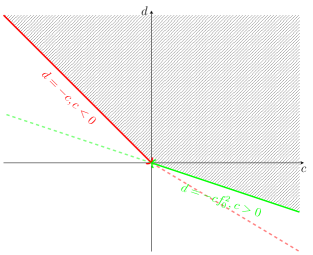
Figure 1. The shaded region together with the red semi-axis represents all $(c,d)\in\mathbb{R}^{2}$ such that $F>0$ on $[f_{0},1)$ for some $f_{0}\in[0,1)$. On the green semi-axis, $F(f_{0})=0$ and $F>0$ on $(f_{0},1)$ so in particular $F\geq 0$.

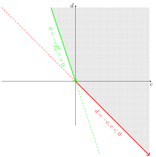
Figure 2. The shaded region together with the red semi-axis represents all $(c,d)\in\mathbb{R}^{2}$ such that $F>0$ on $(1,f_{0}]$ for some $f_{0}\in(1,\infty)$. On the green semi-axis, $F(f_{0})=0$ and $F>0$ on $(1,f_{0})$ so in particular $F\geq 0$.

Proof of Theorem 1.5.

First of all, by Remark 2.6 and Lemma 2.13, we know that $m\neq 0$ and $\kappa\neq 0$, with $m,\kappa>0$ if $f_{0}\in[0,1)$ and $m,\kappa<0$ if $f_{0}\in(1,\infty)$. Next, note that the right-hand side of (LABEL:mainformulap) is continuous on $M$, and non-negative on $M$ if $c,d\in\mathbb{R}$ satisfy $c+d\geq 0$, $cf_{0}^{2}+d\geq 0$ as this gives $F(f)\geq 0$ by Remark 4.1. Now set

$$\mathcal{D}\mathrel{\raise 0.40903pt\hbox{\rm:}\mkern-5.2mu=}\operatorname{div}\left(\frac{F(f)}{f}\|\nabla f\|^{p-3}\,\nabla\|\nabla f\|^{2}+G(f)\|\nabla f\|^{p-1}\,\nabla f\right)$$

on $M$. Then by Theorem 1.4 and its proof, $\mathcal{D}$ is continuous, non-negative, and satisfies (LABEL:mainformulap) on $M$. Aiming for an application of the divergence theorem to $\mathcal{D}$, let us show that $\mathcal{D}$ is integrable on $M$. If $f_{0}>0$, $\mathcal{D}$ is continuous up to $\partial M$; if $f_{0}=0$, we appeal to (2.17) to see that

$$\frac{F(f)}{f}\,\nabla\|\nabla f\|^{2} =2F(f)\operatorname{Ric}(\nabla f,\cdot)$$

so that $\mathcal{D}$ is continuous up to $\partial M$ also when $f_{0}=0$. To analyze the behavior of $\mathcal{D}$ towards the asymptotic end of $(M,g,f)$, let $x\colon M\setminus K\longrightarrow\mathbb{R}^{n}\setminus\overline{B}$ denote a diffeomorphism making $(M,g,f)$ asymptotically flat. The asymptotic assumption (2.6) implies that

$$F(f) =F(f_{m})+o(|x|^{(n-1)(p-1)-(n-2)}),$$

$$F^{\prime}(f) =F^{\prime}(f_{m})+o(|x|^{(n-1)(p-1)}),$$

$$G(f) =G(f_{m})+o(|x|^{(n-1)(p-1)}),$$

$$G^{\prime}(f) =G^{\prime}(f_{m})+o(|x|^{(n-1)(p-1)+2(n-2)})$$

as $|x|\to\infty$, which can be verified most easily via the ODEs for $F$ and $G$ printed in the proof of Theorem 1.4. To study the asymptotics of the first term in $\mathcal{D}$, we apply Bochner’s formula and the static vacuum equation (2.2) to see that

$$\frac{1}{2}\Delta\|\nabla f\|^{2} =\|\nabla^{2}f\|^{2}+\operatorname{Ric}(\nabla f,\nabla f)$$

on $M$, as otherwise we would have to deal with the asymptotic behavior of third derivatives of $f$ about which we have not made any assumptions. Doing so, we find that

$$\operatorname{div}\left(\frac{F(f)}{f}\|\nabla f\|^{p-3}\,\nabla\|\nabla f\|^{2}\right)$$

$$=\left(\frac{F^{\prime}(f)}{f}-\frac{F(f)}{f^{2}}\right)\|\nabla f\|^{p-3}\,\langle\nabla f,\nabla\|\nabla f\|^{2}\rangle+\frac{p-3}{2}\frac{F(f)}{f}\|\nabla f\|^{p-5}\|\nabla\|\nabla f\|^{2}\|^{2}$$

$$\quad+\frac{2F(f)}{f}\|\nabla f\|^{p-3}\,\left(\|\nabla^{2}f\|^{2}+\operatorname{Ric}(\nabla f,\nabla f)\right),$$

where we are using Lemma 2.5 and its consequence that $\operatorname{Crit}f$ is bounded because $m\neq 0$. Taken together with Lemma 2.5, we find

$$\mathcal{D} =\mathcal{D}_{m}+o(|x|^{-n})=o(|x|^{-n})$$

as $|x|\to\infty$. Here, $\mathcal{D}_{m}$ denotes the divergence $\mathcal{D}$ for $f=f_{m}$ and $g=g_{m}$ and we are using that we have seen that $\mathcal{D}_{m}=0$ at the end of Section 3. Hence by (2.11), $\mathcal{D}$ is integrable on $M$ as claimed and we can apply the divergence theorem to it, recalling that $(M,g)$ is geodesically complete up to $\partial M$ by Remark 2.4.

To this end, let $r>0$ be such that $B_{r}\mathrel{\raise 0.40903pt\hbox{\rm:}\mkern-5.2mu=}\left\{x\in\mathbb{R}^{n}\,:\,|x|<r\right\}\supset\overline{B}$ and thus $x^{-1}(\mathbb{R}^{n}\setminus B_{r})\subseteq M$. From the divergence theorem, our choice of unit normal $\nu$ pointing towards infinity, and (2.17), we obtain

$$\int_{M\setminus x^{-1}(\mathbb{R}^{n}\setminus B_{r})}\mathcal{D}\,dV$$

$$\quad=\int_{x^{-1}(\partial B_{r})}\left(\frac{F(f)}{f}\|\nabla f\|^{p-3}\langle\nabla\|\nabla f\|^{2},\nu\rangle+G(f)\|\nabla f\|^{p-1}\langle\nabla f,\,\nu\rangle\right)dS$$

$$\quad\quad-\int_{\partial M}\left(\frac{F(f)}{f}\|\nabla f\|^{p-3}\langle\nabla\|\nabla f\|^{2},\nu\rangle+G(f)\|\nabla f\|^{p-1}\langle\nabla f,\,\nu\rangle\right)dS.$$

Exploiting Lemma 2.5 and the above asymptotics for $F(f)$ and $G(f)$, we find

$$\int_{x^{-1}(\partial B_{r})}\left(\frac{F(f)}{f}\|\nabla f\|^{p-3}\langle\nabla\|\nabla f\|^{2},\nu\rangle+G(f)\|\nabla f\|^{p-1}\langle\nabla f,\,\nu\rangle\right)dS$$

$$=\int_{x^{-1}(\partial B_{r})}\left(\frac{F(f_{m})}{f_{m}}\|\nabla_{m}f_{m}\|_{m}^{p-3}\langle\nabla_{m}\|\nabla_{m}f\|_{m}^{2},\nu_{m}\rangle_{m}+G(f_{m})\|\nabla_{m}f_{m}\|_{m}^{p-1}\langle\nabla_{m}f_{m},\,\nu_{m}\rangle_{m}\right)dS_{\delta}$$

$$\quad+o(1)$$

$$=-\mathcal{F}^{\,c,d}_{\!p}(m)+o(1)$$

as $r\to\infty$, where $\langle\cdot,\cdot\rangle_{m}=g_{m}$ and $\nu_{m}$ denotes the unit normal to $x^{-1}(\partial B_{r})$ with respect to $g_{m}$ pointing to infinity. For the inner boundary integral, we recall from Remark 2.6 that $\nu=\frac{\nabla f}{\|\nabla f\|}$, $\kappa=\|\nabla f\|$ if $f_{0}\in[0,1)$ and $\nu=-\frac{\nabla f}{\|\nabla f\|}$, $\kappa=-\|\nabla f\|$ if $f_{0}\in(1,\infty)$. Exploiting that $f=f_{0}$ and $\kappa$ are constant on $\partial M$ by assumption, we compute

$$\int_{\partial M}\left(\frac{F(f)}{f}\|\nabla f\|^{p-3}\langle\nabla\|\nabla f\|^{2},\nu\rangle+G(f)\|\nabla f\|^{p-1}\langle\nabla f,\,\nu\rangle\right)dS$$

$$=\pm\frac{F_{0}}{f_{0}}|\kappa|^{p-4}\int_{\partial M}\langle\nabla\|\nabla f\|^{2},\nabla f\rangle dS\pm G_{0}|\kappa|^{p}|\partial M|,$$

with $\pm=+$ if $f_{0}\in[0,1)$ and $\pm=-$ if $f_{0}\in(1,\infty)$, respectively. Using (2.3) and (2.1) as well as the Gauss equation, we compute

$$\langle\nabla\|\nabla f\|^{2},\nabla f\rangle=2\nabla^{2}f(\nabla f,\nabla f)=2f_{0}\operatorname{Ric}(\nabla f,\nabla f)$$

$$\quad=2f_{0}\kappa^{2}\operatorname{Ric}(\nu,\nu)=-f_{0}\kappa^{2}\left(\operatorname{R}_{\partial M}-\tfrac{n-2}{n-1}\operatorname{H}^{2}+\|\mathring{h}\|^{2}\right).$$

Combining this with the above, we find

$$\int_{\partial M}\left(\frac{F(f)}{f}\|\nabla f\|^{p-3}\langle\nabla\|\nabla f\|^{2},\nu\rangle+G(f)\|\nabla f\|^{p-1}\langle\nabla f,\,\nu\rangle\right)dS$$

$$=\mp F_{0}|\kappa|^{p-2}\int_{\partial M}\left(\operatorname{R}_{\partial M}-\tfrac{n-2}{n-1}\operatorname{H}^{2}+\|\mathring{h}\|^{2}\right)dS\pm G_{0}|\kappa|^{p}|\partial M|$$

and thus

$$\int_{M}\mathcal{D}\,dV =-\mathcal{F}^{\,c,d}_{\!p}(m)\pm F_{0}|\kappa|^{p-2}\int_{\partial M}\left(\operatorname{R}_{\partial M}-\tfrac{n-2}{n-1}\operatorname{H}^{2}+\|\mathring{h}\|^{2}\right)dS\mp G_{0}|\kappa|^{p}\,|\partial M|.$$

Consequently, for $c,d\in\mathbb{R}$ satisfying $c+d\geq 0$, $cf_{0}^{2}+d\geq 0$, we find (1.14) and (1.15). Equality holds in (1.14) or in (1.15) if and only if equality holds in  (LABEL:mainformulap) and thus $\mathcal{D}=0$ on $M$. Hence if $c+d\geq 0$, $cf_{0}^{2}+d\geq 0$ (but not $c=d=0$), equality in (LABEL:mainformulap) gives $T=0$ and (1.17) as claimed. ∎

Let us now discuss the geometric implications of (1.14) and (1.15) or in other words prove Theorem 1.6 and, in passing, its equivalence to Theorem 1.5.

Proof of Theorem 1.6.

We begin by choosing $f_{0}\in[0,1)$, recalling that $\kappa>0$ and $m>0$ in this case. Choosing the admissible constants $c=1$, $d=-f_{0}^{2}$ in (1.14), we find from Lemma 2.13 that $\kappa=(n-2)\frac{|\mathbb{S}^{n-1}|}{|\partial M|}m$ and thus

$$m\geq\frac{(1-f_{0}^{2})\left(s_{\partial M}\right)^{n-2}}{2}.$$

Choosing instead the admissible constants $c=-1$, $d=1$, (1.14) reduces to

$$(1-f_{0}^{2})|\partial M|\int_{\partial M}\left(\operatorname{R}_{\partial M}-\tfrac{n-2}{n-1}\operatorname{H}^{2}+\|\mathring{h}\|^{2}\right)dS\geq 4(n-1)(n-2)|\mathbb{S}^{n-1}|^{2}\,m^{2}.$$

Moreover, the left-hand side inequality in (1.18) is equivalent to the second of the above inequalities via an algebraic re-arrangement. On the other hand, as (1.14) is linear in $c,d$ and the constraints $c+d\geq 0$, $cf_{0}^{2}+d\geq 0$ are linear as well, the combination of the two above inequalities is equivalent to (1.14). This proves Theorem 1.6 for $f_{0}\in(1,\infty)$.

Next, let us consider $f_{0}\in(1,\infty)$, recalling that $\kappa,m<0$ in this case. Choosing the admissible constants $c=-1$, $d=f_{0}^{2}$ in (1.15), we again find from Lemma 2.13 that $\kappa=(n-2)\frac{|\mathbb{S}^{n-1}|}{|\partial M|}m$ and thus

$$m\leq\frac{(1-f_{0}^{2})\left(s_{\partial M}\right)^{n-2}}{2}.$$

Choosing instead the admissible constants $c=1$, $d=-1$, (1.14) reduces to

$$(f_{0}^{2}-1)|\partial M|\int_{\partial M}\left(\operatorname{R}_{\partial M}-\tfrac{n-2}{n-1}\operatorname{H}^{2}+\|\mathring{h}\|^{2}\right)dS\leq-4(n-1)(n-2)|\mathbb{S}^{n-1}|^{2}\,m^{2}.$$

Moreover, the left-hand side inequality in (1.19) is equivalent to the second of the above inequalities via an algebraic re-arrangement. Again, as (1.15) is linear in $c,d$ and the constraints $c+d\geq 0$, $cf_{0}^{2}+d\geq 0$ are linear as well, the combination of the two above inequalities is equivalent to (1.15). This proves Theorem 1.6 for $f_{0}\in[0,1)$. ∎

We now proceed to proving Theorem 1.1 and Theorem 1.2, where we will use Theorem 1.7 the proof of which will be given in Section 5.

Proof of Theorem 1.1.

To prove Theorem 1.1, we consider the implications of Theorem 1.6 in the setting of Theorem 1.1, i.e., if $f_{0}=0$ and $\partial M$ is a connected static horizon. Then we know that $\operatorname{H}=0$, $\mathring{h}=0$ on $\partial M$ by Remark 2.8 and hence (1.18) reduces to (1.2). Moreover, (1.18) implies (1.3) upon dropping the middle term and squaring. If, in addition, the assumption (1.4) holds then we have equality in (1.3) and thus in both inequalities in (1.18). By Theorem 1.6, this implies that $T=0$ and (1.17) hold on $M$. Applying Theorem 1.7, this proves Theorem 1.1. ∎

Proof of Theorem 1.2.

To see that Theorem 1.2 holds, we consider the implications of Theorem 1.6 in the setting of Theorem 1.2, i.e., if $f_{0}\in(0,1)\cup(1,\infty)$ and $\partial M$ is a connected time slice of a photon surface and thus in particular has constant scalar curvature $\operatorname{R}_{\partial M}$, constant mean curvature $\operatorname{H}$, is totally umbilic ($\mathring{h}=0$) and obeys the photon surface constraint (2.19). When $f_{0}\in(0,1)$, (1.18) gives (1.5). Moreover, dropping the middle term in (1.18) and squaring it gives (1.6). Rewriting (1.6) via the photon surface constraint (2.19) gives

$$\frac{2\kappa\operatorname{H}}{f_{0}} \geq\frac{(n-1)(n-2)(1-f_{0}^{2})}{\left(s_{\partial M}\right)^{2}}.$$

Assuming in addition (1.9) and rewriting it via the photon surface constraint (2.19) gives

$$\frac{2\kappa\operatorname{H}}{f_{0}}+\frac{n-2}{n-1}\operatorname{H}^{2} \leq\frac{(n-1)(n-2)}{\left(s_{\partial M}\right)^{2}}.$$

Taken together, this gives

$$\frac{2\kappa\operatorname{H}}{f_{0}}+\frac{n-2}{n-1}\operatorname{H}^{2} \leq\frac{(n-1)(n-2)}{\left(s_{\partial M}\right)^{2}}\leq\frac{2\kappa\operatorname{H}f_{0}}{1-f_{0}^{2}}$$

Recalling that $\operatorname{H}>0$ from the above or by Proposition 2.11 implies

$$1-f_{0}^{2} \leq\frac{2(n-1)\kappa f_{0}}{(n-2)\operatorname{H}}.$$

On the other hand, the squared left-hand side inequality in (1.5) together with the Smarr formula (2.20) leads to

$$1-f_{0}^{2} \geq\frac{2(n-1)\kappa f_{0}}{(n-2)\operatorname{H}}.$$

Thus, equality holds in all the above inequalities and hence in (1.5), too. By Theorem 1.6, this implies that $T=0$ and (1.17) hold on $M$. By Theorem 1.7, this proves Theorem 1.2 when $f_{0}\in(0,1)$. For $f_{0}\in(1,\infty)$, the argument is the same with reversed signs. ∎

5. Recovering the Schwarzschild geometry

In Section 4, we have proven Theorems 1.1 and 1.2 relying on Theorem 1.7 which we have not yet proved. Proving Theorem 1.7 will be the goal of this section. To this end, we will use the following straightforward remark.

Remark 5.1 (Regular foliation).

Let $(M^{n},g,f)$ be a static system with $f\neq 1$. Then (1.17) is equivalent to

(5.1) $$\nabla\left[\frac{\|\nabla f\|^{2}}{(1-f^{2})^{\frac{2(n-1)}{n-2}}}\right] =0$$

on $M$. In particular, provided that $f\neq 1$, (1.17) asserts that either $\nabla f=0$ on $M$ or $f$ regularly foliates $M$, i.e., $\nabla f\neq 0$ on $M$.

Proof of Theorem 1.7.

By Remark 5.1, we know that $f$ regularly foliates $M$ because $\nabla f=0$ on $M$ contradicts Remark 2.6. Moreover, we know that $\|\nabla f\|$ is constant on each level set $\Sigma_{f}^{n-1}$ of $f$, more precisely

(5.2) $$\|\nabla f\| =|\kappa|\left(\frac{1-f^{2}}{1-f_{0}^{2}}\right)^{\frac{n-1}{n-2}}$$

holds on $M$, where $\kappa\mathrel{\raise 0.40903pt\hbox{\rm:}\mkern-5.2mu=}\nu(f)|_{\partial M}$ is also necessarily constant; note that $|\kappa|>0$ by Remark 2.6. From (2.27) and the static vacuum equations (2.1), (2.2), we find that the level sets of $f$ are totally umbilic: Indeed, the second fundamental form $h_{f}$ and the mean curvature $\operatorname{H}_{f}$ of any level set $\Sigma_{f}$ of $f$ are given by

$$h_{f} =\left.\frac{\nabla^{2}f}{\|\nabla f\|}\right|_{T\Sigma_{f}\times T\Sigma_{f}}=\left.\frac{f\operatorname{Ric}}{\|\nabla f\|}\right|_{T\Sigma_{f}\times T\Sigma_{f}}=-\frac{f\operatorname{Ric}(\nabla f,\nabla f)}{(n-1)\|\nabla f\|^{3}}g_{f},$$

(5.3) $$\operatorname{H}_{f} =-\frac{f\operatorname{Ric}(\nabla f,\nabla f)}{\|\nabla f\|^{3}}=-\frac{\nabla^{2}f(\nabla f,\nabla f)}{\|\nabla f\|^{3}},$$

respectively, where $g_{f}$ denotes the induced metric on $\Sigma_{f}$. Now, we use that $f$ regularly foliates $M$ to construct local coordinates $(f,\varphi^{J})_{J=1}^{n-1}$ by flowing local coordinates $(\varphi^{J})_{J=1}^{n-1}$ of $\partial M$ along $\frac{\nabla f}{\|\nabla f\|^{2}}$. Note that such coordinate patches cover $M$ as $M$ is geodesically complete up to $\partial M$ by Remark 2.4. In these coordinates, one finds $\partial_{f}=\frac{\nabla f}{\|\nabla f\|^{2}}$ and

$$g =\frac{1}{\|\nabla f\|^{2}}df^{2}+g_{f},$$

$$\operatorname{H}_{f} =-\partial_{f}\|\nabla f\|,$$

$$h_{f} =\frac{\|\nabla f\|}{2}\partial_{f}g_{f}$$

on $\Sigma_{f}$ as is well-known for the level set flow of a harmonic function. For the sake of completeness, let us mention that the second to last identity follows from (5.3) via (2.17) and the last identity follows from a direct computation of $h_{f}$ using the special form of the Christoffel symbols derived from the special form of the metric $g$ in the coordinates $(f,\varphi^{J})_{J=1}^{n-1}$. In particular, $\operatorname{H}_{f}$ is constant on $\Sigma_{f}$. Combining the last two of the above identities with the umbilicity of $\Sigma_{f}$ and (5.2), one gets

$$\partial_{f}g_{f} =\frac{4f}{(n-2)(1-f^{2})}g_{f}.$$

Let $g_{\partial M}$ denote the induced metric on $\partial M$. By standard ODE theory, the unique solution to this equation with initial value $g_{f_{0}}=g_{\partial M}$ is given by

$$g_{f} =\left(\frac{1-f_{0}^{2}}{1-f^{2}}\right)^{\frac{2}{n-2}}g_{\partial M}.$$

Together with (5.2), defining the surface area radius $s(f)\mathrel{\raise 0.40903pt\hbox{\rm:}\mkern-5.2mu=}\left(\frac{1-f_{0}^{2}}{1-f^{2}}\right)^{\frac{1}{n-2}}s_{\partial M}$ of $\Sigma_{f}$ on the range of $f$ with $s_{\partial M}$ the surface area radius of $\partial M$ as defined in (1.1), this gives

(5.4) $$f(s) =\sqrt{1-\left(\frac{s_{\partial M}}{s}\right)^{n-2}(1-f_{0}^{2})}\mathrel{=\mkern-5.2mu\raise 0.40903pt\hbox{\rm:}}\sqrt{1-\frac{2\mu}{s^{n-2}}}$$

for $s\in[s_{\partial M},\infty)$ with $\mu>0$ when $f_{0}\in[0,1)$ and $\mu<0$ when $f_{0}\in(1,\infty)$. Moreover, we find

$$g =\frac{1}{\kappa^{2}}\left(\frac{1-f_{0}^{2}}{1-f^{2}}\right)^{\frac{2(n-1)}{n-2}}df^{2}+\left(\frac{1-f_{0}^{2}}{1-f^{2}}\right)^{\frac{2}{n-2}}g_{\partial M}$$

$$=\left(\frac{(n-2)\mu}{\kappa(s_{\partial M})^{n-1}}\right)^{2}\frac{ds^{2}}{f(s)^{2}}+\left(\frac{s}{s_{\partial M}}\right)^{2}g_{\partial M}$$

on $[s_{\partial M},\infty)\times\partial M$ except when $f_{0}=0$ where this formula only holds on $(s_{\partial M},\infty)\times\partial M$. Using the Smarr formula (2.13) and the definition of $\mu$ in (5.4), we find

(5.5) $$g =\frac{\mu^{2}}{m^{2}}\frac{ds^{2}}{f(s)^{2}}+\left(\frac{s}{s_{\partial M}}\right)^{2}g_{\partial M}$$

on $[s_{\partial M},\infty)\times\partial M$ (respectively on $(s_{\partial M},\infty)\times\partial M$ when $f_{0}=0$). To see that $(\partial M,g_{\partial M})$ is indeed isometric to the standard round $(n-1)$-sphere of radius $s_{\partial M}$, we need to carefully consider the asymptotic decay of $g$. To this end, let $x\colon M\setminus K\longrightarrow\mathbb{R}^{n}\setminus\overline{B}$ denote a diffeomorphism making $(M,g,f)$ asymptotically flat and denote the induced coordinates by $(x^{i})$. For convenience, let us switch to standard polar coordinates $(r,\theta^{J})_{J=1}^{n-1}$ for $\mathbb{R}^{n}$ associated to $(x^{i})$ so that $(\partial_{\theta^{K}})^{i}=O(r)$ as $r=|x|\to\infty$ and $\delta(\partial_{\theta^{I}},\partial_{\theta^{J}})=r^{2}(g_{\mathbb{S}^{n-1}})(\partial_{\theta^{I}},\partial_{\theta^{J}})$ for $I,J,K=1,\dots,n-1$. Then by (2.6), we find

$$1-\frac{2\mu}{s^{n-2}} =f(s)^{2}=1-\frac{2m}{r^{n-2}}+o_{2}(r^{-(n-2)})$$

as $r=|x|\to\infty$ which implies $s=\frac{\mu}{m}r+o_{2}(r)$ as $r\to\infty$. Moreover, taking a $\partial_{\theta^{K}}$-derivative of this identity, one sees that

$$\frac{\partial s}{\partial\theta^{K}} =\partial_{\theta^{I}}o_{2}(r)=(\partial_{\theta^{K}})^{i}o_{1}(1)=o_{1}(r)$$

as $r\to\infty$ for $K=1,\dots,n-1$. As implicitly done above and as usual, we will interpret $g_{\partial M}$ as an $s$-independent tensor field on $M$ which is applied to tensor fields on $M$ by first projecting them tangentially to the level sets $\Sigma_{f}\approx\{s(f)\}\times\partial M$ of $f$. Similarly, we interpret $g_{\mathbb{S}^{n-1}}$ as an $r$-independent tensor field on $\mathbb{R}^{+}\times\mathbb{S}^{n-1}$ by projection onto round spheres as usual. Exploiting this convention, our asymptotic flatness assumptions in Definition 2.2 combined with (5.5) give

$$1+o_{2}(1)=g_{rr} =\frac{\mu^{4}}{m^{4}}+o_{1}(1)+\frac{\mu^{2}}{m^{2}}\frac{r^{2}}{(s_{\partial M})^{2}}(1+o_{1}(1))(g_{\partial M})_{rr},$$

$$o_{2}(r^{1})=g_{r\theta^{K}} =o_{1}(r)+\frac{\mu^{2}}{m^{2}}\frac{r^{2}}{(s_{\partial M})^{2}}(1+o_{1}(1))(g_{\partial M})_{r\theta^{K}},$$

$$r^{2}(g_{\mathbb{S}^{n-1}})_{\theta^{I}\theta^{J}}+o_{2}(r^{2x})=g_{\theta^{I}\theta^{J}} =o_{1}(r^{2})+\frac{\mu^{2}}{m^{2}}\frac{r^{2}}{(s_{\partial M})^{2}}(1+o_{1}(1))(g_{\partial M})_{\theta^{I}\theta^{J}}$$

as $r\to\infty$ for $I,J,K=1,\dots,n-1$. This can easily be rewritten as

$$(g_{\partial M})_{ij} =\frac{m^{2}}{\mu^{2}}(s_{\partial M})^{2}\,(g_{\mathbb{S}^{n-1}})_{ij}+o_{1}(1)$$

as $r\to\infty$ for $i=1,\dots,n$. As $g_{\partial M}$ is independent of $s$, this naturally informs us that

$$(g_{\partial M})_{\varphi^{I}\varphi^{J}} =\frac{m^{2}}{\mu^{2}}(s_{\partial M})^{2}\,(g_{\mathbb{S}^{n-1}})_{\varphi^{I}\varphi^{J}}$$

for $I,J=1,\dots,n-1$ with respect to the local coordinates $(\varphi^{J})$ on $\partial M$. To see this, one proceeds as above to see that $r=\frac{m}{\mu}s+o_{2}(s)$ as $s\to\infty$ so that $\frac{\partial r}{\partial\varphi^{K}}=o_{1}(s)$ as $s\to\infty$ for $K=1,\dots,n-1$. This allows us to conclude $(\partial M,g_{\partial M})$ is isometric to the round $(n-1)$-sphere of radius $\frac{m}{\mu}s_{\partial M}$ upon recalling that $\frac{m}{\mu}>0$. From the definition of $s_{\partial M}$, we conclude that $\mu=m$. Thus, by (5.5) and Remark 2.4, we deduce that $(M,g)$ must be isometric to the piece $[s_{\partial M},\infty)\times\mathbb{S}^{n-1}$ of the Schwarzschild manifold $(M^{n}_{m},g_{m})$ of mass $m$, with $f$ corresponding to $f_{m}$ respectively that $(M\setminus\partial M,g)$ must be isometric to the piece $(s_{\partial M},\infty)\times\mathbb{S}^{n-1}$ of the Schwarzschild manifold $(M^{n}_{m},g_{m})$ of mass $m$ when $f_{0}=0$, with $f$ corresponding to $f_{m}$. Switching to isotropic coordinates then also allows us to conclude that the claims extend to $\partial M$ when $f_{0}=0$. ∎

6. Discussion and monotone functionals

In Theorem 1.4 and its proof, we have seen that the divergence of the vector field

(6.1) $$Z\mathrel{\raise 0.40903pt\hbox{\rm:}\mkern-5.2mu=}\frac{F(f)}{f}\|\nabla f\|^{p-3}\,\nabla\|\nabla f\|^{2}+G(f)\|\nabla f\|^{p-1}\,\nabla f$$

is continuous and non-negative for all $n\geq 3$, $p\geq 3$, $c,d\in\mathbb{R}$ with $c+d\geq 0$, $cf_{0}^{2}+d\geq 0$, and $F$ and $G$ as defined in (1.11), (1.12). We exploited this to prove the parametric geometric inequalities in Theorem 1.5 and, equivalently, the geometric inequalities in Theorem 1.6, by applying the divergence theorem to $Z$ on $M$ and evaluating the corresponding surface integrals at $\partial M$ with $f=f_{0}$ on $\partial M$, $f_{0}\in[0,1)\cup(1,\infty)$, and at infinity. Of course, one can also apply to divergence theorem to $Z$ on suitable open submanifolds $N$ of $M$ and exploit the non-negativity of $\operatorname{div}Z$ to obtain estimates between the different components of $\partial N$. In view of the fact that we are using an approach based on potential theory, and in order to compare our technique of proof to the monotone functional approach by Agostiniani and Mazzieri [1], it will be most interesting to study such $N$ for which $\partial N$ consists of level sets of the lapse function $f$.

Let us focus on the case $f_{0}\in[0,1)$ which coincides with the situation studied in [1], noting that the case $f_{0}\in(1,\infty)$ can be treated the same way. Given a static vacuum system $(M^{n},g,f)$, $n\geq 3$, with boundary $\partial M$ such that $f=f_{0}$ on $\partial M$ for some $f_{0}\in[0,1)$, and given $p\geq 3$, $c,d\in\mathbb{R}$ and $F$ and $G$ as defined in (1.11), (1.12), we define the functionals $\mathcal{H}_{p}^{c,d}\colon[f_{0},1)\to\mathbb{R}$ by

(6.2) $$\mathcal{H}_{p}^{c,d}(f) \mathrel{\raise 0.40903pt\hbox{\rm:}\mkern-5.2mu=}\int_{\Sigma_{f}}\langle Z,\nu\rangle\,dS=\int_{\Sigma_{f}}\left[\frac{F(f)}{f}\|\nabla f\|^{p-4}\langle\nabla\|\nabla f\|^{2},\nabla f\rangle+G(f)\|\nabla f\|^{p}\right]dS,$$

where $\Sigma_{f}$ denotes the $f$-level set of the lapse function $f$. $\mathcal{H}_{p}^{c,d}(f)$ is clearly well-defined on every regular level set of $f$, including $\Sigma_{f=0}$ if $f_{0}=0$ as we have seen in the proof of Theorem 1.5. As $f$ is harmonic and proper, we know that $\Sigma_{f}$ is compact. By the work of Hardt–Simon [19] and Lin [26], we know that the $n-1$-dimensional Hausdorff measure of $\Sigma_{f}$ is finite, $\mathcal{H}^{n-1}(\Sigma_{f})<\infty$. Moreover, by the work of Cheeger–Naber–Valtorta [15] and Hardt–Hoffmann-Ostenhof–Hoffmann-Ostenhof–Nadirashvili [18], we know that the Hausdorff dimension of the critical set $\operatorname{Crit}f$ is bounded above by $n-2$. Taken together, this shows that the normal vector field $\nu$ is defined $\mathcal{H}^{n-1}$-almost everywhere on $\Sigma_{f}$. It is also essentially bounded and $Z$ is continuous on $M$. Moreover, the hypersurface area element $dS$ has a density with respect to the Hausdorff element $d\mathcal{H}^{n-1}$ which is well-defined and bounded $\mathcal{H}^{n-1}$-almost everywhere on $\Sigma_{f}$. Taken together, this shows that $\mathcal{H}_{p}^{c,d}(f)$ is well-defined also on level sets $\Sigma_{f}$ containing critical points of $f$. The same arguments show that the mean curvature $\operatorname{H}$ is defined $\mathcal{H}^{n-1}$-almost everywhere on $\Sigma_{f}$ also for level sets $\Sigma_{f}$ containing critical points of $f$. A direct computation as in the proof of Theorem 1.5 then shows that

(6.3) $$\mathcal{H}_{p}^{c,d}(f)=-\frac{2F(f)}{f}\int_{\Sigma_{f}}\|\nabla f\|^{p-1}\left[\operatorname{H}-\frac{fG(f)}{2F(f)}\|\nabla f\|^{p}\right]dS$$

holds for all values $f\in[f_{0},1)$. Next, we would like to apply the divergence theorem to $Z$ on domains of the form $\{f_{1}<f<f_{b}\}$ for some not necessarily regular values $f_{0}\leq f_{1}<f_{2}<1$ of $f$ to conclude that $\mathcal{H}^{c,d}_{p}$ is monotonically increasing provided that $c+d\geq 0$, $cf_{0}^{2}+d\geq 0$ via Theorem 1.4. Of course, if $f_{1},f_{2}$ are regular, the divergence theorem readily applies as $Z$ and $\operatorname{div}Z$ are continuous on $M$ and $\operatorname{div}Z$ is integrable on $M$. To see that the divergence theorem applies even when one or both of $f_{1},f_{2}$ are singular values of $f$, we would like to apply a slight generalization of the divergence theorem given for example in [1, Theorem A.1]. We have seen in the proof of Theorem 1.4 that $Z$ is differentiable also across $\operatorname{Crit}f$. Moreover, by the asymptotic considerations in the proof of Theorem 1.5, we know that $\|\operatorname{div}Z\|$ is bounded on $M$ because $\operatorname{div}Z=\mathcal{D}=o(|x|^{-n})$ as $|x|\to\infty$ and arguing similarly via Lemma 2.5 one finds that $\|Z\|=O(|x|^{-(n-1)})$ as $|x|\to\infty$ so that $\|Z\|$ is also bounded on $M$. Choosing the domain $E=\{f_{1}<f<f_{2}\}$ in [1, Theorem A.1], we clearly have that $E$ is bounded as $f\to 1$ as $|x|\to\infty$ by our asymptotic assumptions. For the same reason, $\partial E$ is compact. As discussed above, we know that $\mathcal{H}^{n-1}(\partial E)<\infty$. Setting $\Gamma\mathrel{\raise 0.40903pt\hbox{\rm:}\mkern-5.2mu=}E\setminus\operatorname{Crit}f$ and $\Sigma\mathrel{\raise 0.40903pt\hbox{\rm:}\mkern-5.2mu=}E\cap\operatorname{Crit}f$, we have $\partial E=\Gamma\sqcup\Sigma$ such that $\Gamma$ is a smooth regular hypersurface by the inverse function theorem. In order to apply [1, Theorem A.1], it hence only remains to verify that $B_{\varepsilon}(\Sigma)\mathrel{\raise 0.40903pt\hbox{\rm:}\mkern-5.2mu=}\bigcup_{x\in\Sigma}B_{\varepsilon}(x)$ satisfies $\mathcal{H}^{n}(B_{\varepsilon}(\Sigma))=o(\varepsilon)$ as $\varepsilon\to 0+$. To see this, we follow [1, proof of Proposition 4.1] and apply [15, Theorem 1.17] to conclude that for every $\eta>0$ there exists a constant $C_{\eta}>0$ such that $\mathcal{H}^{n}(B_{\varepsilon}(\Sigma))\leq C_{\eta}\,\varepsilon^{2-\eta}$ as $\varepsilon\to 0+$ because $f$ is harmonic. Choosing any $\eta>1$ then shows the desired decay and thus permits us to apply the divergence theorem [1, Theorem A.1] to $Z$ on $\{f_{1}<f<f_{2}\}$, obtaining

(6.4) $$\int_{\{f_{1}<f<f_{2}\}}\operatorname{div}Z\,dV=\int_{\Gamma}\langle Z,\nu\rangle\,dS,$$

where $dV$ denotes the volume element of $(M,g)$. As $\Sigma$ has Hausdorff dimension bounded above by $n-2$, $Z$ extends continuously to $\partial E$ and $\nu$ is well-defined and essentially bounded almost everywhere on $\partial E$, the domain of integration on the right-hand side in (6.4) can be replaced by $\partial E$, leading to the desired divergence theorem on $\{f_{1}<f<f_{2}\}$. This allows us to conclude that $\mathcal{H}_{p}^{c,d}$ is monotonically increasing provided that $c+d\geq 0$, $cf_{0}^{2}+d\geq 0$. Moreover, by Theorem 1.5 and its proof, we know that

(6.5) $$\lim_{f\to 1-}\mathcal{H}_{p}^{c,d}(f)=-\mathcal{F}_{p}^{c,d}$$

with $\mathcal{F}_{p}^{c,d}$ as in (1.16), recalling that $f$ has no critical values near infinity. Moreover, recall from the end of Section 3 that $\mathcal{H}_{p}^{c,d}=-\mathcal{F}_{p}^{c,d}$ on $[0,1)$ for the Schwarzschild system $(M^{n}_{m},g_{m},f_{m})$ of mass $m>0$. From Theorems 1.4 and 1.5, we know that (suitable subsets of) the Schwarzschild system are the only static vacuum systems satisfying this identity.

Let us now relate the functional $\mathcal{H}_{p}^{c,d}$ from (6.2) to the functional $U_{p}$ and its derivative introduced in [1]. In our notation, these functionals are given by

(6.6) $$U_{p}(f) \mathrel{\raise 0.40903pt\hbox{\rm:}\mkern-5.2mu=}\left(\frac{2m}{1-f^{2}}\right)^{\frac{(p-1)(n-1)}{n-2}}\int_{\Sigma_{f}}\|\nabla f\|^{p}\,dS,$$

(6.7) $$U_{p}^{\prime}(f) =-(p-1)\left(\frac{2m}{1-f^{2}}\right)^{\frac{(p-1)(n-1)}{n-2}}\int_{\Sigma_{f}}\|\nabla f\|^{p-1}\left[\operatorname{H}-\frac{2(n-1)f\|\nabla f\|}{(n-2)(1-f^{2})}\right]dS.$$

From this, one readily computes that

(6.8) $$U_{p}(f) =\frac{\mu_{p}}{4(1-f_{0}^{2})}\left[\frac{f^{2}-f_{0}^{2}}{1-f^{2}}\mathcal{H}_{p}^{-1,1}(f)-\mathcal{H}_{p}^{1,-f_{o}^{2}}(f)\right],$$

(6.9) $$U_{p}^{\prime}(f) =\frac{\mu_{p}f}{2(1-f^{2})^{2}}\mathcal{H}_{p}^{-1,1}(f)$$

for $\mu_{p}\mathrel{\raise 0.40903pt\hbox{\rm:}\mkern-5.2mu=}(p-1)(2m)^{\frac{(p-1)(n-1)}{n-2}}>0$. In particular, $U_{p}^{\prime}$ is monotonically increasing with $\mathcal{H}_{p}^{-1,1}$ because $\frac{\mu_{p}f}{2(1-f^{2})^{2}}$ is strictly monotonically increasing. This shows that $U_{p}$ is actually convex, a result we could not find in [1]. Note that $U_{p}$ and $U_{p}^{\prime}$ are computed from $\mathcal{H}_{p}^{c,d}$ using only the ”extremal” values of $(c,d)$ (normalized to $|c|=1$) as in the proofs of Theorems 1.1 and 1.2. Conversely, one obtains

(6.10) $$\mu_{p}\mathcal{H}_{p}^{c,d}(f) =\frac{2(cf^{2}+d)(1-f^{2})}{f}U_{p}^{\prime}(f)-4(c+d)U_{p}(f)$$

In particular, by [1, Theorem 1.1], $\mathcal{H}_{p}^{c,d}$ is continuous at $f=0$ and

(6.11) $$\mathcal{H}_{p}^{c,d}(0) =2dU_{p}^{\prime\prime}(0)-4(c+d)U_{p}(0),$$

with $U_{p}^{\prime\prime}(0)\mathrel{\raise 0.40903pt\hbox{\rm:}\mkern-5.2mu=}\lim_{f\searrow 0}\frac{U_{p}^{\prime}(f)}{f}$ as in [1].

This comparison of the monotone functionals $\mathcal{H}^{c,d}_{p}$ and $U_{p}$ shows that our divergence theorem approach leads to very similar results as the monotone functional approach by Agostiniani and Mazzieri [1], in some sense lifting the monotonicity from a derivative to the functional itself. This allows for weaker decay assumptions and circumvents the conformal change to an asymptotically cylindrical picture as introduced in [1]. In particular, working directly with the divergence theorem in the static system makes the analysis of the equality case much simpler, avoiding the need to appeal to a splitting theorem.

Consequently, our approach gives new proofs for all geometric inequalities for black hole horizons described in [1, Section 2.2] and the Willmore-type inequalities for black hole horizons and other level sets of the lapse function $f$ described in [1, Section 2.3]. In particular, we would like to point out that the right-hand side inequality in (1.3) is the Riemannian Penrose inequality. We hence in particular reprove the Riemannian Penrose inequality for asymptotically flat static vacuum systems with connected black hole inner boundary (but with the extra assumption (1.4) necessary to conclude rigidity).

We also extend the results from [1] to the negative mass case, i.e., to $f_{0}\in(1,\infty)$.

References

- [1] Virginia Agostiniani and Lorenzo Mazzieri, On the geometry of the level sets of bounded static potentials, Communications in Mathematical Physics 355 (2017), no. 1, 261–301.
- [2] Simon Brendle, Uniqueness of gradient Ricci solitons, Mathematical Research Letters 18 (2011), no. 03, 531–538.
- [3] Gary L. Bunting and Abdul K. M. Masood-ul Alam, Nonexistence of multiple black holes in asymptotically Euclidean static vacuum space-time, General Relativity and Gravitation 19 (1987), no. 2, 147–154.
- [4] Huai-Dong Cao and Qiang Chen, On Locally Conformally Flat Gradient Steady Ricci Solitons, Transactions of the American Mathematical Society 364 (2012), no. 5, 2377–2391.
- [5] Huai-Dong Cao and Qiang Chen, On Bach-flat gradient shrinking Ricci solitons, Duke Mathematical Journal 162 (2013), no. 6, 1149–1169.
- [6] Carla Cederbaum, Rigidity properties of the Schwarzschild manifold in all dimensions, in preparation.
- [7] Carla Cederbaum, The Newtonian Limit of Geometrostatics, Ph.D. thesis, FU Berlin, 2012, arXiv:1201.5433v1.
- [8] by same author, Uniqueness of photon spheres in static vacuum asymptotically flat spacetimes, Complex Analysis and Dynamical Systems VI, Contemporary Mathematics, American Mathematical Society, Providence, RI, 2014.
- [9] Carla Cederbaum, A geometric boundary value problem related to the static equations in General Relativity, Analysis, Geometry and Topology of Positive Scalar Curvature Metrics, Oberwolfach report, no. 36/2017, EMS Press, 2017.
- [10] Carla Cederbaum, Albachiara Cogo, and Axel Fehrenbach, Uniqueness of equipotential photon surfaces in static vacuum asymptotically flat spacetimes: three different approaches, in preparation.
- [11] Carla Cederbaum and Gregory J. Galloway, Uniqueness of photon spheres via positive mass rigidity, Communications in Analysis and Geometry 25 (2017), no. 2, 303–320.
- [12] by same author, Photon surfaces with equipotential time slices, Journal of Mathematical Physics 62 (2021), no. 3, Paper No. 032504, 22. MR 4236797
- [13] Carla Cederbaum, Melanie Graf, and Jan Metzger, Initial data sets that do not satisfy the Regge–Teitelboim conditions, in preparation.
- [14] Carla Cederbaum, Sophia Jahns, and Olivia Vičánek Martínez, On equipotential photon surfaces in (electro-)static spacetimes of arbitrary dimension, arxiv:2311.17509https://arxiv.org/abs/2311.17509.
- [15] Jeff Cheeger, Aaron Naber, and Daniele Valtorta, Critical sets of elliptic equations, Communications on Pure and Applied Mathematics 68 (2015), no. 2, 173–209.
- [16] Clarissa-Marie Claudel, Kumar Shwetketu Virbhadra, and George F. R. Ellis, The Geometry of Photon Surfaces, J. Math. Phys. 42 (2001), no. 2, 818–839.
- [17] Gary W. Gibbons, Daisuke Ida, and Tetsuya Shiromizu, Uniqueness and Non-Uniqueness of Static Vacuum Black Holes in Higher Dimensions, Progress of Theoretical Physics Supplement 148 (2002), 284–290.
- [18] Robert M. Hardt, Maria Hoffmann-Ostenhof, Thomas Hoffmann-Ostenhof, and Nikolai S. Nadirashvili, Critical sets of solutions to elliptic equations, Journal of Differential Geometry 51 (1999), no. 2, 359–373.
- [19] Robert M. Hardt and Leon Simon, Nodal sets for solutions of elliptic equations, Journal of Differential Geometry 30 (1989), no. 2, 505–522.
- [20] Markus Heusler, Black Hole Uniqueness Theorems, Cambridge Lecture Notes in Physics, Cambridge University Press, Cambridge, 1996.
- [21] Stefan Hollands and Akihiro Ishibashi, Black hole uniqueness theorems in higher dimensional spacetimes, Classical and Quantum Gravity 29 (2012), 163001.
- [22] Seungsu Hwang, A Rigidity Theorem for Ricci Flat Metrics, Geometriae Dedicata 71 (1998), no. 1, 5–17.
- [23] Werner Israel, Event Horizons in Static Vacuum Space-Times, Physical Review 164 (1967), no. 5, 1776–1779.
- [24] Daniel Kennefick and Niall Ó Murchadha, Weakly decaying asymptotically flat static and stationary solutions to the Einstein equations, Class. Quantum Grav. 12 (1995), no. 1, 149.
- [25] Benedito Leandro and Newton Solórzano, Static perfect fluid spacetime with half conformally flat spatial factor, manuscripta mathematica 160 (2019), 51–63.
- [26] F.-H. Lin, Nodal sets of solutions of elliptic and parabolic equations, Communications on Pure and Applied Mathematics 44 (1991), no. 3, 287–308.
- [27] Joachim Lohkamp, The Higher Dimensional Positive Mass Theorem I, 2016, arXiv:math/0608795v2.
- [28] Pengzi Miao, A remark on boundary effects in static vacuum initial data sets, Classical and Quantum Gravity 22 (2005), no. 11, L53–L59.
- [29] Henning Müller zum Hagen, David C. Robinson, and Hans Jürgen Seifert, Black holes in static vacuum space-times, General Relativity and Gravitation 4 (1973), no. 1, 53–78.
- [30] Volker Perlick, On totally umbilici submanifolds of semi-Riemannian manifolds, Nonlinear Analysis 63 (2005), no. 5-7, e511–e518.
- [31] Simon Raulot, A spinorial proof of the rigidity of the Riemannian Schwarzschild manifold, Classical and Quantum Gravity 38 (2021), no. 8, 085015.
- [32] David C. Robinson, A simple proof of the generalization of Israel’s theorem, General Relativity and Gravitation 8 (1977), no. 8, 695–698.
- [33] David C. Robinson, Four decades of black hole uniqueness theorems, Classical and Quantum Gravity 38 (2012), no. 8, 115–143.
- [34] Richard M. Schoen and Shing-Tung Yau, Complete manifolds with nonnegative scalar curvature and the positive action conjecture in general relativity, Proceedings of the National Academy of Sciences in the U.S.A. 76 (1979), no. 3, 1024–1025.
- [35] by same author, On the Proof of the Positive Mass Conjecture in General Relativity, Communications in Mathematical Physics 65 (1979), no. 1, 45–76.
- [36] Richard M. Schoen and Shing-Tung Yau, Positive Scalar Curvature and Minimal Hypersurface Singularities, 2017, arxiv:1704.05490.
- [37] Edward Witten, A new proof of the positive energy theorem, Communications in Mathematical Physics 80 (1981), no. 3, 381–402.