Current density functional framework for spin–orbit coupling: Extension to periodic systems

Abstract

Spin–orbit coupling induces a current density in the ground state, which consequently requires a generalization for meta-generalized gradient approximations. That is, the exchange-correlation energy has to be constructed as an explicit functional of the current density and a generalized kinetic energy density has to be formed to satisfy theoretical constraints. Herein, we generalize our previously presented formalism of spin–orbit current density functional theory [Holzer et al., J. Chem. Phys. 157, 204102 (2022)] to non-magnetic and magnetic periodic systems of arbitrary dimension. Besides the ground-state exchange-correlation potential, analytical derivatives such as geometry gradients and stress tensors are implemented. The importance of the current density is assessed for band gaps, lattice constants, magnetic transitions, and Rashba splittings. For the latter, the impact of the current density may be larger than the deviation between different density functional approximations.

I Introduction

In the constantly evolving field of density functional theory (DFT), especially the construction of meta-generalized gradient approximations (meta-GGAs) has received great attention over the last two decades. Burke (2012); Becke (2014); Sun, Ruzsinszky, and Perdew (2015); Mardirossian and Head-Gordon (2017) Modern meta-GGAs use the iso-orbital constraint and the von-Weizäcker inequality to identify one-electron regions and, thus cancelling self-interaction errors in single electron regions. Sun, Ruzsinszky, and Perdew (2015); Tao and Mo (2016) According to benchmark calculations, Mardirossian and Head-Gordon (2017); Hao et al. (2013); Mo et al. (2017); Goerigk et al. (2017); Franzke and Yu (2022a, b); Becke (2022); Borlido et al. (2019); Holzer, Franzke, and Kehry (2021); Holzer and Franzke (2022); Lee et al. (2021); Ghosh et al. (2022); Kovás et al. (2022); Liang et al. (2022); Franzke (2023); Kovács, Blaha, and Madsen (2023); Lebeda et al. (2023) meta-GGAs outperform the preceding generalized gradient approximations (GGAs) at roughly the same computational cost. However, external magnetic fields Furness et al. (2015); Tellgren et al. (2014); Irons, David, and Teale (2021); Pausch and Holzer (2022) or spin–orbit coupling Saue (2005, 2011); Pyykkö (2012) necessitate further generalizations for meta-GGAs to meet theoretical constrains, as the current density alters the curvature of the Fermi hole in its second-order Taylor expansion. Dobson (1993); Tao (2005); Pittalis et al. (2007); Räsänen, Pittalis, and Proetto (2010); Pittalis, Räsänen, and Gross (2009); Bates and Furche (2012); Maier, Ikabata, and Nakai (2020); Holzer, Franzke, and Pausch (2022); Desmarais et al. (2024a, b) Density functional approximations (DFAs) constructed by taking into account this change in curvature are termed “CDFT” functionals. Tellgren et al. (2012); Furness et al. (2015) CDFT based approximations are for example necessary for the iso-orbital indicator to remain bounded between 0 and 1. Holzer, Franzke, and Pausch (2022); Maier, Ikabata, and Nakai (2020) In external magnetic fields, this correction is even necessary to guarantee gauge-invariance. Furness et al. (2015); Pausch and Holzer (2022); Holzer, Franzke, and Pausch (2022)

Furthermore, certain current-carrying ground states also heavily depend on the correct introduction of the current density, with a failure to account for them leading to large deviation for meta-GGAs. Becke (2002); Holzer, Franzke, and Pausch (2022) We recently presented a current-dependent formulation of density functional theory for spin–orbit coupling in the molecular regime. Holzer, Franzke, and Pausch (2022) Here, inclusion of the current density leads to notable changes for both closed-shell Kramers-restricted (KR) and open-shell Kramers-unrestricted (KU) calculations.

To account for the change in Fermi hole curvature, the kinetic energy density $\tau$ is generalized with the current density $\vec{j}$. In a two-component (2c) non-collinear formalism, Kübler et al. (1988); Van Wüllen (2002); Saue and Helgaker (2002); Armbruster et al. (2008); Peralta, Scuseria, and Frisch (2007); Scalmani and Frisch (2012); Bulik et al. (2013); Baldes and Weigend (2013); Egidi et al. (2017); Komorovsky, Cherry, and Repisky (2019); Desmarais et al. (2021) this results in the generalized current density

$$\tilde{\tau}_{\uparrow,\downarrow}=\tau_{\uparrow,\downarrow}-\frac{|\vec{j}_{\uparrow,\downarrow}|^{\,2}}{2n_{\uparrow,\downarrow}}$$ (1)

based on the spin-up and down quantities. Holzer, Franzke, and Pausch (2022) These are formed with the particle and spin-magnetization contributions, e.g. the spin-up and down electron density $n_{\uparrow,\downarrow}$ follows as

$$n_{\uparrow,\downarrow}(\vec{r})=\frac{1}{2}\left[n(\vec{r})\pm|\vec{m}(\vec{r})|\right]=\frac{1}{2}\left[n(\vec{r})\pm s(\vec{r})\right]$$ (2)

with the particle density $n$, the spin-magnetization vector $\vec{m}$, and the spin density $s$. Therefore, the exchange-correlation (XC) energy of a “pure” functional Becke (2014) explicitly depends on the current density

$$\begin{split}E^{\text{XC}}&=\int f^{\text{XC}}\left[n_{\uparrow,\downarrow}(\vec{r}),\gamma_{\uparrow\uparrow,\uparrow\downarrow,\downarrow\downarrow}(\vec{r}),\tau_{\uparrow,\downarrow}(\vec{r}),\vec{j}_{\uparrow,\downarrow}(\vec{r})\right]~{}\textrm{d}^{3}r\\ &=\int g^{\text{XC}}\left[n_{\uparrow,\downarrow}(\vec{r}),\gamma_{\uparrow\uparrow,\uparrow\downarrow,\downarrow\downarrow}(\vec{r}),\tilde{\tau}_{\uparrow,\downarrow}(\vec{r})\right]~{}\textrm{d}^{3}r\end{split}$$ (3)

where $f^{\text{XC}}$ describes the density functional approximation and $\gamma_{\uparrow\downarrow}(\vec{r})=\frac{1}{4}\left(\vec{\nabla}n_{\uparrow}(\vec{r})\right)\cdot\left(\vec{\nabla}n_{\downarrow}(\vec{r})\right)$, hence $\gamma_{\uparrow\downarrow}=\gamma_{\downarrow\uparrow}$. For a Kramers-restricted system, the spin-magnetization vector and the particle current density vanish. However, the spin-current density is generally non-zero and thus it is still necessary to form the generalized kinetic energy density.

In this work, we will extend our previous CDFT formulation Holzer, Franzke, and Pausch (2022) to non-magnetic and magnetic periodic systems. We assess the importance of the current density for band gaps, cell structures, magnetic transitions, and Rashba splittings with common meta-GGAs. Together with previous studies on the impact of spin–orbit-induced current densities for meta-GGAs Holzer, Franzke, and Pausch (2022); Bruder, Franzke, and Weigend (2022); Bruder et al. (2023); Franzke et al. (2024); Desmarais et al. (2024b) this will further help to set guidelines and recommendations for the application of CDFT to the different properties and functionals for discrete and periodic systems.

II Theory

The one-particle density matrix associated with the two-component spinor functions $\vec{\psi}_{i}{{}^{\vec{k}}}$ at a given $\vec{k}$ point reads

$$\begin{split}n(\vec{r},\vec{r}\,^{\prime})=&\frac{1}{V_{\textrm{FBZ}}}\sum_{i=1}^{n}\int_{\textrm{FBZ}}^{\epsilon_{i}^{\vec{k}}<\epsilon_{\textrm{F}}}\vec{\psi}_{i}{{}^{\vec{k}}}(\vec{r})\left(\vec{\psi}_{i}{{}^{\vec{k}}}(\vec{r}\,^{\prime})\right)^{\dagger}\textrm{d}^{3}k\\ =&\left(\begin{array}[]{cc}n^{\alpha\alpha}(\vec{r},\vec{r}\,^{\prime})&n^{\alpha\beta}(\vec{r},\vec{r}\,^{\prime})\\ n^{\beta\alpha}(\vec{r},\vec{r}\,^{\prime})&n^{\beta\beta}(\vec{r},\vec{r}\,^{\prime})\end{array}\right)\end{split}$$ (4)

where $V_{\textrm{FBZ}}$ is the volume of the first Brillouin zone (FBZ), $\epsilon_{i}$ the energy eigenvalue, and $\epsilon_{\textrm{F}}$ the Fermi level. The spinor functions are expanded with Bloch functions, $\phi_{\mu}$, based on atomic orbital (AO) basis functions, $\chi_{\mu}$, as

$$\allowdisplaybreaks\vec{\psi}_{i}{{}^{\vec{k}}}(\vec{r}) = \begin{pmatrix}\psi_{i}^{\alpha,\vec{k}}(\vec{r})\\ \psi_{i}^{\beta,\vec{k}}(\vec{r})\end{pmatrix}=\sum_{\mu}\begin{pmatrix}c_{\mu i}^{\alpha,\vec{k}}\\ c_{\mu i}^{\beta,\vec{k}}\end{pmatrix}\phi_{\mu}^{\vec{k}}(\vec{r})$$ (5)

$$\phi_{\mu}^{\vec{k}}(\vec{r}) = \frac{1}{\sqrt{N_{\text{UC}}}}\sum_{\vec{L}}e^{\text{i}\vec{k}\cdot\vec{L}}~{}\chi_{\mu}^{\vec{L}}(\vec{r})\textrm{.}$$ (6)

$N_{\text{UC}}$ denotes the number of electrons in the unit cell (UC) and $\vec{L}$ the lattice vector. Thus, all density variables are available from the AO density matrix in position space given by

$$D_{\mu\nu}^{\sigma\sigma^{\prime},\vec{L}\vec{L}\,^{\prime}}=\frac{1}{V_{\textrm{FBZ}}}\sum_{i}\int_{\textrm{FBZ}}^{\epsilon_{i}^{\vec{k}}<\epsilon_{\textrm{F}}}e^{\text{i}\vec{k}\cdot\left[\vec{L}-\vec{L}\,^{\prime}\right]}\left(c_{\mu i}^{\sigma,\vec{k}}~{}c_{\nu i}^{*\sigma^{\prime},\vec{k}}\right)\text{d}^{3}k$$ (7)

with the expansion coefficients $c_{\mu i}$ and $\sigma,\sigma^{\prime}\in\{\alpha,\beta\}$. The complete two-component AO density matrix reads

$$\textbf{D}^{\vec{L}\vec{L}\,^{\prime}}=\left(\begin{array}[]{cc}\textbf{D}^{\alpha\alpha}&\textbf{D}^{\alpha\beta}\\ \textbf{D}^{\beta\alpha}&\textbf{D}^{\beta\beta}\end{array}\right)^{\vec{L}\vec{L}\,^{\prime}}\quad\text{with}\quad\left(\textbf{D}^{\vec{L}\vec{L}\,^{\prime}}\right)^{\dagger}=\textbf{D}^{\vec{L}\,^{\prime}\vec{L}}\textrm{.}$$ (8)

In the spirit of Bulik et al., Bulik et al. (2013) the real symmetric (RS), real antisymmetric (RA), imaginary symmetric (IS), and imaginary antisymmetric (OA) linear combinations

$$\left[\textbf{D}_{\text{RS, RA}}^{\sigma\sigma^{\prime}}\right]^{\vec{L}\vec{L}\,^{\prime}} = \frac{1}{2}\left[\text{Re}\left(\textbf{D}^{\sigma\sigma^{\prime}}\pm\textbf{D}^{\sigma^{\prime}\sigma}\right)\right]^{\vec{L}\vec{L}\,^{\prime}}$$ (9)

$$\left[\textbf{D}_{\text{IA, IS}}^{\sigma\sigma^{\prime}}\right]^{\vec{L}\vec{L}\,^{\prime}} = \frac{1}{2}\left[\text{Im}\left(\textbf{D}^{\sigma\sigma^{\prime}}\pm\textbf{D}^{\sigma^{\prime}\sigma}\right)\right]^{\vec{L}\vec{L}\,^{\prime}}$$ (10)

are formed. Of course, the same-spin antisymmetric contributions are zero. The electron density and its derivatives are available from the symmetric linear combinations

$$\allowdisplaybreaks n(\vec{r}) = \sum_{\mu\nu}\sum_{\vec{L}\vec{L}\,^{\prime}}\left[\textbf{D}_{\text{RS}}^{\alpha\alpha}+\textbf{D}_{\text{RS}}^{\beta\beta}\right]_{\mu\nu}^{\vec{L}\vec{L}\,^{\prime}}\chi_{\mu}^{\vec{L}}(\vec{r})~{}\chi_{\nu}^{\vec{L}\,^{\prime}}(\vec{r})$$ (11)

$$m_{x}(\vec{r}) = \sum_{\mu\nu}\sum_{\vec{L}\vec{L}\,^{\prime}}2\left[\textbf{D}_{\text{RS}}^{\alpha\beta}\right]_{\mu\nu}^{\vec{L}\vec{L}\,^{\prime}}\chi_{\mu}^{\vec{L}}(\vec{r})~{}\chi_{\nu}^{\vec{L}\,^{\prime}}(\vec{r})$$ (12)

$$m_{y}(\vec{r}) = \sum_{\mu\nu}\sum_{\vec{L}\vec{L}\,^{\prime}}2\left[\textbf{D}_{\text{IS}}^{\alpha\beta}\right]_{\mu\nu}^{\vec{L}\vec{L}\,^{\prime}}\chi_{\mu}^{\vec{L}}(\vec{r})~{}\chi_{\nu}^{\vec{L}\,^{\prime}}(\vec{r})$$ (13)

$$m_{z}(\vec{r}) = \sum_{\mu\nu}\sum_{\vec{L}\vec{L}\,^{\prime}}\left[\textbf{D}_{\text{RS}}^{\alpha\alpha}-\textbf{D}_{\text{RS}}^{\beta\beta}\right]_{\mu\nu}^{\vec{L}\vec{L}\,^{\prime}}\chi_{\mu}^{\vec{L}}(\vec{r})~{}\chi_{\nu}^{\vec{L}\,^{\prime}}(\vec{r}).$$ (14)

The particle current density $\vec{j}_{\text{p}}$ and the spin-current densities $\vec{j}_{u}$, with $u\in\{x,y,z\}$, are obtained from the antisymmetric linear combinations

$$\allowdisplaybreaks\vec{j}_{\text{p}}(\vec{r}) = -\frac{\text{i}}{2}\sum_{\mu\nu}\sum_{\vec{L}\vec{L}\,^{\prime}}\left[\textbf{D}_{\text{IA}}^{\alpha\alpha}+\textbf{D}_{\text{IA}}^{\beta\beta}\right]_{\mu\nu}^{\vec{L}\vec{L}\,^{\prime}}\xi_{\mu\nu}^{\vec{L}\vec{L}\,^{\prime}}$$ (15)

$$\vec{j}_{x}(\vec{r}) = -\frac{\text{i}}{2}\sum_{\mu\nu}\sum_{\vec{L}\vec{L}\,^{\prime}}2\left[\textbf{D}_{\text{IA}}^{\alpha\beta}\right]_{\mu\nu}^{\vec{L}\vec{L}\,^{\prime}}\xi_{\mu\nu}^{\vec{L}\vec{L}\,^{\prime}}$$ (16)

$$\vec{j}_{y}(\vec{r}) = -\frac{\text{i}}{2}\sum_{\mu\nu}\sum_{\vec{L}\vec{L}\,^{\prime}}2\left[\textbf{D}_{\text{RA}}^{\alpha\beta}\right]_{\mu\nu}^{\vec{L}\vec{L}\,^{\prime}}\xi_{\mu\nu}^{\vec{L}\vec{L}\,^{\prime}}$$ (17)

$$\vec{j}_{z}(\vec{r}) = -\frac{\text{i}}{2}\sum_{\mu\nu}\sum_{\vec{L}\vec{L}\,^{\prime}}\left[\textbf{D}_{\text{IA}}^{\alpha\alpha}-\textbf{D}_{\text{IA}}^{\beta\beta}\right]_{\mu\nu}^{\vec{L}\vec{L}\,^{\prime}}\xi_{\mu\nu}^{\vec{L}\vec{L}\,^{\prime}}$$ (18)

with

$$\xi_{\mu\nu}^{\vec{L}\vec{L}\,^{\prime}}=\left\{\left[\vec{\nabla}\chi_{\mu}^{\vec{L}}(\vec{r})\right]~{}\chi_{\nu}^{\vec{L}\,^{\prime}}(\vec{r})-\chi_{\mu}^{\vec{L}}(\vec{r})~{}\left[\vec{\nabla}\chi_{\nu}^{\vec{L}\,^{\prime}}(\vec{r})\right]\right\}.$$ (19)

Following our molecular ansatz, Holzer, Franzke, and Pausch (2022) the scalar part of the XC potential is obtained as

$$\begin{split}&V^{\text{XC},\vec{L}\vec{L}\,^{\prime}}_{\mu\nu,0}=\frac{1}{2}\int\left[\frac{\partial g^{\text{XC}}}{\partial n_{\uparrow}}+\frac{\partial g^{\text{XC}}}{\partial n_{\downarrow}}\right]\chi_{\mu}^{\vec{L}}(\vec{r})~{}\chi_{\nu}^{\vec{L}\,^{\prime}}(\vec{r})~{}\textrm{d}^{3}r\\ &+\frac{1}{2}\int\left[\frac{|\vec{j}_{{\uparrow}}|^{~{}2}}{2n_{\uparrow}^{2}}\frac{\partial g^{\text{XC}}}{\partial n_{\downarrow}}+\frac{|\vec{j}_{{\downarrow}}|^{~{}2}}{2n_{\downarrow}^{2}}\frac{\partial g^{\text{XC}}}{\partial\tilde{\tau}_{\downarrow}}\right]\chi_{\mu}^{\vec{L}}(\vec{r})~{}\chi_{\nu}^{\vec{L}\,^{\prime}}(\vec{r})~{}\textrm{d}^{3}r\\ &-\frac{1}{2}\int\left[2\frac{\partial g^{\text{XC}}}{\partial\gamma_{\uparrow\uparrow}}\vec{\nabla}n_{\uparrow}+2\frac{\partial g^{\text{XC}}}{\partial\gamma_{\downarrow\downarrow}}\vec{\nabla}n_{\downarrow}+\frac{\partial g^{\text{XC}}}{\partial\gamma_{\uparrow\downarrow}}(\vec{\nabla}n_{\uparrow}+\vec{\nabla}n_{\downarrow})\right]\\ &\left[\left\{\vec{\nabla}\chi_{\mu}^{\vec{L}}(\vec{r})\right\}\chi_{\nu}^{\vec{L}\,^{\prime}}(\vec{r})+\chi_{\mu}^{\vec{L}}(\vec{r})\left\{\vec{\nabla}\chi_{\nu}^{\vec{L}\,^{\prime}}(\vec{r})\right\}\right]\textrm{d}^{3}r\\ &+\int\frac{1}{2}\left[\frac{\partial g^{\text{XC}}}{\partial\tilde{\tau}_{\uparrow}}+\frac{\partial g^{\text{XC}}}{\partial\tilde{\tau}_{\downarrow}}\right]\left[\vec{\nabla}\chi_{\mu}^{\vec{L}}(\vec{r})\right]\cdot\left[\vec{\nabla}\chi_{\nu}^{\vec{L}\,^{\prime}}(\vec{r})\right]\textrm{d}^{3}r\\ &+\int\frac{\text{i}}{2}\left[\frac{\vec{j}_{{\uparrow}}}{n_{\uparrow}}\frac{\partial g^{\text{XC}}}{\partial\tilde{\tau}_{\uparrow}}+\frac{\vec{j}_{{\downarrow}}}{n_{\downarrow}}\frac{\partial g^{\text{XC}}}{\partial\tilde{\tau}_{\downarrow}}\right]\xi_{\mu\nu}^{\vec{L}\vec{L}\,^{\prime}}\textrm{d}^{3}r\end{split}$$ (20)

and the spin-magnetization part with $u\in\{x,y,z\}$ reads

$$\begin{split}&V^{\text{XC},\vec{L}\vec{L}\,^{\prime}}_{\mu\nu,u}=\frac{m_{u}}{2s}\int\left[\frac{\partial g^{\text{XC}}}{\partial n_{\uparrow}}-\frac{\partial g^{\text{XC}}}{\partial n_{\downarrow}}\right]\chi_{\mu}^{\vec{L}}(\vec{r})~{}\chi_{\nu}^{\vec{L}\,^{\prime}}(\vec{r})~{}\textrm{d}^{3}r\\ &+\frac{m_{u}}{2s}\int\left[\frac{|\vec{j}_{{\uparrow}}|^{~{}2}}{2n_{\uparrow}^{2}}\frac{\partial g^{\text{XC}}}{\partial n_{\downarrow}}-\frac{|\vec{j}_{{\downarrow}}|^{~{}2}}{2n_{\downarrow}^{2}}\frac{\partial g^{\text{XC}}}{\partial\tilde{\tau}_{\downarrow}}\right]\chi_{\mu}^{\vec{L}}(\vec{r})~{}\chi_{\nu}^{\vec{L}\,^{\prime}}(\vec{r})~{}\textrm{d}^{3}r\\ &-\frac{m_{u}}{2s}\int\left[2\frac{\partial g^{\text{XC}}}{\partial\gamma_{\uparrow\uparrow}}\vec{\nabla}n_{\uparrow}-2\frac{\partial g^{\text{XC}}}{\partial\gamma_{\downarrow\downarrow}}\vec{\nabla}n_{\downarrow}-\frac{\partial g^{\text{XC}}}{\partial\gamma_{\uparrow\downarrow}}(\vec{\nabla}n_{\uparrow}-\vec{\nabla}n_{\downarrow})\right]\\ &\left[\left\{\vec{\nabla}\chi_{\mu}^{\vec{L}}(\vec{r})\right\}\chi_{\nu}^{\vec{L}\,^{\prime}}(\vec{r})+\chi_{\mu}^{\vec{L}}(\vec{r})\left\{\vec{\nabla}\chi_{\nu}^{\vec{L}\,^{\prime}}(\vec{r})\right\}\right]\textrm{d}^{3}r\\ &+\int\frac{m_{u}}{2s}\left[\frac{\partial g^{\text{XC}}}{\partial\tilde{\tau}_{\uparrow}}-\frac{\partial g^{\text{XC}}}{\partial\tilde{\tau}_{\downarrow}}\right]\left[\vec{\nabla}\chi_{\mu}^{\vec{L}}(\vec{r})\right]\cdot\left[\vec{\nabla}\chi_{\nu}^{\vec{L}\,^{\prime}}(\vec{r})\right]\textrm{d}^{3}r\\ &+\text{i}\int\frac{m_{u}}{2s}\left[\frac{\vec{j}_{{\uparrow}}}{n_{\uparrow}}\frac{\partial g^{\text{XC}}}{\partial\tilde{\tau}_{\uparrow}}-\frac{\vec{j}_{{\downarrow}}}{n_{\downarrow}}\frac{\partial g^{\text{XC}}}{\partial\tilde{\tau}_{\downarrow}}\right]\xi_{\mu\nu}^{\vec{L}\vec{L}\,^{\prime}}\textrm{d}^{3}r\textrm{.}\end{split}$$ (21)

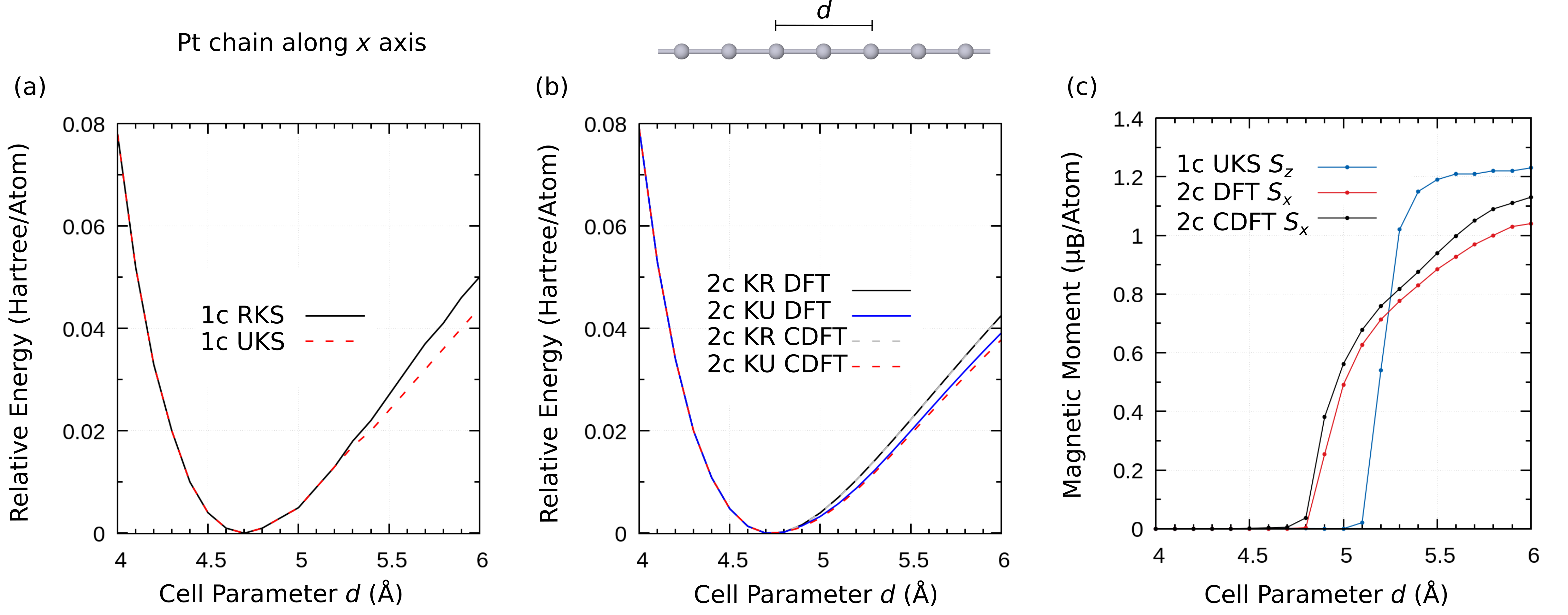
Figure 1: (a) Dependence of the energy on the cell parameter in units of Hartree per atom for one-component (1c) restricted Kohn–Sham (RKS) and 1c unrestriced Kohn–Sham (UKS) at the TPSS/dhf-SVP-2c level. (b) Dependence of the energy on the cell parameter in units of Hartree per atom for 2c KR and 2c KU with the spin aligned along $x$ ($S_{x}$). (c) Magnetic moment in units of Bohr’s magneton $\mu_{\textrm{B}}$ per atom for the spin contribution of 1c UKS, 2c KU $S_{x}$ DFT and CDFT approach. Periodicity is along the $x$ direction for one-dimensional systems. TURBOMOLE GmbH (2024a) The open-shell solutions are energetically favored compared to the respective closed-shell solutions and the $S_{x}$ alignment is preferred over $S_{y,z}$. Results without the current-independent TPSS functional are taken from Ref. 56. Detailed results are listed in the Supplementary Material.

The spin blocks of the Kohn–Sham equations are formed by combining the scalar and spin-magnetization contributions with the respective Pauli matrices, c.f. Refs.36 and 56. After transformation to the $k$ space, the Kohn–Sham equations can be solved as usual.

For non-magnetic or closed-shell system, $\vec{m}$ and $\vec{j}_{\text{p}}$ vanish so that a Kramers-restricted framework can be applied and time-reversal symmetry Kasper et al. (2020) may be exploited. However, the spin current densities are still non-zero and hence the spin-up and spin-down quantities $\vec{j}_{\uparrow,\downarrow}$ contribute to the XC potential through the diamagnetic or quadratic terms. Holzer, Franzke, and Pausch (2022)

The CDFT approach outlined herein is implemented in the riper module Burow, Sierka, and Mohamed (2009); Burow and Sierka (2011); Łazarski, Burow, and Sierka (2015); Łazarski et al. (2016); Grajciar (2015); Becker and Sierka (2019); Irmler, Burow, and Pauly (2018); Franzke, Schosser, and Pauly (2024) of TURBOMOLE. Ahlrichs et al. (1989); Franzke et al. (2023); TURBOMOLE GmbH (2024b) The numerical integration of the exchange-correlation potential is carried with the algorithm of Ref. 59. Note that the current density also leads to antisymmetric contributions. Integration weights are constructed according to Stratmann et al. Stratmann, Scuseria, and Frisch (1996) Geometry gradients and stress tensors are implemented based on previous work, as it essentially involves further derivatives of the basis functions. Łazarski et al. (2016); Becker and Sierka (2019); Franzke, Schosser, and Pauly (2024) We note that all integrals and the exchange potential for the Kohn–Sham equations are evaluated in the position space, which allows to exploit sparsity. The increase in the computational cost by calculating the current density contributions on a grid is modest—especially compared to the inclusion of the current density through Hartree–Fock exchange with hybrid functions.

III Computational Methods

First, we study the impact of the current density on the magnetic transition of one-dimensional linear Pt chains. Delin and Tosatti (2003, 2004); Fernández-Rossier et al. (2005); Smogunov et al. (2008); García-Suárez et al. (2009) Two Pt atoms are placed in the unit cell with the cell parameter $d$ ranging from 4.0 Å to 6.0 Å. Calculations are performed at the TPSS/dhf-SVP-2c Tao et al. (2003); Weigend and Baldes (2010) level employing Dirac–Fock effective core potentials (DF-ECPs), Figgen et al. (2009) replacing 60 electrons (ECP-60). A Gaussian smearing of 0.01 Hartree Kresse and Furthmüller (1996) is used and a $k$-mesh with 32 points is applied. Integration grids, convergence settings, etc.  are given in the Supplementary Material. We note in passing that the Karlsruhe dhf-type basis sets were optimized for discrete systems, Weigend and Baldes (2010) however, the corresponding pob-type basis sets for periodic calculations Peintinger, Oliveira, and Bredow (2013); Laun, Vilela Oliveira, and Bredow (2018); Vilela Oliveira et al. (2019); Laun and Bredow (2021, 2022); Seidler, Laun, and Bredow (2023) are not yet available with tailored extensions for spin–orbit two-component calculations. Armbruster, Klopper, and Weigend (2006) Therefore and for consistency with previous studies, we apply the dhf-type basis sets.

Second, the band gaps and the Rashba splitting of the transition-metal dichalcogenide monolayers MoCh₂ and WCh₂ (Ch = S, Se, Te) in the hexagonal (2H) phase are studied with the M06-L, Zhao and Truhlar (2006) r²SCAN, Furness et al. (2020a, b) TASK, Aschebrock and Kümmel (2019) TPSS, Tao et al. (2003) Tao–Mo, Tao and Mo (2016) and PKZB Perdew et al. (1999) functionals. The GGA PBE Perdew, Burke, and Ernzerhof (1996) serves as reference. The dhf-TZVP-2c basis set Weigend and Baldes (2010) is applied with DF-ECPs for Mo (ECP-28), W (ECP-60), Se (ECP-10), Te (ECP-28). Peterson et al. (2003, 2007); Figgen et al. (2009) Structures are taken from Ref. 93. A $k$-mesh of $33\crossproduct 33$ points is applied.

Third, the CDFT framework is applied to complement our previous meta-GGA study on silver halides. Franzke, Schosser, and Pauly (2024) Here, we consider the TPSS, Tao et al. (2003) revTPSS, Perdew et al. (2009, 2011) Tao–Mo, Tao and Mo (2016) PKZB, Perdew et al. (1999) r²SCAN, Furness et al. (2020a, b) and M06-L. Zhao and Truhlar (2006) We use the dhf-SVP basis set Weigend and Baldes (2010) and DF-ECPs are applied for Ag (ECP-28) and I (ECP-28). Figgen et al. (2005); Peterson et al. (2006) A $k$-mesh of $7\times 7\times 7$ is employed.

IV Results and Discussion

IV.1 Linear Pt Chain

The one-dimensional linear Pt chain is a common reference system for a transition to a magnetic system. The closed-shell configuration constitutes the electronic ground state with a small cell parameter, whereas the magnetic open-shell solution becomes lower in energy with increasing cell size. Delin and Tosatti (2003, 2004); Fernández-Rossier et al. (2005); Smogunov et al. (2008); García-Suárez et al. (2009) This is also confirmed at the scalar and spin–orbit TPSS level in Fig. 1. For small cell parameters from $d=4.0$ to $d=4.9$ Å, the open-shell initial guess converges to a closed-shell non-magnetic solution in the self-consistent field (SCF) procedure. The most favorable total energy is found for $d=4.7$ Å in agreement with previous studies based on GGA functionals. Smogunov et al. (2008); Franzke, Schosser, and Pauly (2024) Further, CDFT and DFT lead to a very similar potential energy surface or a similar behavior of the relative energy with respect to the cell parameter $d$.

At the scalar level, the transition to a magnetic material occurs between $d\approx 5.2$ Å and $d\approx 5.3$ Å. Inclusion of spin–orbit coupling shifts this transition to a smaller $d$ parameter of about $5.0$ Å. Here, the current-dependent variant of TPSS (cTPSS) leads to a lower total energy for both closed-shell and open-shell solutions, i.e. a more negative energy, and a larger magnetic moment. The impact of the current density is generally larger for the magnetic solution than for the closed-shell state, see also the Supplementary Material for detailed results. For the closed-shell solution, the difference in the total energy by inclusion of the current density is too small to be visible in panel (b) of Fig. 1. This finding is qualitatively in line with our previous studies on molecular systems. Holzer, Franzke, and Pausch (2022)

Inclusion of the current density also consistently leads to a larger magnetic moment. For instance, TPSS predicts a magnetic moment of 1.04 µ${}_{\text{B}}$/atom at $d=6.0$ Å, whereas a value of 1.13 µ${}_{\text{B}}$/atom is found with cTPSS. Generally, an increase in the range of 5–8 % is observed after the transition to a magnetic solution.

IV.2 Transition-Metal Dichalcogenide Monolayers

Transition-metal dichalcogenide monolayers have many interesting physical properties such as the quantum spin Hall, Liu, Feng, and Yao (2011) non-linear anomalous Hall, Kang et al. (2019) and Rashba effects. Zhu, Cheng, and Schwingenschlögl (2011) In the H2 phase, time-reversal symmetry holds for the non-magnetic systems but space-inversion symmetry is lost. Thus, spin–orbit coupling lifts the degeneracy of the valence band at the K point in the Brillouin zone. For the Mo and W systems, this Rashba splitting is very pronounced and values between 0.1 and 0.5 eV are obtained with relativistic all-electron methods. Miró, Audiffred, and Heine (2014); Kadek et al. (2023)

Table 1: Band gaps and Rashba splittings of the valence band at the K point for transition-metal dichalcogenide monolayers at the 1c DFT, 2c DFT, and 2c CDFT level with the dhf-TZVP-2c basis set and DF-ECPs for all atoms. All values in eV. Results for MoS₂ and WS₂ are listed in the Supplementary Material.

		Band Gap			Rashba Splitting
System	DFA	1c DFT	2c DFT	2c CDFT	2c DFT	2c CDFT
MoSe2	PBE	$1.554$	$1.453$	–	$0.166$	–
	PKZB	$1.558$	$1.455$	$1.455$	$0.166$	$0.169$
	Tao–Mo	$1.561$	$1.459$	$1.458$	$0.166$	$0.170$
	TPSS	$1.563$	$1.459$	$1.458$	$0.167$	$0.174$
	M06-L	$1.563$	$1.460$	$1.455$	$0.170$	$0.181$
	r2SCAN	$1.657$	$1.554$	$1.544$	$0.166$	$0.189$
	TASK	$1.735$	$1.629$	$1.607$	$0.172$	$0.218$
MoTe2	PBE	$1.157$	$1.039$	–	$0.185$	–
	PKZB	$1.160$	$1.042$	$1.042$	$0.186$	$0.189$
	Tao–Mo	$1.168$	$1.051$	$1.049$	$0.185$	$0.188$
	TPSS	$1.170$	$1.051$	$1.048$	$0.185$	$0.195$
	M06-L	$1.182$	$1.060$	$1.053$	$0.192$	$0.209$
	r2SCAN	$1.235$	$1.116$	$1.101$	$0.186$	$0.218$
	TASK	$1.287$	$1.161$	$1.126$	$0.197$	$0.269$
WSe2	PBE	$1.627$	$1.324$	–	$0.409$	–
	PKZB	$1.652$	$1.377$	$1.374$	$0.407$	$0.410$
	Tao–Mo	$1.667$	$1.371$	$1.367$	$0.403$	$0.411$
	TPSS	$1.660$	$1.379$	$1.371$	$0.409$	$0.420$
	M06-L	$1.668$	$1.413$	$1.405$	$0.422$	$0.440$
	r2SCAN	$1.774$	$1.482$	$1.452$	$0.419$	$0.457$
	TASK	$1.867$	$1.604$	$1.571$	$0.440$	$0.514$
WTe2	PBE	$1.219$	$0.933$	–	$0.423$	–
	PKZB	$1.227$	$0.953$	$0.951$	$0.423$	$0.427$
	Tao–Mo	$1.241$	$0.963$	$0.957$	$0.419$	$0.426$
	TPSS	$1.237$	$0.960$	$0.954$	$0.422$	$0.435$
	M06-L	$1.253$	$0.968$	$0.957$	$0.431$	$0.456$
	r2SCAN	$1.325$	$1.039$	$1.005$	$0.436$	$0.483$
	TASK	$1.388$	$1.096$	$1.050$	$0.465$	$0.566$

Band gaps and Rashba splittings at the K point obtained with DFT and CDFT approaches are listed in Tab. 1. One the one hand, the impact on the band gaps is rather small, with TASK and r²SCAN showing the largest changes but not exceeding 0.1 eV. Here, the deviation between the different DFAs is far larger. One the other hand, the Rashba splitting is very sensitive to the inclusion of the current density. For instance, the results change from 0.436 eV to 0.483 eV and 0.465 eV to 0.566 eV for WTe₂ with r²SCAN and TASK, respectively.

The most pronounced current-density effects are found for TASK throughout all systems, which is in line with molecular studies. Holzer, Franzke, and Pausch (2022); Bruder et al. (2023); Franzke and Holzer (2022) Here, the current density increase the Rashba splitting by 25 % on average. r²SCAN ranks second in this regard with 13 % followed by M06-L with 6 %. For PKZB, Tao–Mo and TPSS, changes of only 1–3 % are observed. Among the different monolayers, MoTe₂ leads to the largest impact of the current density for all DFAs, with a relative deviation of 36 % between DFT and CDFT for TASK. The impact of the current density for the DFAs can be rationalized by the enhancement factor. Franzke and Holzer (2022); Grotjahn, Furche, and Kaupp (2022)

IV.3 Silver Halide Crystals

Table 2: Optimized lattice constant $a$ (in Å, rocksalt structure) of three-dimensional AgI and band gaps (in eV) at high symmetry points of the first Brillouin zone with various density functional approximations and the dhf-SVP basis sets. A “c” indicates the current-dependent variant of the DFA. Results for DFAs without inclusion of the current density are taken from Ref. 56, except for M06-L. Calculations are performed without dispersion correction (no D3) and with the D3 correction using Becke–Johnson damping (D3-BJ).

DFA	Dispersion	$a$	L–L	–	X–X	L–X
TPSS	no D3	$6.153$	$3.249$	$2.047$	$2.937$	$0.583$
cTPSS	no D3	$6.150$	$3.244$	$2.052$	$2.940$	$0.579$
revTPSS	no D3	$6.116$	$3.149$	$2.132$	$2.998$	$0.537$
crevTPSS	no D3	$6.098$	$3.122$	$2.161$	$3.014$	$0.512$
Tao–Mo	no D3	$6.071$	$3.099$	$2.343$	$3.108$	$0.616$
cTao–Mo	no D3	$6.069$	$3.086$	$2.339$	$3.109$	$0.619$
PKZB	no D3	$6.200$	$3.409$	$2.153$	$2.987$	$0.826$
cPKZB	no D3	$6.210$	$3.422$	$2.138$	$2.979$	$0.839$
r2SCAN	no D3	$6.159$	$3.776$	$2.501$	$3.237$	$0.911$
cr2SCAN	no D3	$6.156$	$3.772$	$2.504$	$3.240$	$0.907$
M06-L	no D3	$6.325$	$3.511$	$1.891$	$2.976$	$1.116$
cM06-L	no D3	$6.327$	$3.512$	$1.889$	$2.974$	$1.117$
TPSS	D3-BJ	$5.982$	$2.988$	$2.352$	$3.098$	$0.343$
cTPSS	D3-BJ	$5.980$	$2.985$	$2.354$	$3.099$	$0.341$
revTPSS	D3-BJ	$5.949$	$2.883$	$2.443$	$3.156$	$0.291$
crevTPSS	D3-BJ	$5.952$	$2.889$	$2.435$	$3.152$	$0.296$
Tao–Mo	D3-BJ	$6.068$	$3.095$	$2.347$	$3.110$	$0.613$
cTao–Mo	D3-BJ	$6.062$	$3.087$	$2.358$	$3.116$	$0.604$
r2SCAN	D3-BJ	$6.156$	$3.773$	$2.506$	$3.240$	$0.907$
cr2SCAN	D3-BJ	$6.155$	$3.771$	$2.506$	$3.241$	$0.905$

The band gaps and optimized lattice constant of AgI with various meta-GGAs are listed in Tab. 2. Results for AgCl and AgBr are presented in the Supplementary Material. Overall, the current density is of minor importance for the band gaps. Changes are in the order of meV. These results are in qualitative agreement with the two-dimensional MoTe₂ monolayer, which consists of atoms from the same row of the periodic table of elements.

Likewise the current density does not lead to major changes for the cell structure and the lattice constant. The small impact on the lattice constant can be rationalized by the comparably small impact of spin–orbit coupling on the cell structure. Franzke, Schosser, and Pauly (2024) D3 dispersion correction with Becke–Johnson damping Grimme et al. (2010); Grimme, Ehrlich, and Goerigk (2011); Goerigk et al. (2017); Patra et al. (2020); Ehlert et al. (2021) (D3-BJ) leads to much larger changes than the application of CDFT. Therefore, other computational parameters than the inclusion of the current density for meta-GGAs are more important for the cell structures of the silver halide crystals.

V Conclusion

We have extended our previous formulation of spin–orbit current density functional theory to periodic systems of arbitrary dimension. The impact of the current density was assessed for various properties of non-magnetic and magnetic systems. Here, the band gaps and lattice constants are not notably affected. In contrast, the Rashba splitting which is only due to spin–orbit coupling is substantially affected. The inclusion of the current density for a given functional may lead to larger changes than the deviation of the results among different functionals.

With the present work, CDFT is now applicable to a wide range of chemical and physical properties of discrete and periodic systems, including analytic first-order property calculations. We generally recommend to include the current density for r²SCAN and the Minnesota functionals, if available in the used electronic structure code. For TASK, inclusion of the current density is clearly mandatory as it leads to substantial changes of the results.

Supplementary Material

Supporting Information is available with all computational details and data.

Author Declarations

Conflict of Interest

The authors have no conflicts to disclose.

Author Contributions

Yannick J. Franzke: Conceptualization (equal); Data curation (lead); Formal analysis (lead); Investigation (equal); Methodology (lead); Software (lead); Validation (equal); Visualization (lead); Writing – original draft (lead); Writing – review & editing (equal).
Christof Holzer: Conceptualization (equal); Data curation (supporting); Formal analysis (supporting); Investigation (equal); Methodology (supporting); Software (supporting); Validation (equal); Writing – original draft (supporting); Writing – review & editing (equal).

Data Availability Statement

The data that support the findings of this study are available within the article and its supplementary material.

References

in 1,…,0 See pages \x, of Supplementary-Material.pdf

References

- Burke (2012) K. Burke, J. Chem. Phys. 136, 150901 (2012).
- Becke (2014) A. D. Becke, J. Chem. Phys. 140, 18A301 (2014).
- Sun, Ruzsinszky, and Perdew (2015) J. Sun, A. Ruzsinszky, and J. P. Perdew, Phys. Rev. Lett. 115, 036402 (2015).
- Mardirossian and Head-Gordon (2017) N. Mardirossian and M. Head-Gordon, Mol. Phys. 115, 2315 (2017).
- Tao and Mo (2016) J. Tao and Y. Mo, Phys. Rev. Lett. 117, 073001 (2016).
- Hao et al. (2013) P. Hao, J. Sun, B. Xiao, A. Ruzsinszky, G. I. Csonka, J. Tao, S. Glindmeyer, and J. P. Perdew, J. Chem. Theory Comput. 9, 355 (2013).
- Mo et al. (2017) Y. Mo, R. Car, V. N. Staroverov, G. E. Scuseria, and J. Tao, Phys. Rev. B 95, 035118 (2017).
- Goerigk et al. (2017) L. Goerigk, A. Hansen, C. Bauer, S. Ehrlich, A. Najibi, and S. Grimme, Phys. Chem. Chem. Phys. 19, 32184 (2017).
- Franzke and Yu (2022a) Y. J. Franzke and J. M. Yu, J. Chem. Theory Comput. 18, 323 (2022a).
- Franzke and Yu (2022b) Y. J. Franzke and J. M. Yu, J. Chem. Theory Comput. 18, 2246 (2022b).
- Becke (2022) A. D. Becke, J. Chem. Phys. 156, 214101 (2022).
- Borlido et al. (2019) P. Borlido, T. Aull, A. W. Huran, F. Tran, M. A. L. Marques, and S. Botti, J. Chem. Theory Comput. 15, 5069 (2019).
- Holzer, Franzke, and Kehry (2021) C. Holzer, Y. J. Franzke, and M. Kehry, J. Chem. Theory Comput. 17, 2928 (2021).
- Holzer and Franzke (2022) C. Holzer and Y. J. Franzke, J. Chem. Phys. 157, 034108 (2022).
- Lee et al. (2021) J. Lee, X. Feng, L. A. Cunha, J. F. Gonthier, E. Epifanovsky, and M. Head-Gordon, J. Chem. Phys. 155, 164102 (2021).
- Ghosh et al. (2022) A. Ghosh, S. Jana, T. Rauch, F. Tran, M. A. L. Marques, S. Botti, L. A. Constantin, M. K. Niranjan, and P. Samal, J. Chem. Phys. 157, 124108 (2022).
- Kovás et al. (2022) P. Kovás, F. Tran, P. Blaha, and G. K. H. Madsen, J. Chem. Phys. 157, 094110 (2022).
- Liang et al. (2022) J. Liang, X. Feng, D. Hait, and M. Head-Gordon, J. Chem. Theory Comput. 18, 3460 (2022).
- Franzke (2023) Y. J. Franzke, J. Chem. Theory Comput. 19, 2010 (2023).
- Kovács, Blaha, and Madsen (2023) P. Kovács, P. Blaha, and G. K. H. Madsen, J. Chem. Phys. 159, 244118 (2023).
- Lebeda et al. (2023) T. Lebeda, T. Aschebrock, J. Sun, L. Leppert, and S. Kümmel, Phys. Rev. Mater. 7, 093803 (2023).
- Furness et al. (2015) J. W. Furness, J. Verbeke, E. I. Tellgren, S. Stopkowicz, U. Ekström, T. Helgaker, and A. M. Teale, J. Chem. Theory Comput. 11, 4169 (2015).
- Tellgren et al. (2014) E. I. Tellgren, A. M. Teale, J. W. Furness, K. K. Lange, U. Ekström, and T. Helgaker, J. Chem. Phys. 140, 034101 (2014).
- Irons, David, and Teale (2021) T. J. P. Irons, G. David, and A. M. Teale, J. Chem. Theory Comput. 17, 2166 (2021).
- Pausch and Holzer (2022) A. Pausch and C. Holzer, J. Phys. Chem. Lett. 13, 4335 (2022).
- Saue (2005) T. Saue, “Spin-interactions and the non-relativistic limit of electrodynamics,” in Advances in Quantum Chemistry, Vol. 48, edited by J. R. Sabin, E. Brändas, and L. B. Oddershede (Elsevier Academic Press, San Diego, CA, USA, 2005) pp. 383–405.
- Saue (2011) T. Saue, ChemPhysChem 12, 3077 (2011).
- Pyykkö (2012) P. Pyykkö, Annu. Rev. Phys. Chem. 63, 45 (2012).
- Dobson (1993) J. F. Dobson, J. Chem. Phys. 98, 8870 (1993).
- Tao (2005) J. Tao, Phys. Rev. B 71, 205107 (2005).
- Pittalis et al. (2007) S. Pittalis, S. Kurth, S. Sharma, and E. K. U. Gross, J. Chem. Phys. 127, 124103 (2007).
- Räsänen, Pittalis, and Proetto (2010) E. Räsänen, S. Pittalis, and C. R. Proetto, J. Chem. Phys. 132, 044112 (2010).
- Pittalis, Räsänen, and Gross (2009) S. Pittalis, E. Räsänen, and E. K. U. Gross, Phys. Rev. A 80, 032515 (2009).
- Bates and Furche (2012) J. E. Bates and F. Furche, J. Chem. Phys. 137, 164105 (2012).
- Maier, Ikabata, and Nakai (2020) T. M. Maier, Y. Ikabata, and H. Nakai, J. Chem. Phys. 152, 214103 (2020).
- Holzer, Franzke, and Pausch (2022) C. Holzer, Y. J. Franzke, and A. Pausch, J. Chem. Phys. 157, 204102 (2022).
- Desmarais et al. (2024a) J. K. Desmarais, G. Ambrogio, G. Vignale, A. Erba, and S. Pittalis, Phys. Rev. Mater. 8, 013802 (2024a).
- Desmarais et al. (2024b) J. K. Desmarais, J. Maul, B. Civalleri, A. Erba, G. Vignale, and S. Pittalis, arXiv (2024b), 10.48550/arXiv.2401.07581.
- Tellgren et al. (2012) E. I. Tellgren, S. Kvaal, E. Sagvolden, U. Ekström, A. M. Teale, and T. Helgaker, Phys. Rev. A 86, 062506 (2012).
- Becke (2002) A. D. Becke, J. Chem. Phys. 117, 6935 (2002).
- Kübler et al. (1988) J. Kübler, K.-H. Höck, J. Sticht, and A. R. Williams, J. Phys. F Metal Phys. 18, 469 (1988).
- Van Wüllen (2002) C. Van Wüllen, J. Comput. Chem. 23, 779 (2002).
- Saue and Helgaker (2002) T. Saue and T. Helgaker, J. Comput. Chem. 23, 814 (2002).
- Armbruster et al. (2008) M. K. Armbruster, F. Weigend, C. van Wüllen, and W. Klopper, Phys. Chem. Chem. Phys. 10, 1748 (2008).
- Peralta, Scuseria, and Frisch (2007) J. E. Peralta, G. E. Scuseria, and M. J. Frisch, Phys. Rev. B 75, 125119 (2007).
- Scalmani and Frisch (2012) G. Scalmani and M. J. Frisch, J. Chem. Theory Comput. 8, 2193 (2012).
- Bulik et al. (2013) I. W. Bulik, G. Scalmani, M. J. Frisch, and G. E. Scuseria, Phys. Rev. B 87, 035117 (2013).
- Baldes and Weigend (2013) A. Baldes and F. Weigend, Mol. Phys. 111, 2617 (2013).
- Egidi et al. (2017) F. Egidi, S. Sun, J. J. Goings, G. Scalmani, M. J. Frisch, and X. Li, J. Chem. Theory Comput. 13, 2591 (2017).
- Komorovsky, Cherry, and Repisky (2019) S. Komorovsky, P. J. Cherry, and M. Repisky, J. Chem. Phys. 151, 184111 (2019).
- Desmarais et al. (2021) J. K. Desmarais, S. Komorovsky, J.-P. Flament, and A. Erba, J. Chem. Phys. 154, 204110 (2021).
- Bruder, Franzke, and Weigend (2022) F. Bruder, Y. J. Franzke, and F. Weigend, J. Phys. Chem. A 126, 5050 (2022).
- Bruder et al. (2023) F. Bruder, Y. J. Franzke, C. Holzer, and F. Weigend, J. Chem. Phys. 159, 194117 (2023).
- Franzke et al. (2024) Y. J. Franzke, F. Bruder, S. Gillhuber, C. Holzer, and F. Weigend, J. Phys. Chem. A 128, 670 (2024).
- TURBOMOLE GmbH (2024a) TURBOMOLE GmbH, (2024a), manual of TURBOMOLE V7.8.1, a development of University of Karlsruhe and Forschungszentrum Karlsruhe GmbH, 1989-2007, TURBOMOLE GmbH, since 2007; available from https://www.turbomole.org/turbomole/turbomole-documentation/ (retrieved March 4, 2024).
- Franzke, Schosser, and Pauly (2024) Y. J. Franzke, W. M. Schosser, and F. Pauly, Phys. Rev. B (2024), 10.48550/arXiv.2305.03817, accepted.
- Kasper et al. (2020) J. M. Kasper, A. J. Jenkins, S. Sun, and X. Li, J. Chem. Phys. 153, 090903 (2020).
- Burow, Sierka, and Mohamed (2009) A. M. Burow, M. Sierka, and F. Mohamed, J. Chem. Phys. 131, 214101 (2009).
- Burow and Sierka (2011) A. M. Burow and M. Sierka, J. Chem. Theory Comput. 7, 3097 (2011).
- Łazarski, Burow, and Sierka (2015) R. Łazarski, A. M. Burow, and M. Sierka, J. Chem. Theory Comput. 11, 3029 (2015).
- Łazarski et al. (2016) R. Łazarski, A. M. Burow, L. Grajciar, and M. Sierka, J. Comput. Chem. 37, 2518 (2016).
- Grajciar (2015) L. Grajciar, J. Comput. Chem. 36, 1521 (2015).
- Becker and Sierka (2019) M. Becker and M. Sierka, J. Comput. Chem. 40, 2563 (2019).
- Irmler, Burow, and Pauly (2018) A. Irmler, A. M. Burow, and F. Pauly, J. Chem. Theory Comput. 14, 4567 (2018).
- Ahlrichs et al. (1989) R. Ahlrichs, M. Bär, M. Häser, H. Horn, and C. Kölmel, Chem. Phys. Lett. 162, 165 (1989).
- Franzke et al. (2023) Y. J. Franzke, C. Holzer, J. H. Andersen, T. Begušić, F. Bruder, S. Coriani, F. Della Sala, E. Fabiano, D. A. Fedotov, S. Fürst, S. Gillhuber, R. Grotjahn, M. Kaupp, M. Kehry, M. Krstić, F. Mack, S. Majumdar, B. D. Nguyen, S. M. Parker, F. Pauly, A. Pausch, E. Perlt, G. S. Phun, A. Rajabi, D. Rappoport, B. Samal, T. Schrader, M. Sharma, E. Tapavicza, R. S. Treß, V. Voora, A. Wodyński, J. M. Yu, B. Zerulla, F. Furche, C. Hättig, M. Sierka, D. P. Tew, and F. Weigend, J. Chem. Theory Comput. 19, 6859 (2023).
- TURBOMOLE GmbH (2024b) TURBOMOLE GmbH, (2024b), developers’ version of TURBOMOLE V7.8.1, a development of University of Karlsruhe and Forschungszentrum Karlsruhe GmbH, 1989-2007, TURBOMOLE GmbH, since 2007; available from https://www.turbomole.org (retrieved March 4, 2024).
- Stratmann, Scuseria, and Frisch (1996) R. Stratmann, G. E. Scuseria, and M. J. Frisch, Chem. Phys. 257, 213 (1996).
- Delin and Tosatti (2003) A. Delin and E. Tosatti, Phys. Rev. B 68, 144434 (2003).
- Delin and Tosatti (2004) A. Delin and E. Tosatti, Surf. Sci. 566–568, 262 (2004).
- Fernández-Rossier et al. (2005) J. Fernández-Rossier, D. Jacob, C. Untiedt, and J. J. Palacios, Phys. Rev. B 72, 224418 (2005).
- Smogunov et al. (2008) A. Smogunov, A. Dal Corso, A. Delin, R. Weht, and E. Tosatti, Nat. Nanotechnol. 3, 22 (2008).
- García-Suárez et al. (2009) V. M. García-Suárez, D. Z. Manrique, C. J. Lambert, and J. Ferrer, Phys. Rev. B 79, 060408(R) (2009).
- Tao et al. (2003) J. Tao, J. P. Perdew, V. N. Staroverov, and G. E. Scuseria, Phys. Rev. Lett. 91, 146401 (2003).
- Weigend and Baldes (2010) F. Weigend and A. Baldes, J. Chem. Phys. 133, 174102 (2010).
- Figgen et al. (2009) D. Figgen, K. A. Peterson, M. Dolg, and H. Stoll, J. Chem. Phys. 130, 164108 (2009).
- Kresse and Furthmüller (1996) G. Kresse and J. Furthmüller, Comput. Mater. Sci. 6, 15 (1996).
- Peintinger, Oliveira, and Bredow (2013) M. F. Peintinger, D. V. Oliveira, and T. Bredow, J. Comput. Chem. 34, 451 (2013).
- Laun, Vilela Oliveira, and Bredow (2018) J. Laun, D. Vilela Oliveira, and T. Bredow, J. Comput. Chem. 39, 1285 (2018).
- Vilela Oliveira et al. (2019) D. Vilela Oliveira, J. Laun, M. F. Peintinger, and T. Bredow, J. Comput. Chem. 40, 2364 (2019).
- Laun and Bredow (2021) J. Laun and T. Bredow, J. Comput. Chem. 42, 1064 (2021).
- Laun and Bredow (2022) J. Laun and T. Bredow, J. Comput. Chem. 43, 839 (2022).
- Seidler, Laun, and Bredow (2023) L. M. Seidler, J. Laun, and T. Bredow, J. Comput. Chem. 44, 1418 (2023).
- Armbruster, Klopper, and Weigend (2006) M. K. Armbruster, W. Klopper, and F. Weigend, Phys. Chem. Chem. Phys. 8, 4862 (2006).
- Zhao and Truhlar (2006) Y. Zhao and D. G. Truhlar, J. Chem. Phys. 125, 194101 (2006).
- Furness et al. (2020a) J. W. Furness, A. D. Kaplan, J. Ning, J. P. Perdew, and J. Sun, J. Phys. Chem. Lett. 11, 8208 (2020a).
- Furness et al. (2020b) J. W. Furness, A. D. Kaplan, J. Ning, J. P. Perdew, and J. Sun, J. Phys. Chem. Lett. 11, 9248 (2020b).
- Aschebrock and Kümmel (2019) T. Aschebrock and S. Kümmel, Phys. Rev. Res. 1, 033082 (2019).
- Perdew et al. (1999) J. P. Perdew, S. Kurth, A. c. v. Zupan, and P. Blaha, Phys. Rev. Lett. 82, 2544 (1999).
- Perdew, Burke, and Ernzerhof (1996) J. P. Perdew, K. Burke, and M. Ernzerhof, Phys. Rev. Lett. 77, 3865 (1996).
- Peterson et al. (2003) K. A. Peterson, D. Figgen, E. Goll, H. Stoll, and M. Dolg, J. Chem. Phys. 119, 11113 (2003).
- Peterson et al. (2007) K. A. Peterson, D. Figgen, M. Dolg, and H. Stoll, J. Chem. Phys. 126, 124101 (2007).
- Miró, Audiffred, and Heine (2014) P. Miró, M. Audiffred, and T. Heine, Chem. Soc. Rev. 43, 6537 (2014).
- Perdew et al. (2009) J. P. Perdew, A. Ruzsinszky, G. I. Csonka, L. A. Constantin, and J. Sun, Phys. Rev. Lett. 103, 026403 (2009).
- Perdew et al. (2011) J. P. Perdew, A. Ruzsinszky, G. I. Csonka, L. A. Constantin, and J. Sun, Phys. Rev. Lett. 106, 179902 (2011).
- Figgen et al. (2005) D. Figgen, G. Rauhut, M. Dolg, and H. Stoll, Chem. Phys. 311, 227 (2005).
- Peterson et al. (2006) K. A. Peterson, B. C. Shepler, D. Figgen, and H. Stoll, J. Phys. Chem. A 110, 13877 (2006).
- Liu, Feng, and Yao (2011) C.-C. Liu, W. Feng, and Y. Yao, Phys. Rev. Lett. 107, 076802 (2011).
- Kang et al. (2019) K. Kang, T. Li, E. Sohn, J. Shan, and K. F. Mak, Nature Materials 18, 324 (2019).
- Zhu, Cheng, and Schwingenschlögl (2011) Z. Y. Zhu, Y. C. Cheng, and U. Schwingenschlögl, Phys. Rev. B 84, 153402 (2011).
- Kadek et al. (2023) M. Kadek, B. Wang, M. Joosten, W.-C. Chiu, F. Mairesse, M. Repisky, K. Ruud, and A. Bansil, Phys. Rev. Mater. 7, 064001 (2023).
- Franzke and Holzer (2022) Y. J. Franzke and C. Holzer, J. Chem. Phys. 157, 031102 (2022).
- Grotjahn, Furche, and Kaupp (2022) R. Grotjahn, F. Furche, and M. Kaupp, J. Chem. Phys. 157, 111102 (2022).
- Grimme et al. (2010) S. Grimme, J. Antony, S. Ehrlich, and H. Krieg, J. Chem. Phys. 132, 154104 (2010).
- Grimme, Ehrlich, and Goerigk (2011) S. Grimme, S. Ehrlich, and L. Goerigk, J. Comput. Chem. 32, 1456 (2011).
- Patra et al. (2020) A. Patra, S. Jana, L. A. Constantin, and P. Samal, J. Chem. Phys. 153, 084117 (2020).
- Ehlert et al. (2021) S. Ehlert, U. Huniar, J. Ning, J. W. Furness, J. Sun, A. D. Kaplan, J. P. Perdew, and J. G. Brandenburg, J. Chem. Phys. 154, 061101 (2021).