Quantum Channel Simulation under Purified Distance is no more difficult than State Splitting

Abstract

Characterizing the minimal communication needed for the quantum channel simulation is a fundamental task in the quantum information theory. In this paper, we show that, under the purified distance, the quantum channel simulation can be directly achieved via quantum state splitting without using a technique known as the de Finetti reduction, and thus provide a pair of tighter one-shot bounds. Using the bounds, we also recover the quantum reverse Shannon theorem in a much simpler way.

I Introduction

We consider the problem of simulating a quantum channel using entanglement-assisted local operations and classical communications (eLOCC). We are interested in characterizing the minimal classical communication necessary for a faithful simulation of the channel measured under the purified distance. This is a fundamental task in quantum information theory, and the first-order asymptotic rate of the minimal classical communication is characterized by the entanglement-assisted capacity of the target channel, which is known as the reverse Shannon theorem [1, 2]. Recent years have seen a number of studies of the problem in different regimes, including the one-shot no-signaling-assisted regime [3], the moderate deviation regime [4], and network setups [5, 6].

However, despite the recent development, it remains an open task to characterize the asymptotic minimal rate of communication for quantum channel simulation in the second order. One of the major difficulties lies within the requirement that a channel simulation protocol must work for all input states simultaneously. This is in stark contrast with a highly related task known as the quantum state splitting (more precisely, a special case of the task known as the quantum state transfer). In particular, in both [4] and [6], the authors approached the problem of quantum channel simulation via the quantum state splitting of some so-called de Finetti state, at the cost of a multiplier before the deviation term $\epsilon$ that grows polynomially w.r.t. the blocklength $n$ (see, e.g., [4, Eq. (105]). This makes further studies of higher-order analyses very difficult along the same approach, if not impossible.

In this paper, we provide a much more direct relationship between the task of quantum state splitting and the quantum channel simulation. In particular, we show that the fidelity between the joint input-output density operators of the target channel and that of the simulated channel (see (1)) is quasi-convex w.r.t. the input density operator while concave w.r.t. to the protocol (as a CPTP map). Using Sion’s minimax theorem (see (2)), this implies that the protocol that works best for the worst input density operator has the same performance as the worst one among the protocols optimized for each input density operator. This finding not only provides a tighter one-shot achievability bound (cf. [4]), but also leads to a much simpler proof of the reverse Shannon theorem. Moreover, this opens up new possibilities for further studies on higher-order analyses of this problem.

In the following part of the paper, we first introduce the problem of quantum channel simulation and quantum state splitting together with suitable notations. Second, we show a direct connection between the two tasks, and thus provide a pair of tighter one-shot upper and lower bounds on the minimal message size for $\epsilon$-simulation of a quantum channel. Lastly, we recover the first-order asymptotic results, a.k.a. the quantum reverse Shannon theorem, using the newly found upper and lower bounds in a much simpler way.

II Quantum Channel Simulation and Quantum State Splitting

We hereby describe the task of simulating finite-dimensional quantum channels using entanglement-assisted local operations and classical communication. Suppose that we are given a quantum channel from system $\mathsf{A}$ to $\mathsf{B}$ described by some completely-positive-trace-preserving (CPTP) map $\mathcal{N}_{\mathsf{A}\to\mathsf{B}}:\mathcal{D}(\mathcal{H}_{\mathsf{A}})\to\mathcal{D}(\mathcal{H}_{\mathsf{B}})$ where the state spaces $\mathcal{H}_{\mathsf{A}}$ and $\mathcal{H}_{\mathsf{B}}$ are both finite-dimensional Hilbert spaces. We would like to find

• a pair of entangled systems $\mathsf{K}^{\prime}$ and $\mathsf{K}$ (with their joint state being some pure state $\left\lvert\sigma\right\rangle_{\mathsf{KK}^{\prime}}$),

• a local measurement on systems $\mathsf{A}$ and $\mathsf{K^{\prime}}$ (described by some POVM $\{E_{m}\}_{m\in[M]}$),

• a local operation from system $\mathsf{K}$ to $\mathsf{B}$ (described by some classical-controlled CPTP map $\Phi^{(m)}_{\mathsf{K}\to\mathsf{B}}$)

such that the joint effect of the latter two operations (which is a CPTP map from system $\mathsf{A}$ to $\mathsf{B}$), i.e.,

$$\widetilde{\mathcal{N}}_{\mathsf{A}\to\mathsf{B}}:\rho_{\mathsf{A}}\mapsto\sum_{m\in[M]}\Phi_{\mathsf{K}\to\mathsf{B}}^{(m)}\left(\operatorname{tr}_{\mathsf{AK^{\prime}}}\left[(E_{m}\otimes I_{\mathsf{K}})\cdot(\rho_{\mathsf{A}}\otimes\left\lvert\sigma\middle\rangle\!\middle\langle\sigma\right\rvert_{\mathsf{KK}^{\prime}})\right]\right)$$

resembles the channel $\mathcal{N}_{\mathsf{A}\to\mathsf{B}}$. This process is depicted in Figure 1.

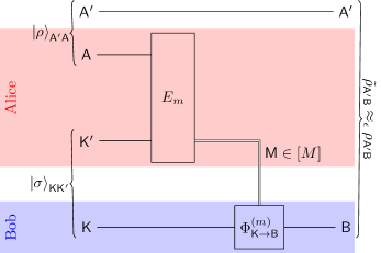
Figure 1: The task of quantum channel simulation with a tolerance of $\epsilon$ in the purified distance. The goal is to have $\widetilde{\rho}_{\mathsf{A}^{\prime}\mathsf{B}}\approx_{\epsilon}\rho_{\mathsf{A}^{\prime}\mathsf{B}}\coloneqq\operatorname{id}_{\mathsf{A}^{\prime}}\otimes\mathcal{N}_{\mathsf{A}\to\mathsf{B}}(\left\lvert\rho\middle\rangle\!\middle\langle\rho\right\rvert_{\mathsf{A}^{\prime}\mathsf{A}})$ for all input states $\rho_{\mathsf{A}}$, where $\left\lvert\rho\middle\rangle\!\middle\langle\rho\right\rvert_{\mathsf{A}^{\prime}\mathsf{A}}$ is the canonical purification of $\rho_{\mathsf{A}}$.

In particular, we are interested in finding the minimal alphabet size $M$ such that for all $\rho_{\mathsf{A}}\in\mathcal{D}(\mathcal{H}_{\mathsf{A}})$

$$F(\operatorname{id}_{\mathsf{A}^{\prime}}\otimes\mathcal{N}_{\mathsf{A}\to\mathsf{B}}(\left\lvert\rho\middle\rangle\!\middle\langle\rho\right\rvert_{\mathsf{A}^{\prime}\mathsf{A}}),\operatorname{id}_{\mathsf{A}^{\prime}}\otimes\widetilde{\mathcal{N}}_{\mathsf{A}\to\mathsf{B}}(\left\lvert\rho\middle\rangle\!\middle\langle\rho\right\rvert_{\mathsf{A}^{\prime}\mathsf{A}}))\geqslant 1-\epsilon^{2}$$ (1)

for some given $\epsilon\in(0,1)$. Here, $\mathsf{A}^{\prime}$ is a quantum system with the same state space as that of $\mathsf{A}$, and $\left\lvert\rho\middle\rangle\!\middle\langle\rho\right\rvert_{\mathsf{A}^{\prime}\mathsf{A}}\coloneqq(I_{\mathsf{A}^{\prime}}\otimes\sqrt{\rho_{\mathsf{A}}})\left\lvert\gamma\middle\rangle\!\middle\langle\gamma\right\rvert(I_{\mathsf{A}^{\prime}}\otimes\sqrt{\rho_{\mathsf{A}}})$ is the canonical purification of $\rho_{\mathsf{A}}$ on $\mathsf{A}^{\prime}$ where $\left\lvert\gamma\right\rangle$ is the maximal entangled state on the joint system $\mathsf{A}^{\prime}\mathsf{A}$. We use the following definition for the fidelity

$$F(\rho,\sigma)\coloneqq\left(\operatorname{tr}\sqrt{\rho^{1/2}\sigma\rho^{1/2}}\right)^{2}.$$

Quantum state splitting is a highly related task. In particular, quantum channel simulation can be seen as a “universal” version of the quantum state transfer, and the latter is a special case of quantum state splitting. Given some composite system $\mathsf{AB}$ with its state described by some known fixed density operator $\rho_{\mathsf{AB}}$, the task of quantum sate splitting is to send $\mathsf{B}$ from Alice to Bob using (one-way) classical communication and entanglement-assisted local operations, where at the beginning of the protocol Alice has access to both $\mathsf{A}$ and $\mathsf{B}$, and at the end of the protocol the joint density operator $\rho_{\mathsf{RAB}}^{\prime}$ is $\epsilon$ close to $\left\lvert\rho\middle\rangle\!\middle\langle\rho\right\rvert_{\mathsf{RAB}}$ in the purified distance, where $\mathsf{R}$ is some reference system that purifies $\mathsf{AB}$. This is illustrated in Fig. 2.

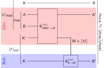
Figure 2: The task of quantum state splitting within a tolerance of $\epsilon$ in the purified distance. The goal is to have $\widetilde{\rho}_{\mathsf{RA}^{\prime}\mathsf{B}}\approx_{\epsilon}\left\lvert\rho_{\mathsf{RAB}}\middle\rangle\!\middle\langle\rho_{\mathsf{RAB}}\right\rvert$ where $\rho_{\mathsf{AB}}$ is fixed and known prior to the operations, and $\mathsf{R}$ is some reference system purifying $\mathsf{AB}$.

The major difference between the two tasks is that the protocols for the state splitting are $\rho_{\mathsf{AB}}$-specific; whereas the protocols for channel simulation have to work for all possible $\rho_{\mathsf{A}}$ with no knowledge or assumptions of it. In particular, the quantum channel simulation can be achieved by some universal state splitting protocol, i.e., a state splitting protocol that works for all possible $\rho_{\mathsf{AB}}$ (see Fig. 3). Without the “universality” of the state splitting protocol, say, we simply choose the best state splitting protocol for $\rho_{\mathsf{EB}^{\prime}}\coloneqq U_{\mathsf{AE}\to\mathsf{EB}}\cdot\left(\rho_{\mathsf{A}}\otimes\left\lvert 0\middle\rangle\!\middle\langle 0\right\rvert_{\mathsf{E}}\right)\cdot U_{\mathsf{AE}\to\mathsf{EB}}^{\dagger}$, the protocol in Fig. 3 only gives rise to a protocol as in Fig. 1 that only works for this specific $\rho_{\mathsf{A}}$.

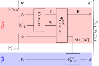
Figure 3: A quantum channel simulation protocol constructed from a state splitting protocol. Here, $U_{\mathsf{A}^{\prime}\mathsf{E}\to\mathsf{EB}^{\prime}}$ is the unitary representation of the original channel $\mathcal{N}_{\mathsf{A}^{\prime}\to\mathsf{B}^{\prime}}$. Note that we used the state splitting protocol on systems $\mathsf{E}$ and $\mathsf{B}^{\prime}$, and then discarded system $\mathsf{E}^{\prime}$.

For this very purpose, in the previous work [4], the state splitting protocols on the de Finetti state was considered when studying quantum channel simulations.

III Quantum Channel Simulation via State Splitting

In this section, we show that the expression in (1) is concave in $\widetilde{\mathcal{N}}_{\mathsf{A}\to\mathsf{B}}$ and quasi-convex in $\rho_{\mathsf{A}}$. This allows us to apply the Sion’s minimax theorem, and write

$$\adjustlimits{\sup}_{\widetilde{\mathcal{N}}_{\mathsf{A}\to\mathsf{B}}\in\mathfrak{P}_{\mathsf{A}\to\mathsf{B}}}{\inf}_{\rho_{\mathsf{A}}\in\mathcal{D}(\mathcal{H}_{\mathsf{A}})}F(\operatorname{id}_{\mathsf{A}^{\prime}}\otimes\mathcal{N}_{\mathsf{A}\to\mathsf{B}}(\left\lvert\rho\middle\rangle\!\middle\langle\rho\right\rvert_{\mathsf{A}^{\prime}\mathsf{A}}),\operatorname{id}_{\mathsf{A}^{\prime}}\otimes\widetilde{\mathcal{N}}_{\mathsf{A}\to\mathsf{B}}(\left\lvert\rho\middle\rangle\!\middle\langle\rho\right\rvert_{\mathsf{A}^{\prime}\mathsf{A}}))$$ (2)

$$= \adjustlimits{\inf}_{\rho_{\mathsf{A}}\in\mathcal{D}(\mathcal{H}_{\mathsf{A}})}{\sup}_{\widetilde{\mathcal{N}}_{\mathsf{A}\to\mathsf{B}}\in\mathfrak{P}_{\mathsf{A}\to\mathsf{B}}}F(\operatorname{id}_{\mathsf{A}^{\prime}}\otimes\mathcal{N}_{\mathsf{A}\to\mathsf{B}}(\left\lvert\rho\middle\rangle\!\middle\langle\rho\right\rvert_{\mathsf{A}^{\prime}\mathsf{A}}),\operatorname{id}_{\mathsf{A}^{\prime}}\otimes\widetilde{\mathcal{N}}_{\mathsf{A}\to\mathsf{B}}(\left\lvert\rho\middle\rangle\!\middle\langle\rho\right\rvert_{\mathsf{A}^{\prime}\mathsf{A}}))$$

where $\mathfrak{P}_{\mathsf{A}\to\mathsf{B}}$ is the set of all eLOCC protocols (formally defined below in (3)). In other words, under the same communication constraint, the best protocol for channel simulation has the same performance as the worst-performing protocol among the best protocols for each $\rho_{\mathsf{A}}$. This allows us to use the protocols derived from the state-splitting protocols (as in Fig. 3) and its achievability bounds (see [4, Theorem 3] and [7, Theorem 1]) to provide a one-shot achievability bound for the channel simulation. It is worth-noting that there are achievability bounds in network communication tasks that utilize the Sion’s minimax theorem in similar ways (e.g., see [8] and [9]). This bound matches with the converse bound (with small fudge terms) one can derive using the non-lockability property and the data-processing inequality of max-mutual information (e.g., see [4, Proposition 32]).

We formalize the set of all possible protocols as described at the beginning of this paper. Given quantum systems $\mathsf{A}$ and $\mathsf{B}$, we denote $\mathfrak{C}_{\mathsf{A}\to\mathsf{B}}$ the set of CPTP maps from $\mathsf{A}$ to $\mathsf{B}$, and we define the set of entanglement-assisted local-operation classical-communication (eLOCC) protocols from $\mathsf{A}$ to $\mathsf{B}$ with alphabet size $M\in\mathbb{N}$ as a subset of $\mathfrak{C}_{\mathsf{A}\to\mathsf{B}}$ as

$$\mathfrak{P}_{\mathsf{A}\to\mathsf{B}}^{(M)}\coloneqq\left\{\begin{aligned} &\widetilde{\mathcal{N}}_{\mathsf{A}\to\mathsf{B}}:\mathcal{D}(\mathcal{H}_{\mathsf{A}})\to\mathcal{D}(\mathcal{H}_{\mathsf{B}})\\ &\rho_{\mathsf{A}}\mapsto\sum_{m\in[M]}\Phi_{\mathsf{K}\to\mathsf{B}}^{(m)}\left(\operatorname{tr}_{\mathsf{AK^{\prime}}}\left[(E_{m}\otimes I_{\mathsf{K}})\cdot(\rho_{\mathsf{A}}\otimes\left\lvert\sigma\middle\rangle\!\middle\langle\sigma\right\rvert_{\mathsf{KK}^{\prime}})\right]\right)\end{aligned}\middle|\ \begin{aligned} &\mathsf{K}\text{, }\mathsf{K}^{\prime}\text{ are quantum systems with }\mathcal{H}_{\mathsf{K}}=\mathcal{H}_{\mathsf{K}}^{\prime}\\ &\{E_{m}\}_{m\in[M]}\text{ is some POVM on the joint system }\mathsf{AK}^{\prime}\\ &\Phi^{(m)}_{\mathsf{K}\to\mathsf{B}}\text{ is some CPTP from }\mathsf{K}\text{ to }\mathsf{B}\text{ for each }m\end{aligned}\right\}.$$ (3)

Notice that $\mathfrak{P}_{\mathsf{A}\to\mathsf{B}}^{(M)}$ is a convex (but not closed) subset of $\mathfrak{C}_{\mathsf{A}\to\mathsf{B}}$. To see $\mathfrak{P}_{\mathsf{A}\to\mathsf{B}}^{(M)}$ to be convex, we observe that any convex combination of two eLOCC protocols can be achieved using a single bit of shared randomness, i.e., Alice and Bob can choose to use protocol #1 if the bit turned out to be ‘0’, or protocol #2 if the bit is ‘1’. The shared randomness can be extracted from a pair of entangled qubits; and we only need to make the systems $\mathsf{K}$ and $\mathsf{K}^{\prime}$ larger.

For a given quantum channel $\mathcal{N}_{\mathsf{A}\to\mathsf{B}}$ from system $\mathsf{A}$ to system $\mathsf{B}$, the best performance (in terms of purified distance) of all $M$-alphabet-size eLOCC protocols for simulating $\mathcal{N}_{\mathsf{A}\to\mathsf{B}}$ can be expressed as

$$1-(\epsilon^{\star}_{M})^{2}=\adjustlimits{\sup}_{\widetilde{\mathcal{N}}_{\mathsf{A}\to\mathsf{B}}\in\mathfrak{P}_{\mathsf{A}\to\mathsf{B}}}{\inf}_{\rho_{\mathsf{A}}\in\mathcal{D}(\mathcal{H}_{\mathsf{A}})}F(\operatorname{id}_{\mathsf{A}^{\prime}}\otimes\mathcal{N}_{\mathsf{A}\to\mathsf{B}}(\left\lvert\rho\middle\rangle\!\middle\langle\rho\right\rvert_{\mathsf{A}^{\prime}\mathsf{A}}),\operatorname{id}_{\mathsf{A}^{\prime}}\otimes\widetilde{\mathcal{N}}_{\mathsf{A}\to\mathsf{B}}(\left\lvert\rho\middle\rangle\!\middle\langle\rho\right\rvert_{\mathsf{A}^{\prime}\mathsf{A}})).$$ (4)

Recall that $\mathcal{H}_{\mathsf{A}^{\prime}}=\mathcal{H}_{\mathsf{A}}$, and $\left\lvert\rho\middle\rangle\!\middle\langle\rho\right\rvert_{\mathsf{A}^{\prime}\mathsf{A}}\coloneqq(I_{\mathsf{A}^{\prime}}\otimes\sqrt{\rho_{\mathsf{A}}})\left\lvert\gamma\middle\rangle\!\middle\langle\gamma\right\rvert(I_{\mathsf{A}^{\prime}}\otimes\sqrt{\rho_{\mathsf{A}}})$ is the canonical purification of $\rho_{\mathsf{A}}$ on $\mathsf{A}^{\prime}$ where $\left\lvert\gamma\right\rangle$ is the maximal entangled state on the joint system $\mathsf{AA}^{\prime}$. We consider the following function

$$f:\mathfrak{P}_{\mathsf{A}\to\mathsf{B}}\times\mathcal{D}(\mathcal{H}_{\mathsf{A}}) \rightarrow\mathbb{R}_{\geqslant 0}$$ (5)

$$(\widetilde{\mathcal{N}}_{\mathsf{A}\to\mathsf{B}},\rho_{\mathsf{A}}) \mapsto\sqrt{F(\operatorname{id}_{\mathsf{A}^{\prime}}\otimes\mathcal{N}_{\mathsf{A}\to\mathsf{B}}((I_{\mathsf{A}^{\prime}}\otimes\sqrt{\rho_{\mathsf{A}}})\left\lvert\gamma\middle\rangle\!\middle\langle\gamma\right\rvert(I_{\mathsf{A}^{\prime}}\otimes\sqrt{\rho_{\mathsf{A}}})),\operatorname{id}_{\mathsf{A}^{\prime}}\otimes\widetilde{\mathcal{N}}_{\mathsf{A}\to\mathsf{B}}((I_{\mathsf{A}^{\prime}}\otimes\sqrt{\rho_{\mathsf{A}}})\left\lvert\gamma\middle\rangle\!\middle\langle\gamma\right\rvert(I_{\mathsf{A}^{\prime}}\otimes\sqrt{\rho_{\mathsf{A}}})))}.$$

Since the fidelity is a jointly concave function, the function $f$ defined above is also concave in its first argument $\widetilde{\mathcal{N}}_{\mathsf{A}\to\mathsf{B}}\in\mathfrak{P}_{\mathsf{A}\to\mathsf{B}}$ for each fixed $\rho_{\mathsf{A}}$. In the following, we show that the function $f$ is convex w.r.t. to its second argument $\rho_{\mathsf{A}}\in\mathcal{D}(\mathcal{H}_{\mathsf{A}})$.

Lemma 1.

The function $f$ defined in (4) is convex in $\rho_{\mathsf{A}}\in\mathcal{D}(\mathcal{H}_{\mathsf{A}})$ for each fixed $\widetilde{\mathcal{N}}_{\mathsf{A}\to\mathsf{B}}\in\mathfrak{P}_{\mathsf{A}\to\mathsf{B}}$.

Proof.

This can be shown as a direct result of [10, Proposition 4.80]. However, for completeness, we provide a short proof as follows. (An alternative proof is also included in Appendix A.)

Let $\widetilde{\mathcal{N}}_{\mathsf{A}\to\mathsf{B}}\in\mathfrak{P}_{\mathsf{A}\to\mathsf{B}}$ be fixed, and let $\rho_{0}\neq\rho_{1}\in\mathcal{D}(\mathcal{H}_{\mathsf{A}})$ be picked arbitrarily. For each $\lambda\in[0,1]$, denote $\rho_{\lambda}\coloneqq(1-\lambda)\cdot\rho_{0}+\lambda\cdot\rho_{1}$. Also denote $\left\lvert\rho_{\lambda}\right\rangle\coloneqq(I\otimes\sqrt{\rho_{\lambda}})\left\lvert\gamma\middle\rangle\!\middle\langle\gamma\right\rvert(I\otimes\sqrt{\rho_{\lambda}})$ the canonical purification of $\rho_{\lambda}$. Note that $\left\lvert\widetilde{\rho}_{\lambda}\right\rangle\coloneqq\sqrt{1-\lambda}\left\lvert 0\right\rangle\left\lvert\rho_{0}\right\rangle+\sqrt{\lambda}\left\lvert 1\right\rangle\left\lvert\rho_{1}\right\rangle$ is also a purification of $\rho_{\lambda}$. Therefore, denoting $\mathsf{R}$ a single-qubit auxiliary system, we have

$$f(\widetilde{\mathcal{N}}_{\mathsf{A}\to\mathsf{B}},\rho_{\lambda}) =F^{\frac{1}{2}}(\operatorname{id}_{\mathsf{A}^{\prime}}\otimes\mathcal{N}_{\mathsf{A}\to\mathsf{B}}(\left\lvert\rho_{\lambda}\middle\rangle\!\middle\langle\rho_{\lambda}\right\rvert),\operatorname{id}_{\mathsf{A}^{\prime}}\otimes\widetilde{\mathcal{N}}_{\mathsf{A}\to\mathsf{B}}(\left\lvert\rho_{\lambda}\middle\rangle\!\middle\langle\rho_{\lambda}\right\rvert))$$

$$=F^{\frac{1}{2}}(\operatorname{id}_{\mathsf{R}}\otimes\operatorname{id}_{\mathsf{A}^{\prime}}\otimes\mathcal{N}_{\mathsf{A}\to\mathsf{B}}(\left\lvert\widetilde{\rho}_{\lambda}\middle\rangle\!\middle\langle\widetilde{\rho}_{\lambda}\right\rvert),\operatorname{id}_{\mathsf{R}}\otimes\operatorname{id}_{\mathsf{A}^{\prime}}\otimes\widetilde{\mathcal{N}}_{\mathsf{A}\to\mathsf{B}}(\left\lvert\widetilde{\rho}_{\lambda}\middle\rangle\!\middle\langle\widetilde{\rho}_{\lambda}\right\rvert))$$ (6)

$$\leqslant\begin{aligned} F^{\frac{1}{2}}(\operatorname{id}_{\mathsf{R}}\otimes\operatorname{id}_{\mathsf{A}^{\prime}}\otimes\mathcal{N}_{\mathsf{A}\to\mathsf{B}}((1-\lambda)\left\lvert 0\middle\rangle\!\middle\langle 0\right\rvert\otimes\left\lvert\rho_{0}\middle\rangle\!\middle\langle\rho_{0}\right\rvert+\lambda\left\lvert 1\middle\rangle\!\middle\langle 1\right\rvert\otimes\left\lvert\rho_{1}\middle\rangle\!\middle\langle\rho_{1}\right\rvert),\ldots\\ \operatorname{id}_{\mathsf{R}}\otimes\operatorname{id}_{\mathsf{A}^{\prime}}\otimes\widetilde{\mathcal{N}}_{\mathsf{A}\to\mathsf{B}}((1-\lambda)\left\lvert 0\middle\rangle\!\middle\langle 0\right\rvert\otimes\left\lvert\rho_{0}\middle\rangle\!\middle\langle\rho_{0}\right\rvert+\lambda\left\lvert 1\middle\rangle\!\middle\langle 1\right\rvert\otimes\left\lvert\rho_{1}\middle\rangle\!\middle\langle\rho_{1}\right\rvert))\end{aligned}$$ (7)

$$=\begin{aligned} (1-\lambda)\cdot F^{\frac{1}{2}}(\operatorname{id}_{\mathsf{A}^{\prime}}\otimes\mathcal{N}_{\mathsf{A}\to\mathsf{B}}(\left\lvert\rho_{0}\middle\rangle\!\middle\langle\rho_{0}\right\rvert),\operatorname{id}_{\mathsf{A}^{\prime}}\otimes\widetilde{\mathcal{N}}_{\mathsf{A}\to\mathsf{B}}(\left\lvert\rho_{0}\middle\rangle\!\middle\langle\rho_{0}\right\rvert))+\ldots\\ \lambda\cdot F^{\frac{1}{2}}(\operatorname{id}_{\mathsf{A}^{\prime}}\otimes\mathcal{N}_{\mathsf{A}\to\mathsf{B}}(\left\lvert\rho_{1}\middle\rangle\!\middle\langle\rho_{1}\right\rvert),\operatorname{id}_{\mathsf{A}^{\prime}}\otimes\widetilde{\mathcal{N}}_{\mathsf{A}\to\mathsf{B}}(\left\lvert\rho_{1}\middle\rangle\!\middle\langle\rho_{1}\right\rvert))\end{aligned}$$

$$=(1-\lambda)\cdot f(\widetilde{\mathcal{N}}_{\mathsf{A}\to\mathsf{B}},\rho_{0})+\lambda\cdot f(\widetilde{\mathcal{N}}_{\mathsf{A}\to\mathsf{B}},\rho_{1})$$

where we use the Uhlmann’s theorem in (6), and measured the system $\mathsf{R}$ in (7). ∎

Lemma 1 provides a direct connection between the task of channel simulation and the state splitting. In particular, since the set $\mathcal{D}(\mathcal{H}_{\mathsf{A}})$ is closed and convex, and the set $\mathfrak{P}_{\mathsf{A}\to\mathsf{B}}$ is convex, we can apply the Sion’s minimax theorem, i.e.,

Theorem 2 (Sion’s minimax theorem [11]).

Let $\mathcal{X}$ be a compact convex set and $\mathcal{Y}$ be a convex set. If a function $f:\mathcal{X}\times\mathcal{Y}\to\mathbb{R}$ satiesfies

• $f(x,\cdot)$ is upper semi-continuous and quasi-concave on $\mathcal{Y}$ for each fixed $x\in\mathcal{X}$,

• $f(\cdot,y)$ is lower semi-continuous and quasi-convex on $\mathcal{X}$ for each fixed $y\in\mathcal{Y}$,

then,

$$\adjustlimits{\min}_{x\in\mathcal{X}}{\sup}_{y\in\mathcal{Y}}f(x,y)=\adjustlimits{\sup}_{y\in\mathcal{Y}}{\min}_{x\in\mathcal{X}}f(x,y).$$

Using the above theorem, we rewrite (4) as

$$1-(\epsilon^{\star}_{M})^{2}=\adjustlimits{\inf}_{\rho_{\mathsf{A}}\in\mathcal{D}(\mathcal{H}_{\mathsf{A}})}{\sup}_{\widetilde{\mathcal{N}}_{\mathsf{A}\to\mathsf{B}}\in\mathfrak{P}_{\mathsf{A}\to\mathsf{B}}}F(\operatorname{id}_{\mathsf{A}^{\prime}}\otimes\mathcal{N}_{\mathsf{A}\to\mathsf{B}}(\left\lvert\rho\middle\rangle\!\middle\langle\rho\right\rvert_{\mathsf{A}^{\prime}\mathsf{A}}),\operatorname{id}_{\mathsf{A}^{\prime}}\otimes\widetilde{\mathcal{N}}_{\mathsf{A}\to\mathsf{B}}(\left\lvert\rho\middle\rangle\!\middle\langle\rho\right\rvert_{\mathsf{A}^{\prime}\mathsf{A}})).$$ (8)

In other words, the optimal performance of channel simulations is directly determined by the optimal performance of quantum state transfers using eLOCC protocols under the same classical communication constraint. The latter can be achieved using quantum state-splitting protocols (see Fig. 3) provided that the message size $M$ is large enough [4].

Proposition 3.

Given a quantum channel $\mathcal{N}_{\mathsf{A}\to\mathsf{B}}$, there exists an eLOCC protocol with alphabet size $M$ that simulates $\mathcal{N}_{\mathsf{A}\to\mathsf{B}}$ within a tolerance of $\epsilon$ in the purified distance if

$$\log{M}\geqslant\adjustlimits{\sup}_{\rho_{\mathsf{A}}\in\mathcal{D}(\mathcal{H}_{\mathsf{A}})}{\inf}_{\sigma_{\mathsf{B}}\in\mathcal{D}(\mathcal{H}_{\mathsf{B}})}D_{\max}^{\epsilon-\delta,\mathsf{A}^{\prime}}\left(\rho_{\mathsf{A}^{\prime}\mathsf{B}}\middle\|\rho_{\mathsf{A}}\otimes\sigma_{\mathsf{B}}\right)-\log{\delta^{2}}$$ (9)

where $\rho_{\mathsf{A}^{\prime}\mathsf{B}}\coloneqq\operatorname{id}_{\mathsf{A}^{\prime}}\otimes\mathcal{N}_{\mathsf{A}\to\mathsf{B}}(\left\lvert\rho\middle\rangle\!\middle\langle\rho\right\rvert_{\mathsf{A}^{\prime}\mathsf{A}})$, and for density operators $\varrho_{\mathsf{AB}},\varsigma_{\mathsf{AB}}\in\mathcal{D}(\mathcal{H}_{\mathsf{AB}})$, and $\varepsilon\in(0,1)$, the partial smoothed max-divergence $D_{\max}^{\varepsilon,\mathsf{A}}\left(\varrho_{\mathsf{AB}}\middle\|\varsigma_{\mathsf{AB}}\right)$ is defined as

$$D_{\max}^{\varepsilon,\mathsf{A}}\left(\varrho_{\mathsf{AB}}\middle\|\varsigma_{\mathsf{AB}}\right)\coloneqq\inf_{\widetilde{\varrho}_{\mathsf{AB}}\in\mathcal{D}(\mathcal{H}_{\mathsf{AB}}):\widetilde{\varrho}_{\mathsf{A}}=\varrho_{\mathsf{A}},F(\widetilde{\varrho}_{\mathsf{AB}},\varrho_{\mathsf{AB}})\geqslant 1-\varepsilon^{2}}D_{\max}\left(\widetilde{\varrho}_{\mathsf{AB}}\middle\|\varsigma_{\mathsf{AB}}\right).$$

Proof.

This is a direct consequence of (8) and the results on the quantum state splitting (see [4, Theorem 3] and [7, Theorem 1]), i.e., given a pure state $\left\lvert\rho\right\rangle_{\mathsf{A}^{\prime}\mathsf{EB}^{\prime}}$, there exist a quantum state splitting protocol on systems $\mathsf{E}$ and $\mathsf{B}^{\prime}$ that achieves the $\epsilon$-tolerance in the purified distance if (note that $\rho_{\mathsf{A}}=\rho_{\mathsf{A}^{\prime}}$)

$$\log{M}\geqslant\inf_{\sigma_{\mathsf{B}}\in\mathcal{D}(\mathcal{H}_{\mathsf{B}})}D_{\max}^{\epsilon-\delta,\mathsf{A}^{\prime}}\left(\rho_{\mathsf{A}^{\prime}\mathsf{B}}\middle\|\rho_{\mathsf{A}^{\prime}}\otimes\sigma_{\mathsf{B}}\right)-\log{\delta^{2}}.$$ (10)

In other words, for an integer $M$ satisfying (9), for any $\rho_{\mathsf{A}}\in\mathcal{D}(\mathcal{H}_{\mathsf{A}})$, using the quantum state splitting protocol guaranteed to exists above, one can construct an eLOCC protocol $\widetilde{\mathcal{N}}_{\mathsf{A}\to\mathsf{B}}$ such that (see Fig. 3)

$$F(\operatorname{id}_{\mathsf{A}}\otimes\mathcal{N}_{\mathsf{A}^{\prime}\to\mathsf{B}}(\left\lvert\rho\middle\rangle\!\middle\langle\rho\right\rvert_{\mathsf{AA}^{\prime}}),\operatorname{id}_{\mathsf{A}}\otimes\widetilde{\mathcal{N}}_{\mathsf{A}^{\prime}\to\mathsf{B}}(\left\lvert\rho\middle\rangle\!\middle\langle\rho\right\rvert_{\mathsf{AA}^{\prime}}))\geqslant 1-\epsilon^{2}.$$

Referring to (8), the maximum fidelity that can be achieved by $M$-alphabet eLOCC protocols is at least

$$1-(\epsilon_{M}^{\star})^{2}\geqslant\inf_{\rho_{\mathsf{A}}\in\mathcal{D}(\mathcal{H}_{\mathsf{A}})}1-\epsilon^{2}=1-\epsilon^{2}.$$

Thus, there must exists at least one such protocol that simulates $\mathcal{N}_{\mathsf{A}\to\mathsf{B}}$ within the tolerance of $\epsilon$ in the purified distance. ∎

Similar to [4, Proposition 32] and [7, Theorem 2], we have the following one-shot converse bound.

Proposition 4.

Given a quantum channel $\mathcal{N}_{\mathsf{A}\to\mathsf{B}}$, for any $M$-alphabet-size eLOCC protocols that simulates $\mathcal{N}_{\mathsf{A}\to\mathsf{B}}$ within a tolerance of $\epsilon$ in purified distance, it holds that

$$\log{M}\geqslant\adjustlimits{\sup}_{\rho_{\mathsf{A}}\in\mathcal{D}(\mathcal{H}_{\mathsf{A}})}{\inf}_{\sigma_{\mathsf{B}}\in\mathcal{D}(\mathcal{H}_{\mathsf{B}})}D_{\max}^{\epsilon,\mathsf{A}^{\prime}}\left(\rho_{\mathsf{A}^{\prime}\mathsf{B}}\middle\|\rho_{\mathsf{A}}\otimes\sigma_{\mathsf{B}}\right),$$ (11)

where $\rho_{\mathsf{A}^{\prime}\mathsf{B}}\coloneqq\operatorname{id}_{\mathsf{A}^{\prime}}\otimes\mathcal{N}_{\mathsf{A}\to\mathsf{B}}(\left\lvert\rho\middle\rangle\!\middle\langle\rho\right\rvert_{\mathsf{A}^{\prime}\mathsf{A}})$.

Proof.

Suppose we have an eLOCC protocol with alphabet size $M$ that simulates the channel $\mathcal{N}_{\mathsf{A}\to\mathsf{B}}$. Let $\mathsf{M}$ denote the random variable representing the classical message (see Fig. 1). Starting from the picture of the systems right after the classical message $\mathsf{M}$ is gererated, we have the following chain of ineqalities

$$\log{M} =I_{\max}(\mathsf{A}^{\prime}:\mathsf{K})+\log{M}$$

$$\geqslant I_{\max}(\mathsf{A}^{\prime}:\mathsf{M}\mathsf{K})$$ (12)

$$\geqslant I_{\max}(\mathsf{A}^{\prime}:\mathsf{B})_{\widetilde{\rho}_{\mathsf{A}^{\prime}\mathsf{B}}}$$ (13)

where we used non-lockability of $I_{\max}$ (see [12, Cor. A.14]) in (12), and the data-processing inequality of $I_{\max}$ in (13), and we denote the density operator for systems $\mathsf{A}^{\prime}\mathsf{B}$ at the end of the protocol by $\widetilde{\rho}_{\mathsf{A}^{\prime}\mathsf{B}}$. Using the definition of $I_{\max}$, and the fact that $\widetilde{\rho}_{\mathsf{A}^{\prime}}=\rho_{\mathsf{A}}$, we have

$$I_{\max}(\mathsf{A}^{\prime}:\mathsf{B})_{\widetilde{\rho}_{\mathsf{A}^{\prime}\mathsf{B}}} =\inf_{\sigma_{\mathsf{B}}\in\mathcal{D}(\mathcal{H}_{\mathsf{B}})}D_{\max}\left(\widetilde{\rho}_{\mathsf{A}^{\prime}\mathsf{B}}\middle\|\rho_{\mathsf{A}}\otimes\sigma_{\mathsf{B}}\right)$$

$$\geqslant\inf_{\sigma_{\mathsf{B}}\in\mathcal{D}(\mathcal{H}_{\mathsf{B}})}D_{\max}^{\epsilon,\mathsf{A}^{\prime}}\left(\rho_{\mathsf{A}^{\prime}\mathsf{B}}\middle\|\rho_{\mathsf{A}}\otimes\sigma_{\mathsf{B}}\right),$$

where the last inequality is due to the guarantee from the protocol that $\widetilde{\rho}_{\mathsf{A}^{\prime}\mathsf{B}}$ is $\epsilon$-close to $\rho_{\mathsf{A}^{\prime}\mathsf{B}}$ in the purified distance. Combining the above, we know

$$\log{M}\geqslant\inf_{\sigma_{\mathsf{B}}\in\mathcal{D}(\mathcal{H}_{\mathsf{B}})}D_{\max}^{\epsilon,\mathsf{A}^{\prime}}\left(\rho_{\mathsf{A}^{\prime}\mathsf{B}}\middle\|\rho_{\mathsf{A}}\otimes\sigma_{\mathsf{B}}\right)$$

for any $\rho_{\mathsf{A}}\in\mathcal{D}(\mathcal{H}_{\mathsf{A}})$, which finishes the proof. ∎

IV First-Order Analysis

We now turn our attention to the asymptotic analysis of (9) and (11), i.e., the problem of simulating $n$ copies of the channel $\mathcal{N}_{\mathsf{A}\to\mathsf{B}}$. Note that this problem has already been solved as the quantum reverse Shannon theorem [1, 2], and we are merely recovering the result in a much simpler way.

For a fixed $\epsilon\in(0,1)$, let $M_{\epsilon}^{\star}(\mathcal{N}_{\mathsf{A}\to\mathsf{B}})$ denote the smallest alphabet size such that an eLOCC protocol can simulate $\mathcal{N}_{\mathsf{A}\to\mathsf{B}}$ within the tolerance of $\epsilon$ in the purified distance. We consider the asymptotics of the achievability bound first. Starting by applying Proposition 3 on $n$ copies of $\mathcal{N}_{\mathsf{A}\to\mathsf{B}}$, we have

$$\frac{1}{n}\log{M_{\epsilon}^{\star}(\mathcal{N}_{\mathsf{A}\to\mathsf{B}}^{\otimes n})}\leqslant\frac{1}{n}\adjustlimits{\sup}_{\rho_{\mathbf{\mathsf{A}}_{1}^{n}}\in\mathcal{D}(\mathcal{H}_{\mathbf{\mathsf{A}}_{1}^{n}})}{\inf}_{\sigma_{\mathbf{\mathsf{B}}_{1}^{n}}\in\mathcal{D}(\mathcal{H}_{\mathbf{\mathsf{B}}_{1}^{n}})}D_{\max}^{\epsilon-\delta,{\mathbf{\mathsf{A}}^{\prime}}_{1}^{n}}\left(\rho_{{\mathbf{\mathsf{A}}^{\prime}}_{1}^{n}\mathbf{\mathsf{B}}_{1}^{n}}\middle\|\rho_{\mathbf{\mathsf{A}}_{1}^{n}}\otimes\sigma_{\mathbf{\mathsf{B}}_{1}^{n}}\right)-\frac{1}{n}\log{\delta^{2}}$$

$$\hskip 25.0pt\leqslant\frac{1}{n}\adjustlimits{\sup}_{\rho_{\mathbf{\mathsf{A}}_{1}^{n}}\in\mathcal{D}(\mathcal{H}_{\mathbf{\mathsf{A}}_{1}^{n}})}{\inf}_{\sigma_{\mathbf{\mathsf{B}}_{1}^{n}}\in\mathcal{D}(\mathcal{H}_{\mathbf{\mathsf{B}}_{1}^{n}})}D_{\max}^{\frac{\epsilon-\delta-\delta^{\prime}}{2}}\left(\rho_{{\mathbf{\mathsf{A}}^{\prime}}_{1}^{n}\mathbf{\mathsf{B}}_{1}^{n}}\middle\|\rho_{\mathbf{\mathsf{A}}_{1}^{n}}\otimes\sigma_{\mathbf{\mathsf{B}}_{1}^{n}}\right)+\frac{1}{n}\log{\frac{8+\delta^{\prime 2}}{\delta^{\prime 2}}}-\frac{1}{n}\log{\delta^{2}}$$ (14)

$$\hskip 25.0pt=\frac{1}{n}\adjustlimits{\sup}_{\rho_{\mathbf{\mathsf{A}}_{1}^{n}}\in\mathcal{D}(\mathcal{H}_{\mathbf{\mathsf{A}}_{1}^{n}})}{\inf}_{\sigma_{\mathbf{\mathsf{B}}_{1}^{n}}\in\mathcal{D}(\mathcal{H}_{\mathbf{\mathsf{B}}_{1}^{n}})}D_{\max}^{\epsilon/4}\left(\rho_{{\mathbf{\mathsf{A}}^{\prime}}_{1}^{n}\mathbf{\mathsf{B}}_{1}^{n}}\middle\|\rho_{\mathbf{\mathsf{A}}_{1}^{n}}\otimes\sigma_{\mathbf{\mathsf{B}}_{1}^{n}}\right)+\frac{1}{n}\log{\frac{128+\epsilon^{2}}{\epsilon^{2}}}-\frac{1}{n}\log{\frac{\epsilon^{2}}{16}}$$ (15)

$$\hskip 25.0pt\leqslant\frac{1}{n}\underbrace{\adjustlimits{\sup}_{\rho_{\mathbf{\mathsf{A}}_{1}^{n}}\in\mathcal{D}(\mathcal{H}_{\mathbf{\mathsf{A}}_{1}^{n}})}{\inf}_{\sigma_{\mathbf{\mathsf{B}}_{1}^{n}}\in\mathcal{D}(\mathcal{H}_{\mathbf{\mathsf{B}}_{1}^{n}})}\widetilde{D}_{\alpha}\left(\rho_{{\mathbf{\mathsf{A}}^{\prime}}_{1}^{n}\mathbf{\mathsf{B}}_{1}^{n}}\middle\|\rho_{\mathbf{\mathsf{A}}_{1}^{n}}\otimes\sigma_{\mathbf{\mathsf{B}}_{1}^{n}}\right)}_{\eqqcolon\widetilde{I}_{\alpha}(\mathcal{N}_{\mathsf{A}\to\mathsf{B}}^{\otimes n})}+\underbrace{\frac{1}{n}\frac{-\log\left(1-\sqrt{1-\frac{\epsilon^{2}}{16}}\right)}{\alpha-1}+\frac{1}{n}\log{\frac{128+\epsilon^{2}}{\epsilon^{2}}}-\frac{1}{n}\log{\frac{\epsilon^{2}}{16}}}_{\to 0\text{ as }n\to\infty}$$ (16)

where in (14) we use [13, Theorem 11], in (15) we substitute $\delta,\delta^{\prime}\leftarrow\epsilon/4$, in (16) we use [14, Proposition 6.5]. Note that the sandwiched Rényi relative entropy is defined as

$$\widetilde{D}_{\alpha}\left(\rho\middle\|\sigma\right)\coloneqq\frac{1}{\alpha-1}\log{\operatorname{tr}\left(\sigma^{\frac{1-\alpha}{2\alpha}}\rho\sigma^{\frac{1-\alpha}{2\alpha}}\right)^{\alpha}}.$$

The first part of (16) is the sandwiched Rényi mutual information of the channel $\mathcal{N}_{\mathsf{A}\to\mathsf{B}}^{\otimes n}$ which is known to be additive [15, Lemma 6]; whereas the second part tends to zero as $n$ tends to infinity for any fixed $\alpha>1$ and $\epsilon\in(0,1)$. Thus, for all $\epsilon\in(0,1)$,

$$\limsup_{n\to\infty}\frac{1}{n}\log{M_{\epsilon}^{\star}(\mathcal{N}_{\mathsf{A}\to\mathsf{B}}^{\otimes n})} \leqslant\inf_{\alpha>1}\widetilde{I}_{\alpha}(\mathcal{N}_{\mathsf{A}\to\mathsf{B}})=\multiadjustlimits{\inf_{\alpha>1},\sup_{\rho_{\mathsf{A}}\in\mathcal{D}(\mathcal{H}_{\mathsf{A}})},\inf_{\sigma_{\mathsf{B}}\in\mathcal{D}(\mathcal{H}_{\mathsf{B}})}}\ \widetilde{D}_{\alpha}\left(\rho_{\mathsf{A}^{\prime}\mathsf{B}}\middle\|\rho_{\mathsf{A}}\otimes\sigma_{\mathsf{B}}\right)$$

$$\leqslant\multiadjustlimits{\inf_{\alpha>1},\sup_{\rho_{\mathsf{A}}\in\mathcal{D}(\mathcal{H}_{\mathsf{A}})},\inf_{\sigma_{\mathsf{B}}\in\mathcal{D}(\mathcal{H}_{\mathsf{B}})}}\ \left\{D\left(\rho_{\mathsf{A}^{\prime}\mathsf{B}}\middle\|\rho_{\mathsf{A}}\otimes\sigma_{\mathsf{B}}\right)+4(\alpha-1)(\log{v})^{2}\right\}$$ (17)

$$=\sup_{\rho_{\mathsf{A}}\in\mathcal{D}(\mathcal{H}_{\mathsf{A}})}I(\mathsf{A}:\mathsf{B})_{\rho_{\mathsf{AB}}}$$

where we use [16, Lemma 6.3] in (17), and $v$ is some constant for a given fixed channel $\mathcal{N}_{\mathsf{A}\to\mathsf{B}}$.

On the other hand, the asymptotics for the converse bound is relatively straightforward. By restricting the supreme over all input density operators $\rho_{\mathbf{\mathsf{A}}_{1}^{n}}$ to product states, we have

$$\frac{1}{n}\log{M_{\epsilon}^{\star}(\mathcal{N}_{\mathsf{A}\to\mathsf{B}}^{\otimes n})} \geqslant\frac{1}{n}\adjustlimits{\sup}_{\rho_{\mathbf{\mathsf{A}}_{1}^{n}}\in\mathcal{D}(\mathcal{H}_{\mathbf{\mathsf{A}}_{1}^{n}})}{\inf}_{\sigma_{\mathbf{\mathsf{B}}_{1}^{n}}\in\mathcal{D}(\mathcal{H}_{\mathbf{\mathsf{B}}_{1}^{n}})}D_{\max}^{\epsilon,{\mathbf{\mathsf{A}}^{\prime}}_{1}^{n}}\left(\rho_{{\mathbf{\mathsf{A}}^{\prime}}_{1}^{n}\mathbf{\mathsf{B}}_{1}^{n}}\middle\|\rho_{\mathbf{\mathsf{A}}_{1}^{n}}\otimes\sigma_{\mathbf{\mathsf{B}}_{1}^{n}}\right)$$

$$\geqslant\frac{1}{n}\adjustlimits{\sup}_{\rho_{\mathsf{A}}\in\mathcal{D}(\mathcal{H}_{\mathsf{A}})}{\inf}_{\sigma_{\mathbf{\mathsf{B}}_{1}^{n}}\in\mathcal{D}(\mathcal{H}_{\mathbf{\mathsf{B}}_{1}^{n}})}D_{\max}^{\epsilon,{\mathbf{\mathsf{A}}^{\prime}}_{1}^{n}}\left(\rho_{\mathsf{A}^{\prime}\mathsf{B}}^{\otimes n}\middle\|\rho_{\mathsf{A}}^{\otimes n}\otimes\sigma_{\mathbf{\mathsf{B}}_{1}^{n}}\right)$$

$$\eqqcolon\sup_{\rho_{\mathsf{A}}\in\mathcal{D}(\mathcal{H}_{\mathsf{A}})}\frac{1}{n}I_{\max}^{\epsilon,\mathrm{P}}(\dot{{\mathbf{\mathsf{A}}^{\prime}}_{1}^{n}}:\mathbf{\mathsf{B}}_{1}^{n})_{\rho_{\mathsf{A}^{\prime}\mathsf{B}}^{\otimes n}}\stackrel{{\scriptstyle\mathclap{\small\mbox{$n\to\infty$}}}}{{\xrightarrow{\hskip 56.9055pt}}}\sup_{\rho_{\mathsf{A}}\in\mathcal{D}(\mathcal{H}_{\mathsf{A}})}I(\mathsf{A}:\mathsf{B})_{\rho_{\mathsf{AB}}}$$

where in the last step above, we used the definition of the partial smoothed max-information (see [13, Eq. (11)]) and its asymptotic equipartition property (see [13, Eq. (107)], also see [14, Theorem 6.3]).

Summarizing the above discussion, we have the following theorem.

Theorem 5.

Let $\mathcal{N}_{\mathsf{A}\to\mathsf{B}}$ be a finite-dimensional quantum channel. For each $\epsilon\in(0,1)$, let $M_{\epsilon}^{\star}(\mathcal{N}_{\mathsf{A}\to\mathsf{B}})$ denote the smallest alphabet size $M$ such that there exists an $M$-alphabet-size eLOCC protocol that simulates $\mathcal{N}_{\mathsf{A}\to\mathsf{B}}$ within the tolerance of $\epsilon$ in the purified distance. It holds for any $\epsilon\in(0,1)$ that

$$\lim_{n\to\infty}\frac{1}{n}\log{M_{\epsilon}^{\star}}(\mathcal{N}_{\mathsf{A}\to\mathsf{B}}^{\otimes n})=\sup_{\rho_{\mathsf{A}}\in\mathcal{D}(\mathcal{H}_{\mathsf{A}})}I(\mathsf{A}^{\prime}:\mathsf{B})_{\rho_{\mathsf{A}^{\prime}\mathsf{B}}}\eqqcolon C_{\mathrm{E}}(\mathcal{N}_{\mathsf{A}\to\mathsf{B}}),$$

where $\rho_{\mathsf{A}^{\prime}\mathsf{B}}\coloneqq\operatorname{id}_{\mathsf{A}^{\prime}}\otimes\mathcal{N}_{\mathsf{A}\to\mathsf{B}}(\left\lvert\rho\middle\rangle\!\middle\langle\rho\right\rvert_{\mathsf{A}^{\prime}\mathsf{A}})$, and $\left\lvert\rho\middle\rangle\!\middle\langle\rho\right\rvert_{\mathsf{A}^{\prime}\mathsf{A}}\coloneqq(I_{\mathsf{A}^{\prime}}\otimes\sqrt{\rho_{\mathsf{A}}})\left\lvert\gamma\middle\rangle\!\middle\langle\gamma\right\rvert(I_{\mathsf{A}^{\prime}}\otimes\sqrt{\rho_{\mathsf{A}}})$.

Appendix A An Alternative Proof to Lemma 1

Proof.

Let $J$ and $\widetilde{J}$ be the Choi-Jamiolkowski state of the channel $\mathcal{N}_{\mathsf{A}\to\mathsf{B}}$ and $\widetilde{\mathcal{N}}_{\mathsf{A}\to\mathsf{B}}$, respectively, i.e.,

$$J\coloneqq\operatorname{id}_{\mathsf{A}^{\prime}}\otimes\mathcal{N}_{\mathsf{A}\to\mathsf{B}}\left(\left\lvert\gamma\middle\rangle\!\middle\langle\gamma\right\rvert_{\mathsf{A}^{\prime}\mathsf{A}}\right),\quad\widetilde{J}\coloneqq\operatorname{id}_{\mathsf{A}^{\prime}}\otimes\widetilde{\mathcal{N}}_{\mathsf{A}\to\mathsf{B}}\left(\left\lvert\gamma\middle\rangle\!\middle\langle\gamma\right\rvert_{\mathsf{A}^{\prime}\mathsf{A}}\right).$$

By writing (see [17, Eq. (19)])

$$\operatorname{id}_{\mathsf{A}^{\prime}}\otimes\mathcal{N}_{\mathsf{A}\to\mathsf{B}}(\left\lvert\rho\middle\rangle\!\middle\langle\rho\right\rvert_{\mathsf{A}^{\prime}\mathsf{A}}) =(\sqrt{\rho}\otimes I)\cdot J\cdot(\sqrt{\rho}\otimes I),$$

$$\operatorname{id}_{\mathsf{A}^{\prime}}\otimes\widetilde{\mathcal{N}}_{\mathsf{A}\to\mathsf{B}}(\left\lvert\rho\middle\rangle\!\middle\langle\rho\right\rvert_{\mathsf{A}^{\prime}\mathsf{A}}) =(\sqrt{\rho}\otimes I)\cdot\widetilde{J}\cdot(\sqrt{\rho}\otimes I),$$

we can rewrite (5) as

$$f:(\widetilde{\mathcal{N}}_{\mathsf{A}\to\mathsf{B}},\rho_{\mathsf{A}}) \mapsto\begin{aligned} \max\ &\frac{1}{2}\operatorname{tr}\left(Z+Z^{\dagger}\right)\\ \mathrm{s.t.}\ &\left(\begin{smallmatrix}(\sqrt{\rho}\otimes I)\cdot J\cdot(\sqrt{\rho}\otimes I)&Z\\ Z^{\dagger}&(\sqrt{\rho}\otimes I)\cdot\widetilde{J}\cdot(\sqrt{\rho}\otimes I)\end{smallmatrix}\right)\geqslant 0\end{aligned}$$

$$=\begin{aligned} \max\ &\frac{1}{2}\operatorname{tr}\left(Z+Z^{\dagger}\right)\\ \mathrm{s.t.}\ &(\sqrt{\rho}\otimes I)\cdot J\cdot(\sqrt{\rho}\otimes I)\geqslant Z\cdot(\sqrt{\rho}\otimes I)^{-1}\cdot\widetilde{J}^{-1}\cdot(\sqrt{\rho}\otimes I)^{-1}\cdot Z^{\dagger}\end{aligned}$$

$$=\begin{aligned} \max\ &\frac{1}{2}\operatorname{tr}\left(Z+Z^{\dagger}\right)\\ \mathrm{s.t.}\ &J\geqslant(\sqrt{\rho}\otimes I)^{-1}\cdot Z\cdot(\sqrt{\rho}\otimes I)^{-1}\cdot\widetilde{J}^{-1}\cdot(\sqrt{\rho}\otimes I)^{-1}\cdot Z^{\dagger}\cdot(\sqrt{\rho}\otimes I)^{-1}\end{aligned}$$

$$=\begin{aligned} \max\ &\frac{1}{2}\operatorname{tr}\left((\rho\otimes I)\cdot(\widetilde{Z}+\widetilde{Z}^{\dagger})\right)\\ \mathrm{s.t.}\ &J\geqslant\widetilde{Z}\cdot\widetilde{J}^{-1}\cdot\widetilde{Z}^{\dagger}\end{aligned}$$ (18)

where we substitute $\widetilde{Z}=(I\otimes\sqrt{\rho})^{-1}\cdot Z\cdot(I\otimes\sqrt{\rho})^{-1}$ in the last step. Note that (18) is a maximization over linear functions of $\rho$, and therefore much be convex in $\rho$. ∎

References

• [1] C. H. Bennett, P. W. Shor, J. A. Smolin, and A. V. Thapliyal, “Entanglement-assisted capacity of a quantum channel and the reverse Shannon theorem,” IEEE Transactions on Information Theory, vol. 48, no. 10, pp. 2637–2655, 2002.
• [2] C. H. Bennett, I. Devetak, A. W. Harrow, P. W. Shor, and A. Winter, “The quantum reverse Shannon theorem and resource tradeoffs for simulating quantum channels,” IEEE Transactions on Information Theory, vol. 60, no. 5, pp. 2926–2959, 2014.
• [3] K. Fang, X. Wang, M. Tomamichel, and M. Berta, “Quantum channel simulation and the channel’s smooth max-information,” IEEE Transactions on Information Theory, vol. 66, no. 4, pp. 2129–2140, 2019.
• [4] N. Ramakrishnan, M. Tomamichel, and M. Berta, “Moderate deviation expansion for fully quantum tasks,” IEEE Transactions on Information Theory, vol. 69, no. 8, pp. 5041–5059, 2023.
• [5] G. R. Kurri, V. Ramachandran, S. R. B. Pillai, and V. M. Prabhakaran, “Multiple access channel simulation,” IEEE Transactions on Information Theory, vol. 68, no. 11, pp. 7575–7603, 2022.
• [6] H.-C. Cheng, L. Gao, and M. Berta, “Quantum broadcast channel simulation via multipartite convex splitting,” arXiv preprint arXiv:2304.12056, 2023.
• [7] A. Anshu, V. K. Devabathini, and R. Jain, “Quantum communication using coherent rejection sampling,” Physical review letters, vol. 119, no. 12, p. 120506, 2017.
• [8] A. Anshu, M.-H. Hsieh, and R. Jain, “Noisy quantum state redistribution with promise and the alpha-bit,” IEEE Transactions on Information Theory, vol. 66, no. 12, pp. 7772–7786, 2020.
• [9] A. Anshu, R. Jain, and N. A. Warsi, “A hypothesis testing approach for communication over entanglement-assisted compound quantum channel,” IEEE Transactions on Information Theory, vol. 65, no. 4, pp. 2623–2636, 2018.
• [10] S. Khatri and M. M. Wilde, “Principles of quantum communication theory: A modern approach,” arXiv preprint arXiv:2011.04672, 2020.
• [11] M. Sion, “On general minimax theorems.” Pacific Journal of Mathematics, vol. 8, no. 1, pp. 171–176, 1958.
• [12] M. Berta, “Quantum side information: Uncertainty relations, extractors, channel simulations,” arXiv preprint arXiv:1310.4581, 2013.
• [13] A. Anshu, M. Berta, R. Jain, and M. Tomamichel, “Partially smoothed information measures,” IEEE Transactions on Information Theory, vol. 66, no. 8, pp. 5022–5036, 2020.
• [14] M. Tomamichel, Quantum information processing with finite resources: mathematical foundations.   Springer, 2015, vol. 5.
• [15] M. K. Gupta and M. M. Wilde, “Multiplicativity of completely bounded p-norms implies a strong converse for entanglement-assisted capacity,” Communications in Mathematical Physics, vol. 334, pp. 867–887, 2015.
• [16] M. Tomamichel, “A framework for non-asymptotic quantum information theory,” arXiv preprint arXiv:1203.2142, 2012.
• [17] Y. Ouyang, K. Goswami, J. Romero, B. C. Sanders, M.-H. Hsieh, and M. Tomamichel, “Approximate reconstructability of quantum states and noisy quantum secret sharing schemes,” Phys. Rev. A, vol. 108, p. 012425, Jul 2023. [Online]. Available: https://link.aps.org/doi/10.1103/PhysRevA.108.012425