Pensieve: Retrospect-then-Compare Mitigates Visual Hallucination

Abstract

Multi-modal Large Language Models (MLLMs) demonstrate remarkable success across various vision-language tasks. However, they suffer from visual hallucination, where the generated responses diverge from the provided image. Are MLLMs completely oblivious to accurate visual cues when they hallucinate? Our investigation reveals that the visual branch may simultaneously advocate both accurate and non-existent content. To address this issue, we propose Pensieve, a training-free method inspired by our observation that analogous visual hallucinations can arise among images sharing common semantic and appearance characteristics. During inference, Pensieve enables MLLMs to retrospect relevant images as references and compare them with the test image. This paradigm assists MLLMs in downgrading hallucinatory content mistakenly supported by the visual input. Experiments on Whoops [2], MME [10], POPE [28], and LLaVA Bench [35] demonstrate the efficacy of Pensieve in mitigating visual hallucination, surpassing other advanced decoding strategies. Additionally, Pensieve aids MLLMs in identifying details in the image and enhancing the specificity of image descriptions.

1 Introduction

Multi-modal Large Language Models (MLLMs) have emerged as dominant forces in vision-language tasks [34, 6, 67, 3, 31, 25, 24, 23, 40, 53, 57, 58, 61, 51], showcasing remarkable advancements in comprehending a wide array of visual concepts.

Despite their impressive capabilities, state-of-the-art MLLMs are susceptible to visual hallucination [33, 14, 15, 16, 22, 56, 66, 50, 44, 4, 43, 21, 32], wherein they inaccurately describe the visual inputs. Specifically, MLLMs can generate conflicting or fabricated content that diverges from the provided image, and may overlook crucial visual details. Examples illustrating this issue are presented in Fig. 1. Throughout this paper, we refer to the generated tokens (word or subword) containing inaccurate semantics as hallucinatory tokens.

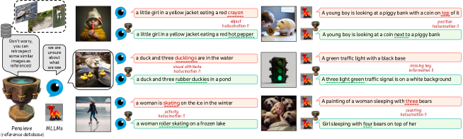
Figure 1: Visual hallucinations in image captions (marked in red) and an illustration of our proposed method Pensieve. MLLMs [34, 6] are enabled to retrospect relevant images as references and compare them with what they see. This methodology mitigates visual hallucinations, correcting errors in object category, visual attribute, activity, position, and counting. Pensieve also facilitates MLLMs to identify visual details in the image.

Understanding the origins of visual hallucinations is paramount for mitigation strategies. Previous studies underline flaws within MLLMs, such as under-distinctive visual features [44, 4], the image-text modality gap [15, 43], biased feature aggregation patterns [50, 14, 21], and fitting superficial language priors in the training data [66, 22, 32]. While these flaws can impede MLLMs from accurately comprehending images, our investigation suggests a different perspective: the MLLMs might not be entirely oblivious to accurate visual cues when they hallucinate; rather, they could be deceived by their eyes. We observe that the visual features tend to advocate both the accurate and non-existent token candidates, which we term visually deceptive candidates, by contributing close confidence scores to them (Sec. 3.1). This ambiguity can lead to visual hallucination (e.g., the hallucinatory token $\_fe$ in Fig. 2).

Eliciting accurate image descriptions from a non-blind MLLM is a crucial initial step in mitigating visual hallucination. We propose to downgrade the visually deceptive candidates by straightforwardly adjusting the predicted confidence scores. Commence with a premise that similar images are likely to induce analogous visual hallucinations, we step forward to analyze the confidence score distribution shift when replacing the test image with retrieved alternatives. We observe moderate changes in scores for visually deceptive candidates, whereas the scores for accurate token candidates exhibit more significant variations (Sec. 3.2). Leveraging this phenomenon, we introduce Pensieve, a training-free approach to mitigate visual hallucination. During inference, MLLMs are enabled to retrospect pertinent images as references and compare them with the test image. This novel retrospect-then-compare paradigm assists MLLMs in confirming accurate visual cues by emphasizing the difference between the test sample and the references (e.g., the rubber duckies in Fig. 1), thereby mitigating visual hallucination.

We validate Pensieve’s effectiveness in mitigating visual hallucination on image captioning and Visual Question Answering (VQA) tasks. Quantitative and qualitative results on four benchmarks (Whoops [2] in Tab. 1, LLaVA Bench in the wild [35] in Fig. 5, MME [10] in Tab. 2, and POPE [28] in Tab. 3) demonstrate that Pensieve outperforms other advanced decoding strategies [22, 5], effectively mitigating visual hallucination across various MLLMs [34, 6]. Additionally, Pensieve aids MLLMs in identifying details in the image (Fig. 1), avoiding specious responses (Fig. 4), and enhancing the specificity of descriptions (Fig. 5).

Our main contributions are three-fold: 1) We empirically unveil that MLLMs are not entirely clueless about the accurate visual concepts when they hallucinate, but faintly deceived by their eyes. 2) We introduce Pensieve, a novel paradigm that allows MLLMs to retrospect similar images during inference, and discern accurate visual cues through comparison. 3) Experiments on image captioning and VQA demonstrate the superiority of Pensieve in terms of mitigating visual hallucination, and enhancing the specificity of descriptions.

2 Related works

2.1 Visual Hallucination and their Origins

Visual hallucination [33] refers to the issue wherein the descriptive content diverges from the visual input. These erroneous responses may exhibit fabrication, contradictions, or scarce specificity to the provided image. Initial investigations primarily address object-level visual hallucination [41, 28, 66], focusing solely on inappropriate nouns. This problem is subsequently extended to a finer granularity [36, 49, 10, 43, 4, 48, 53, 44, 52, 16, 32], including errors in visual attributes, spatial relationships, physical states, activities, and numbers.

The origins of visual hallucination stem from various sources. Some highlight flaws in the visual branch, such as limited image resolution [59], under-distinctive visual representations that lack visual details [44] or spatial information [4], and poor cross-modal representation alignment [15]. Others emphasize deficiencies within the language model, such as biased attention score distributions [21, 50, 14], adherence to superficial syntactical patterns (e.g., frequent answers [32], contextual co-occurrence of objects [66, 22], and activities [52]), the overwhelming parametric knowledge [59], and error snowballing [60, 66, 52]. In this study, we extend the analytical method introduced in [29] to figure out what MLLMs see amidst visual hallucination, and find that they may not be completely blind to the faithful visual cues (Sec. 3.1). This observation suggests new perspectives that visual hallucination can be reduced without directly tackling MLLMs’ inherent deficiencies, which may incur extra labeling or training costs.

2.2 Mitigating Visual Hallucination

2.2.1 Parameter Tuning.

Effective methods include curating diverse multi-modal instruction tuning dataset [32, 58, 55] to bolster robustness, designing reward systems [43] to enhance multi-modal alignment, and the provision of extra supervisions [15, 4, 40, 57, 31, 3, 67] to foster visual comprehension. Nonetheless, the training cost becomes prohibitive for large-scale MLLMs. Furthermore, excessive parameter tuning may compromise MLLMs’ strengths, such as detailed description [32] and complex reasoning [4], when the training settings are suboptimal.

2.2.2 Model Ensemble.

Integrating knowledge from other models compensates for MLLMs’ shortcomings. Feasible methods include improving the object counting accuracy through detection models [56], prompting object recognition via segmentation masks [53, 58, 57, 61], and ensembling vision encoders for more distinctive image features [15, 31, 63]. Another line of work trains or prompts another language model to post hoc revise visual hallucinations [56, 66]. Key challenges within this paradigm include designing interfaces for various expert models, and automating their selection based on encountered problems.

2.2.3 Decoding Strategy.

Adjusting the confidence score distribution straightforwardly is a more efficient approach compared to model training and ensemble. OPERA [14] directly discards the candidates that may skew subsequent content toward hallucination and reelect the others. VCD [22] extends Contrastive Decoding (CD) [64, 27, 62, 42, 18, 5, 11], which aims to mitigate factual hallucinations in large language models (LLMs), to the vision domain. VCD uses a degraded image to suppress hallucinatory candidates that are plausible within the context. These strategies succeed in addressing syntactical biases within LLMs. However, they fall short in mitigating visually deceptive hallucinations (Sec. 3.1). In this study, we propose a training-free method Pensieve, which not only inherits the capability to counter MLLMs’ over-reliance on language priors [22] but also reduces hallucinations mistakenly advocated by the visual branch.

3 Delve into Visual Hallucination

3.0.1 Background.

Leading MLLMs [34, 6, 67, 57, 3, 31] incorporate auto-regressive language models [65, 45], which repeatedly selects the next token from their vocabulary $\mathcal{V}$ based on the probability of each token candidate $x_{i}$,

$$p_{\theta}(x_{i}|\boldsymbol{v},\boldsymbol{x},\boldsymbol{y}_{<t})=\frac{\exp{(\boldsymbol{h}_{t}\cdot E_{c}(x_{i})})}{\sum_{x^{\prime}\in V}\exp{(\boldsymbol{h}_{t}\cdot E_{c}(x^{\prime})})}$$ (1)

where $\boldsymbol{v}$ are the visual inputs, $\boldsymbol{x}$ and $\boldsymbol{y}_{<t}$ are the prompt and past generated tokens, respectively. $\boldsymbol{h}_{t}$ is the last hidden state predicted by the language model (also known as the next token feature). $E_{c}(x_{i})$ is the token embedding of candidate $x_{i}$ in the language head. $(\cdot)$ is the inner product operator. The confidence score $\boldsymbol{h}_{t}\cdot E_{c}(x_{i})$ embodies the degree of dominance of $x_{i}$’s semantics in $\boldsymbol{h}_{t}$.

3.0.2 Motivation.

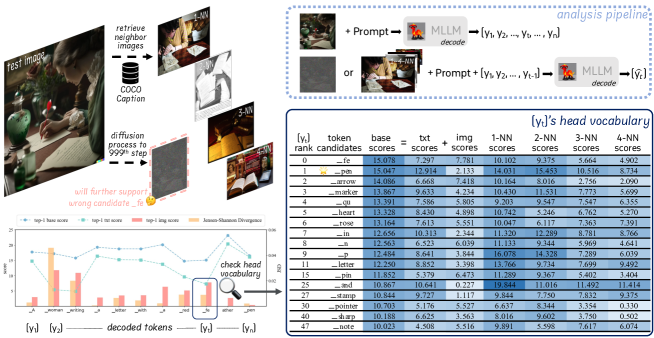
Figure 2: Analysis of visual hallucination through confidence score distribution. We investigate LLaVA1.5’s [34] predictions with alternative visual inputs within the same context. The model is not completely oblivious amidst visual hallucination, as the visual information contributed +7.418 scores for the accurate candidate $\_arrow$. However, the visual input also erroneously advocates for non-existent candidates (+7.781 scores for $\_fe$). We also observe that images with similar semantics and appearance can induce analogous visual hallucinations (e.g., $\_fe$, $\_pen$, and $\_marker$). We leverage this phenomenon to assist MLLMs in discerning the accurate content.

In this study, we pose the following questions: When visual hallucination occurs, are MLLMs completely ignorant about what they see? If they are not utterly blind, can we help them distinguish the accurate content from hallucinations? To address these inquiries, we aim to decouple the contribution of visual information in $\boldsymbol{v}$ to the predicted confidence scores. Inspired by [29], we first input the test images from [2] into the MLLM [34] and greedily decode tokens $[y_{1},\dots,y_{n}]$. At decoding step $t$, We denote $y_{t}$’s confidence score distribution as the base scores. Next, the test image is replaced with alternative images containing different visual information, and the predicted tokens thus far $[y_{1},\dots,y_{t-1}]$ are concatenated with $\boldsymbol{x}$ to predict $\hat{y_{t}}$. We anticipate the visual input shift $\Delta\boldsymbol{ve}$ to induce a corresponding output feature shift $\Delta\boldsymbol{h}$,

$$\Delta\boldsymbol{h}=\boldsymbol{h}_{t}-\hat{\boldsymbol{h}_{t}}$$ (2)

$$\boldsymbol{h}_{t}=LLM_{\theta}([VE(\boldsymbol{v});TE(\boldsymbol{x};\boldsymbol{y}_{<t})])$$ (3)

$$\hat{\boldsymbol{h}_{t}}=LLM_{\theta}([VE(\boldsymbol{v})-\Delta\boldsymbol{ve};TE(\boldsymbol{x};\boldsymbol{y}_{<t})])$$ (4)

$VE$ denotes the visual encoder and cross-modal connector. $TE$ is the text embedding layer. Therefore, the confidence score distribution shift $\Delta\boldsymbol{h}\cdot E_{c}(x^{\prime})$ for $x^{\prime}\in\mathcal{V}$ (i.e., the subtraction of $\hat{y_{t}}$’s confidence scores from $y_{t}$’s) represents the semantics in $\boldsymbol{h}_{t}$ contributed by the visual information in $\Delta\boldsymbol{ve}$.

3.1 MLLMs may not be Utterly Blind amidst Hallucination

To figure out what MLLMs see amidst visual hallucination, $\Delta\boldsymbol{ve}$ should encapsulate the majority of visual information present in the image. Hence, we diffuse [13] the test image until it is almost indistinguishable from Gaussian noise. The MLLM then predicts a new score distribution (the txt scores column in Fig. 2) devoid of valid visual cues. Consequently, the subtraction of the blindly predicted txt scores from the original base scores can be interpreted as the contribution of the visual modality (the img scores column in Fig. 2).

The example depicted in Fig. 2 exhibits multimodally distributed img scores across representative top-ranked candidates. Notably, both the accurate candidate (e.g., $\_arrow$) and numerous non-existent candidates (e.g., $\_fe$, $\_qu$ and $\_pin$) have relatively high img scores, indicating comparable advocacy from the visual branch. Therefore, the MLLM [34] is not completely blind to the accurate visual information when it hallucinates, but to some extent deceived by its eyes. We designate these non-existent candidates, which are mistakenly advocated by the visual input, as visually deceptive candidates. Conversely, candidates with limited support (or opposition) from the visual information are termed contextually deceptive candidates (e.g., $\_pen$, $\_in$ and $\_stamp$).

3.2 Visual References Help Distinguish Accurate Candidates

In the presence of both visually and contextually deceptive candidates, implementing VCD [22] (adding scaled img scores to base scores) will further elevate the score of the visually deceptive candidate $\_fe$, thereby exacerbating visual hallucination. We continue to explore feasible methods to help MLLMs discern this kind of erroneous content. Start with an intuitive hypothesis that within the same context $\boldsymbol{x}+\boldsymbol{y}_{<t}$, images sharing similar semantics and appearance are likely to induce analogous visual hallucinations, we proceed by analyzing the scores predicted using retrieved images, which possess visual characteristics in common with the test image. We present four retrieved images from COCO-Caption [30], with corresponding results in the k-NN scores columns in Fig. 2.

Upon comparing the base scores with the four k-NN scores, a notable observation emerges: the score of the faithful candidate $\_arrow$ decreases significantly, since the arrow appears only in the test image. In contrast, the alterations in scores for visually deceptive (e.g., $\_fe$ and $\_qu$) and contextually deceptive (e.g., $\_pen$ and $\_marker$) candidates, which are non-existent in any of the images, are relatively modest. This observation suggests the possibility of analogous visual hallucinations across similar images. We aim to leverage this phenomenon to aid MLLMs in distinguishing between accurate and hallucinatory content.

4 Methodology

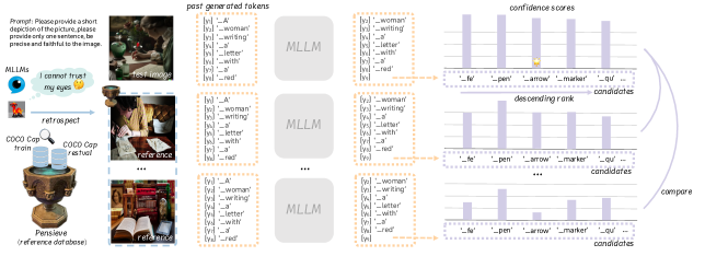
Figure 3: Our approach aims to identify non-existent candidates that are mistakenly supported by the visual input, by leveraging the analogous visual hallucinations among similar images. Our reference database comprises a variety of images, both familiar and unfamiliar to the model. During inference, MLLMs retrieve relevant references from this database and generate distinct predictions for each reference within the same context. The predicted scores are then compared to pinpoint the accurate candidates.

4.1 Retrospect Visual Concepts

We emphasize our motivation to discern visually deceptive content by leveraging analogous visual hallucinations among similar images (Sec. 3.2). Therefore, we anticipate the references to elicit visual hallucinations, while not unduly confusing the MLLMs. Additionally, the reference database should encompass a diverse range of visual concepts for versatility. Concretely, we construct the database with samples from the COCO Caption [30] Karpathy [17] train and restval splits, thereby covering a broad spectrum of common visual content. We posit that images from the restval split are more likely to induce visual hallucinations, as MLLMs[34, 6] have not seen them during the training process.

Specifically, MLLMs retrieve $k$ most relevant visual references for each test sample $q$ from a reference database $\mathcal{D}$, based on a similarity measure $\mathcal{F}(\cdot,\cdot)$,

$$\{r_{1},\dots,r_{k}|q\}=\underset{k}{\operatorname{arg\,max}}\{\mathcal{F}(E_{R}(s_{j}),E_{R}(q))|s_{j}\in\mathcal{D}\}\vspace{-0.1cm}$$ (5)

where $E_{R}(\cdot)$ is the retriever that embeds the raw inputs into representations. $\mathcal{D}[r],r\in\{r_{1},\dots,r_{k}|q\}$ are the desired references for $q$. In image captioning, the visual feature $E_{R}(\boldsymbol{v})$ is used to find images with similar semantics and appearance. In binary VQA, we adapt our approach to retrieve visual references that semantically align with the question using $E_{R}(\boldsymbol{x})$. We expect that comparing with such references will aid in reducing false positives.

4.2 Compare Visual Concepts

Contrasting with the confidence scores (denoted as logits in Eq. 6 and Eq. 9) predicted from visual references can help distinguish accurate visual cues. As illustrated in Fig. 3, the MLLM generates $k+2$ distinct predictions for each token candidate $x_{i}\in\mathcal{V}$ (from the test image $\boldsymbol{v}^{\tau}$, one diffused image $\boldsymbol{v}^{d}$, and $k$ retrieved images $\{\boldsymbol{v}^{NN}\}_{k}$) within the same context $\boldsymbol{x}+\boldsymbol{y}_{<t}$. We contrast $x_{i}$’s score corresponding to the test image $\boldsymbol{v}^{\tau}$ to $k+1$ references,

$$\mathit{logits}(x_{i}|\boldsymbol{x},\boldsymbol{y}_{<t},\boldsymbol{v}^{\tau},\boldsymbol{v}^{d},\{\boldsymbol{v}^{NN}\}_{k})$$

$$=(\alpha_{\tau}+\alpha_{d}^{t}+\alpha_{NN}^{t})\mathit{logits}(x_{i}|\boldsymbol{x},\boldsymbol{y}_{<t},\boldsymbol{v}^{\tau})$$

$$-\frac{\alpha_{NN}^{t}}{k}\sum_{j=1}^{k}\mathit{logits}(x_{i}|\boldsymbol{x},\boldsymbol{y}_{<t},\boldsymbol{v}^{NN}_{j})-\alpha_{d}^{t}\mathit{logits}(x_{i}|\boldsymbol{x},\boldsymbol{y}_{<t},\boldsymbol{v}^{d})$$ (6)

The subtraction operator in our paradigm underscores the difference between the test image and the visual references, thereby downgrading the analogous visual hallucinations across similar images. The retrieved images $\{\boldsymbol{v}^{NN}\}_{k}$ target at reducing visually deceptive content, and $\boldsymbol{v}^{d}$ aids in addressing contextually deceptive hallucinations [22]. The outcome of Eq. 6 is subsequently employed for token selection or sampling. This process repeats until the end of the sentence.

4.2.1 Adaptive Logits Processing.

We further extend the adaptive plausibility constraint [27] to regulate the influence of $\{\boldsymbol{v}^{NN}\}_{k}$ and $\boldsymbol{v}^{d}$. Specifically, in cases where MLLMs exhibit uncertainty [66] regarding the recognized visual cues, i.e., when the scores $\{l^{\delta}_{i,t}\}_{i=0}^{m-1}$ calculated by Eq. 9 demonstrate multimodal distribution, adjustments are made at decoding step $t$. The coefficient $\alpha_{d}^{t}$ is reduced while $\alpha_{NN}^{t}$ is increased. This adjustment ensures that the visually deceptive candidates are not further endorsed. Formally,

$$\alpha_{d}^{t}=\beta_{d}\exp{(\mathop{\max}(\mathrm{softmax}(\{l^{\delta}_{i,t}\}_{i=0}^{m-1})))}$$ (7)

$$\alpha_{NN}^{t}=\beta_{NN}\exp{(1-\mathop{\max}(\mathrm{softmax}(\{l^{\delta}_{i,t}\}_{i=0}^{m-1})))}$$ (8)

$$l^{\delta}_{i,t}=\mathit{logits}(x_{i}|\boldsymbol{x},\boldsymbol{y}_{<t},\boldsymbol{v}^{\tau})-\mathit{logits}(x_{i}|\boldsymbol{x},\boldsymbol{y}_{<t},\boldsymbol{v}^{d})\quad\text{s.t.}\quad x_{i}\in\mathcal{V}_{head}^{m}$$ (9)

where $x_{i}$ is within the top-ranked $m$ candidates, i.e., a fixed-length head vocabulary $\mathcal{V}_{head}^{m}$ [27], which is selected based on the scores predicted from $\boldsymbol{v}^{\tau}$. We set $m$ to 50 for image captioning and 2 for binary VQA. $\alpha_{\tau}$, $\beta_{d}$ and $\beta_{NN}$ are hyper-parameters (by default set to 1.0, 0.1, and 0.1, respectively).

5 Experiments

5.0.1 General Settings.

We evaluate Pensieve on image captioning (Whoops [2] in Tab. 1 and LLaVA-Bench [35] in Fig. 5) and VQA (MME [10] in Tab. 2 and POPE [28] in Tab. 3). The effectiveness of each component within Pensieve is examined in Tab. 4 and Fig. 6. All experiments are in zero-shot manner, with LLaVA1.5-7B [34] and InstructBLIP-7B [6] as baseline models, both using Vicuna [65] as the language decoder. We compare Pensieve with two advanced decoding strategies VCD [22] and DoLa [5]. To avoid hallucinations induced by token sampling [20, 26, 50], we employ greedy decoding as the baseline strategy. Implementation details and specific experimental settings are in the appendix.

5.1 Image Captioning

In light of that MLLMs encode rich real-world conventions and may fit certain superficial syntactical patterns in model parameters [22, 5, 66], we assume that commonsense-violating images (see Figs. 1 and 4) can highlight the problem of visual hallucination. For quantitative evaluation, image captioning metrics BLEU [38], METEOR [7], CIDEr [47], and SPICE [1] are employed. We utilize the FaithScore [16] for automatic visual hallucination evaluation, which is calculated via ChatGPT and a visual entailment expert model OFA [51]. We also provide qualitative results on LLaVA Bench in the Wild [35] (see Fig. 5) to illustrate the efficacy of Pensieve in real-world scenario comprehension.

5.1.1 Quantitative Results on Whoops.

Table 1: Results on Whoops [2] benchmark with commonsense-violating images. Pensieve boosts the overall performance for LLaVA-1.5 [34] and InstructBLIP [6]. B4, M, C, S, and FS% refer to Bleu@4, METEOR, CIDEr, SPICE (for image captioning), and FaithScore [16] (for visual hallucination), respectively. We copy the results of EVCap with and without retrieval augmentation (RA) from [23].

Method		B4 $\uparrow$	M $\uparrow$	C $\uparrow$	S $\uparrow$	FS% $\uparrow$
further trained on COCO
EVCap [23] Vicuna-13B		24.1	26.1	85.3	17.7	-
EVCap w/ RA [23] Vicuna-13B		24.4	26.1	86.3	17.8	-
zeroshot
LLaVA-1.5 [34] Vicuna-7B	greedy	19.7	25.6	67.9	17.3	67.9
	+DoLa	19.9	25.6	67.8	17.4	67.7
	+VCD	19.1	25.4	69.1	17.3	67.6
	+Ours	20.0	26.3	75.5	17.8	68.3
InstructBLIP [6] Vicuna-7B	greedy	24.9	26.5	87.3	18.2	74.1
	+DoLa	24.8	26.5	87.4	18.2	74.2
	+VCD	25.5	27.0	89.2	18.2	72.2
	+Ours	25.7	27.1	90.6	18.6	74.0

Tab. 1 demonstrate that our proposed Pensieve contributed to a substantial improvement in all captioning metrics for both MLLMs [34, 6], surpassing existing advanced decoding strategies [5, 22] in varying degrees. Although Pensieve promotes FaithScore [16] for LLaVA1.5 [34], a subtle drop is observed for InstructBLIP [6]. We provide qualitative results in Figs. 4 and 5 to validate Pensieve’s effectiveness in reducing visual hallucinations for InstructBLIP [6]. Furthermore, our retrospect-then-compare paradigm exhibits more pronounced improvements in image captioning performance compared to traditional retrieval-augmented (RA) image captioning paradigm [23], which relies on retrieved semantics to augment the input visual embeddings.

5.1.2 Qualitative Results on Whoops.

Figs. 1 and 4 illustrate the efficacy of our proposed Pensieve in mitigating visual hallucination, rectifying errors in object identification (such as the hot pepper and life preserver), visual attributes (including the rubber duckies, the color of the flowers and the Pokemon’s nose), activity recognition (notably identifying the roller-skating woman), spatial relationships (recognizing the coin is next to the piggy bank), and counting (identifying four bears). Whereas the impact of DoLa [5] is marginal, while VCD [22] can introduce extra visual hallucinations (e.g., the vase). Furthermore, Pensieve assists MLLMs in discerning nuanced visual cues in the images, such as the presence of three green lights on a traffic signal, flames coming out of a fire extinguisher, and the shadow belonging to another cat. Additionally, Pensieve prevents the generation of specious content (e.g., looking at the camera). We supplement these examples with two nearest neighbor references retrieved from [30], revealing that Pensieve-aided responses contain specific content appearing only in the test image. This evidence validates the superiority of Pensieve in mitigating visual hallucination, reducing specious responses, and identifying nuanced visual cues that even contradict common sense.

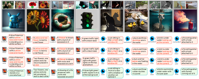
Figure 4: Qualitative Results on the Whoops [2] benchmark. Our proposed Pensieve effectively reduces visual hallucinations for both LLaVA-1.5 [34] and InstructBLIP [6], showcasing superiority over two advanced decoding strategies DoLa [5] and VCD [22]. Additionally, Pensieve demonstrates strengths in preventing specious text responses and identifying visual details, some of which may even violate common sense.

5.1.3 Qualitative Results on LLaVA Bench.

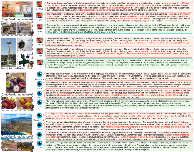
Figure 5: Qualitative results on LLaVA-Bench in the wild [35]. Our proposed Pensieve effectively mitigates visual hallucination for both LLaVA-1.5 [34] and InstructBLIP [6], with help of similar images from [30]. VCD [22] and DoLa [5] not only struggle to correct errors but may also induce extra hallucinations. Additionally, Pensieve enhances the specificity of generated responses by prompting MLLMs to spot the difference between the test image and the references. We omit DoLa’s responses in the upper two examples as they are identical to the original ones.

LLaVA Bench in the Wild [35] evaluates the ability of MLLMs to comprehend diverse visual concepts, spanning indoor and outdoor scenes, as well as comics. Fig. 5 demonstrate that Pensieve effectively reduces visual hallucinations for both MLLMs [34, 6], especially in the images that are crowded [53] with numerous objects (e.g., the refrigerator, the cityscape and the landscape). In these complex scenarios, VCD[22] and DoLa [5] struggle to assist MLLMs in discerning non-existent content, even inducing additional errors, such as misidentifying the edge of a table and boats. Moreover, Pensieve enhances MLLMs’ ability to capture distinctive visual cues and generate responses with heightened specificity (e.g., the accurate spatial relationship between the milk, the yogurt, and strawberries, and the smaller buildings scattered around the tower), meanwhile maintaining text fluency. We attribute this strength to the integration of visual references retrieved from [30], which enable MLLMs to validate accurate visual cues by identifying discrepancies.

5.2 Visual Question Answering

We further evaluate Pensieve on binary VQA benchmarks (MME [10] in Tab. 2 and POPE [28] in Tab. 3), which are designed to gauge the extent of visual hallucination in a yes-or-no discriminative manner. To prevent information leakage, we exclude all images that appeared in MME [10] and POPE [28] from the reference database, ensuring that the test samples do not serve as references.

5.2.1 Results on MME Benchmark.

Table 2: Results on the hallucination subset of the MME [10] benchmark, including the Color, Count, Existence, and Position subtasks, following [22]. We report the officially defined metric that combines accuracy and accuracy+. Pensieve elevates the total score for both MLLMs [34, 6]. More results are in the Appendix.

Model	Decoding	Color $\uparrow$	Count $\uparrow$	Exist. $\uparrow$	Pos. $\uparrow$	Total $\uparrow$
LLaVA-1.5	greedy	155.0	158.3	195.0	123.3	631.7
	+DoLa	153.3	158.3	195.0	123.3	630.0
	+VCD	148.3	158.3	190.0	126.7	623.3
	+Ours	165.0	153.3	195.0	128.3	641.7
InstructBLIP	greedy	120.0	60.0	185.0	50.0	415.0
	+DoLa	120.0	60.0	185.0	50.0	415.0
	+VCD	123.3	60.0	185.0	53.3	421.7
	+Ours	153.3	78.3	180.0	58.3	470.0

Following [56, 22], we present results on the Color, Count, Existence, and Position subtasks of MME [10] in Tab. 2. Our proposed Pensieve improves the total score for both LLaVA1.5 [34] and InstructBLIP [6], surpassing DoLa [5] and VCD [22] by a notable margin. Specifically, Pensieve effectively mitigates visual hallucination in color-related questions for both MLLMs. Besides, the position-related hallucinations in LLaVA1.5 [34] and the number-related hallucinations in InstructBLIP [6] are also reduced.

5.2.2 Results on POPE Benchmark.

Tab. 3 demonstrate that Pensieve boosts the accuracy of LLaVA1.5 [34], yet has a marginal impact on InstructBLIP [6]. Whereas DoLa [5] and VCD [22] deteriorate the performance of LLaVA1.5 [34] and InstructBLIP [6], respectively. It is worth noticing that greedy decoding avoids errors stemming from token sampling, thus significantly surpassing the multi-nominal sampling strategy reported in [22].

Table 3: Results on the POPE  [28] benchmark MSCOCO [30] dataset. We report the averaged performance on the random, popular, and adversarial settings.

Model	Decoding	Acc. $\uparrow$	Prec.	Rec.	F1 $\uparrow$
LLaVA-1.5	greedy	85.56	93.73	76.31	84.11
	+DoLa	85.38	93.82	75.84	83.86
	+VCD	85.59	86.51	84.71	85.53
	+Ours	85.80	92.82	77.73	84.58
InstructBLIP	greedy	85.14	89.06	80.40	84.45
	+DoLa	85.21	89.01	80.60	84.54
	+VCD	84.42	88.56	79.29	83.62
	+Ours	85.12	89.29	80.07	84.37

5.3 Ablation Studies

We validate the effectiveness of each component in Pensieve by individually ablating them. For quantitative evaluation, the image captioning metrics and the FaithScore [16] are employed (Tab. 4). We also investigate the impact of the reference database, varying its size through modifications in the source of visual references. Quantitative and qualitative results are present in Fig. 6.

Table 4: Ablation study on the WHOOPS [2] benchmark. Each component in Pensieve has a positive impact on the overall performance. All experiments are under the same hyperparameter setting, with LLaVA-v1.5-7B [34] as baseline MLLM (Exp.1). Results of our Pensieve are in Exp.2. Comparison to Exp.2 is marked in green or red.

Exp.	img. ret.	diffuse img.	comp.	adapt.	num. refs	B4 $\uparrow$	M $\uparrow$	C $\uparrow$	S $\uparrow$	FS% $\uparrow$
1					n/a	19.7	25.6	67.9	17.3	67.9
2	✓	✓	✓	✓	4	20.0	26.3	75.5	17.8	68.3
3	rand.	✓	✓	✓	4	$18.7^{\scalebox{0.6}{$\pm$0.3}}_{\scalebox{0.7}{({\color[rgb]{0,1,0}-1.3})}}$	$26.0^{\scalebox{0.6}{$\pm$0.1}}_{\scalebox{0.7}{({\color[rgb]{0,1,0}-0.3})}}$	$72.4^{\scalebox{0.6}{$\pm$0.7}}_{\scalebox{0.7}{({\color[rgb]{0,1,0}-3.1})}}$	$17.6^{\scalebox{0.6}{$\pm$0.1}}_{\scalebox{0.7}{({\color[rgb]{0,1,0}-0.2})}}$	$67.1^{\scalebox{0.6}{$\pm$0.3}}_{\scalebox{0.7}{({\color[rgb]{0,1,0}-1.2})}}$
4	✓		✓	✓	4	20.1 (+0.1)	26.2 (-0.1)	73.2 (-2.3)	17.9 (+0.1)	69.0 (+0.7)
5	✓	✓	add.	✓	4	17.6 (-2.4)	23.4 (-2.9)	58.7 (-16.8)	16.3 (-1.5)	66.9 (-1.4)
6	✓	✓	✓		4	19.9 (-0.1)	26.3 (-0.0)	71.9 (-3.6)	17.7 (-0.1)	68.9 (+0.6)
7	✓	✓	✓	✓	1	19.4 (-0.6)	26.3 (-0.0)	73.8 (-1.7)	17.5 (-0.3)	66.0 (-2.3)
8	✓	✓	✓	✓	2	19.8 (-0.2)	26.3 (-0.0)	74.6 (-0.9)	17.7 (-0.1)	67.5 (-0.8)
9	✓	✓	✓	✓	8	20.2 (+0.2)	26.4 (+0.1)	76.5 (+1.0)	17.9 (+0.1)	67.6 (-0.7)

5.3.1 Similar Images are better References.

We first ablate the image retrieval process (abbreviated img. ret.), randomly sampling four images from our database instead. The averaged results and the standard deviations from five separate runs are shown in Exp.3. The results indicate that random images could have positive impacts (compared to Exp.1), but similar images contribute to a more significant performance gain across all metrics (Exp.2). In Exp.4, we retain the retrieved images and discard the diffused image. Consequently, the faith score increased by 0.7 but the CIDEr metric noticeably dropped by 2.3. Additionally, we present the similarity metric used for image retrieval (the inner product score in Fig. 6, scaled and averaged on all test samples). Generally, higher similarity leads to better performance. These results underscore the superiority of similar images as references over random and diffused images.

5.3.2 Visual Concepts Comparison is Essential.

We alter the visual concept comparison step (abbreviated comp.), transitioning from logits subtraction (Eq. 6) to addition (i.e., emphasizing common visual cues present in both the test and reference images). Exp.5 demonstrates a notable decrease in all metrics, indicating that the additive paradigm can detrimentally affect the language modeling process. This result validates the necessity of contrasting visual concepts.

5.3.3 A Compact Reference Database is Sufficient.

We vary the size of the reference database by removing the images in the Karpathy [17] train or restval split in COCO Caption [30], or incorporating more images from the Visual Genome [19] dataset. Fig. 6 demonstrate that a database with up to 113k images can boost the overall performance, and enhance the specificity of generated responses. Notably, utilizing unseen references from the restval split yields the highest image captioning performance. Upon merging the two datasets [30, 19], we observe a decrease in the CIDEr metric, and more dissimilar content within the retrieved images. Consequently, there arises a necessity to bolster the robustness of the image retriever when scaling up the size of the reference database.

5.3.4 Other Ablations.

Exp.6 shows that the adaptive (abbreviated adapt.) logit processing scheme can enhance all metrics except for the FaithScore [16]. Besides, increasing the number of reference images provides steady improvement in the image captioning metrics (Exp.7-9). We use four references by default.

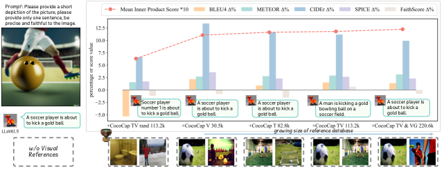
Figure 6: A compact reference database containing up to 113k reference images from COCO Caption [30] Karpathy [17] train (T) and restval (V) splits can improve performance across all metrics, and enhance the specificity of generated captions. Further scaling up the size of the reference database requires coordinated efforts to address potential noisy retrieval results. Overall, the performance gain positively correlates with the similarity between the test image and the references. The baseline result (depicted as the grey horizontal line) is Exp.1 in Tab. 4. Exp.2 corresponds to the setting +CocoCap TV 113.2k, and rand denotes sampling random references (Exp.3).

6 Limitation

Our proposed method Pensieve operates on the premise that within the same context, images with similar semantics and appearance are likely to induce analogous visual hallucinations. We provide qualitative evidence in Fig. 2 and in the appendix, but we find that quantitatively assessing the prevalence of this phenomenon is challenging. Nonetheless, our experiments demonstrate that this phenomenon can be leveraged to mitigate visual hallucination (Tabs. 1, 2 and 3). Besides, Pensieve introduces $\mathcal{O}(k)$ time complexity, as distinct confidence scores are predicted for each visual reference. The latency can be reduced by predicting reference confidence scores on multiple devices in parallel.

7 Conclusion

In this work, we address the visual hallucination issue of MLLMs, improving the trustworthiness of their depictions of the visual world. We conduct a detailed analysis to unveil that MLLMs may not be entirely blind to the accurate visual cues when they hallucinate, and similar images can induce analogous hallucinatory content. In light of this, we introduce a training-free method Pensieve, enabling MLLMs to respect similar images as references during inference, and to confirm the correct visual cues through comparison. This retrospect-then-compare paradigm particularly helps MLLMs discern non-existent content that is mistakenly supported by their visual branch. Quantitative and qualitative experiments on image captioning and visual question answering benchmarks validate the effectiveness of our proposed Pensieve in terms of visual hallucination mitigation, and enhancing the specificity of generated text responses.

Acknowledgment: This work is supported by the National Natural Science Foundation of China (No. 62372329), in part by the National Key Research and Development Program of China (No. 2021YFB2501104), in part by Shanghai Rising Star Program (No.21QC1400900), in part by Tongji-Qomolo Autonomous Driving Commercial Vehicle Joint Lab Project, and in part by Xiaomi Young Talents Program. We would like to acknowledge the discussions and comments for this project from Zehan Zheng.

Appendix 0.A Explanations for our Analysis Pipeline

0.A.1 Semantics in the Last Hidden State

We denote $E_{c}(x_{i})$ as the token embedding of candidate $x_{i}$ in the language model head, where $E_{c}(\cdot)$ embeds token $x_{i}$ into a feature vector with hidden dimension $d$. The embeddings of all candidates (the total number is the length of the model’s vocabulary $length(\mathcal{V})$) form the weight matrix in the language model head, which is a linear projection layer without dropout, activate function, or bias. The confidence score at decoding step $t$ corresponding to candidate $x_{i}$ is determined by the inner product of its embedding $E_{c}(x_{i})$ and the last hidden state $\boldsymbol{h}_{t}$ predicted by the MLLM. When the confidence scores of different candidates are proximate, as illustrated in Figs. 9, 10, 11, 12, 13, 14 and 15, $\boldsymbol{h}_{t}$ reflects a blend of diverse semantics in near-equal proportions. Consequently, these close confidence scores yield low probabilities following the $\mathrm{softmax}$ operation, indicating that MLLMs exhibit uncertainty in their current prediction.

Following our analysis pipeline (Sec. 3.0.2), if the score shift $\Delta\boldsymbol{h}\cdot E_{c}(x_{i})$ corresponding to candidate $x_{i}$ is a positive value, then $\Delta\boldsymbol{h}$ strengthens the semantics associated with $x_{i}$. Conversely, certain semantics may be attenuated by $\Delta\boldsymbol{h}$ (e.g., the candidate $\_yellow$ in Fig. 15 receives a negative img score). When the score shift is close to zero, we infer that $\Delta\boldsymbol{h}$ is orthogonal to $E_{c}(x_{i})$.

0.A.2 Quantify MLLMs’ Blindness

We utilize the Jensen-Shannon Divergence (JSD) to quantify MLLMs’ blindness during text decoding. Specifically, JSD is calculated between the confidence scores predicted by the test image $\boldsymbol{v}^{\tau}$ and those from the diffused image $\boldsymbol{v}^{d}$ in the same context $\boldsymbol{x}+\boldsymbol{y}_{<t}$. The calculation is performed within the head vocabulary $\mathcal{V}_{head}^{m}$, comprising the top-ranked $m$ candidates. Formally,

$$\mathrm{JSD}(P\parallel Q)=\frac{1}{2}\left(D_{KL}(P\parallel M)+D_{KL}(Q\parallel M)\right)$$ (10)

$$M=\frac{1}{2}(P+Q)$$ (11)

$$P=\mathrm{softmax}(\{\mathit{logits}(x_{j}|\boldsymbol{x},\boldsymbol{y}_{<t},\boldsymbol{v}^{\tau})|x_{j}\in\mathcal{V}_{head}^{m}\})$$ (12)

$$Q=\mathrm{softmax}(\{\mathit{logits}(x_{j}|\boldsymbol{x},\boldsymbol{y}_{<t},\boldsymbol{v}^{d})|x_{j}\in\mathcal{V}_{head}^{m}\})$$ (13)

where $D_{KL}(\cdot)$ is the Kullback-Leibler (KL) divergence. A high JSD value indicates differences between the probability distributions calculated from the two score distributions (i.e., the base scores and the txt scores) by the $\mathrm{softmax}$ operation. Consequently, the subtraction of the of txt scores from the base scores (i.e., the img scores) is not uniformly distributed, suggesting that some (but not all) candidates are advocated by the visual input. Conversely, when both the JSD and the first place candidate’s img score (denoted as the top-1 img score) are close to zero, the visual information hardly influences the prediction (i.e., contributes few scores) at the current decoding step. In other words, the MLLM is blind. The provided examples in Figs. 2, 10, 11, 12, 13, 14 and 15 reveal that in a sentence, the JSD values of erroneous nouns and adjectives are relatively higher compared to articles, conjunctions, and subwords. This observation suggests that MLLMs may not be utterly blind amidst visual hallucination.

Appendix 0.B Implementation Details

0.B.1 Details for Visual Retrospection

0.B.1.1 Image Retrievers.

For image captioning, the retriever extracts semantic and appearance features from visual inputs $\boldsymbol{v}$. CLIP [39] ViT [8] demonstrates strength in encoding visual semantics, while the self-supervised pretrained DINOv2[37] excels in capturing finer visual details [44]. We use CLIP [39] and DINOv2 [37] ViT-L14 models. For bin VQA, CLIP [39] Transformer [46] extracts semantics from the input question $\boldsymbol{x}$. We aim to find visual references that semantically align with $\boldsymbol{x}$, thereby we do not add image representations here considering that they may perturb the semantics in $E_{R}(\boldsymbol{x})$. Before encoding $\boldsymbol{x}$, we modify the question templates used in MME [10] and POPE [28] to transform questions into narratives (e.g., replacing the string Is there with A photo of).

0.B.1.2 Similarity Metrics.

$\mathcal{F}(\cdot,\cdot)$ is the cosine similarity. The representations are L2 normalized before the Maximum Inner Product Search (MIPS) conducted by FAISS [9], which is a library for vector similarity search and clustering. For image captioning, we concatenate the $[cls]$ tokens from CLIP [39] and DINOv2 [37] ViTs, equally weighting the semantic and appearance similarities. For VQA on the MME [10] benchmark, we re-order the retrieval results based on the BLEU@1 [38] score between the query and the retrieved captions.

0.B.2 Details for Visual Comparison

If not otherwise specified, we denote the rank as the ordering of candidates according to the base scores predicted using the test image $\boldsymbol{v}^{\tau}$. At decoding step $t$, we establish a cut-off confidence score equal to the base score of the $m^{th}$-ranked candidate. Confidence scores below this threshold are set to $-float(inf)$. Therefore, candidates outside the head vocabulary $\mathcal{V}_{head}^{m}$ are excluded from consideration, both in greedy decoding and token sampling processes.

0.B.2.1 Compare when Necessary.

The JSD value can approach zero in certain decoding steps, particularly for subwords (e.g., $ck$ and $lings$ after $\_du$ in Fig. 10), and lexical collocations (e.g., $\_being$ after $\_is$ and $\_of$ after $\_middle$ in Fig. 14). Modifying the confidence score distribution for these cases might adversely affect the language modeling process. To address this issue, a JSD threshold can be optionally set to deactivate Pensieve in such decoding steps.

Appendix 0.C Experiments

0.C.1 Detailed Experimental Settings

0.C.1.1 Datasets and Metrics.

On POPE [28] (Polling-based Object Probing Evaluation) and MME [10], the MLLMs are prompted to answer yes or no with one word. Based on whether the response contains the string $yes$ or $no$, the Accuracy, Precision, Recall, and F1 score are determined on POPE [28], the summation of Accuracy and Accuracy$+$ are calculated on MME [10]. For image captioning, we evaluate our proposed Pensieve on two challenging benchmarks: the Whoops [2] benchmark (comprising 500 generated images with high-fidelity, and some of the visual cues in those images may violate common sense) and the LLaVA Bench in the Wild [35] (abbreviated as $LLaVA^{W}$, containing 60 questions posed on 24 images, including indoor and outdoor scenes, memes, paintings, and sketches).

For visual hallucination evaluation on the Whoops [2] and ${LLaVA}^{W}$ [35] benchmarks, we employ the FaithScore [16] metric, which is capable of assessing nuanced visual hallucinations and exhibits a stronger correlation with human judgment than traditional metrics like CHAIR [41] and CLIP-Score [12]. We utilize the gpt-3.5-turbo-1106 API along with the model OFA [51] (the finetuned version on the visual entailment dataset SNLI-VE [54]). We deviate from models in the LLaVA or BLIP family, as we are evaluating LLaVA-1.5 [34] and InstructBLIP[6]. Throughout our experiments, we query ChatGPT three times and report the averaged results.

0.C.1.2 Hyper-parameters.

We list the hyper-parameters used in our experiments in Tab. 5. The official code implementation of DoLa [5] and VCD [22] are utilized. For DoLa, we adopt the dynamic premature layer selection strategy, with the argument $mature\_layer$ set to 32, $premature\_layer$ to a list $[0,2,4,6,8,10,12,14]$, and $relative\_top$ to 0.1. Regarding VCD, we adhere to the officially established hyper-parameters on MME [10] and POPE [28] benchmarks ($cd\_alpha=1$, $cd\_beta=0.1$, the diffusion step is set to 500 for MME [10] and 999 for POPE [28]). However, we observe that setting VCD’s $cd\_alpha=1$ on the Whoops [2] and $LLaVA^{W}$ [35] benchmarks could impair the fluency of generated captions. Consequently, we reduced it to 0.1.

Table 5: Detailed hyper-parameter settings for LLaVA-1.5 [34] and InstructBLIP [6] for each test dataset. diffu. step denotes the image diffusion step.

Model	Hyper-param.	Whoops [2]	LLaVAW [35]	MME [10]	POPE [28]
LLaVA-1.5	$k$	4	2	1	2
	$\beta_{NN}$	0.1	0.1	0.01	0.05
	$\beta_{d}$	0.1	0.1	0.1	0.01
	$\alpha_{\tau}$	1.0	1.0	1.0	1.0
	diffu. step	900	900	700	900
InstructBLIP	$k$	2	2	2	2
	$\beta_{NN}$	0.04	0.1	0.1	0.02
	$\beta_{d}$	0.05	0.1	0.5	0.02
	$\alpha_{\tau}$	1.2	1.0	1.0	1.5
	diffu. step	500	900	900	900

0.C.1.3 MLLM Baselines.

We select two representative MLLMs [34, 6] to implement our method. Both MLLMs integrate CLIP-ViT [39] as the visual encoder. As for the cross-modal connector, LLaVA-1.5 [34] uses a two-layer MLP, and InstructBLIP [6] uses a Q-former [24] with textual input.

0.C.1.4 Settings for the Ablation Study.

For all ablation studies, we utilize LLaVA-1.5-7B [34] as the baseline MLLM, maintaining the default hyper-parameter settings consistent with the experiments on Whoops [2] in Tab. 1. In ablation study Exp.4, we set $\beta_{d}=1e-6$ to neutralize the impact of the diffused image $\boldsymbol{v}^{d}$ on confidence score processing. However, we retain the diffused image itself, as it remains necessary for calculating $\alpha_{NN}^{t}$. In Exp.6, both $\alpha_{d}^{t}$ and $\alpha_{NN}^{t}$ are fixed at 0.1. In the study of the reference database size, we incorporate all 108k images from the Visual Genome [19] dataset.

0.C.2 More Results on LLaVA Bench in the Wild

We present more qualitative results to demonstrate the effectiveness of our proposed Pensieve in Fig. 7. Pensieve adeptly corrects visual hallucinations that pose challenges for both DoLa [5] and VCD [22], such as the dining table and the traffic lights, which are difficult to distinguish from streetlights.

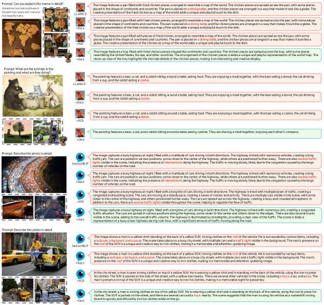
Figure 7: More qualitative results on LLaVA-Bench in the wild [35]. Our proposed Pensieve effectively reduces visual hallucinations for both MLLMs [34, 6]. Retrieved visual references are in the grey box. Hallucinatory content is marked in red.

0.C.3 More Results on MME

We present the results of all perception tasks on the MME [10] benchmark in Tab. 6. Our proposed Pensieve demonstrates an enhancement in the overall perception performance for both MLLMs [34, 6], surpassing other advanced decoding strategies [5, 22] to varying extents.

Table 6: Results on all perception tasks of the MME [10] benchmark. Our proposed Pensieve substantially improves the perception competencies for both MLLMs [34, 6].

Model	Decoding	Color $\uparrow$	Count $\uparrow$	Existence $\uparrow$	Position $\uparrow$	Posters $\uparrow$	Celebrity $\uparrow$	Scene $\uparrow$	Landmark $\uparrow$	Artwork $\uparrow$	OCR $\uparrow$	Total $\uparrow$
LLaVA-1.5	greedy	155.0	158.3	195.0	123.3	129.6	132.6	155.0	163.5	121.0	125.0	1458.9
	+DoLa	153.3	158.3	195.0	123.3	127.6	130.9	154.8	162.8	122.3	122.5	1450.7
	+VCD	148.3	158.3	190.0	126.7	136.7	147.4	148.8	166.0	122.5	130.0	1474.7
	+Ours	165.0	153.3	195.0	128.3	141.8	150.3	157.3	161.8	122.8	140.0	1515.5
InstructBLIP	greedy	120.0	60.0	185.0	50.0	142.9	81.8	160.0	160.0	92.0	65.0	1116.6
	+DoLa	120.0	60.0	185.0	50.0	142.9	80.9	160.0	160.0	92.2	65.0	1116.0
	+VCD	123.3	60.0	185.0	53.3	151.7	94.1	156.5	161.3	99.3	95.0	1179.5
	+Ours	153.3	78.3	180.0	58.3	140.5	71.2	163.8	158.3	94.3	95.0	1192.9

0.C.4 More Results on POPE

Detailed results for the three official splits of POPE [28] benchmark MSCOCO [30] dataset (the random, popular, and adversarial splits), are presented in Tab. 7. Pensieve demonstrates improvements in Accuracy and F1 score for LLaVA1.5 [34] across all splits, particularly outperforming DoLa [5] and VCD [22] in the adversarial split. On the other hand, Pensieve’s impact on InstructBLIP [6] shows slight variations across different splits, yet consistently outperforms VCD [22]. We notice that Pensieve enhances Precision for InstructBLIP [6] across all splits, indicating its capability to reduce false positives.

Table 7: Results on the POPE [28] benchmark MSCOCO [30] dataset. We report detailed results across the random, popular, and adversarial splits.

Setting	Model	Decoding	Acc. $\uparrow$	Prec.	Rec.	F1 $\uparrow$
Random	LLaVA-1.5	greedy	87.13	97.36	76.33	85.58
		+DoLa	86.93	97.43	75.87	85.31
		+VCD	88.63	92.08	84.53	88.15
		+Ours	87.53	96.76	77.66	86.17
	InstructBLIP	greedy	87.97	94.81	80.33	86.97
		+DoLa	88.00	94.67	80.53	87.03
		+VCD	87.07	93.92	79.27	85.97
		+Ours	87.83	94.93	79.93	86.79
Popular	LLaVA-1.5	greedy	85.90	94.39	76.33	84.41
		+DoLa	85.70	94.44	75.87	84.14
		+VCD	86.13	87.23	84.67	85.93
		+Ours	86.13	93.36	77.80	84.87
	InstructBLIP	greedy	84.97	88.54	80.33	84.24
		+DoLa	85.06	88.56	80.53	84.36
		+VCD	84.43	88.23	79.47	83.62
		+Ours	84.90	88.69	80.00	84.12
Adversarial	LLaVA-1.5	greedy	83.63	89.44	76.27	82.33
		+DoLa	83.50	89.60	75.80	82.12
		+VCD	82.00	80.23	84.93	82.51
		+Ours	83.73	88.33	77.73	82.70
	InstructBLIP	greedy	82.50	83.83	80.53	82.15
		+DoLa	82.56	83.81	80.73	82.24
		+VCD	81.77	83.53	79.13	81.27
		+Ours	82.63	84.25	80.27	82.21

0.C.5 More Ablations

0.C.5.1 Token Sampling.

Greedy search is employed as the baseline decoding strategy, i.e., always selecting the candidate with the highest confidence score. We further investigate the compatibility of Pensieve with various token sampling strategies, as outlined in Tab. 8. Greedy search achieves the highest performance as it avoids errors induced by token sampling. Our proposed Pensieve demonstrates versatility by effectively integrating with different sampling strategies, consistently enhancing image captioning performance and mitigating visual hallucination. For nucleus (Top-p) sampling, we set $p=0.9$. For Top-k sampling, we set $k=50$. We fix the random seeds in all experiments.

Table 8: Token sampling experiments on Whoops [2] benchmark. Pensieve enhances the performance for LLaVA-1.5 [34] across various baseline decoding strategies, including greedy search and different token sampling methods.

Method		B4 $\uparrow$	M $\uparrow$	C $\uparrow$	S $\uparrow$	FS% $\uparrow$
zeroshot
LLaVA-1.5 [34] Vicuna-7B	greedy	19.7	25.6	67.9	17.3	67.9
	+Ours	20.0	26.3	75.5	17.8	68.3
	sample	6.9	19.0	31.4	12.0	57.8
	+Ours	8.8	20.3	40.6	13.7	61.9
	nucleus	9.6	20.5	39.4	13.3	62.4
	+Ours	10.7	21.8	46.8	14.0	65.4
	Top-k	8.0	19.3	33.6	12.3	59.1
	+Ours	8.8	20.3	40.6	13.7	62.4

0.C.5.2 Effect of Hyper-parameters.

In our paradigm, decreasing $\beta_{d}$ and $\beta_{NN}$, or increasing $\alpha_{\tau}$ diminishes the influence of Pensieve, preserving the original confidence score distribution predicted without visual references. We investigate the impact of $\beta_{d}$ and $\beta_{NN}$, while keeping $k=2$, $\alpha_{\tau}=1.0$ and the diffusion step to 900 on the $LLaVA^{W}$ Detail Description split. We calculate the average FaithScore [16] across all samples and provide a qualitative example (see Fig. 8).

The default hyper-parameter setting (see Sec. 0.C.1.2) serves as an effective baseline for LLaVA-1.5 [34], validating the efficacy of our proposed Pensieve. Additionally, we observe that the performance can be sensitive to these hyper-parameters; a change of 0.05 can enhance overall performance but may induce extra visual hallucinations in the provided example (e.g., cups and the strawberries outside the container).

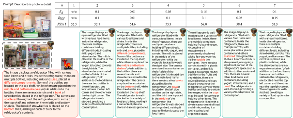
Figure 8: We study the effect of hyper-parameters $\beta_{d}$ and $\beta_{NN}$ in our paradigm on the Detail Description split of $LLaVA^{W}$ [35]. We compare the averaged FaithScore [16] ($FS\%$) and provide an example. Our default hyper-parameter setting serves as a baseline to validate the efficacy of Pensieve. If $\beta_{d}$ and $\beta_{NN}$ are not sufficiently large, Pensieve may fail to correct visual hallucinations in this example.

Appendix 0.D More Examples to Support our Premise

We provide more examples in Figs. 9, 10, 11, 12, 13, 14 and 15 to support our premise that images with similar semantics and appearance are likely to induce analogous visual hallucinations. For instance, $\_ju$, $\_orange$, $\_bow$, $\_cup$, $\_bottom$, $\_middle$ in Fig. 9, $\_du$, $\_fish$ in Fig. 10 (the references images show swans), $\_c$, $\_l$ (first token for lollipop), $\_apple$ in Fig. 11, the article $\_a$ and $\_an$ (may deviate subsequent content from flames), and $\_h$ (first token for hose) in Fig. 12, $\_woman$ in Fig. 13, $\_kn$ (first token for knight), $\_queen$, and $\_piece$ in Fig. 14.

Moreover, MLLMs are not utterly blind when they generate hallucinatory tokens in these examples, as they do recognize the accurate candidates, such as $\_y$ (first token for yogurt), $\_st$ (first token for strawberry), $\_stored$, $\_left$ in Fig. 9, $\_rub$, $\_yellow$ in Fig. 10, $\_hot$, $\_pe$ in Fig. 11, $\_fl$, $\_fire$ in Fig. 12, $\_liberty$ in Fig. 13, $\_un$ (first token for unicorn) in Fig. 14, $\_sad$ in Fig. 15.

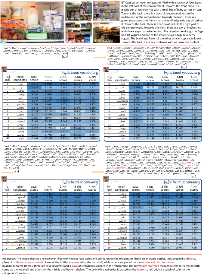
Figure 9: More qualitative evidence to support our hypothesis. This sample is from the LLaVA Bench in the wild [35] benchmark. Hallucinatory content is marked red.

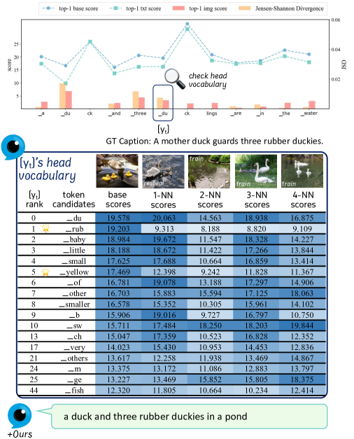
Figure 10: More qualitative evidence to support our hypothesis. This example is from the Whoops [2] benchmark.

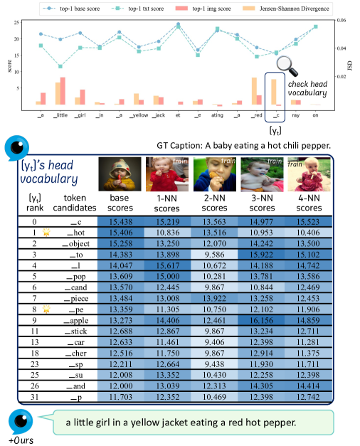
Figure 11: More qualitative evidence to support our hypothesis. This example is from the Whoops [2] benchmark.

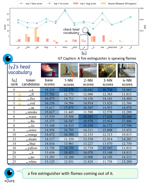
Figure 12: More qualitative evidence to support our hypothesis. This example is from the Whoops [2] benchmark.

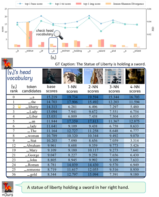
Figure 13: More qualitative evidence to support our hypothesis. This example is from the Whoops [2] benchmark.

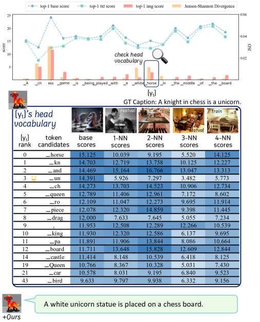
Figure 14: More qualitative evidence to support our hypothesis. This example is from the Whoops [2] benchmark.

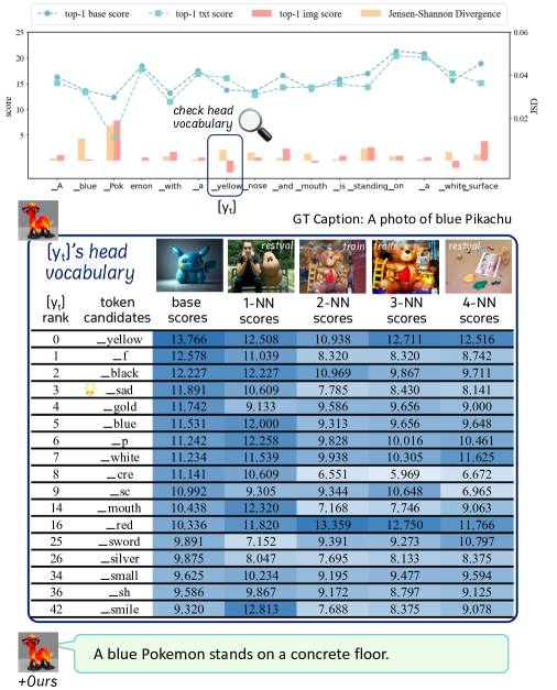
Figure 15: More qualitative evidence to support our hypothesis. This example is from the Whoops [2] benchmark.

References

- [1] Anderson, P., Fernando, B., Johnson, M., Gould, S.: Spice: Semantic propositional image caption evaluation. In: Computer Vision–ECCV 2016: 14th European Conference, Amsterdam, The Netherlands, October 11-14, 2016, Proceedings, Part V 14. pp. 382–398. Springer (2016)
- [2] Bitton-Guetta, N., Bitton, Y., Hessel, J., Schmidt, L., Elovici, Y., Stanovsky, G., Schwartz, R.: Breaking common sense: Whoops! a vision-and-language benchmark of synthetic and compositional images. In: Proceedings of the IEEE/CVF International Conference on Computer Vision. pp. 2616–2627 (2023)
- [3] Chen, K., Zhang, Z., Zeng, W., Zhang, R., Zhu, F., Zhao, R.: Shikra: Unleashing multimodal llm’s referential dialogue magic. arXiv preprint arXiv:2306.15195 (2023)
- [4] Chen, Z., Zhu, Y., Zhan, Y., Li, Z., Zhao, C., Wang, J., Tang, M.: Mitigating hallucination in visual language models with visual supervision. arXiv preprint arXiv:2311.16479 (2023)
- [5] Chuang, Y.S., Xie, Y., Luo, H., Kim, Y., Glass, J., He, P.: Dola: Decoding by contrasting layers improves factuality in large language models. arXiv preprint arXiv:2309.03883 (2023)
- [6] Dai, W., Li, J., Li, D., Tiong, A.M.H., Zhao, J., Wang, W., Li, B., Fung, P., Hoi, S.: Instructblip: Towards general-purpose vision-language models with instruction tuning (2023)
- [7] Denkowski, M., Lavie, A.: Meteor universal: Language specific translation evaluation for any target language. In: Proceedings of the ninth workshop on statistical machine translation. pp. 376–380 (2014)
- [8] Dosovitskiy, A., Beyer, L., Kolesnikov, A., Weissenborn, D., Zhai, X., Unterthiner, T., Dehghani, M., Minderer, M., Heigold, G., Gelly, S., et al.: An image is worth 16x16 words: Transformers for image recognition at scale. arXiv preprint arXiv:2010.11929 (2020)
- [9] Douze, M., Guzhva, A., Deng, C., Johnson, J., Szilvasy, G., Mazaré, P.E., Lomeli, M., Hosseini, L., Jégou, H.: The faiss library (2024)
- [10] Fu, C., Chen, P., Shen, Y., Qin, Y., Zhang, M., Lin, X., Yang, J., Zheng, X., Li, K., Sun, X., et al.: Mme: A comprehensive evaluation benchmark for multimodal large language models. arXiv preprint arXiv:2306.13394 (2023)
- [11] Gera, A., Friedman, R., Arviv, O., Gunasekara, C., Sznajder, B., Slonim, N., Shnarch, E.: The benefits of bad advice: Autocontrastive decoding across model layers. arXiv preprint arXiv:2305.01628 (2023)
- [12] Hessel, J., Holtzman, A., Forbes, M., Bras, R.L., Choi, Y.: Clipscore: A reference-free evaluation metric for image captioning. arXiv preprint arXiv:2104.08718 (2021)
- [13] Ho, J., Jain, A., Abbeel, P.: Denoising diffusion probabilistic models. Advances in neural information processing systems 33, 6840–6851 (2020)
- [14] Huang, Q., Dong, X., Zhang, P., Wang, B., He, C., Wang, J., Lin, D., Zhang, W., Yu, N.: Opera: Alleviating hallucination in multi-modal large language models via over-trust penalty and retrospection-allocation. arXiv preprint arXiv:2311.17911 (2023)
- [15] Jiang, C., Xu, H., Dong, M., Chen, J., Ye, W., Yan, M., Ye, Q., Zhang, J., Huang, F., Zhang, S.: Hallucination augmented contrastive learning for multimodal large language model. arXiv preprint arXiv:2312.06968 (2023)
- [16] Jing, L., Li, R., Chen, Y., Jia, M., Du, X.: Faithscore: Evaluating hallucinations in large vision-language models. arXiv preprint arXiv:2311.01477 (2023)
- [17] Karpathy, A., Fei-Fei, L.: Deep visual-semantic alignments for generating image descriptions. In: Proceedings of the IEEE conference on computer vision and pattern recognition. pp. 3128–3137 (2015)
- [18] Kim, T., Kim, J., Lee, G., Yun, S.Y.: Distort, distract, decode: Instruction-tuned model can refine its response from noisy instructions. arXiv preprint arXiv:2311.00233 (2023)
- [19] Krishna, R., Zhu, Y., Groth, O., Johnson, J., Hata, K., Kravitz, J., Chen, S., Kalantidis, Y., Li, L.J., Shamma, D.A., et al.: Visual genome: Connecting language and vision using crowdsourced dense image annotations. International journal of computer vision 123, 32–73 (2017)
- [20] Lee, N., Ping, W., Xu, P., Patwary, M., Fung, P.N., Shoeybi, M., Catanzaro, B.: Factuality enhanced language models for open-ended text generation. Advances in Neural Information Processing Systems 35, 34586–34599 (2022)
- [21] Lee, S., Park, S.H., Jo, Y., Seo, M.: Volcano: mitigating multimodal hallucination through self-feedback guided revision. arXiv preprint arXiv:2311.07362 (2023)
- [22] Leng, S., Zhang, H., Chen, G., Li, X., Lu, S., Miao, C., Bing, L.: Mitigating object hallucinations in large vision-language models through visual contrastive decoding. arXiv preprint arXiv:2311.16922 (2023)
- [23] Li, J., Vo, D.M., Sugimoto, A., Nakayama, H.: Evcap: Retrieval-augmented image captioning with external visual-name memory for open-world comprehension. arXiv preprint arXiv:2311.15879 (2023)
- [24] Li, J., Li, D., Savarese, S., Hoi, S.: Blip-2: Bootstrapping language-image pre-training with frozen image encoders and large language models. arXiv preprint arXiv:2301.12597 (2023)
- [25] Li, J., Li, D., Xiong, C., Hoi, S.: Blip: Bootstrapping language-image pre-training for unified vision-language understanding and generation. In: International Conference on Machine Learning. pp. 12888–12900. PMLR (2022)
- [26] Li, J., Chen, J., Ren, R., Cheng, X., Zhao, W.X., Nie, J.Y., Wen, J.R.: The dawn after the dark: An empirical study on factuality hallucination in large language models. arXiv preprint arXiv:2401.03205 (2024)
- [27] Li, X.L., Holtzman, A., Fried, D., Liang, P., Eisner, J., Hashimoto, T., Zettlemoyer, L., Lewis, M.: Contrastive decoding: Open-ended text generation as optimization. arXiv preprint arXiv:2210.15097 (2022)
- [28] Li, Y., Du, Y., Zhou, K., Wang, J., Zhao, W.X., Wen, J.R.: Evaluating object hallucination in large vision-language models. arXiv preprint arXiv:2305.10355 (2023)
- [29] Lin, B.Y., Ravichander, A., Lu, X., Dziri, N., Sclar, M., Chandu, K., Bhagavatula, C., Choi, Y.: The unlocking spell on base llms: Rethinking alignment via in-context learning. arXiv preprint arXiv:2312.01552 (2023)
- [30] Lin, T.Y., Maire, M., Belongie, S., Hays, J., Perona, P., Ramanan, D., Dollár, P., Zitnick, C.L.: Microsoft coco: Common objects in context. In: Computer Vision–ECCV 2014: 13th European Conference, Zurich, Switzerland, September 6-12, 2014, Proceedings, Part V 13. pp. 740–755. Springer (2014)
- [31] Lin, Z., Liu, C., Zhang, R., Gao, P., Qiu, L., Xiao, H., Qiu, H., Lin, C., Shao, W., Chen, K., et al.: Sphinx: The joint mixing of weights, tasks, and visual embeddings for multi-modal large language models. arXiv preprint arXiv:2311.07575 (2023)
- [32] Liu, F., Lin, K., Li, L., Wang, J., Yacoob, Y., Wang, L.: Mitigating hallucination in large multi-modal models via robust instruction tuning. arXiv preprint arXiv:2306.14565 1(2), 9 (2023)
- [33] Liu, H., Xue, W., Chen, Y., Chen, D., Zhao, X., Wang, K., Hou, L., Li, R., Peng, W.: A survey on hallucination in large vision-language models. arXiv preprint arXiv:2402.00253 (2024)
- [34] Liu, H., Li, C., Li, Y., Lee, Y.J.: Improved baselines with visual instruction tuning (2023)
- [35] Liu, H., Li, C., Wu, Q., Lee, Y.J.: Visual instruction tuning. Advances in neural information processing systems 36 (2024)
- [36] Liu, Y., Duan, H., Zhang, Y., Li, B., Zhang, S., Zhao, W., Yuan, Y., Wang, J., He, C., Liu, Z., et al.: Mmbench: Is your multi-modal model an all-around player? arXiv preprint arXiv:2307.06281 (2023)
- [37] Oquab, M., Darcet, T., Moutakanni, T., Vo, H., Szafraniec, M., Khalidov, V., Fernandez, P., Haziza, D., Massa, F., El-Nouby, A., et al.: Dinov2: Learning robust visual features without supervision. arXiv preprint arXiv:2304.07193 (2023)
- [38] Papineni, K., Roukos, S., Ward, T., Zhu, W.J.: Bleu: a method for automatic evaluation of machine translation. In: Proceedings of the 40th annual meeting of the Association for Computational Linguistics. pp. 311–318 (2002)
- [39] Radford, A., Kim, J.W., Hallacy, C., Ramesh, A., Goh, G., Agarwal, S., Sastry, G., Askell, A., Mishkin, P., Clark, J., et al.: Learning transferable visual models from natural language supervision. In: International conference on machine learning. pp. 8748–8763. PMLR (2021)
- [40] Rasheed, H., Maaz, M., Shaji, S., Shaker, A., Khan, S., Cholakkal, H., Anwer, R.M., Xing, E., Yang, M.H., Khan, F.S.: Glamm: Pixel grounding large multimodal model. arXiv preprint arXiv:2311.03356 (2023)
- [41] Rohrbach, A., Hendricks, L.A., Burns, K., Darrell, T., Saenko, K.: Object hallucination in image captioning. arXiv preprint arXiv:1809.02156 (2018)
- [42] Shi, W., Han, X., Lewis, M., Tsvetkov, Y., Zettlemoyer, L., Yih, S.W.t.: Trusting your evidence: Hallucinate less with context-aware decoding. arXiv preprint arXiv:2305.14739 (2023)
- [43] Sun, Z., Shen, S., Cao, S., Liu, H., Li, C., Shen, Y., Gan, C., Gui, L.Y., Wang, Y.X., Yang, Y., et al.: Aligning large multimodal models with factually augmented rlhf. arXiv preprint arXiv:2309.14525 (2023)
- [44] Tong, S., Liu, Z., Zhai, Y., Ma, Y., LeCun, Y., Xie, S.: Eyes wide shut? exploring the visual shortcomings of multimodal llms. arXiv preprint arXiv:2401.06209 (2024)
- [45] Touvron, H., Martin, L., Stone, K., Albert, P., Almahairi, A., Babaei, Y., Bashlykov, N., Batra, S., Bhargava, P., Bhosale, S., et al.: Llama 2: Open foundation and fine-tuned chat models. arXiv preprint arXiv:2307.09288 (2023)
- [46] Vaswani, A., Shazeer, N., Parmar, N., Uszkoreit, J., Jones, L., Gomez, A.N., Kaiser, Ł., Polosukhin, I.: Attention is all you need. Advances in neural information processing systems 30 (2017)
- [47] Vedantam, R., Lawrence Zitnick, C., Parikh, D.: Cider: Consensus-based image description evaluation. In: Proceedings of the IEEE conference on computer vision and pattern recognition. pp. 4566–4575 (2015)
- [48] Villa, A., Alcazar, J.C.L., Soto, A., Ghanem, B.: Behind the magic, merlim: Multi-modal evaluation benchmark for large image-language models. arXiv preprint arXiv:2312.02219 (2023)
- [49] Wang, J., Wang, Y., Xu, G., Zhang, J., Gu, Y., Jia, H., Yan, M., Zhang, J., Sang, J.: An llm-free multi-dimensional benchmark for mllms hallucination evaluation. arXiv preprint arXiv:2311.07397 (2023)
- [50] Wang, J., Zhou, Y., Xu, G., Shi, P., Zhao, C., Xu, H., Ye, Q., Yan, M., Zhang, J., Zhu, J., et al.: Evaluation and analysis of hallucination in large vision-language models. arXiv preprint arXiv:2308.15126 (2023)
- [51] Wang, P., Yang, A., Men, R., Lin, J., Bai, S., Li, Z., Ma, J., Zhou, C., Zhou, J., Yang, H.: Ofa: Unifying architectures, tasks, and modalities through a simple sequence-to-sequence learning framework. CoRR abs/2202.03052 (2022)
- [52] Wang, X., Zhou, Y., Liu, X., Lu, H., Xu, Y., He, F., Yoon, J., Lu, T., Bertasius, G., Bansal, M., et al.: Mementos: A comprehensive benchmark for multimodal large language model reasoning over image sequences. arXiv preprint arXiv:2401.10529 (2024)
- [53] Wu, P., Xie, S.: V*: Guided visual search as a core mechanism in multimodal llms. arXiv preprint arXiv:2312.14135 (2023)
- [54] Xie, N., Lai, F., Doran, D., Kadav, A.: Visual entailment: A novel task for fine-grained image understanding. arXiv preprint arXiv:1901.06706 (2019)
- [55] Xu, Z., Feng, C., Shao, R., Ashby, T., Shen, Y., Jin, D., Cheng, Y., Wang, Q., Huang, L.: Vision-flan: Scaling human-labeled tasks in visual instruction tuning. arXiv preprint arXiv:2402.11690 (2024)
- [56] Yin, S., Fu, C., Zhao, S., Xu, T., Wang, H., Sui, D., Shen, Y., Li, K., Sun, X., Chen, E.: Woodpecker: Hallucination correction for multimodal large language models. arXiv preprint arXiv:2310.16045 (2023)
- [57] You, H., Zhang, H., Gan, Z., Du, X., Zhang, B., Wang, Z., Cao, L., Chang, S.F., Yang, Y.: Ferret: Refer and ground anything anywhere at any granularity. arXiv preprint arXiv:2310.07704 (2023)
- [58] Yuan, Y., Li, W., Liu, J., Tang, D., Luo, X., Qin, C., Zhang, L., Zhu, J.: Osprey: Pixel understanding with visual instruction tuning. arXiv preprint arXiv:2312.10032 (2023)
- [59] Zhai, B., Yang, S., Zhao, X., Xu, C., Shen, S., Zhao, D., Keutzer, K., Li, M., Yan, T., Fan, X.: Halle-switch: Rethinking and controlling object existence hallucinations in large vision language models for detailed caption. arXiv preprint arXiv:2310.01779 (2023)
- [60] Zhang, M., Press, O., Merrill, W., Liu, A., Smith, N.A.: How language model hallucinations can snowball. arXiv preprint arXiv:2305.13534 (2023)
- [61] Zhang, S., Sun, P., Chen, S., Xiao, M., Shao, W., Zhang, W., Chen, K., Luo, P.: Gpt4roi: Instruction tuning large language model on region-of-interest. arXiv preprint arXiv:2307.03601 (2023)
- [62] Zhang, Y., Cui, L., Bi, W., Shi, S.: Alleviating hallucinations of large language models through induced hallucinations. arXiv preprint arXiv:2312.15710 (2023)
- [63] Zhao, L., Deng, Y., Zhang, W., Gu, Q.: Mitigating object hallucination in large vision-language models via classifier-free guidance. arXiv preprint arXiv:2402.08680 (2024)
- [64] Zhao, Z., Wallace, E., Feng, S., Klein, D., Singh, S.: Calibrate before use: Improving few-shot performance of language models. In: International Conference on Machine Learning. pp. 12697–12706. PMLR (2021)
- [65] Zheng, L., Chiang, W.L., Sheng, Y., Zhuang, S., Wu, Z., Zhuang, Y., Lin, Z., Li, Z., Li, D., Xing, E.P., Zhang, H., Gonzalez, J.E., Stoica, I.: Judging llm-as-a-judge with mt-bench and chatbot arena (2023)
- [66] Zhou, Y., Cui, C., Yoon, J., Zhang, L., Deng, Z., Finn, C., Bansal, M., Yao, H.: Analyzing and mitigating object hallucination in large vision-language models. arXiv preprint arXiv:2310.00754 (2023)
- [67] Zhu, D., Chen, J., Shen, X., Li, X., Elhoseiny, M.: Minigpt-4: Enhancing vision-language understanding with advanced large language models. arXiv preprint arXiv:2304.10592 (2023)