Space-time quasicrystals in Bose-Einstein condensates

Abstract

An autoresonant approach for exciting space-time quasicrystals in Bose-Einstein condensates is proposed by employing two-component chirped frequency parametric driving or modulation of the interaction strength within Gross-Pitaevskii equation. A weakly nonlinear theory of the process is developed using Whitham’s averaged variational principle yielding reduction to a two-degrees-of-freedom dynamical system in action-angle variables. Additionally, the theory also delineates permissible driving parameters and establishes thresholds on the driving amplitudes required for autoresonant excitation.

I Introduction

Quasicrystals in materials are structures ordered in space, but not exactly periodic Shechtman ; Levine ; Senechal . By analogy, time or space-time quasicrystals are ordered systems in space-time, but not exactly periodic in space and/or time. By now, these systems have been studied in periodically driven magnon condensates Autti ; Kreil and ultracold atoms Giergiel ; Cosme , where temporal symmetry was destroyed due to subharmonic response. In this study, we explore a different path to space-time quasicrystals. It is well known that a number of so-called integrable nonlinear partial differential equations (PDE’s) have multiphase solutions Scott of the form $f(\theta_{1},\theta_{2},...,\theta_{N};\lambda_{1},\lambda_{2},...,\lambda_{N})$, where $N$ phase variables $\theta_{i}=k_{i}x-\omega_{i}t$ have wave numbers $k_{i}$ which are multiples of some $k_{0}$ (the solution is spatially periodic), $\lambda_{i}$ are constants, while frequencies $\omega_{i}$ are functions of $k_{i}$ and $\lambda_{i}$. By choosing some set of $\lambda_{i}$, one can make some or all of these frequencies incommensurate, forming an ideal space-time quasicrystalline structure, which is periodic in space and aperiodic in time, still having a complex long range time ordering. Examples of such PDEs are the Korteweg-de-Vries (KdV), sine-Gordon (SG), and nonlinear Schrodinger (NLS) equations, which find multiple application in physics Scott . However, why these ideal space-time quasicrystals are not yet realized in experiments? The answer lies in complexity, as their analysis typically requires advanced mathematical methods, such as the inverse scattering transform (IST) Novikov , while experimental realization depends on forming complicated space-time dependent initial conditions, which is an unrealistic task.

In this work, we suggest a different approach to realizing space-time quasicrystals based on autoresonance LazarWiki . Autoresonance is an important nonlinear phenomenon, where a system phase-locks to a chirped frequency driving perturbation and remains phase-locked continuously for an extended period of time, despite variations of the driving frequency. As the driving frequency varies in time, so does the frequency of the excited solution, leading to formation of a stable highly nonlinear state. We will focus on autoresonant formation and control of two-phase excitations of the Gross-Pitaevskii (GP) equation describing Bose-Einstein condensates (BECs). The excitation proceeds from trivial initial conditions and uses a combination of two independent small amplitude wave-like driving perturbations. In contrast to existing applications using large amplitude pulsed drives or optical crystalline structures for containing BEC’s, we can remove the driving perturbation after some time, remaining with a free, slightly perturbed, but stable nonlinear two-phase GP solution. These excited quasicrystalline structures are controlled by two independently chirped driving frequencies, thus exploring a continuous range of parameters $\lambda_{i}$, i.e., a continuous set of space-time quasicrystals. The autoresonance approach has been used previously in excitation of multi-phase waves in different applications with the theory based on the IST method Lazar2003 ; Lazar2005 ; Lazar2009 . Here we will apply a simpler analysis of the process of capture into a double autoresonance in the system using two chirped frequency drives, similar to recent studies on the formation of two-phase waves in plasmas Munirov1 ; Munirov2 .

Our presentation will be as follows. In the next section, we illustrate the formation of space-time quasicrystals in BECs through numerical simulations. Section III presents the quasi-linear theory of formation of GP quasicrystals using Whitham’s averaged variational approach Whitham . Section IV addresses the problem of the allowed parameter space for autoresonant excitations and with the associated threshold phenomenon on the driving amplitudes. Finally, Sec. V presents our conclusions.

II Quasicrystals in a BEC via simulations

The basic model for studying nonlinear dynamics of BECs is GP equation Dalfovo ,written in dimensionless form

$$i\varphi_{t}+\varphi_{xx}-\mathbf{U}(x,t)\varphi+g(x,t)|\varphi|^{2}\varphi=0.$$ (1)

Here, time is measured in units of the inverse transverse trapping frequency $\omega_{\bot}^{-1}$, while space and density are measure in units of $l_{\bot}=[\hbar/(2m\omega_{\bot})]^{1/2}$ and $m\omega_{\bot}/2\pi\hbar|a_{0}|$, respectively, where $m$ represents the atomic mass. In Eq. (1), $g=2a(x,t)/|a_{0}|$ is the normalized, space-time modulated interaction strength, where $a$ represents the $s$-wave scattering length of interacting particles in the BEC. For condensates with repulsive interactions of particles $a<0$ and for attractive interactions $a>0$. $\mathbf{U}(x,t)$ denotes the longitudinal potential. We will assume that our system is perturbed by a combination of independent, small amplitude waves

$$f=\varepsilon_{1}\cos[k_{1}x-\psi_{1}(t)]-\varepsilon_{2}\cos[k_{2}x-\psi_{2}(t)],$$ (2)

where $\psi_{i}(t)=\int\omega_{di}(t)dt$ and $\omega_{di}(t)=\omega_{0i}-\alpha_{i}t$ are slowly chirped driving frequencies. We consider two driving options. The first is a parametric-type driving $\mathbf{U}(x,t)=f$, $|f|\ll 1$, while the interaction strength is not perturbed, i.e., $g=2\sigma$ and $\sigma=\pm 1$. The second driving scenario is a modulation of the interaction strength by external magnetic field,for example, near Feshbach resonance Yamazaki . In this case, we assume $\mathbf{U}=0$,

$$g(x,t)=2\sigma(1+f),$$ (3)

and again $|f|\ll 1$. For both driving options we can rewrite Eq. (1) as a weakly perturbed NLS equation

$$i\varphi_{t}+\varphi_{xx}+2\sigma|\varphi|^{2}\varphi=F\varphi,$$ (4)

where $F\$is either $-f$ or $-2\sigma|\varphi|^{2}f$. In computer simulations below, we will use the parametric driving, assume periodic boundary conditions $\varphi(x,t)=\varphi(x+l,t)$, thus $k_{1,2}$ are multiples of $k_{0}=2\pi/l$. Nevertheless, in Secs. III and IV, we will discuss both driving options. It should be mentioned that periodic boundary conditions are usually assumed in numerical simulations of an infinite domain for a spatially periodic driving as well as in 1D modeling along the torus-like BEC (ring-trap geometry) Schloss ; Zhu . A special case when the driving (3) is a standing wave, i.e. $\varepsilon_{1}=\varepsilon_{2}$, $\psi_{1}=\psi_{2}$, and $k_{1}=-k_{2}$ was studied recently solitons , so the present investigation is a generalization to two independent driving components.

In the periodic case, the unperturbed ground state of a BEC is a spatially homogeneous solution of Eq. (4)

$$\varphi(x,t)=U_{0}e^{2i\sigma U_{0}^{2}t}$$ (5)

with constant amplitude $|\varphi|=U_{0}$. The frequency of a perturbation of the homogeneous state is Leggett

$$\omega_{0}=k\sqrt{k^{2}-4\sigma U_{0}^{2}}.$$ (6)

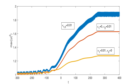
Figure 1: Maximum of $|\varphi|^{2}$ over x versus time. The upper line corresponds to nonzero driving amplitudes $\epsilon_{1,2}$. The middle and the lower lines describe the cases when either $\epsilon_{1}=0$ or $\epsilon_{2}=0$, respectively. In all cases the drives are switched off at $t=250$

Condensates with repulsive interaction of particles, when $\sigma=-1$, are stable. In this case, frequency (6) is known as the Bogolubov frequency. Dark solitons are typical structures in these condensates. In the opposite case ($\sigma=1$), bright solitons exists. In this case $\omega_{0}$ can be imaginary, leading to modulational instability. This instability is well-known in plasma physics and nonlinear optics Zakharov ; Agrawal . If a condensate has a length $l$, then the wave number of the main mode is $k_{0}=2\pi/l$ and the stability condition restricts the density of the condensate to $U_{0}^{2}<\pi^{2}/l^{2}$. If the condensate has a cigar-like shape with the transverse dimension $l_{\bot}$, then, in physical variables, the stability condition can be written as a restriction on the number of particles, $n<(l_{\bot}/l)(l_{\bot}/|a_{0}|).$

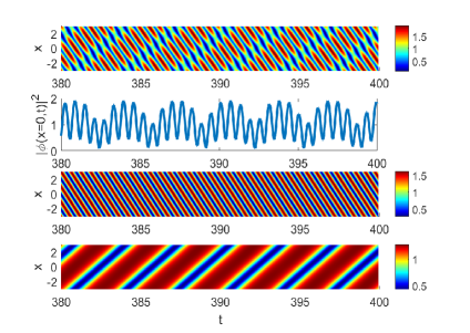
Figure 2: Two- and one-phase autoresonant excitations in simulations. The upper panel shows the color map of a two-phase solution $|\varphi|^{2}$ in space-time for driving parameters $\varepsilon_{1,2}=0.01$, $k_{1,2}=1,-3$, chirp rates $\alpha_{1,2}=0.0012,0.0024$. The second panel from the top shows $|\varphi|^{2}$ versus time at $x=0$, illustrating 1:5 quasi-periodicity of the solution. The lowest two panels show color maps of autoresonant single-phase excitations $|\varphi|^{2}$ for the same parameters and initial conditions as in the upper panel, but when only one of the diving components is applied.

We proceed to numerical simulations of autoresonant formation of a space-time GP quasicrystal by focusing on the case of $\sigma=-1$ and starting in the ground state (5) with $U_{0}=1$. The driving parameters are $\varepsilon_{1,2}=0.01$, $k_{1,2}=1,-3$, chirp rates $\alpha_{1,2}=0.0012,0.0024$, and $\omega_{0i}$ are given by Eq. (6) for each $k_{i}$. The simulation begins at $t_{0}=-300$ and both components of the drive pass the corresponding Bogolubov resonances at $t=0.$ Furthermore, we switch off the drives at $t=t_{s}=250$. The corresponding time dependence of the maximum (over $x$) $|\varphi|^{2}$ is shown in Fig. 1 by the upper blue line. One can observe that the excitation amplitude increases continuously until the drive is turned off, and the maximal amplitude remains nearly stationary afterwards. We also show the excited quasicrystalline structure in the time interval $380<t<400$ (after the driving is switched off) using a colormap in the upper panel of Fig. 2. Furthermore, the ratio of the two driving frequencies at $t=t_{s}$ in this example is approximately $1:5$. The second panel from the top in Fig. 2 shows $|\varphi|^{2}$ versus time in the same example at $x=0$. One can see the short and long driving periods in the panel illustrating $1:5$ quasi-periodicity and the two-phase locking with the drives.

To further illustrate the characteristics of autoresonant excitation in the system, we show, by the lower two lines in Fig. 1, the cases when only one of the two drives is present in the same example and illustrate the colormaps of the associated excitations in the lowest two panels in Fig. 2. A single-phase parametric autoresonant excitation in this system was analyzed in Ref. Lazar2022 . In this case, one forms a growing amplitude nonlinear wave traveling with the phase velocity $\omega_{di}/k_{i}$ of the corresponding drive. The directions of these propagation velocities are clearly seen in Fig. 2. We observe the same two characteristic directions in the upper panel in Fig. 2 corresponding to the two-phase autoresonant excitation, illustrating again the continuing phase locking with the two driving components.

One of the most important issues associated with the autoresonance is the threshold on the driving amplitudes for the continuing phase locking in the system. Figures 1 and 2 show that the two-phase autoresonant excitation (where both drives are present) is very different from that with a single drive. This means that the driving amplitudes must be sufficiently large to obtain a two-phase quasicrystalline structure, leading to the problem of thresholds for the transition to autoresonance. We illustrate this sudden transition in Fig. 3, showing the maximal $|\varphi|^{2}$ versus time in three cases with the same parameters as in Fig. 1, but $\varepsilon_{2}=0.006,0.005$, and $0.004$, while keeping $\epsilon_{1}=0.01$. One observes a sharp transition when passing from $\epsilon_{2}=0.005$ to $0.004$. The color maps of $|\varphi|^{2}$ in space-time in these three cases are shown in Fig. 4. One can see that the quasicrystalilne structure in the upper two panels in the Figure is similar to that shown in the upper panel in Fig. 2, but the structure changes significantly as one passes to $\epsilon_{2}=0.004$. The lowest panel in Fig. 4 has smaller amplitude and is closer to the lowest panel in Fig. 2, corresponding to the single phase excitation. We interpret this transition as the loss of the phase locking when $\epsilon_{2}$ is below some threshold value between $\epsilon_{2}=0.004$ and $0.005$.

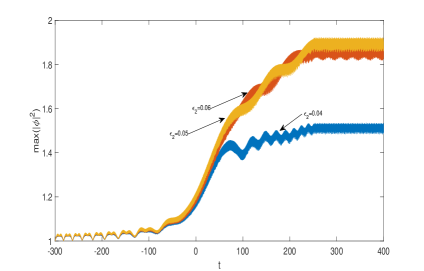
Figure 3: The passage through threshold. The figure shows the color maps of $max(|\varphi|^{2})$ over $x$ versus time for three values of $\epsilon_{2}=0.006,0.005,0.004$. In all cases $\epsilon_{1}=0.01$, $\alpha_{1}=0.0012$ and $\alpha_{2}=0.0024$.

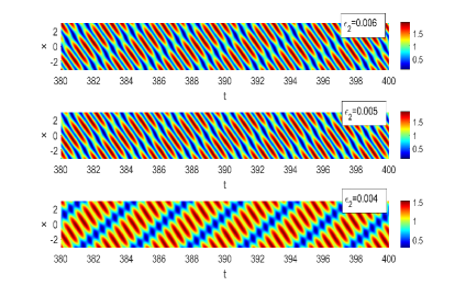
Figure 4: The passage through threshold. The colormaps of $|\varphi|^{2}$ over $x$ in space-time in three examples shown in Fig. 3.

As in all single phase autoresonant interactions, the double autoresonant phase locking in the driven GP system starts in the initial excitation stage, as the two drives simultaneously pass through the linear (Bogolubov) frequencies in the problem. We also find that the autoresonant phase locking is a weakly nonlinear phenomenon. Therefore, the next section is devoted to the quasi-linear theory of two-phase GP autoresonance.

III Weakly nonlinear theory

In developing the weakly nonlinear theory of autoresonant two-phase solutions of the GP equation, we will focus primarily on the parametric-type driving scenario. The case of driving by modulation of the interaction strength is obtained similarly and will be briefly discussed at the end of this Section. Therefore, we proceed from Eq. (4) for the ponderomotive case

$$i\varphi_{t}+\varphi_{xx}+2\sigma\left|\varphi\right|^{2}\varphi=-\varphi(\varepsilon_{1}\cos\theta_{d1}-\varepsilon_{2}\cos\theta_{d2}),$$ (7)

where $\theta_{di}=k_{i}x-\psi_{di}(t)$ and seek solution of form $\varphi=U\exp(iV)$ governed by the following set of real equations

$$U_{t}+V_{xx}U+2V_{x}U_{x}=0,$$ (8)

$$V_{t}U-U_{xx}+V_{x}^{2}U-2\sigma U^{3}=U(\varepsilon_{1}\cos\theta_{d1}-\varepsilon_{2}\cos\theta_{d2}).$$ (9)

The Lagrangian density for this problem is

$$L= \frac{1}{2}\left[U_{x}^{2}+U^{2}(V_{x}^{2}+V_{t})\right]-\frac{\sigma}{2}U^{4}$$ (10)

$$-\frac{U^{2}}{2}(\varepsilon_{1}\cos\theta_{d1}-\varepsilon_{2}\cos\theta_{d2}).$$

This Lagrangian representation suggests using Whitham’s averaged variational approach Whitham to analyze our problem. The first step in this direction is to assume constant frequency drives, $\psi_{di}=\omega_{di}t$, and seek phase-locked solutions of the linearized problem of form

$$U = U_{0}+U_{1}\cos\theta_{d1}-U_{2}\cos\theta_{d2},$$ (11)

$$V = 2\sigma U_{0}^{2}t+V_{1}\sin\theta_{d1}+V_{2}\sin\theta_{d2},$$ (12)

[Note that our unperturbed solution is $\varphi_{0}=U_{0}\exp(2i\sigma U_{0}^{2}t)$]. Then, by linearization, and neglecting products of linear amplitudes $U_{i}$ and $\varepsilon_{i}$, Eqs (8) and (9) become

$$\omega_{di}U_{i}-k_{i}^{2}U_{0}V_{i}=0,$$ (13)

$$-\omega_{di}V_{i}U_{0}+(k_{i}^{2}-4\sigma U_{0}^{2})U_{i}=\varepsilon_{i}U_{0},$$ (14)

yielding solutions

$$V_{i} = \frac{\varepsilon\omega_{di}}{(\omega_{0i}^{2}-\omega_{di}^{2})},$$ (15)

$$U_{i} = \frac{k_{i}^{2}U_{0}}{\omega_{di}}V_{i},$$ (16)

where the linear resonance frequencies

$$\omega_{0i}=\left|k_{i}\right|\sqrt{k_{i}^{2}-4\sigma U_{0}^{2}}.$$ (17)

Now, we proceed to chirped-driven problem, where $\psi_{i}=\int\omega_{di}(t)dt$ and extend Eqs. (11) and (12) to next nonlinear order

$$U =U_{0}+U_{1}\cos\theta_{1}-U_{2}\cos\theta_{2}+u_{0}+u_{11}\cos(2\theta_{1})$$

$$+u_{22}\cos(2\theta_{2})+u_{12p}\cos(\theta_{1}+\theta_{2})+u_{12m}\cos(\theta_{1}-\theta_{2}),$$

$$V =2\sigma U_{0}^{2}t+V_{1}\sin\theta_{1}+V_{2}\sin\theta_{2}+\xi+v_{11}\sin(2\theta_{1})$$

$$+v_{22}\sin(2\theta_{2})+v_{12p}\sin(\theta_{1}+\theta_{2})+v_{12m}\sin(\theta_{1}-\theta_{2}).$$

Here $U_{i}$ and $V_{i}$ are small (viewed as first-order perturbations), while all other amplitudes are assumed to be of second-order in $U_{i}$ and $V_{i}$. In these solutions $\theta_{i}=k_{i}x-\psi_{i}$ and $\psi_{i}=\int\omega_{i}(t)dt$ is a new fast independent variable. At this stage, we do not assume phase-locking in the system, but view the difference $\Phi_{i}(t)=\psi_{i}-\psi_{di}$ as slow function of time. Similarly, all the amplitudes are also assumed to be slowly varying functions of time. The reason for choosing the second- order ansatz of this form is consistent with the form of the Lagrangian density containing either different powers of $U$ or products of derivatives of $V$ and powers of $U$. The auxiliary phase $\xi=\int\gamma(t)dt$ in Eq. (III) is necessary because $V$ is the potential (it enters the Lagrangian density via derivatives only Whitham ).

The next step is to replace $\theta_{di}=\theta_{i}+\Phi_{i}(t)$ in the driving part of the Lagrangian density (10), substitute the above ansatz into the Lagrangian density, and average it over $\theta_{i}\in[0,2\pi].$ This averaging is done via the Mathematica package in the Appendix. The resulting averaged Lagrangian density $\Lambda=\Lambda(U_{1,2},V_{1,2},u_{0},u_{11},u_{22},u_{12p},u_{12m},v_{11},v_{22},v_{12p},v_{12m},$ $\Phi_{1,2},\xi)$ is a function of all $13$ slow first and second-order amplitudes and $\Phi_{1,2}$ and $\xi$. The Lagrange’s equations for all these $16$ variables, form a system describing slow autoresonant evolution in the problem. Reducing this problem to a smaller set of evolution equations involves tedious algebra, which, nevertheless, can be performed using the Mathematica package. The details of this reduction are given in the Appendix, and here we present the final closed system of $4$ equations for $U_{1},U_{2},\Phi_{1},$ and $\Phi_{2}$ (see Eqs.((71),(72),(74)) in the Appendix):

$$\frac{dU_{i}}{dt}=-\frac{\varepsilon_{i}U_{0}k_{i}^{2}}{2\omega_{0i}}\sin\Phi_{i}.$$ (20)

$$(\omega_{01}^{2}-\omega_{1}^{2})U_{1} - 24U_{0}^{2}U_{1}^{3}+4k_{1}^{2}\sigma U_{1}(2U_{1}^{2}+U_{2}^{2})$$ (21)

$$-\varepsilon_{1}U_{0}k_{1}^{2}\cos\Phi_{1}=0.$$

$$(\omega_{02}^{2}-\omega_{2}^{2})U_{2} - 24U_{0}^{2}U_{2}^{3}+4k_{2}^{2}\sigma U_{2}(2U_{2}^{2}+U_{1}^{2})$$ (22)

$$-\varepsilon_{2}U_{0}k_{2}^{2}\cos\Phi_{2}=0.$$

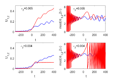
Figure 5: Threshold phenomenon. The upper two panels illustrate double phase-locking in the system for $\epsilon_{2}=0.005$, while in the lower two panels, where $\epsilon_{2}=0.004$, the phase locking with one of the driving components is lost. All other driving parameters in the two cases are the same as in Fig. 4, i.e., $\epsilon_{1}=0.01,\alpha_{1,2}=0.0012,0.0024$.

All remaining dependent variables in the problem, i.e., $V_{1,2}$, $u_{0},u_{11},u_{22},u_{12p},u_{12m},v_{11},v_{22},v_{12p},v_{12m}$, $\Phi_{1,2}$, $\xi$ are related to $U_{1},U_{2}$ (see Eqs. (59-68) in the Appendix). Before proceeding to the analysis of this system, we rewrite Eqs. ((21),(22)) explicitly as differential equations for $\Phi_{1,2}$. We approximate $\omega_{0i}^{2}-\omega_{i}^{2}\approx 2\omega_{0i}(\omega_{0i}-\omega_{i})=2\omega_{0i}(\omega_{di}-\omega_{i}+\alpha_{i}t)=-2\omega_{0i}(\frac{d\Phi_{i}}{dt}-\alpha_{i}t)$, which allows to write these equations as

$$\frac{d\Phi_{1}}{dt} = \alpha_{1}t+\frac{4\sigma(-3\sigma U_{0}^{2}+k_{1}^{2})}{\omega_{01}}U_{1}^{2}+\frac{2k_{1}^{2}\sigma}{\omega_{01}}U_{2}^{2}$$ (23)

$$- \frac{\varepsilon_{1}U_{0}k_{1}^{2}}{2\omega_{01}U_{1}}\cos\Phi_{1},$$

$$\frac{d\Phi_{2}}{dt} = \alpha_{2}t+\frac{4\sigma(-3\sigma U_{0}^{2}+k_{2}^{2})}{\omega_{02}}U_{2}^{2}+\frac{2k_{2}^{2}\sigma}{\omega_{02}}U_{1}^{2}$$ (24)

$$- \frac{\varepsilon_{2}U_{0}k_{2}^{2}}{2\omega_{02}U_{2}}\cos\Phi_{2}.$$

Equations (20),(23), and (24) comprise a complete set of differential equations for studying the dynamics in our problem. By solving this system, and calculating all second-order objects as described above, we obtain a full quasilinear two-phase solution (III,III) of the chirped-driven GP equation. As an illustration, Fig. 5 shows the dynamics of $U_{1,2}$ and $\Phi_{1,2}$ for two cases with the same parameters as in the two lower panels in Fig. 4. The figure illustrates the loss of phase-locking with one of the components of the drive as one passes from $\epsilon_{2}=0.005$ to $0.004$. The upper two panels in Fig. 5 show double phase locking of $\Phi_{1,2}$ at $\pi$ [$mod(2\pi)$] and a continuous autoresonant growth of $U_{1,2}$, while in the lower two panels only $U_{1}$ continues to grow, while $U_{2}$ saturates as $\Phi_{2}$ escapes. Thus, one requires both driving amplitudes to be above some minimal values for a persisting double autoresonance in the system. We discuss this threshold effect in the next section.

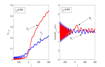
Figure 6: Double phase-locking in the system driven by modulation of the interaction strength. The parameters are the same as in the lower two panels in Fig. 5, but $U_{0}$ in the driving term is replaced by $2\sigma U_{0}^{3}$.

We conclude this section by discussing the case of driving via the modulation of the interaction strength (see the comments at the beginning of Sec. II). It is shown at the end of the Appendix that the reduced system of equations describing two-phase autoresonant formation of space time GP quasicrystals in this case is the same as for the ponderomotive drive (see Eqs. (20),(23),(24)), but $U_{0}$ in the driving terms must be replaced by $2\sigma U_{0}^{3}$. We present an example of such a case in Fig. 6, where the parameters are the same as in the lower two panels in Fig. 5, but the driving is via the interaction strength in the GP equation, as discussed above. One can see two differences between between Fig. 5 and 6. One is that in the case of the interaction strength drive the double phase-locking is restored. This is because effectively the driving amplitude increased by a factor of two, and passed the threshold. The second difference is that the phase mismatches $\Phi_{1,2}$ in Fig. 6 are locked near $0$. The reason is that in this case, there is a new factor of $\sigma$ in the driving perturbation, which for $\sigma=-1$ in this example changes the phase-locking location, as will be discussed in the next Section.

IV Autoresonance conditions and threshold phenomenon

In this section, we discuss conditions for the autoresonant evolution of space-time quasicrystals in BECs. We proceed by defining new (action) variables

$$I_{1,2}=\frac{\omega_{r1,2}U_{1,2}^{2}}{k_{1,2}^{2}}.$$ (25)

Then the system of Eqs. (20,23,24) describing two-phase BECs can be rewritten as

$$\frac{dI_{1}}{dt} = -\eta_{1}\sqrt{I_{1}}\sin\Phi_{1},$$ (26)

$$\frac{dI_{2}}{dt} = -\eta_{2}\sqrt{I_{2}}\sin\Phi_{2},$$ (27)

$$\frac{d\Phi_{1}}{dt} = \sigma(aI_{1}+bI_{2})+\alpha_{1}t-\frac{\eta_{1}}{2\sqrt{I_{1}}}\cos\Phi_{1},$$ (28)

$$\frac{d\Phi_{2}}{dt} = \sigma(bI_{1}+cI_{2})+\alpha_{2}t-\frac{\eta_{2}}{2\sqrt{I_{2}}}\cos\Phi_{2},$$ (29)

where

$$a =\frac{4}{\omega_{r1}^{2}}\left(k_{1}^{2}-3\sigma U_{0}^{2}\right)k_{1}^{2}=\frac{1}{\omega_{r1}^{2}}\left(k_{1}^{4}+3\omega_{r1}^{2}\right),$$

$$b =\frac{2k_{1}^{2}k_{2}^{2}}{\omega_{r1}\omega_{r2}},$$

$$c =\frac{4}{\omega_{r2}^{2}}\left(k_{2}^{2}-3\sigma U_{0}^{2}\right)k_{2}^{2}=\frac{1}{\omega_{r2}^{2}}\left(k_{2}^{4}+3\omega_{r2}^{2}\right),$$

$$\eta_{1,2} =\frac{\varepsilon_{1,2}|k_{1,2}|U_{0}}{\sqrt{\omega_{r1,2}}}.$$

The action-angle Hamiltonian of this system is

$$H(I_{1,2},\Phi_{1,2},t)=\sigma(\frac{a}{2}I_{1}^{2}+bI_{1}I_{2}+\frac{c}{2}I_{2}^{2})$$ (31)

$$+(\alpha_{1}I_{1}+\alpha_{2}I_{2})t-\eta_{1}\sqrt{I_{1}}\cos\Phi_{1}-\eta_{2}\sqrt{I_{2}}\cos\Phi_{2}.$$

Note that as mentioned at the end of Sec. III, in the case of two-phase driving via the modulation of the interaction strength, the system of equations (26)-(29) remains the same, but in the expression for $\eta_{1,2}$, $U_{0}$ must be replaced by $2\sigma U_{0}^{3}$. Finally, a similar system of equations was derived recently in application to Langmuir and ion acoustic waves in plasmas Munirov1 ; Munirov2 .

The autoresonant evolution corresponds to double phase-locking in the system as phase mismatches $\Phi_{1,2}$ remain bounded continuously subject to small initial conditions on $I_{1,2}$ at large negative time $t_{0}$. In the initial stage, the pairs of variables $(I_{1},\Phi_{1})$ and $(I_{2},\Phi_{2})$ decouple and are described by

$$\frac{dI_{i}}{dt}=-\eta_{i}\sqrt{I_{i}}\sin\Phi_{i}$$ (32)

$$\frac{d\Phi_{i}}{dt}=\alpha_{i}t-\frac{\eta_{i}}{2\sqrt{I_{i}}}\cos\Phi_{i}$$ (33)

The phase-locking $\frac{d\Phi_{i}}{dt}\approx 0$ in each of these decoupled systems is guaranteed at large negative times (see Ref. Lazar70 for a detailed analysis) and yields

$$\alpha_{1}t-\frac{\eta_{1}}{2\sqrt{I_{1}}}\cos\Phi_{1}\approx 0,\alpha_{2}t-\frac{\eta_{2}}{2\sqrt{I_{2}}}\cos\Phi_{1}\approx 0$$ (34)

and phase locking at either $\Phi_{1,2}\approx 0$ or $\pi$ if $\alpha_{1,2}$ is negative or positive, respectively, and in both cases $\sqrt{I_{1,2}}\approx-\frac{\eta_{1,2}}{2\left|\alpha_{1,2}\right|t}.$

Next, assuming that the autoresonant phase-locking ($\frac{d\Phi_{i}}{dt}\approx 0$) continues as the system reaches large positive times, in double autoresonance, the actions $I_{1,2}$ are given by the solution of

$$\sigma(aI_{1}+bI_{2})+\alpha_{1}t\approx 0,\sigma(bI_{1}+cI_{2})+\alpha_{2}t\approx 0.$$ (35)

Since coefficients $a,b,c$ are all positive, for having positive solutions for $I_{1,2}$ chirp rates $\alpha_{1,2}$ must have the sign of $-\sigma$, i.e., can be written as $\alpha_{1,2}=-\sigma|\alpha_{1,2}|.$ This yields autoresonant solutions varying linearly in time

$$I_{1}=\frac{c|\alpha_{1}|-b|\alpha_{2}|}{D}t,I_{2}=\frac{a|\alpha_{2}|-b|\alpha_{1}|}{D}t,$$ (36)

where

$$D=ac-b^{2}=\frac{4k_{1}^{2}k_{2}^{2}}{\omega_{r1}^{2}\omega_{r2}^{2}}[4\left(k_{1}^{2}-3\sigma U_{0}^{2}\right)\left(k_{2}^{2}-3\sigma U_{0}^{2}\right)-k_{1}^{2}k_{2}^{2}].$$ (37)

For positivness of both $I_{1,2}$ at large $t$ (large excitations) we must have $c/b>|\alpha_{2}/\alpha_{1}|>b/a$ or

$$\frac{2\omega_{r1}(k_{2}^{2}-3\sigma U_{0}^{2})}{k_{1}^{2}\omega_{r2}}>|\alpha_{2}/\alpha_{1}|>\frac{k_{2}^{2}\omega_{r1}}{2\omega_{r2}(k_{1}^{2}-3\sigma U_{0}^{2})}$$ (38)

Then $D=ac-b^{2}$ must be positive. This is obviously the case for $\sigma=-1$, so we can always find some ratio $|\alpha_{2}/\alpha_{1}|$ in this case for having positive $I_{1,2}$, linearly increasing in time. The case $\sigma=1$ is more complex. Since we still need $D>0$ for having increasing $I_{1,2}$ at large positive times, we must satisfy

$$4\left(k_{1}^{2}-3U_{0}^{2}\right)\left(k_{2}^{2}-3U_{0}^{2}\right)-k_{1}^{2}k_{2}^{2}>0$$ (39)

or

$$\left(1-X\right)\left(1-Y\right)>1/4$$ (40)

where $X=3U_{0}^{2}/k_{2}^{2}$ and $Y=3U_{0}^{2}/k_{1}^{2}$.

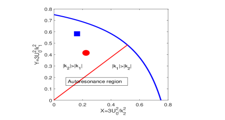
Figure 7: Allowed double phase-locking region for BECs in the case $\sigma=-1$ is below the blue line in the figure. The circle and the square points correspond to parameters $k_{1}=2,k_{2}=-3,U0=0.775$ and $k_{1}=1,k_{2}=-2,U_{0}=0.447$, respectively. The examples of space-time quasicrystals for these two sets of parameters are shown in Fig. 9

The last inequality yields the condition

$$Y<1-\frac{1}{4(1-X)}$$ (41)

The region $S$ in the $(Y,X)$-plane satisfying this inequality (the allowed region) is shown in Fig. 7. Note that in this region $X,Y<3/4$, which guarantees the positivity of $\omega_{r1,2}^{2}$. However, $U_{0}^{2}$ can not be too large to satisfy $X,Y<3/4$ and can be chosen as follows. Let $k_{2}^{2}>$ $k_{1}^{2}$. Then, $X<Y$ and we can choose some value $Y_{0}<3/4$ yielding $U_{0}^{2}=\frac{k_{1}^{2}}{3}Y_{0}$ and $X_{0}=\frac{k_{1}^{2}}{k_{2}^{2}}Y_{0}<\frac{k_{1}^{2}}{k_{2}^{2}}$. This guarantees that the point $(X_{0},Y_{0})$ is inside the allowed region if $Y_{0}<1/2$. However, if $1/2<Y_{0}<3/4$, for having $(X_{0},Y_{0})\in S$ we have a restriction

$$\frac{k_{1}^{2}}{k_{2}^{2}}<\frac{1}{Y_{0}}\left(1-\frac{1}{4(1-Y_{0})}\right).$$ (42)

The inequalities (41) and (42) above are based on the analysis at large positive times and comprise only necesary conditions for synchronized (autoresonant) evolution. We have already discussed the phase-locking at large negative times. However, for synchronized passage through the vicinity of $t=0$, i.e., for having bounded $\Phi_{1,2}$ at all times, in addition to the above, it requires $\eta_{1,2}$ be large enough (for both $\sigma=+1$ and $-1$). In dealing with this issue, we choose some value of‘ $\left|\alpha_{1}\right|$, $\eta_{1}$ and $r=|\alpha_{2}/\alpha_{1}|$ ($r$ must satisfy (38) as described above), which defines $\left|\alpha_{2}\right|$.

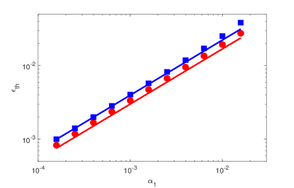
Figure 8: Threshold $\varepsilon_{1th}$ versus $\alpha_{1}$ for autoresonant double phase-locking of BECs in the case $\sigma=-1$ and two sets of parameters, set A: $k_{1}=2,k_{2}=-3,U0=0.775,r=1.08,q=0.7,\mu_{th}=0.403$ (red line) and set B: $k_{1}=1,k_{2}=-2,U_{0}=0.447,r=0.805,q=1.3,\mu_{th}=0.277$ (blue line). The circles and squares show the results of full numerical simulations.

We also fix ratio $q=\eta_{2}/\eta_{1}$, which defines $\eta_{2}$, and we are left with the problem of finding the critical value of $\eta_{1th}$ for autoresonant transition through the vicinity of $t=0$ for this $\left|\alpha_{1}\right|$. Now we return to our original system (26)-(29) and rewrite it as

$$\frac{dJ_{1}}{d\tau} = -\mu\sqrt{J_{1}}\sin\Phi_{1}$$ (43)

$$\frac{dJ_{2}}{d\tau} = -q\mu\sqrt{J_{2}}\sin\Phi_{2}$$ (44)

$$\frac{d\Phi_{1}}{d\tau} = \sigma[(aJ_{1}+bJ_{2})-\tau]-\frac{\mu}{2\sqrt{J_{1}}}\cos\Phi_{1}$$ (45)

$$\frac{d\Phi_{2}}{d\tau} = \sigma[(bJ_{1}+cJ_{2})-r\tau]-\frac{q\mu}{2\sqrt{J_{2}}}\cos\Phi_{2}$$ (46)

where slow time $\tau=\sqrt{\left|\alpha_{1}\right|}t$, $J_{1,2}=I_{1,2}/\sqrt{\left|\alpha_{1}\right|}$ and $\mu=\eta_{1}/\left|\alpha_{1}\right|^{3/4}$.

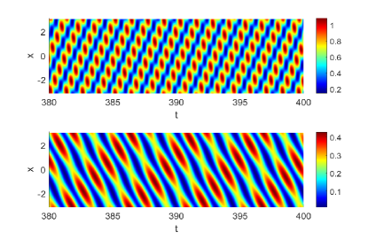
Figure 9: Colormap of space-time BEC quasicrystals for the same two sets of parameters as in Fig. 8, upper panel: set A, lower panel: set B. In both cases $\alpha_{1}=0.001$ and the driving amplitudes are 10% above the threshold.

Therefore, for a given $r$ and $q$, we are left with a single additional parameter $\mu$, and there may exists some minimal value of $\mu_{th}$ in the problem which still guarantees a continuous phase-locking in the system as it passes from large negative times through $t=0$, to large positive times. This value can be found numerically, yielding the minimal (threshold) driving amplitude $\varepsilon_{1th}$ for autoresonance in the system:

$$\varepsilon_{1th}=\mu_{th}\frac{\sqrt{\omega_{r1}}}{\left|k_{1}\right|U_{0}}\left|\alpha_{1}\right|^{3/4}$$ (47)

In the case of driving via modulation strength, the threshold formula remains the same, but $U_{0}$ is replaced by $2U_{0}^{3}$.

We illustrate the characteristic $3/4$ power scaling of $\varepsilon_{1th}$ with $\left|\alpha_{1}\right|$ in Fig. 8, for the parametric driving case, $\sigma=-1$, and two sets of parameters: Set A: $k_{1}=2,k_{2}=-3,U0=0.775,r=1.08,q=0.7$ (red line) and Set B: $k_{1}=1,k_{2}=-2,U_{0}=0.447,r=0.805,q=1.3$ (blue line). The values of $k_{1,2}$ and $U_{0}$ in these two examples correspond to the two points in the allowed autoresonance region in Fig. 7. The circles and squares in Fig. 8 show the results of numerical simulations. Finally, Fig. 10 shows colormaps of $|\varphi|^{2}$ in space-time autoresonant space-time quasicrystals for the same two sets of parameters (the upper and lower panels correspond to sets A and B, respectively). In both cases, $\alpha_{1}=0.001$, and the driving amplitudes are 10% above the thresholds in Fig. 8.

V Conclusions

We have shown that a combination of two independent, small amplitude and chirped frequency parametric-type drivings or modulations of the interaction strength in the GP equation allows controlled nonlinear two-phase excitation of BECs via the process of autoresonance. The amplitude of these excitations grows continuously as the phases of the excited solution follow those of the driving perturbations. The phase-locked excitation process starts from trivial ground state at large negative times and continues as the system passes linear resonances with both driving components at $t=0$ and moves to large positive times. If both driving components are switched off at some large positive time, an ideal, stable space-time quasicrystal is formed, which is periodic in space and aperiodic in time, but preserves long time ordering (see examples of numerical simulations in Figs. 2,4, and 9).

We have developed a weakly nonlinear theory for these two-phase periodic excitations using Whitham’s averaged variational principle, yielding a two degrees of freedom dynamical problem in action-angle variables (see Eqs. (26)-(29)). The analysis of this system at large positive times limits the parameter space for autoresonant excitations (see inequalities (41) and (42). However, these are only necessary conditions for autoresonance in the system. A continuing phase-locking by passage through the linear resonance near $t=0$ requires the driving amplitude to surpass a certain threshold, yielding the sufficient condition for autoresonant excitation. These thresholds scale with the driving frequency chirp rate $\alpha$ as $\sim|\alpha|^{3/4}$ (see Eq.(47)), a relationship corroborated by numerical simulations (see Fig. 8).

Following concepts explored in this study, it seems interesting to investigate autoresonant excitation involving more complex multi-phase quasi-crystalline structures by simultaneously traversing linear resonances with three and more parametric drivings. Furthermore, given that numerous integrable nonlinear PDEs (such as KDV, Sine-Gordon, and more) describing various physical systems allow multiphase solutions, investigating autoresonant formation of space-time quasicrystals in these additional systems through two or more drivings using a similar approach seems interesting. Finally, previous investigations Fajans ; Ido have demonstrated that a sufficiently small dissipation in other applications did not destroy single-phase autoresonant synchronization, but modified the threshold for transition to autoresonance. Investigating the effects of dissipation on autoresonant two-phase BECs is also an important goal for future research.

Appendix: Reduction to two degrees of freedom

We proceed from the Lagrangian density (10) for the ponderomotive drive case

$$L=\frac{1}{2}\left[U_{x}^{2}+U^{2}(V_{x}^{2}+V_{t})\right]-\frac{\sigma}{2}U^{4}-\frac{U^{2}}{2}[\varepsilon_{1}\cos(\theta_{1}-\Phi_{1})-\varepsilon_{2}\cos(\theta_{1}-\Phi_{1})].$$ (48)

The case of driving via the modulation of the interaction strength will be discussed at the end of the Appendix. We average the Lagrangian over $\theta_{1}$ and $\theta_{2}$ between $0$ and $2\pi$ using the weakly nonlinear ansatz (III) and (III). The resulting averaged Lagrangian density $\Lambda$ consists of the following five terms

$$\Lambda_{1} = \left\langle\frac{1}{2}U_{x}^{2}\right\rangle=\frac{1}{4}(k_{1}^{2}U_{1}^{2}+k_{2}^{2}U_{2}^{2})+\frac{1}{4}[2k_{1}k_{2}(u_{12m}^{2}-u_{12p}^{2})$$

$$+k_{1}^{2}(4u_{11}^{2}+u_{12m}^{2}+u_{12p}^{2})+k_{2}^{2}(u_{12m}^{2}+u_{12p}^{2}+4u_{22}^{2})],$$

$$\Lambda_{2} = \left\langle\frac{1}{2}U_{x}^{2}\right\rangle=\frac{U_{0}^{2}}{4}(k_{1}^{2}V_{1}^{2}+k_{2}^{2}V_{2}^{2})+\frac{1}{16}[k_{1}^{2}(8u_{0}U_{0}V_{1}^{2}+3U_{1}^{2}V_{1}^{2}$$

$$+4U_{0}u_{11}V_{1}^{2}+2U_{2}^{2}V_{1}^{2}+16U_{0}U_{1}V_{1}v_{11}+16U_{0}^{2}v_{11}^{2}-$$

$$8U_{0}(U_{2}V_{1}(v_{12m}-v_{12p})+(u_{12m}V_{1}+u_{12p}V_{1}+U_{1}(v_{12m}+v_{12p}))V_{2}))$$

$$+k_{2}^{2}((2U_{1}^{2}+3U_{2}^{2})V_{2}^{2}+4U_{0}V_{2}(-2U_{1}v_{12m}+2U_{1}v_{12p}+2u_{0}V_{2}+u_{22}V_{2})$$

$$+4U_{0}^{2}(v_{12m}^{2}+v_{12p}^{2}+4v_{22}^{2}))],$$

$$\Lambda_{3} = \left\langle\frac{1}{2}U^{2}V_{t}\right\rangle=\sigma U_{0}^{4}+\frac{1}{4}(2\gamma U_{0}^{2}+2U_{0}(\sigma U_{0}(4u_{0}U_{0}+U_{1}^{2}+U_{2}^{2})-\omega_{1}U_{1}V_{1}-\omega_{2}U_{2}V_{2}))+$$

$$\frac{1}{4}[\gamma(4u_{0}U_{0}+U_{1}^{2}+U_{2}^{2})+2\sigma U_{0}^{2}(2u_{0}^{2}+u_{11}^{2}+u_{12m}^{2}+u_{12p}^{2}+u_{22}^{2})-\omega_{1}(2u_{0}+u_{11})U_{1}V_{1}+$$

$$(u_{12m}+u_{12p})U_{2}V_{1}-U_{1}^{2}v_{11}-4U_{0}u_{11}v_{11}-2U_{0}u_{12m}v_{12m}-2U_{0}u_{12p}v_{12p}+U_{1}U_{2}(v_{12m}+v_{12p}))+$$

$$\omega_{2}(U_{1}U_{2}(v_{12m}-v_{12p})+(u_{12m}+u_{12p})U_{1}V_{2}-(2u_{0}+u_{22})U_{2}V_{2}+U_{2}v_{22})+$$

$$U_{0}(-2u_{12m}v_{12m}+2u_{12p}v_{12p}+4u_{22}v_{22}))],$$

$$\Lambda_{4} = \left\langle-\frac{\sigma}{2}U^{4}\right\rangle=\frac{\sigma}{2}U_{0}^{4}-\frac{\sigma}{2}U_{0}^{2}(4u_{0}U_{0}+3(U_{1}^{2}+U_{2}^{2}))-$$

$$\frac{3\sigma}{16}[16u_{0}^{2}U_{0}^{2}+U_{1}^{4}-16U_{0}U_{1}(u_{12m}+u_{12p})U_{2}+U_{2}^{4}+16u_{0}U_{0}(U_{1}^{2}+U_{2}^{2})+$$

$$4U_{1}^{2}(2U_{0}u_{11}+U_{2}^{2})+8U_{0}(U_{2}^{2}u22+U_{0}(u_{11}^{2}+u_{12m}^{2}+u_{12p}^{2}+u_{22}^{2}))],$$

$$\Lambda_{5}=\left\langle-\frac{U^{2}}{2}[\varepsilon_{1}\cos(\theta_{1}-\Phi_{1})-\varepsilon_{2}\cos(\theta_{1}-\Phi_{1})]\right\rangle=-\frac{U_{0}}{2}(\varepsilon_{1}U_{1}\cos\Phi_{1}+\varepsilon_{2}U_{2}\cos\Phi_{2}),$$ (53)

where we have expanded to 4-th order in amplitudes in Eqs. (Appendix: Reduction to two degrees of freedom)-(Appendix: Reduction to two degrees of freedom) and to first-order in Eq. (53), assuming $\varepsilon_{1,2}$ are sufficiently small. Note that except in $\Lambda_{5}$, the averaged Lagrangian density $\Lambda$ includes only second and fourth-order terms in the square brackets. Also note that $\Lambda$ does not include the time derivatives with respect to the amplitudes, and therefore, the variations with respect to each of these $13$ amplitudes are simply $\partial\Lambda/\partial A_{i}=0$, where $A_{i}$ is the set of these amplitudes.

As the next step, we consider the linearized problem, i.e., neglect all fourth-order terms in $\Lambda$. Then the variations with respect to $U_{1,2}$ and $V_{1,2}$ yield

$$(k_{i}^{2}-4\sigma U_{0}^{2})U_{i}-\omega_{i}U_{0}V_{i}-\varepsilon_{i}U_{0}\cos\Phi_{i} = 0$$ (54)

$$k_{i}^{2}U_{0}V_{i}-\omega_{i}U_{i} = 0$$ (55)

with solutions

$$V_{i}=\frac{\varepsilon\omega_{i}}{(\omega_{0i}^{2}-\omega_{i}^{2})}\cos\Phi_{i},U_{i}=\frac{k_{i}^{2}U_{0}}{\omega_{i}}V_{i}$$ (56)

which is a generalization of Eqs. (15) and (16) for the case of ideal phase locking, ($\omega_{i}=\omega_{di}$ and $\Phi_{i}=0$).

The next step is the inclusion of nonlinearities and taking variations of the full averaged Lagrangian density $\Lambda$ with respect to $u_{0}$ and $\xi$ yielding

$$\frac{\partial\Lambda}{\partial u_{0}}=\gamma U_{0}-\sigma(4u_{0}U_{0}^{2}+3U_{0}(U_{1}^{2}+U_{2}^{2}))-\frac{1}{2}(\omega_{1}U_{1}V_{1}-k_{1}^{2}U_{0}V_{1}^{2}+\omega_{2}U_{2}V_{2}-k_{2}^{2}U_{0}V_{2}^{2})=0,$$ (57)

$$\frac{d}{dt}\left(\frac{\partial\Lambda}{\partial\gamma}\right)=\frac{d}{dt}(4u_{0}U_{0}+U_{1}^{2}+U_{2}^{2})=0.$$ (58)

Then

$$u_{0} = -\frac{(U_{1}^{2}+U_{2}^{2})}{4U_{0}},$$ (59)

$$\gamma = 2\sigma(U_{1}^{2}+U_{2}^{2})+\frac{1}{2}(\omega_{1}\frac{U_{1}V_{1}}{U_{0}}-k_{1}^{2}V_{1}^{2}+\omega_{2}\frac{U_{2}V_{2}}{U_{0}}-k_{2}^{2}V_{2}^{2}).$$ (60)

In these second order results, assuming proximity to the linear resonances, we replace $\omega_{1,2}$ with the linear resonance frequencies $\omega_{01,02}$ (see Eq. (17)) and $V_{i}$ with its linear relation $V_{0i}=\frac{\omega_{i}}{k_{i}^{2}U_{0}}U_{i}$. Then, the term in the brackets in the last equation vanishes and one gets:

$$\gamma=2\sigma(U_{1}^{2}+U_{2}^{2}).$$ (61)

Next, we take variations with respect to the remaining second-order amplitudes, make the same replacements for $\omega_{1,2}$ and $V_{i}$ as above and obtain

$$u_{ii}=-\frac{k_{i}^{2}+8\sigma U_{0}^{2}}{4U_{0}k_{i}^{2}}U_{i}^{2},$$ (62)

$$v_{ii}=-\frac{\sqrt{k_{i}^{2}-4\sigma U_{0}^{2}}(k_{i}^{2}-2\sigma U_{0}^{2})}{2k_{i}^{3}U_{0}^{2}}U_{i}^{2},$$ (63)

$$u_{12p}=\frac{(4\sigma U_{0}^{2}+\sqrt{k_{1}^{2}-4\sigma U_{0}^{2}})\sqrt{k_{1}^{2}-4\sigma U_{0}^{2}}U_{1}U_{2}}{2k_{1}k_{2}U_{0}},u_{12m}=-u_{12p},$$ (64)

$$v_{1p}=\frac{k_{1}^{2}\sqrt{k_{2}^{2}-4\sigma U_{0}^{2}}-k_{2}^{2}\sqrt{k_{1}^{2}-4\sigma U_{0}^{2}}+(k_{1}k_{2}+4\sigma U_{0}^{2})(\sqrt{k_{1}^{2}-4\sigma U_{0}^{2}}-\sqrt{k_{2}^{2}-4\sigma U_{0}^{2}})}{2k_{1}k_{2}(k_{1}-k_{2})U_{0}^{2}}U_{1}U_{2},$$ (65)

$$v_{1m}=\frac{-k_{1}^{2}\sqrt{k_{2}^{2}-4\sigma U_{0}^{2}}+k_{2}^{2}\sqrt{k_{1}^{2}-4\sigma U_{0}^{2}}+(k_{1}k_{2}-4\sigma U_{0}^{2})(\sqrt{k_{1}^{2}-4\sigma U_{0}^{2}}-\sqrt{k_{2}^{2}-4\sigma U_{0}^{2}})}{2k_{1}k_{2}(k_{1}-k_{2})U_{0}^{2}}U_{1}U_{2}.$$ (66)

At this stage, we take variations with respect to $V_{i}$, solve the resulting algebraic equation for $V_{i}$, and replace again $\omega_{1,2}$ and $V_{i}$ in the nonlinear part of the solution by $\omega_{01,02}$ and $V_{0i}=\frac{\omega_{i}}{k_{i}^{2}U_{0}}U_{i}$. This results in:

$$V_{1}=\frac{k_{1}\omega_{1}U_{0}^{2}U_{1}-(3\sigma U_{0}^{2}U_{1}^{3}-k_{1}^{2}U_{1}(\frac{5}{8}U_{1}^{2}+\frac{3}{4}U_{2}^{2}))\sqrt{k_{1}^{2}-4\sigma U_{0}^{2}}}{k_{1}^{3}U_{0}^{3}},$$ (67)

$$V_{2}=\frac{k_{2}\omega_{2}U_{0}^{2}U_{2}+(3\sigma U_{0}^{2}U_{2}^{3}-k_{2}^{2}U_{2}(\frac{3}{4}U_{1}^{2}+\frac{5}{8}U_{2}^{2}))\sqrt{k_{2}^{2}-4\sigma U_{0}^{2}}}{k_{2}^{3}U_{0}^{3}}.$$ (68)

Note that these solutions involve first-order linear parts and third-order nonlinear corrections.

Finally, we take variation with respect to $U_{i}$ to get

$$(k_{1}^{2}-8\sigma U_{0}^{2})U_{1}-\omega_{1}U_{0}V_{1}+Q_{1}-\varepsilon_{1}U_{0}\cos\Phi_{1} = 0,$$ (69)

$$(k_{2}^{2}-8\sigma U_{0}^{2})U_{2}-\omega_{2}U_{0}V_{2}+Q_{2}-\varepsilon_{2}U_{0}\cos\Phi_{2} = 0,$$ (70)

where $Q_{i}$ are third-order nonlinear corrections (similar to those in Eqs. (67),(68)). The last two equations can be simplified as follows: In the nonlinear part of these equations, we again replace $\omega_{1,2}$ and $V_{i}$ by $\omega_{01,2}$ and $V_{0i}=\frac{\omega_{i}}{k_{i}^{2}U_{0}}U_{i}$. Additionally, we replace $V_{i}$ in the linear parts of (69) and (70) by the expressions in (67),(68). The algebra involved in these manipulations is done via Mathematica package yielding two equations:

$$(\omega_{01}^{2}-\omega_{1}^{2})U_{1}-24U_{0}^{2}U_{1}^{3}+4k_{1}^{2}\sigma U_{1}(2U_{1}^{2}+U_{2}^{2})-\varepsilon_{1}U_{0}k_{1}^{2}\cos\Phi_{1} = 0.$$ (71)

$$(\omega_{02}^{2}-\omega_{2}^{2})U_{2}-24U_{0}^{2}U_{2}^{3}+4k_{2}^{2}\sigma U_{2}(2U_{2}^{2}+U_{1}^{2})-\varepsilon_{2}U_{0}k_{2}^{2}\cos\Phi_{2} = 0.$$ (72)

Finally, we need additional two equations for our reduced system describing $U_{i}$ and $\Phi_{i}$. These equations are obtained by variation with respect to $\theta_{i}$. Since $\Phi_{i}(t)=\theta_{i}-\theta_{di}$, and $d\theta_{i}/dt=\omega_{i}$, we get

$$\frac{d}{dt}\frac{\partial\Lambda}{\partial\omega_{i}}=\frac{\partial\Lambda}{\partial\Phi_{i}},$$ (73)

which to lowest significant order yields

$$\frac{dU_{i}}{dt}=-\frac{\varepsilon_{i}U_{0}k_{i}^{2}}{2\omega_{0i}}\sin\Phi_{i}.$$ (74)

We conclude this Appendix by discussing the case of driving via the interaction strength in the GP equation. In this case, the driving term in the Laplacian (48) changes (see the discussion at the beginning of Sec. II) and the Laplacian becomes

$$L=\frac{1}{2}\left[U_{x}^{2}+U^{2}(V_{x}^{2}+V_{t})\right]-\frac{\sigma}{2}U^{4}-\frac{\sigma U^{4}}{2}[\varepsilon_{1}\cos(\theta_{1}-\Phi_{1})-\varepsilon_{2}\cos(\theta_{1}-\Phi_{1})].$$ (75)

This change affects only the driving term $\Lambda_{5}$ (see Eq. (53) in the averaged Laplacian, transforming it to

$$\Lambda_{5}=-\sigma U_{0}^{3}(\varepsilon_{1}U_{1}\cos\Phi_{1}+\varepsilon_{2}U_{2}\cos\Phi_{2}).$$ (76)

Formally, this is a replacement of $U_{0}$ in the coefficient from the ponderomotive drive case by $2\sigma U_{0}^{3}$. The same replacement should be done in the case of driving via interaction strength in all driving terms in the reduced system of equations (71),(72),(74).

References

(1) D. Shechtman, I. Blech, D. Gratias, and J. W. Cahn, Phys. Rev. Lett. 53, 1951 (1984).
(2) D. Levine, P. J. Steinhardt, Phys. Rev. Lett.
53, 2477 (1984).
(3) M. Senechal, Quasicrystals and Geometry (Cambridge University Press, Cambridge, England, 1995).
(4) S. Autti, V. B. Eltsov and G. E. Volovik, Phys. Rev. Lett.120,
215301 (2018).
(5) A. J. E. Kreil, H. Yu. Musiienko-Shmarova, S. Eggert, A. A. Serga, B. Hillebrands, D. A. Bozhko, A. Pomyalov, and V. S. L’vov, Phys. Rev. B 100, 020406(R) (2019).
(6) K. Giergiel, A. Kuros, and K. Sacha, Phys. Rev. B 99, 220303(R) (2019).
(7) J. G. Cosme, J. Skulte and L. Mathey, Phys Rev A 100, 053615 (2019).
(8) A. Scott, Nonlinear Science: Emergence and Dynamics of Coherent Structures (Oxford University Press, New York,1999).
(9) S. Novikov, S.V. Manakov, L. P. Pitaevskii, and V.E. Zacharov, Theory of Solitons (Consultants Bureau, New York,1984).
(10) L. Friedland, Scholarpedia 4(1), 5473 (2009).
(11) L. Friedland, A.G. Shagalov, Phys. Rev. Lett. 90, 074101 (2003).
(12) L. Friedland, A. G. Shagalov, Phys. Rev. E 71, 036206 (2005).
(13) A. G. Shagalov, L. Friedland, Physica D 238, 1561 (2009).
(14) V. R. Munirov, L. Friedland, and J.S. Wurtele, Phys. Rev. E 106, 055201 (2022).
(15) V. R. Munirov, L. Friedland, and J.S. Wurtele, Phys. Rev. Research 4, 023150 (2022).
(16) G. B. Whitham, Linear and Nonlinear Waves (John Wiley, NewYork, 1973).
(17) F. Dalfovo, S. Giorgini, L.P. Pitaevskii, S. Stringari, Rev. Mod. Phys., 71, 463 (1999).
(18) R. Yamazaki, S. Taie, S. Sugawa, Y. Takahashi, Phys. Rev. Lett. 105, 050405 (2010).
(19) J. Schloss, P. Barnett, R. Sachdeva, T. Busch, Phys. Rev A 102, 043325 (2020).
(20) C-X. Zhu, W. Yi, G-C. Guo, Z-W. Zhou, Phys. Rev A 99, 023619 (2019).
(21) A. G. Shagalov and L. Friedland, Phys. Rev. E 109, 014201 (2024).
(22) A. J. Leggett, Rev. Mod. Phys., 73, 301 (2001).
(23) V. Zakharov, L. Ostrovsky, Physica D: Nonlinear Phenomena 238, 540 (2009).
(24) G. P. Agrawal, Nonlinear Fiber Optics (4th ed.) (Academic Press, San Diego, 2007) p. 121.
(25) A.G. Shagalov and L. Friedland, Phys. Rev. E, 106,024211(2022).
(26) L. Friedland, Phys. Fluids B4, 3199 (1992).
(27) J. Fajans, E. Gilson, and L. Friedland, Phys. Plasmas 8, 423 (2001).
(28) I. Barth, L. Friedland, E. Sarid, and A.G. Shagalov, Phys. Rev. Lett. 103, 155001 (2009).