SyncTweedies: A General Generative Framework Based on Synchronized Diffusions

Abstract

We introduce a general framework for generating diverse visual content, including ambiguous images, panorama images, mesh textures, and Gaussian splat textures, by synchronizing multiple diffusion processes. We present exhaustive investigation into all possible scenarios for synchronizing multiple diffusion processes through a canonical space and analyze their characteristics across applications. In doing so, we reveal a previously unexplored case: averaging the outputs of Tweedie’s formula while conducting denoising in multiple instance spaces. This case also provides the best quality with the widest applicability to downstream tasks. We name this case SyncTweedies. In our experiments generating visual content aforementioned, we demonstrate the superior quality of generation by SyncTweedies compared to other synchronization methods, optimization-based and iterative-update-based methods.

Figure 1: Diverse visual content generated by SyncTweedies: A training-free, synchronized diffusion process with broad applicability.

1 Introduction

Image diffusion models [40, 31] have shown unprecedented ability to generate plausible images that are indistinguishable from real ones. The generative power of these models stems not only from their capacity to memorize a vast diversity of potential data but also from being trained on Internet-scale image datasets.

Our goal is to expand the capabilities of pretrained image diffusion models to produce a wide range of 2D and 3D visual content, including panoramic images and textures for 3D objects, without the need to train diffusion models from scratch for each specific visual content. Despite the existence of general image datasets on the scale of billions [41], collecting other forms of visual data at this scale is not feasible. Nonetheless, most visual content can be converted into a regular image of a specific size through certain mappings, such as cropping for panoramic images and rendering for textures of 3D objects. Thus, we employ such a bridging function between each type of visual content and images, along with standard image diffusion models like StableDiffusion [40] and Midjourney [31], to generate a diverse range of visual content.

We introduce a general generative framework that generates data points in the desired visual content space—referred to as canonical space—by combining the denoising process of diffusion models in the conventional image space—referred to as instance spaces. Given the bridging functions connecting the canonical space and instance spaces, we first explore performing individual denoising processes in each instance space while synchronizing them in the canonical space via the mapping. Another approach is to denoise directly in the canonical space, although it is not immediately feasible due to the absence of diffusion models trained on the canonical space. We investigate redirecting the noise prediction to the instance spaces but aggregating the outputs later in the canonical space.

Depending on the timing of aggregating the outputs of computation in the instance spaces, we observe five main possible options for the joint denoising processes—many other options are also feasible but show inferior performance, as discussed in the supplementary material. Previous works [4, 11, 29] have investigated each of the possible cases only for specific applications, but none of them has attempted to analyze and compare them across a range of applications. For the first time, we analyze all the possible options of joint denoising processes in multiple applications, including ambiguous image generation, panorama generation, mesh texturing, and Gaussian splatting texturing, and compare their performance. To this end, we demonstrate that the approach, which has not been attempted in any previous work, of conducting denoising processes in instance spaces (not the canonical space) and synchronizing the outputs of Tweedie’s formula [39] in the canonical space, provides the broadest applicability across a range of applications and the best performance. We name this approach SyncTweedies and showcase its state-of-the-art performance in multiple visual content creation tasks compared with previous methods.

When it comes to generating visual content that can be parameterized into an image, a notable approach not utilizing joint diffusion is Score Distillation Sampling (SDS) [35], which has shown particular effectiveness in 3D generation and texturing. However, this alternative application of diffusion models has been observed to produce suboptimal results and also requires a high CFG [17] weight for convergence, leading to over-saturation. For 3D texture generation, specifically, an approach that iteratively updates each view image has also been explored in multiple previous works [8, 38]. However, the accumulation of errors over iterations has been identified as a challenge. We demonstrate that our diffusion synchronization-based approach outperforms these methods in terms of generation quality across various applications while also achieving faster runtime.

2 Problem Definition

We consider a generative process that samples data within a space we term the canonical space $\mathcal{Z}$, where a pretrained diffusion model is not provided. Instead, we leverage diffusion models trained in other spaces called the instance spaces $\{\mathcal{W}_{i}\}_{i=1:N}$, where a subset of the canonical space can be instantiated into each of them via a mapping: $f_{i}:\mathcal{Z}\rightarrow\mathcal{W}_{i}$; we refer to this mapping as the projection. Let $g_{i}$ denote the unprojection, which is the inverse of $f_{i}$, mapping the instance space to a subset of the canonical space. We assume that the entire canonical space $\mathcal{Z}$ can be expressed as a composition of multiple instance spaces ${\mathcal{W}_{i}}$, meaning that for any data point $\mathbf{z}\in\mathcal{Z}$, there exist $\{\mathbf{w}_{i}\,|\,\mathbf{w}_{i}\in\mathcal{W}_{i}\}_{i=1:N}$ such that

$$\mathbf{z}=\mathcal{A}\left(\{g_{i}(\mathbf{w}_{i})\}_{i=1:N}\right),$$ (1)

where $\mathcal{A}$ is an aggregation function that averages the data points from the multiple instance spaces in the canonical space. Our objective is to introduce a general framework for the generative process in the canonical space by integrating multiple denoising processes from different instance spaces through synchronization.

3 Joint Diffusion Synchronization

We outline the denoising procedures of representative diffusion models, DDIM [42] and DDPM [16], and present possible options for joint diffusion processes.

3.1 Denoising Process of DDIM [42] and DDPM [16]

Song et al.  [42] have proposed DDIM, a generalized denoising process that controls the level of randomness during denoising. DDIM [42] is based on non-Markovian forward processes as follows:

$$q_{\sigma_{t}}\left(\mathbf{x}^{(t)}|\mathbf{x}^{(t-1)},\mathbf{x}^{(0)}\right)=\frac{q_{\sigma_{t}}\left(\mathbf{x}^{(t-1)}|\mathbf{x}^{(t)},\mathbf{x}^{(0)}\right)q\left(\mathbf{x}^{(t)}|\mathbf{x}^{(0)}\right)}{q\left(\mathbf{x}^{(t-1)}|\mathbf{x}^{(0)}\right)},$$ (2)

where $\sigma_{t}$ is a hyperparamter determining the level of randomness, $\mathbf{x}^{(0)}$ is a clean data point, and $\mathbf{x}^{(t)}$ is its noise-perturbed data at timestep $t$. Here, sampling $\mathbf{x}^{(t)}$ from $\mathbf{x}^{(t-1)}$ takes into account both the current noisy data point $\mathbf{x}^{(t-1)}$ and the original data point $\mathbf{x}^{(0)}$. In Equation 2, to satisfy $q\left(\mathbf{x}^{(t)}|\mathbf{x}^{(0)}\right)=\mathcal{N}\left(\sqrt{\alpha_{t}}\mathbf{x}^{(0)},(1-\alpha_{t})\mathbf{I}\right)$, following DDPM [16], the posterior of the forward process $q_{\sigma_{t}}\left(\mathbf{x}^{(t-1)}|\mathbf{x}^{(t)},\mathbf{x}^{(0)}\right)$ is chosen as follows:

$$q_{\sigma_{t}}\left(\mathbf{x}^{(t-1)}|\mathbf{x}^{(t)},\mathbf{x}^{(0)}\right)=\mathcal{N}\left(\psi^{(t)}_{\sigma_{t}}(\mathbf{x}^{(t)},\mathbf{x}^{(0)}),\sigma_{t}^{2}\mathbf{I}\right),$$ (3)

where $\psi_{\sigma_{t}}^{(t)}(\mathbf{x}^{(t)},\mathbf{x}^{(0)})=\sqrt{\alpha_{t-1}}\mathbf{x}^{(0)}+\sqrt{\frac{1-\alpha_{t-1}-\sigma_{t}^{2}}{1-\alpha_{t}}}\cdot(\mathbf{x}^{(t)}-\sqrt{\alpha_{t}}\mathbf{x}^{(0)}$).

When $\sigma_{t}=0$ for all $t$, the denoising process becomes deterministic. Also, note that the denoising process of DDPM [16] is a special case of DDIM [42] when $\sigma_{t}=\sqrt{(1-\alpha_{t-1})(1-\alpha_{t})(1-\alpha_{t}/\alpha_{t-1}})$.

While $\mathbf{x}^{(t-1)}$ can be sampled from the given $\mathbf{x}^{(t)}$ and $\mathbf{x}^{(0)}$ based on Equation 3, the original clean data point $\mathbf{x}^{(0)}$ is unknown. Thus, it is approximated using a noise prediction neural network, denoted as $\boldsymbol{\epsilon}_{\theta}$. Given the noisy data point $\mathbf{x}^{(t)}$, we compute a one-step denoised estimate of $\mathbf{x}^{(0)}$ using Tweedie’s formula [39]:

$$\mathbf{x}^{(0)}\simeq\phi^{(t)}(\mathbf{x}^{(t)},\boldsymbol{\epsilon}_{\theta}(\mathbf{x}^{(t)})) =\frac{\mathbf{x}^{(t)}-\sqrt{1-\alpha_{t}}\boldsymbol{\epsilon}_{\theta}(\mathbf{x}^{(t)})}{\sqrt{\alpha_{t}}}.$$ (4)

For simplicity, the time input and condition term in $\boldsymbol{\epsilon}_{\theta}$ are omitted. In short, each denoising step of DDIM [42] is expressed as follows:

$$\mathbf{x}^{(t-1)}=\psi^{(t)}_{\sigma_{t}}(\mathbf{x}^{(t)},\phi^{(t)}(\mathbf{x}^{(t)},\boldsymbol{\epsilon}_{\theta}(\mathbf{x}^{(t)})))+\sigma_{t}\boldsymbol{\epsilon},\quad\text{where}\,\,\boldsymbol{\epsilon}\sim\mathcal{N}(\mathbf{0},\mathbf{I}).\vspace{-0.5\baselineskip}$$ (5)

3.2 Synchronized Joint Denoising Processes

We now explore various scenarios of sampling $\mathbf{z}\in\mathcal{Z}$ by leveraging the composition of multiple denoising processes in the instance spaces $\{\mathcal{W}_{i}\}_{i=1:N}$. Consider the denoising step of the diffusion model at each time step $t$ in each instance space $\mathcal{W}_{i}$:

$$\mathbf{w}_{i}^{(t-1)}=\psi^{(t)}_{\sigma_{t}}(\mathbf{w}_{i}^{(t)},\phi^{(t)}(\mathbf{w}_{i}^{(t)},\boldsymbol{\epsilon}_{\theta}(\mathbf{w}_{i}^{(t)})))+\sigma_{t}\boldsymbol{\epsilon}.$$ (6)

A naïve approach to generate data in the canonical space through the denoising process in instance spaces would be to perform the process independently in each instance space and then aggregate the generated output in the canonical space at the end using the averaging function $\mathcal{A}$. However, this approach results in poor outcomes that lack consistency across outputs in different instance spaces. Hence, we propose to synchronize the denoising processes at each time step $t$ through the unprojection operation from each instance space to the canonical space $g_{i}$ and the aggregation operation $\mathcal{A}$, after which the results will be back-projected via the projection operation $f_{i}$ to each instance space again.

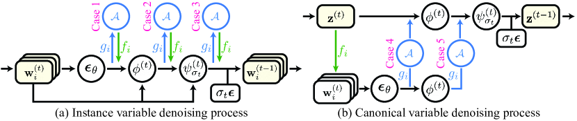
Figure 2: Diagrams of joint diffusion processes. The left diagram depicts a joint diffusion process that denoises instance variables $\{\mathbf{w}_{i}\}$ while the right diagram illustrates a diffusion process that directly denoises a canonical variable $\mathbf{z}$.

Note that, as described in Equation 5, the estimated mean $\psi^{(t)}_{\sigma_{t}}(\cdot,\cdot)$ of the posterior distribution involves multiple layers of computations: noise prediction $\boldsymbol{\epsilon}_{\theta}(\cdot)$, Tweedie’s formula [39] $\phi^{(t)}(\cdot,\cdot)$ approximating the final output $x^{(0)}$ each time step, and the final linear combination $\psi^{(t)}_{\sigma_{t}}(\cdot,\cdot)$. Synchronization through the sequence of unprojection $g_{i}$, aggregation in the canonical space $\mathcal{A}$, and projection $f_{i}$ can thus be performed after each layer of these computations, resulting in the following three cases:

1. : $\mathbf{w}_{i}^{(t-1)}=\psi^{(t)}_{\sigma_{t}}(\mathbf{w}_{i}^{(t)},\phi^{(t)}(\mathbf{w}_{i}^{(t)},{\color[rgb]{0.19921875,0.5703125,0.15625}f_{i}}({\color[rgb]{0,0.5,1}\mathcal{A}}(\{{\color[rgb]{0,0.5,1}g_{j}}({\color[rgb]{1,0,0.5}\boldsymbol{\epsilon}_{\theta}}(\mathbf{w}_{j}^{(t)}))\}_{j=1}^{N}))))+\sigma_{t}\boldsymbol{\epsilon}$

2. : $\mathbf{w}_{i}^{(t-1)}=\psi^{(t)}_{\sigma_{t}}(\mathbf{w}_{i}^{(t)},{\color[rgb]{0.19921875,0.5703125,0.15625}f_{i}}({\color[rgb]{0,0.5,1}\mathcal{A}}(\{{\color[rgb]{0,0.5,1}g_{j}}({\color[rgb]{1,0,0.5}\phi^{(t)}}(\mathbf{w}_{j}^{(t)},\boldsymbol{\epsilon}_{\theta}(\mathbf{w}_{j}^{(t)})))\}_{j=1}^{N}))+\sigma_{t}\boldsymbol{\epsilon}$

3. : $\mathbf{w}_{i}^{(t-1)}={\color[rgb]{0.19921875,0.5703125,0.15625}f_{i}}({\color[rgb]{0,0.5,1}\mathcal{A}}(\{{\color[rgb]{0,0.5,1}g_{j}}({\color[rgb]{1,0,0.5}\psi^{(t)}_{\sigma_{t}}}(\mathbf{w}_{j}^{(t)},\phi^{(t)}(\mathbf{w}_{j}^{(t)},\boldsymbol{\epsilon}_{\theta}(\mathbf{w}_{j}^{(t)}))))\}_{j=1}^{N}))+\sigma_{t}\boldsymbol{\epsilon}$.

In each case, we highlight the computation layer to be synchronized in red. The final outputs $\mathbf{w}_{i}^{(0)}$ are also synchronized at the end through the canonical space.

Another notable approach is to conduct the denoising process directly on the canonical space:

$$\mathbf{z}^{(t-1)}=\psi^{(t)}_{\sigma_{t}}(\mathbf{z}^{(t)},\phi^{(t)}(\mathbf{z}^{(t)},\boldsymbol{\epsilon}_{\theta}(\mathbf{z}^{(t)}))))+\sigma_{t}\boldsymbol{\epsilon},$$ (7)

although it is not directly feasible because the noise prediction network in the canonical space $\boldsymbol{\epsilon}_{\theta}(\mathbf{z}^{(t)})$ is not trained. Nevertheless, it can be achieved by redirecting the noise prediction to the instance spaces as follows:

1. project the intermediate noisy data point $\mathbf{z}^{(t)}$ from the canonical space to each instance space, resulting in $f_{i}(\mathbf{z}^{(t)})$,

2. apply a subsequence of the operations: $\boldsymbol{\epsilon}_{\theta}$, $\phi^{(t)}$, and $\psi^{(t)}_{\sigma_{t}}$,

3. unproject the outputs back to the canonical space via $g_{i}$ and then average them using the aggregation function $\mathcal{A}$, and

4. perform the remaining operations in the canonical space.

Such an approach of performing the denoising process in the canonical space leads to the following two additional cases depending on the subsequence of operations at step (b):

1. : $\mathbf{z}^{(t-1)}=\psi^{(t)}_{\sigma_{t}}(\mathbf{z}^{(t)},\phi^{(t)}(\mathbf{z}^{(t)},{\color[rgb]{0,0.5,1}\mathcal{A}}(\{{\color[rgb]{0,0.5,1}g_{i}}({\color[rgb]{1,0,0.5}\boldsymbol{\epsilon}_{\theta}}({\color[rgb]{0.19921875,0.5703125,0.15625}f_{i}}(\mathbf{z}^{(t)})))\}_{i=1}^{N}))))+\sigma_{t}\boldsymbol{\epsilon}$

2. : $\mathbf{z}^{(t-1)}=\psi^{(t)}_{\sigma_{t}}(\mathbf{z}^{(t)},{\color[rgb]{0,0.5,1}\mathcal{A}}(\{{\color[rgb]{0,0.5,1}g_{i}}({\color[rgb]{1,0,0.5}\phi^{(t)}}({\color[rgb]{0.19921875,0.5703125,0.15625}f_{i}}(\mathbf{z}^{(t)}),\boldsymbol{\epsilon}_{\theta}({\color[rgb]{0.19921875,0.5703125,0.15625}f_{i}}(\mathbf{z}^{(t)}))))\}_{i=1}^{N}))+\sigma_{t}\boldsymbol{\epsilon}$.

Note the analogy between Case 1 and Case 4, and Case 2 and Case 5 in terms of the information averaged in the canonical space with the aggregation operator $\mathcal{A}$: either the outputs of $\boldsymbol{\epsilon}_{\theta}(\cdot)$ or $\phi^{(t)}(\cdot,\cdot)$. The following is also a viable option:

$$\mathbf{z}^{(t-1)}={\color[rgb]{0,0.5,1}\mathcal{A}}(\{{\color[rgb]{0,0.5,1}g_{i}}({\color[rgb]{1,0,0.5}\psi^{(t)}_{\sigma_{t}}}({\color[rgb]{0.19921875,0.5703125,0.15625}f_{i}}(\mathbf{z}^{(t)}),\phi^{(t)}({\color[rgb]{0.19921875,0.5703125,0.15625}f_{i}}(\mathbf{z}^{(t)}),\boldsymbol{\epsilon}_{\theta}({\color[rgb]{0.19921875,0.5703125,0.15625}f_{i}}(\mathbf{z}^{(t)})))))\}_{i=1}^{N})+\sigma_{t}\boldsymbol{\epsilon}.$$ (8)

but in turn, it is identical to Case 3 except for the initial step particularly when $\sigma_{t}=0$ for all $t$. The difference between the formulations of the two cases lies in whether the projection $f_{i}$ is conducted at the end of each denoising step or at the beginning, resulting in only a distinction in initialization, whether initializing $\{\mathbf{w}_{i}^{(T)}\}_{i=1:N}$ or $\mathbf{z}^{(T)}$. We discuss this as Case 6 in the supplementary material.

While it is also feasible to conduct the aggregation $\mathcal{A}$ multiple times with the output of different layers within a single denoising step, and to denoise data both in instance spaces and the canonical space, we empirically find that such more convoluted cases perform worse. In the supplementary material, we detail our exploration of all possible cases and present experimental analyses.

3.3 Connection to Previous Joint Diffusion Methods

Previous research has examined specific cases of the aforementioned possible joint diffusion processes while focusing on particular applications.

3.3.1 Ambiguous Image Generation.

Ambiguous images are images that exhibit different appearances under certain transformations, such as a $90^{\circ}$ rotation or flipping. They can be generated through a joint diffusion process, considering both the canonical space $\mathcal{Z}$ and instance spaces $\{\mathcal{W}_{i}\}_{i=1:N}$ as the same space of the image, with the projection operation $f_{i}$ representing the transformation producing each appearance. Visual Anagrams [11] introduced the idea of generating ambiguous images using a joint diffusion process adopting Case 4, which averages the predicted noises $\boldsymbol{\epsilon}_{\theta}(\cdot)$ from each instance space.

3.3.2 Panorama Generation.

In panorama generation, the canonical space $\mathcal{Z}$ is the space of the panoramic image, while the instance spaces $\{\mathcal{W}_{i}\}_{i=1:N}$ are overlapping patches across the panoramic image, matching the resolution of the images that the pretrained image diffusion model can generate. The projection operation $f_{i}$ corresponds to the cropping operation applied to each patch. MultiDiffusion [4] and SyncDiffusion [24] introduced panorama generation methods using Case 6, averaging the mean of the posterior distribution $\psi^{(t)}_{\sigma_{t}}(\cdot)$.

3.3.3 Mesh Texturing.

Given a 3D mesh with texture coordinates, the texture image of the mesh can also be created by combining denoising processes in 2D images from various views. This scenario constitutes a case of joint diffusion, where the texture image space serves as the canonical space $\mathcal{Z}$, and the projective texture image from each view serves as the instance spaces $\{\mathcal{W}_{i}\}_{i=1:N}$. The rendering from the 3D textured mesh to the 2D image acts as the projection operation $f_{i}$. SyncMVD [29] proposed leveraging joint diffusion across the views, using Case 5, which averages the outputs of Tweedie’s formula [39] $\phi^{(t)}(\cdot,\cdot)$.

Although previous studies have focused on a single case within a specific application, in Sections 3.4.1 and 5, we present comprehensive analyses comparing the different joint diffusion cases across all aforementioned applications and more. Also, note that the above applications can also be achieved without using joint diffusion, but through different approaches such as iterative gradient descents [35, 22, 23, 34, 46, 14] or updating of instance space data points [13, 38, 8, 7, 18, 10]. Such related work is further discussed in Section 4.

Table 1: A quantitative comparison of ambiguous image generation. KID [5] and GIQA [12] are scaled by $10^{3}$ and $10^{4}$, respectively. For each row, we highlight the column whose value is within 95% of the best.

Projection	Metric	Case 1	Case 2 SyncTweedies	Case 3	Case 4	Case 5
$1$-to-$1$ Projection	CLIP-A [36] $\uparrow$	30.35	30.4	30.32	30.35	30.34
	CLIP-C [36] $\uparrow$	64.52	64.48	64.49	64.59	64.48
	FID [15] $\downarrow$	85.88	86.74	85.69	86.35	86.54
	KID [5]$\downarrow$	32.37	32.59	32.57	32.41	32.86
	GIQA [12] $\uparrow$	21.22	21.23	21.27	21.22	21.22
$1$-to-$n$ Projection	CLIP-A [36] $\uparrow$	25.97	30.16	29.94	25.64	30.23
	CLIP-C [36] $\uparrow$	54.77	60.86	60.64	54.15	61.01
	FID [15] $\downarrow$	232.65	110.51	117.84	257.53	108.22
	KID [5] $\downarrow$	216.71	77.16	85.52	257.43	74.48
	GIQA [12] $\uparrow$	18.61	20.13	19.68	18.36	20.22
$n$-to-$1$ Projection	CLIP-A [36] $\uparrow$	20.33	28.38	21.92	22.14	22.42
	CLIP-C [36] $\uparrow$	50.00	60.91	50.28	50.03	51.21
	FID [15] $\downarrow$	429.24	106.02	306.21	448.87	245.01
	KID [5] $\downarrow$	503.89	47.92	238.81	551.48	175.14
	GIQA [12] $\uparrow$	19.04	20.26	22.48	19.31	21.29

Case 1		Case 2 SyncTweedies		Case 3		Case 4		Case 5
$\mathbf{w}^{(0)}_{1}$	$\mathbf{w}^{(0)}_{2}$	$\mathbf{w}^{(0)}_{1}$	$\mathbf{w}^{(0)}_{2}$	$\mathbf{w}^{(0)}_{1}$	$\mathbf{w}^{(0)}_{2}$	$\mathbf{w}^{(0)}_{1}$	$\mathbf{w}^{(0)}_{2}$	$\mathbf{w}^{(0)}_{1}$	$\mathbf{w}^{(0)}_{2}$
$1$-to-$1$ Projection, ‘‘a photo of {a ship, a dog}’’
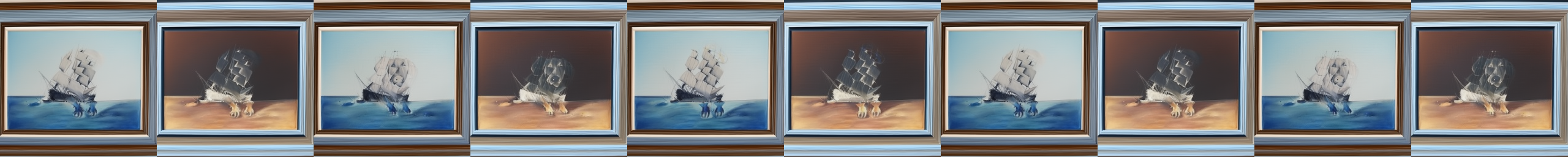
$1$-to-$n$ Projection, ‘‘an oil painting of {a watering can, a dragon}’’
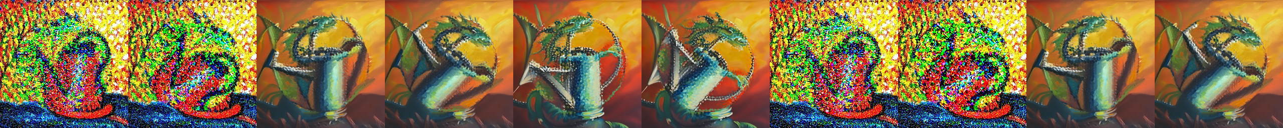
$n$-to-$1$ Projection, ‘‘a painting of {a car, an airplane}’’

Figure 3: Qualitative comparison of different joint denoising processes. While all cases perform well in the $1$-to-$1$ projections, Case 1, Case 3 and Case 4 exhibit degraded performance when a projection is $1$-to-$n$. Notably, SyncTweedies (Case 2) can be applied to the widest range of projections, including $n$-to-$1$ projections.

3.4 Comparison Across the Joint Diffusion Processes

Here, we compare the five cases of joint diffusion processes in Section 3.2 and analyze their characteristics through various toy experiments.

3.4.1 Toy Experiment Setup: Ambiguous Image Generation.

For the toy experiment setup, we employ the task of generating ambiguous images introduced by Geng et al.  [11] (see Section 3.3 for descriptions of ambiguous images). We consider two instance spaces: one is identical to the canonical space (with the identity transformation), and the other is a transformation of the canonical space, employing one of the 10 transformations used by Geng et al.  [11]: flips, rotations, color inversion, and pixel permutations; all of which are $1$-to-$1$ projections. In our experiments, we use DeepFloyd [9] as the pretrained image diffusion model, and the 95 prompt pairs introduced by Geng et al.  [11] were used for each type of transformation, resulting in a total of 950 generated ambiguous images.

The quantitative and qualitative results of the five cases of joint diffusion processes are presented in Table 1 and Figure 3. For detailed information on the evaluation, refer to the supplementary material. As illustrated, the results are similar across all joint diffusion processes, indicating that any of those can be chosen for this specific task.

3.4.2 $1$-to-$n$ Projection.

We further investigate the five cases of joint diffusion processes with different transformations for ambiguous images. It is important to note that all the transformations previously mentioned are perfectly invertible, meaning: $f_{i}(g_{i}(\mathbf{w}_{i}))=\mathbf{w}_{i}$. However, in certain applications, the projection $f_{i}$ is often not a function but an $1$-to-$n$ mapping, thus not allowing its inverse. For example, consider generating a texture image of a 3D object while treating the texture image space as the canonical space and the rendered image spaces as instance spaces. When mapping each pixel of a specific view image to a pixel in the texture image in the rendering process—with nearest neighbor sampling, one pixel in the texture space can be projected to multiple pixels. Hence, the unprojection operation $g_{i}$ cannot be a perfect inverse of the projection $f_{i}$ but can only be an approximation, making the reprojection error $\|\mathbf{w}_{i}-f_{i}(g_{i}(\mathbf{w}_{i}))\|$ small. We observe that such a case of having $1$-to-$n$ projection $f_{i}$ can significantly impact the joint diffusion process.

As a toy experiment setup illustrating such a case with ambiguous image generation, we use rotations with nearest-neighbor sampling as transformations. We randomly select an angle and rotate an inner circle of the image while leaving the rest of the region unchanged. Due to discretization, rotating an image followed by an inverse rotation may not perfectly restore the original image.

The second row of Table 1 and Figure 3 present the quantitative and qualitative results of this experiment. Note that the performance of Case 1 and Case 4, which aggregate the predicted noises $\boldsymbol{\epsilon}_{\theta}(\cdot)$ from either instance variables $\mathbf{w}_{i}^{(t)}$ or a projected canonical variable $f_{i}(\mathbf{z}^{(t)})$ respectively, significantly declines. Also, the performance of Case 3, which aggregates the posterior means $\psi_{\sigma_{t}}^{(t)}(\cdot,\cdot)$, shows a minor decline. Case 2 and Case 5, however, remain almost unchanged. This highlights that the denoising process is highly sensitive to the predicted noise and to the intermediate noisy data points, while it is much more robust to the outputs of Tweedie’s formula [39] $\phi^{(t)}(\cdot,\cdot)$, the prediction of the final clean data point at an intermediate stage.

3.4.3 $n$-to-$1$ Projection.

Then, do the results above conclude that both Case 2 and 5 are suitable for all applications? Lastly, we consider the case when the projection $f_{i}$ also involves an $n$-to-$1$ mapping. Such a scenario can arise when coloring not a solid mesh but a neural 3D representation rendered with the volume rendering equation [20, 21, 32]. Due to the nature of volume rendering, which involves sampling multiple points along a ray and taking a weighted average of their information, the projection operation $f_{i}$ includes an $n$-to-$1$ mapping. In this case, Case 5 results in poor outcomes due to a variance decrease issue. Let $\{\mathbf{x}_{i}\}_{i=1:N}$ be random variables, each sampled from $\mathbf{x}_{i}\sim\mathcal{N}(\boldsymbol{\mu}_{i},\sigma_{t}^{2}\mathbf{I})$, and $\mathbf{x}=\sum_{i=1}^{N}w_{i}\mathbf{x}_{i}$ be the weighted average, where $0\leq w_{i}\leq 1$ and $\sum_{i=1}^{N}w_{i}=1$. Then, $\mathbf{x}$ also follows the Gaussian distribution:

$$\mathbf{x}\sim\mathcal{N}\left(\sum_{i=1}^{N}w_{i}\boldsymbol{\mu}_{i},\sum_{i=1}^{N}w_{i}^{2}\sigma_{t}^{2}\mathbf{I}\right).$$ (9)

From the triangle inequality [33], the sum of squares is always less than or equal to the square of the sum: $\sum_{i=1}^{N}w_{i}^{2}\leq(\sum_{i=1}^{N}w_{i})^{2}=1$, implying that the variance of $\mathbf{x}$ is mostly less than the variance of $\mathbf{x}_{i}$. Consequently, when $f_{i}$ includes an $n$-to-$1$ mapping, the variance of $\mathbf{w}_{i}^{(t)}$, computed as a weighted average over multiple points in the canonical space, is less than the variance of $\mathbf{z}^{(t)}$. Thus, the final output of Case 5 becomes blurry and coarse since each intermediate noisy latent in instance spaces $\mathbf{w}_{i}^{(t)}$ experiences a decrease in variance compared to that of $\mathbf{z}^{(t)}$.

We validate our analysis with another toy experiment, where we use the same set of transformations used by Geng et al.  [11] but with a multiplane image (MPI) [45] as the canonical space. The image of each instance space is rendered by first averaging colors in the multiplane of the canonical space and then applying the transformation. Three planes are used for the multiplane image representation in our experiments. The results are presented in the third row of Table 1 and Figure 3. Notably, Case 5 also produces blurry images like the other cases, whereas Case 2 still generates realistic images.

Table 2 below summarizes suitable cases for each projection type. Note that Case 2, which has not been attempted in any of the previous works, is the only case that is applicable to any type of projection function. Since Case 2 involves averaging the outputs of Tweedie’s formula in the instance spaces, we name this case SyncTweedies. Experimental results with additional applications are also demonstrated in Section 5.

Projection	Case 1	Case 2 SyncTweedies	Case 3	Case 4	Case 5
$1$-to-$1$	✔	✔	✔	✔	✔
$1$-to-$n$	✗	✔	✗	✗	✔
$n$-to-$1$	✗	✔	✗	✗	✗

Table 2: Analysis of joint diffusion processes on projection operations. SyncTweedies (Case 2) offers the broadest range of applications.

4 Related Work

In addition to Section 3.3 introducing previous works on joint diffusion, in this section, we review other previous works that utilize pretrained image diffusion models in different ways to generate or edit visual content.

4.1 Optimization-Based Methods

Poole et al. [35] first introduced Score Distillation Sampling (SDS) technique, which facilitates data sampling in a canonical space by leveraging the loss function of the diffusion model training and conducting gradient descent in each instance space. This idea, originally introduced for 3D generation [46, 26, 44], has been widely applied to various applications, including vector image generation [19], ambiguous image generation [6], mesh texturing [48], mesh deformation [47], and 4D generation [27, 3]. Subsequent works [14, 22, 23] also proposed modified loss functions not to generate data but to edit existing data while preserving their identities. This approach, exploiting diffusion models not for denoising but for gradient-descent-based iterative updating, generally produces less realistic outcomes compared to denoising-based generation results, while also taking much more time.

4.2 Iterative View Updating Methods

Particularly for 3D object/scene texturing and editing, there are approaches to iteratively update each view image and subsequently update the 3D object/scene. TEXTure [38], Text2Tex [8], and TexFusion [7] are previous works that repeatedly generate a projective texture from each view and unproject it onto the 3D mesh for texture updating. Notably for NeRF editing, Instruct-NeRF2NeRF [13] proposed to edit a NeRF scene by iteratively replacing each view image used in the NeRF optimization and then updating the NeRF model. However, sequentially updating the canonical sample leads to error accumulations, resulting in blurriness or inconsistency across different views.

In Section 5.2 and 5.3, we compare our synchronized joint diffusion processes with the aforementioned techniques in 3D mesh and 3D Gaussian splat texturing, demonstrating the superior quality of joint diffusion processes with fast computational speed.

5 Applications

In this section, we present quantitative and qualitative results of different joint diffusion processes on various applications, including depth-to-360-panorama generation (Section 5.1), 3D mesh texturing (Section 5.2) and 3D Gaussian splat [21] texturing (Section 5.3). Following the toy experiments described in Section 3.4.1, we compare the five cases of joint diffusion processes introduced in Section 3.2, along with optimization-based methods and iterative-update-based methods introduced in Section 4.

Refer to Section 3.3 for the detailed definition of the canonical space $\mathcal{Z}$, the instance spaces $\{\mathcal{W}_{i}\}_{i=1:N}$, the projection operation $f_{i}$, and the unprojection operation $g_{i}$ in each application. Please refer to the supplementary material for additional detailed experiments and more comprehensive experiment setups, including: (1) $360^{\circ}$ rendering videos of textured 3D meshes and 3D Gaussian splats, (2) results of orthographic panorama generation, (3) a comparison of computation times, and (4) implementation details of each application.

5.0.1 Evaluation Setup.

Across all the following applications, we compute FID [15], KID [5] and GIQA [12] to assess the fidelity of the generated images. Additionally, we measure CLIP similarity [36] (CLIP-S) to evaluate conformity to the input text prompt. We use a depth-conditioned ControlNet [49] as the pretrained image diffusion model.

Metric Case 1 Case 2 Sync- Tweedies Case 3 Case 4 Case 5 FID [15] $\downarrow$ 364.61 42.11 55.95 348.18 43.39 KID [5] $\downarrow$ 375.42 21.19 34.67 362.77 22.87 GIQA [12] $\uparrow$ 18.16 24.25 23.85 18.93 24.12 CLIP-S [36] $\uparrow$ 19.75 28.01 27.19 19.93 27.99

Table 3: A quantitative comparison in a Depth-to-360-Panorama application. KID and GIQA are scaled by $10^{3}$ and $10^{4}$, respectively. The best in each row is highlighted by bold.

	‘‘an old looking library’’	‘‘a house at night’’
Input Depth
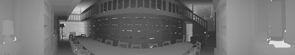
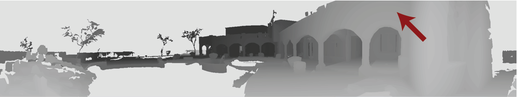
Case 1
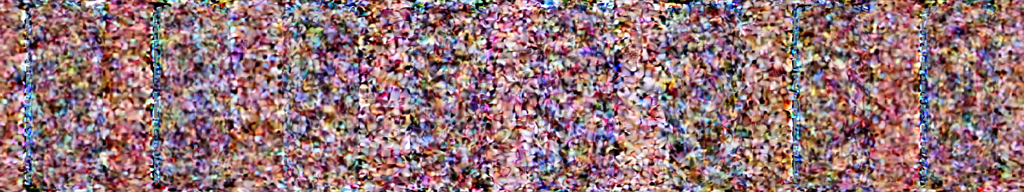
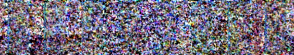
Case 2 Synctweedies
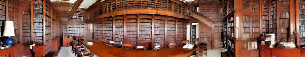
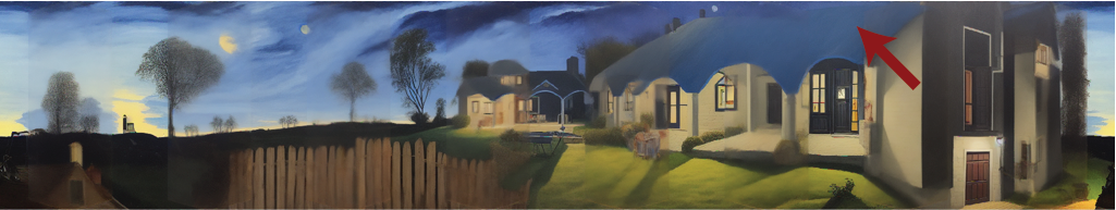
Case 3
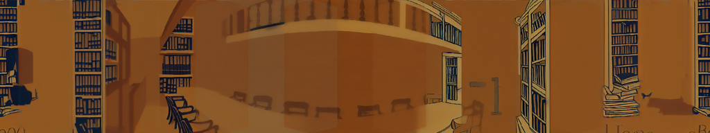
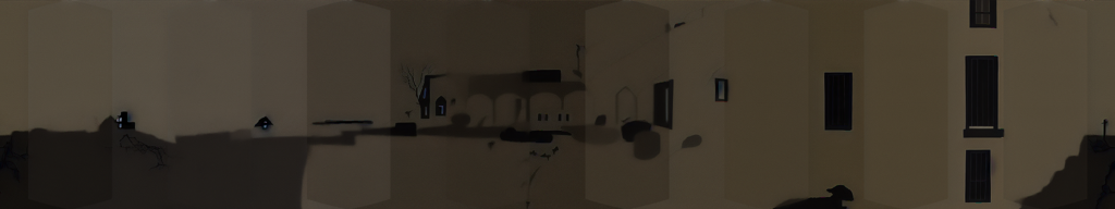
Case 4
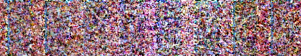
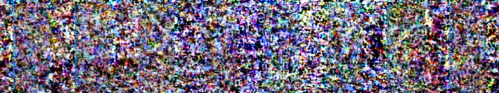
Case 5

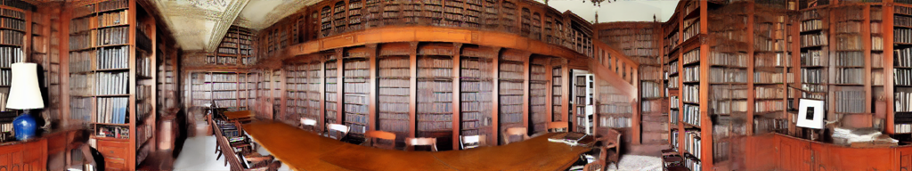
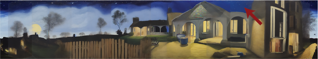
Figure 4: Qualitative results of $360^{\circ}$ panorama generation. SyncTweedies (Case 2) and Case 5 generate consistent and high-fidelity $360^{\circ}$ panorama images as observed in the $1$-to-$n$ projection experiment in Section 3.4.2. Case 1 and Case 4 fail to generate meaningful $360^{\circ}$ panorama images, while Case 3 tends to lose details.

5.1 Depth-to-360-Panorama

We generate $360^{\circ}$ panorama images from input $360^{\circ}$ depth maps obtained from 360MonoDepth [37] dataset. Here, the projection operation $f_{i}$ is a perspective transformation from the $360^{\circ}$ panorama canvas to a perspective view image, which is an $1$-to-$n$ projection due to the discretization. We generate a total of 1,000 $360^{\circ}$ panorama images at 0^∘ elevation, and a field of view of $72^{\circ}$.

5.1.1 Results.

We report quantitative and qualitative results of the five joint diffusion processes discussed in Section 3.2 in Table 3 and Figure 4, respectively. Table 3 demonstrates a trend consistent with the $1$-to-$n$ projection toy experiment results shown in Section 3.4.1. Specifically, SyncTweedies (Case 2) and Case 5, which synchronize the outputs of Tweedie’s formula $\phi^{(t)}(\cdot,\cdot)$, exhibit the best performance. Notably, SyncTweedies (Case 2) demonstrates slightly superior performance across all metrics. In Figure 4, we observe that Case 1 and Case 4, which aggregate the predicted noise $\boldsymbol{\epsilon}_{\theta}(\cdot)$, produce noisy outputs. Case 3 yields suboptimal $360^{\circ}$ panorama images, characterized by a monochromatic appearance and lack of details. SyncTweedies (Case 2) and Case 5 demonstrate the best results aligning with the input depth image, with SyncTweedies (Case 2) showing a slightly better alignment as indicated by the red arrow in Figure 4.

Table 4: A quantitative comparison in a 3D mesh texturing application. KID and GIQA are scaled by $10^{3}$ and $10^{4}$, respectively. The best in each row is highlighted by bold.

Metric	Joint Diffusion					Optim. -Based	Iter. View Updating
	Case 1	Case 2 SyncTweedies	Case 3	Case 4	Case 5	Paint-it [48]	TEXTure [38]	Text2Tex [8]
FID [15] $\downarrow$	135.61	21.76	36.12	131.67	22.76	28.23	34.98	26.10
KID [5] $\downarrow$	68.63	1.46	6.60	65.70	1.74	2.30	6.83	2.51
GIQA [12] $\uparrow$	21.13	34.91	30.18	21.20	34.07	31.50	28.91	31.43
CLIP-S [36] $\uparrow$	25.26	28.89	27.88	25.31	28.82	28.55	28.63	27.94

Prompt	Joint Diffusion					Optim. -Based	Iter. View Updating
	Case 1	Case 2 Sync- Tweedies	Case 3	Case 4	Case 5	Paint-it [48]	TEXTure [38]	Text2Tex [8]

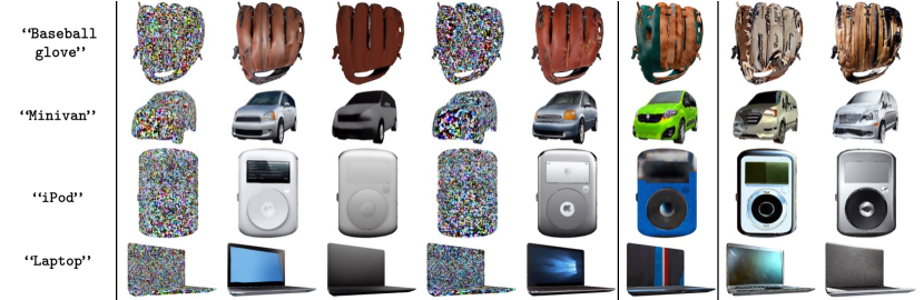
Figure 5: 3D mesh texturing qualitative result. SyncTweedies (Case 2) and Case 5 exhibit comparable results, outperforming other baselines. The optimization-based method shows view inconsistency, while iterative-update-based methods generates images without fine details.

5.2 3D Mesh Texturing

In 3D mesh texturing, projection operation $f_{i}$ is a rendering function which outputs perspective view images from a 3D mesh with a texture image. This operation represents a 1-to-n projection due to discretization. We evaluate five joint diffusion cases along with Paint-it [48], an optimization-based method, and TEXTure [38] and Text2Tex [8], which are iterative-update-based methods. This evaluation is conducted on a dataset comprising 429 mesh and prompt pairs collected from TEXTure [38] and Text2Tex [8].

5.2.1 Results.

We present quantitative and qualitative results in Table 4 and Figure 5, respectively. The results in Table 4 align with the observations made in the $1$-to-$n$ projection case discussed in Section 3.4.2. Quantitatively, SyncTweedies (Case 2) and Case 5 outperform other baselines across all metrics, but our proposed method demonstrates superior performance compared to Case 5. Notably, our method shows superior performance to optimization-based and iterative-update-based methods.

In Figure 5, SyncTweedies (Case 2) and Case 5 generate most realistic output images. The optimization-based method [48] shows inconsistencies across views, as evidenced by artifacts such as fragmented fingers on baseball gloves in row 1 and distorted front bumpers of a car in row 2. The iterative-update-based methods [38, 8] produce blurry images lacking fine details, noticeable in the screens of the iPod and the laptop in rows 3 and 4, respectively.

Metric	Joint Diffusion		Optim. Based	Iter. View. Updating
	Case 2 Sync- Tweedies	Case 5	SDS [35]	IN2N [13]
FID [15] $\downarrow$	100.13	108.99	119.56	109.65
KID [5] $\downarrow$	13.67	15.36	22.78	15.73
GIQA [12] $\uparrow$	27.87	26.16	25.72	26.98
CLIP-S [36] $\uparrow$	29.44	28.92	30.15	29.25

Table 5: A quantitative comparison of texturing 3D Gaussian splats. KID and GIQA are scaled by $10^{3}$ and $10^{4}$, respectively. The best in each row is highlighted by bold.

Figure 6: Qualitative results of texturing 3D Gaussian splats. Case 5 tends to lose details due to the variance decrease issue, whereas SyncTweedies (Case 2) generates realistic images by avoiding this issue. The optimization-based method [35] produces high-contrast, colors and the iterative view updating method [13] yields suboptimal outputs due to error accumulation.

Prompt	Ground Truth	Joint Diffusion		Optim.-Based	Iter. View. Updating
		Case 2 SyncTweedies	Case 5	SDS [35]	IN2N [13]
‘‘A tree with multicolored leaves’’
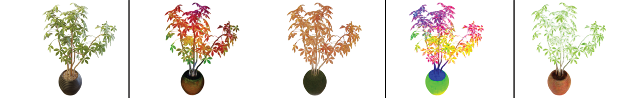
‘‘Wooden carving of a microphone’’
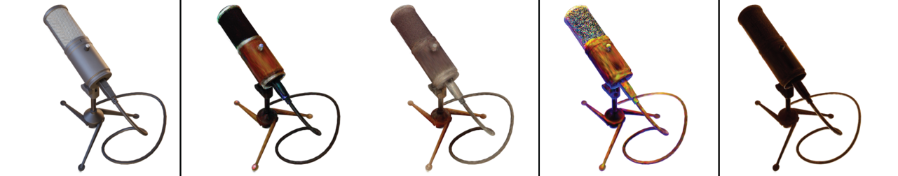
‘‘Wooden carving of a ship’’

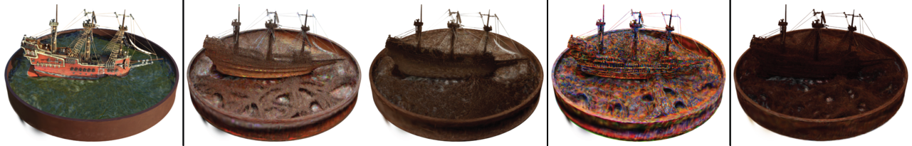
5.3 3D Gaussian Splat Texturing

Lastly, to verify the difference between Case 2 (SyncTweedies) and Case 5, both of which demonstrate applicability up to $1$-to-$n$ projections as outlined in Section 3.4.1, we explore texturing 3D Gaussian splats [21], exemplifying an $n$-to-$1$ projection case. In 3D Gaussian splats texturing, the projection operation $f_{i}$ is an $n$-to-$1$ case, characterized by a volumetric rendering function [20]. This function computes a weighted sum of $n$ 3D Gaussians splats in the canonical space to render a pixel in the instance space.

While recent 3D generative models [44, 43] generate plausible 3D objects represented as 3D Gaussian splats, they often lack fine details in the appearance. We validate the effectiveness of SyncTweedies (Case 2) on pretrained 3D Gaussian splats [21] trained on multi-view images from the Synthetic NeRF dataset [32]. We use 50 views for texture generation and evaluate the results from 150 unseen views. For baselines, we evaluate SyncTweedies (Case 2) with Case 5, the optimization-based method SDS [35], and the iterative-update-based method Instruct-NeRF2NeRF (IN2N) [13]. We only include SyncTweedies (Case 2) and Case 5 from joint diffusion processes since they are shown to be the most robust cases against different projections as discussed in Section 3.4.1.

5.3.1 Results.

Table 5 presents a quantitative comparison of 3D Gaussian splat [21] texturing, and Figure 6 shows qualitative results. SyncTweedies (Case 2), unaffected by the variance decrease issue, outperforms Case 5, as observed in the toy experiments in Section 3.4.1. When compared to other baselines based on optimization (SDS [35]) and iterative view updating (IN2N [13]), our method outperforms across most metrics, especially by a large margin in FID [15].

Figure 6 demonstrates that SyncTweedies (Case 2) generates high-fidelity results with intricate details, such as the colorful leaves of the tree in row 1, while Case 5 produces monochromatic images. SDS [35] results in artifacts characterized by high saturation as the body of the microphone in row 2. IN2N [13] fails to preserve fine details, such as the carvings of a ship in row 3.

6 Conclusion and Future Work

We have explored various scenarios for synchronizing multiple denoising processes and evaluated their performance across a range of applications, including ambiguous image generation, panorama generation, 3D mesh texturing, and 3D Gaussian splats texturing. Through this investigation, we have demonstrated that the approach named SyncTweedies, which averages the outputs of Tweedie’s formula while conducting denoising in multiple instance spaces, offers the best performance and widest applicability.

Despite the best performance of SyncTweedies across the synchronization cases, averaging the outputs of Tweedie’s formula may still lead to performance degradation. This limitation could be addressed by fine-tuning a model on a small scale dataset. Furthermore, we aim to delve deeper into the potential of synchronized denoising processes across a broader spectrum of applications with data modalities such as audio, video, human motions, and others.

Appendix

A1 Experiment Details

In this section, we provide details of the experiments discussed . For all joint denoising processes, we use a fully deterministic DDIM [42] sampling with 30 steps. In the case of instance variable denoising processes introduced in Section 3.2  (Cases 1 to Case 3), we initialize instance variables by projecting an initial canonical latent $\mathbf{z}^{(T)}$ sampled from a unit Gaussian distribution $\mathcal{N}(\mathbf{0},\mathbf{I})$: $\mathbf{w}_{i}^{(T)}\leftarrow f_{i}(\mathbf{z}^{(T)})$. For $n$-to-$1$ projection cases, the instance variables are directly initialized from a unit Gaussian distribution to avoid the variance decrease issue discussed in Section 3.4.1 .

As described in Section 3.4.1 and Section 5 , we use DeepFloyd [9] as the pretrained diffusion model for the ambiguous image generation which denoises images in the RGB space. For the depth-to-360-panorama generation, 3D mesh texturing, and 3D Gaussian splat texturing, we employ a pretrained depth-conditioned ControlNet [49] which is based on a latent diffusion model, specifically Stable Diffusion [40]. For applications utilizing ControlNet, synchronization during the intermediate steps of joint denoising processes occurs within the same latent space, except for 3D Gaussian splat texturing. In the case of 3D Gaussian splat texturing, synchronization takes place in the RGB space, and detailed explanations are provided in Section A1.4.

At the end of the joint denoising processes, we perform the final synchronization in the RGB space using the decoded instance variables across all applications.

A1.0.1 Evaluation Metrics.

For all applications, we evaluate diversity and fidelity of the generated images using FID [15] and KID [5]. Additionally, we measure GIQA [12] to assess the fidelity of individual generated images. These metrics compute scores based on the distance between the distribution of the generated image set and that of the reference image set, with the reference set forming the target distribution. Refer to each application section for detailed description of constructing the generated image set and the reference image set.

To evaluate the text alignment of the generated images, we report CLIP similarity score [36] (CLIP-S) which measures the similarity between the generated images $\mathbf{w}^{(0)}_{i}$ and their corresponding text prompts $p_{i}$ in CLIP [36] embedding space. Additionally, in the ambiguous image generation, we report CLIP alignment score (CLIP-A) and CLIP concealment score (CLIP-C) following previous work, Visual Anagrams [11]. To compute the metrics, we begin by calculating a CLIP similarity matrix $\mathbf{S}\in\mathbb{R}^{N\times N}$ from $N$ pairs of transformations and text prompts:

$$\mathbf{S}_{ij}=E_{\text{img}}(f_{i}(\mathbf{z}^{(0)}))^{T}E_{\text{text}}(p_{j}),$$ (10)

where $E_{\text{img}}(\cdot)$ and $E_{\text{text}}(\cdot)$ are the image encoder and the text encoder of the pretrained CLIP model [36], respectively. CLIP-A quantifies the worst alignment among the corresponding image-text pairs, specifically computed as $\min\text{diag}(\mathbf{S})$. However, this metric does not account for misalignment failure cases, where $p_{i}$ is visualized in $\mathbf{w}^{(0)}_{j}$ for $i\neq j$. CLIP-C considers alignment of an (a) image (prompt) to all prompts (images) by normalizing the similarity matrix $\mathbf{S}$ with a softmax operation:

$$\frac{1}{N}\text{tr}(\text{softmax}(\mathbf{S}/\tau)),$$ (11)

where $\text{tr}(\cdot)$ denotes the trace operator, and $\tau=0.07$ is the temperature parameter of CLIP [36].

A1.1 Details on Ambigous Image Generation — Section 3.4.1

We present the details of the ambiguous image generation experiments in Section 3.4.1 . Quantitative and qualitative results are presented in Table 1 and Figure 3 .

A1.1.1 Evaluation Setup.

To evaluate the fidelity of the generated images using FID, KID, and GIQA, we create a reference set consisting of 5,000 generated images from Stable Diffusion 1.5 [40] with the same text prompts used in the generation of ambiguous images.

A1.1.2 Implementation Details

We use DeepFloyd [9] which is a two-stage cascaded diffusion model. In the first stage, we generate $64\times 64$ images that are upscaled to $256\times 256$ images in the subsequent stage.

A1.1.3 Definition of Operations.

In the context of ambiguous image generation, both the instance variables $\{\mathbf{w}_{i}\}_{i=1:N}$ and canonical variables $\mathbf{z}$ share the same image space. However, instance variables exhibit different appearances from the canonical variable upon applying certain transformations.

In the $1$-to-$1$ projection case, we use the 10 transformations used in Visual Anagrams [11], all of which are $1$-to-$1$ mappings. The projection operation $f_{i}$ is defined as the transformation itself, and the unprojection operation $g_{i}$ is defined as the inverse of the transformation matrix.

In the scenario of $1$-to-$n$ projection, we employ inner circle rotation as the projection operation $f_{i}$. This involves rotating the pixels within an inner circle of an image while keeping the outer pixels unchanged. The unprojection operation $g_{i}$ is the inverse of $f_{i}$. We use $14$ inner circle rotation transformations, with rotation angles evenly spaced in the range $[45^{\circ},175^{\circ}]$. For evaluation, we utilize the same 95 prompts as in the $1$-to-$1$ case for each transformation, generating $14\times 95=1,350$ ambiguous images. After applying a rotation transformation, the grid of the rotated image does not align with the original image grid. Thus, we use the nearest-neighbor sampling to retrieve pixel colors from the original image to the rotated image. This sampling process leads to a scenario where a single pixel in the original image $\mathbf{z}$ can be mapped to multiple pixels in the rotated image $\mathbf{w}_{i}$, which is a $1$-to-$n$ mapping.

For $n$-to-$1$ projection, we use the same transformations and text prompts as in the $1$-to-$1$ projection experiment, thus resulting in a total of $10\times 95=950$ ambiguous images. The only difference from the $1$-to-$1$ projection experiment is that the canonical space variable $\mathbf{z}$ is now represented as multiplane images (MPI) [45], where a collection of planes $\{\mathbf{p}_{j}\}_{j=1:M}$ represents a single canonical variable. Specifically, we compute $\mathbf{z}$ by averaging the multiplane images: $\mathbf{z}=\frac{1}{M}\sum_{j=1}^{M}\mathbf{p}_{j}$. In the context of $n$-to-$1$ projection, we substitute the sequence of the unprojection $g_{i}$ and the aggregation $\mathcal{A}$ operation with an optimization process. The multiplane images ${\mathbf{p}_{j}}$ are optimized using the following objective function:

$$\min_{\{\mathbf{p}_{j}\}}\sum_{i}^{N}\left|f_{i}\left(\frac{1}{M}\sum_{j=1}^{M}\mathbf{p}_{j}\right)-\mathbf{w}_{i}\right|,$$ (12)

where the number of planes $M=3$ .

A1.2 Details on Depth-to-360-Panorama Generation — Section 5.1

We provide details of the Depth-to-360-Panorama generation experiments presented in Section 5.1 . Refer to Table 3 and Figure 4  for quantitative and qualitative results.

A1.2.1 Evaluation Setup.

We evaluate SyncTweedies and the baseline methods on 1,000 pairs of $360^{\circ}$ panorama images and depth maps randomly sampled from 360MonoDepth [37] dataset. For each $360^{\circ}$ panorama image, we generate a text prompt using the output of BLIP [25] by providing a perspective view image of the panorama as input.

In the $360^{\circ}$ panorama generation, we use eight perspective views by evenly sampling azimuths with $45^{\circ}$ intervals at $0^{\circ}$ elevation. Each perspective view has a field of view of $72^{\circ}$. For evaluation, we project the generated $360^{\circ}$ panorama image to ten perspective views with randomly sampled azimuths at $0^{\circ}$ elevation and a field of view of $60^{\circ}$. Similarly, the reference set images are obtained by projecting each ground truth $360^{\circ}$ panorama image into ten perspective views with azimuths randomly sampled and at $0^{\circ}$ elevation. In total, we use $1,000\times 10=10,000$ perspective view images for evaluation.

A1.2.2 Implementation Details.

We set the resolution of a latent panorama image to 2,048 $\times$ 4,096 and that of the latent perspective view images to 64 $\times$ 64. In the RGB space, a panorama image has a resolution of 1,024 $\times$ 2,048, and perspective view images have a resolution of 512 $\times$ 512.

We adopt two approaches introduced in SyncMVD [29], Voronoi-diagram-based filling [2] and modified self-attention layers. First, the high resolution of the latent panorama image results in panorama images with sparse pixel distribution. To address this issue, we propagate the unprojected pixels to the visible regions of the panorama using the Voronoi-diagram-based filling. Second, spatially distant views tend to generate inconsistent outputs. Therefore, we adopt the modified self-attention mechanism that attends to other views when computing the attention output.

A1.2.3 Definition of Operations.

In the $360^{\circ}$ panorama generation, the canonical variable $\mathbf{z}$ represents a $360^{\circ}$ panorama image, while the instance variables $\{\mathbf{w}_{i}\}_{i=1:N}$ correspond to perspective views of the panorama. The mappings between the panorama image and the perspective views are computed as follows: First, we unproject the pixels of the perspective view image to the 3D space. Then, we apply two rotation matrices based on the azimuth and elevation angles. The pixels are then reprojected onto the surface of a unit sphere, represented as longitudes and latitudes. These spherical coordinates are finally converted to 2D coordinates on the panorama image.

Given the mappings, the projection operation $f_{i}$ samples colors from the panorama image using the nearest-neighbor method. Since a single pixel of a panorama image $\mathbf{z}$ can be mapped to multiple pixels of a perspective view image $\mathbf{w}_{i}$, the $360^{\circ}$ panorama generation is a $1$-to-$n$ projection case, as discussed in Section 3.4.2 .

A1.3 Details on 3D Mesh Texturing — Section 5.2

We provide details of the 3D mesh texturing experiments presented in Section 5.2 . Quantitative and qualitative results are shown in Table 4 and Figure 5 .

A1.3.1 Evaluation Setup.

We use 429 mesh and prompt pairs collected from previous works, TEXTure [38] and Text2Tex [8]. For texture generation, we use eight views sampled around the object with $45^{\circ}$ intervals at $0^{\circ}$ elevation. Two additional views are sampled at $0^{\circ}$ and $180^{\circ}$ azimuths with $30^{\circ}$ elevation. For evaluation, we render a 3D mesh to ten perspective views with randomly sampled azimuths at $0^{\circ}$ elevation, resulting $10\times 429=$ 4,290 images. Following SyncMVD [29], the reference set images are generated by ControlNet [49] using the same depth maps and text prompts used in the texture generation.

A1.3.2 Implementation Details.

As done in the $360^{\circ}$ panorama generation, we apply the Voronoi-diagram-based filling after each unprojection operation and employ the modified self-attention mechanism. The resolution of the latent texture image is $1,536\times 1,536$, and that of the latent perspective view images is $96\times 96$. In the RGB space, the resolution of the texture image is $1,024\times 1,024$ and that of the perspective view images is $768\times 768$.

A1.3.3 Definition of Operations.

In the 3D mesh texturing, the canonical variable $\mathbf{z}$ is the texture image of a 3D mesh, and the instance variables $\{\mathbf{w}_{i}\}_{i=1:N}$ are rendered images from the 3D mesh. The projection operation $f_{i}$ is a rendering function where nearest-neighbor sampling is utilized to retrieve the color from the texture image to perspective view images.

As done in the $n$-to-$1$ projection case in Section A1.1, we replace the unprojection $g_{i}$ and aggregation $\mathcal{A}$ operation to an optimization process. This process optimizes the texture image $\mathbf{z}$ using the multi-view images ${{\mathbf{w}i}}{i=1:N}$. In the 3D mesh texturing, one pixel in the texture image $\mathbf{z}$ can be mapped to multiple pixels in a rendered image $\mathbf{w}_{i}$. Hence, this application corresponds to the $1$-to-$n$ projection case as in Section 3.4.2 .

A1.4 Details on 3D Gaussian Splat Texturing — Section 5.3

We provide details of the 3D Gaussian splat texturing experiment presented in Section 5.3. Quantitative and qualitative results are provided in Table 5 and Figure 6 .

A1.4.1 Evaluation Setup.

For evaluation, we use pretrained 3D Gaussian splats trained with multi-view images from the Synthetic NeRF dataset [32], consisting of 8 objects. We generate 40 textured 3D Gaussian splats by utilizing five different prompts per 3D object. We use 50 views for texture generation and 150 unseen views for evaluation.

A1.4.2 Implementation Details.

As described in Section A1, we employ ControlNet [49] which denoises latent images. To render the latent images, we replace the spherical harmonics coefficients of a 3D Gaussian splat to a 4-channel latent vector.

Additionally, we empirically observe that 3D Gaussian splats optimized in the RGB space yield better results than those optimized in the latent space. Hence, SyncTweedies optimizes 3D Gaussian splats in the RGB space by decoding the outputs of the Tweedie’s formula. However, this approach cannot be extended to other cases that i) do not synchronize the outputs of $\phi(\cdot,\cdot)$ and ii) compute $\psi(\cdot,\cdot)$ in the canonical space. For this reason, we optimize 3D Gaussian splats in the latent space for Case 5.

A1.4.3 Definition of Operations.

The canonical variables $\{\mathbf{z}_{j}\}_{j=1:M}$ are 3D Gaussian splats and the instance space variables $\{\mathbf{w}_{i}\}_{i=1:N}$ are the rendered images from the 3D Gaussian splats. The projection operation $f_{i}$ is a volume rendering function [20, 21] where the colors (latent vectors) of multiple 3D Gaussian splats are composited to render a pixel. This corresponds to the $n$-to-$1$ projection as discussed in Section 3.4.3. In 3D Gaussian splat texturing, the colors of 3D Gaussian splats $\mathbf{z}=\{\mathbf{s}_{j}\}_{j=1:M}$ are optimized from multi-view images $\{\mathbf{w}_{i}\}_{i=1:N}$ as in the $n$-to-$1$ experiment in Section 3.4.3 .

A2 Orthographic Panorama Generation

In addition to the $1$-to-$1$ projection case presented in Section 3.4.1, we present orthographic panorama generation. In contrast to the $360^{\circ}$ panorama generation which corresponds to the $1$-to-$n$ projection case, orthographic panorama generation involves $1$-to-$1$ projection.

A2.0.1 Evaluation Setup.

In orthographic panorama generation, we use Stable Diffusion 2.0 [40] as the pretrained diffusion model. We evaluate the five joint diffusion cases discussed in Section 3.2, Case 1 to Case 5, using the six text prompts collected from SyncDiffusion [24]. For quantitative evaluation, we report the four metrics used in the main paper: FID [15], KID [5], GIQA [12], and CLIP-S [36].

Following SyncDiffusion [24], we generate 500 panorama images per prompt with $512\times 3,072$ resolution, resulting in $500\times 6=3,000$ panorama images. For evaluation, we randomly crop a partial view of the panorama image with $512\times 512$ resolution. Similarly, $3,000$ reference images with $512\times 512$ resolution are generated from the pretrained diffusion model using the same text prompts.

A2.0.2 Implementation Details.

Following SyncDiffusion [24], we use a deterministic DDIM [42] sampler with 50 denoising steps. The resolution of the latent panorama image is $64\times 384$ and that of the latent images is $64\times 64$. The final panorama image has a resolution of $512\times 3,072$, and each cropped image has a resolution of $512\times 512$.

A2.0.3 Definition of Operations.

While both the $360^{\circ}$ panorama generation described in Section 5.1  and orthographic panorama generation involve the merging of multiple window images, orthographic panorama generation does not account for perspective projection. Instead, it crops a partial view of the panorama image without considering the perspective distortion.

Note that the grid of the panorama image $\mathbf{z}$ and the window images $\{\mathbf{w}_{i}\}_{i=1:N}$ are perfectly aligned. Hence, this corresponds to the $1$-to-$1$ projection case discussed in Section 3.4.1 of the main paper.

A2.0.4 Result.

We report quantitative results in Table A6 and qualitative results in Figure A7. The quantitative results align with the observations shown in the $1$-to-$1$ experiment in Section 3.4.1 , where all cases show comparable performances. This is further supported by the results in Figure A7, where all cases exhibit similar panorama images, suggesting that any of the options can be used when the projection is $1$-to-$1$.

Table A6: A quantitative comparison of orthographic projection panorama. KID and GIQA are scaled by $10^{3}$. For each row, we highlight the column whose value is within 95% of the best.

Metric	Case 1	Case 2 SyncTweedies	Case 3	Case 4	Case 5
FID [15] $\downarrow$	32.83	32.82	32.83	32.82	32.83
KID [5] $\downarrow$	7.79	7.79	7.79	7.79	7.80
GIQA [12] $\uparrow$	28.40	28.40	28.40	28.41	28.40
CLIP-S [36] $\uparrow$	31.69	31.69	31.69	31.69	31.69

	‘‘A photo of a city skyline at night’’
Case 1
Case 2 SyncTweedies
Case 3
Case 4
Case 5
	‘‘A photo of a forest with a misty fog’’
Case 1
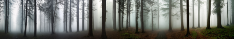
Case 2 SyncTweedies
Case 3
Case 4
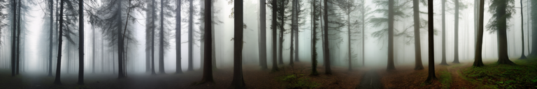
Case 5

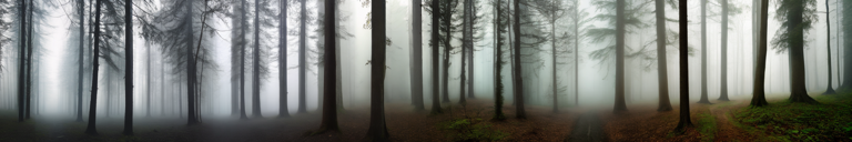
Figure A7: Qualitative results of orthographic projection panorama generation. All baselines show comparable results in the $1$-to-$1$ projection.

Generated 3D mesh [1]	Edited 3D mesh (SyncTweedies)
‘‘A nascar’’	‘‘A car with graffiti’’
‘‘A lantern’’	‘‘A Chinese style lantern’’
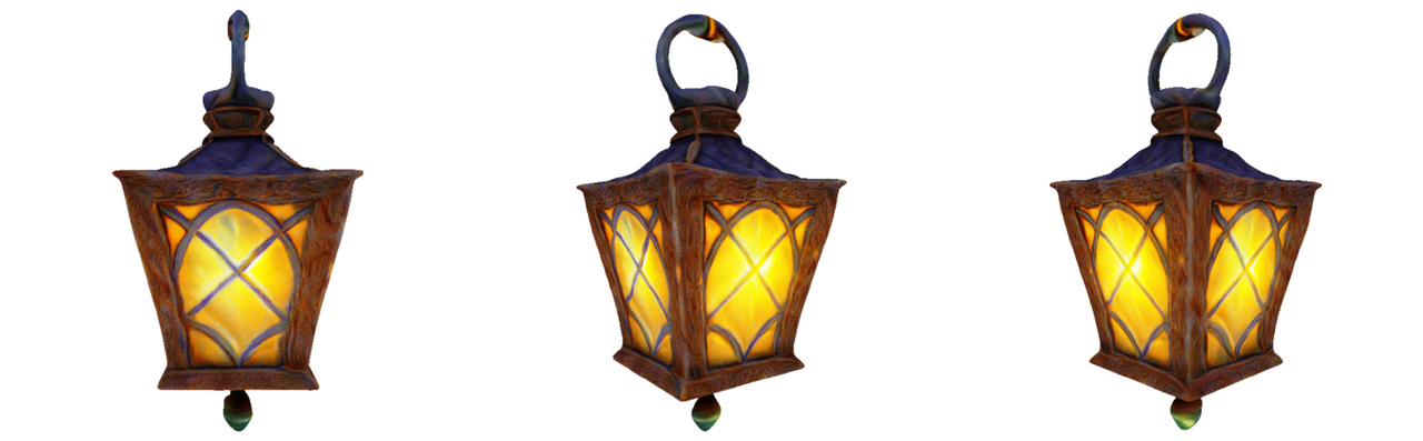
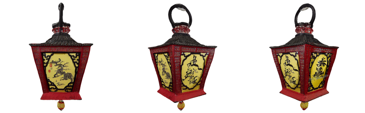
‘‘A turtle’’	‘‘A golden statue of a turtle’’

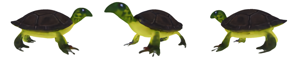
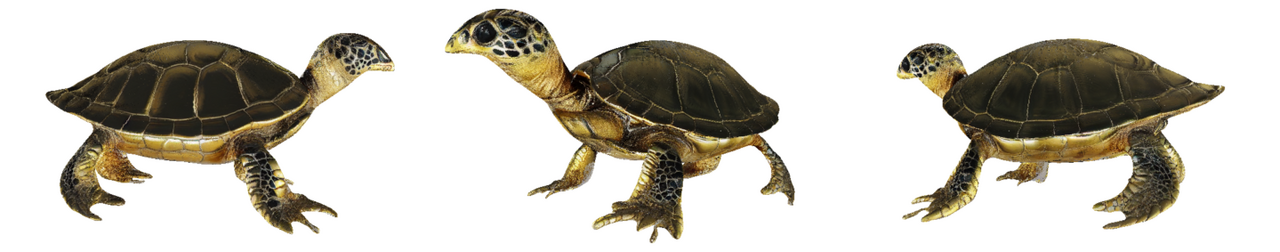
Figure A8: Qualitative results of 3D mesh texture editing. We edit the textures of the 3D meshes generated from Genies [1] using SyncTweedies.

A3 3D Mesh Texture Editing

In this section, we extend the 3D mesh texture generation in Section 5.2, and present texture editing application.

Despite the recent successes of 3D generation models [1, 28], the textures of the generated 3D meshes often lack fine details. We utilize SyncTweedies to edit the textures of the generated 3D meshes, and enhance the texture quality. Specifically, we use the 3D meshes generated from a text-to-3D model, Genie [1].

We follow SDEdit [30] to edit the textures of the 3D mesh. We begin by adding noise at intermediate time $t^{\prime}$ to the texture image of the 3D mesh, and take a reverse process starting from the same intermediate time $t^{\prime}$.

A3.0.1 Implementation Details.

We set the CFG weight [17] to $30$ and $t^{\prime}$ to $0.8$. For other settings, we follow the 3D mesh texture generation experiment presented in Section 5.2 .

A3.0.2 Results.

We present qualitative results of 3D mesh texture editing in Figure A8. The 3D meshes edited with SyncTweedies exhibit fine details, including graffiti on the car in row 1, paintings on the lantern in row 2, and the intricate shells of the turtle in row 3.

A4 Runtime Comparison

Table A7: A runtime comparison in 3D mesh texturing and 3D Gaussian splat texturing applications. The best in each row is highlighted by bold.

Metric	Joint Diffusion	Optim. -Based	Iter. View Updating
Runtime (minutes) $\downarrow$	3D Mesh Texturing
	Case 2 SyncTweedies	Paint-it [48]	TEXTure [38]	Text2Tex [8]
	1.83	21.95	1.54	13.10
	3D Gaussian Splats Texturing
	Case 2 SyncTweedies	SDS [35]	IN2N [13]
	10.56	85.50	37.93

As discussed in Section 4 , one of the advantages of joint diffusion processes is the fast computational speed. We compare the runtime performance of SyncTweedies with optimization-based and iterative-update-based methods in the 3D mesh texturing and the 3D Gaussian splat texturing. The quantitative results are presented in Table A7.

In the 3D mesh texturing, SyncTweedies shows faster computation times than other baselines except TEXTure [38] which shows comparable running time. However, TEXTure [38] generates suboptimal texture outputs as observed in Table 4 and Figure 5 . While another iterative-update-based method, Text2Tex [8], improves quality of texture image by integrating an additional refinement module, it introduces additional overhead in terms of running times. In contrast, SyncTweedies achieves running times that are 7 times faster than Text2Tex and even outperforms across all metrics as shown in Table 4 . Lastly, SyncTweedies shows 11 times faster running time when compared to Paint-it [48], an optimization-based method.

In the 3D Gaussian splats texturing, SyncTweedies achieves the fastest running time. SyncTweedies is 3 times faster than the iterative-update-based method IN2N [13], and 8 times faster than the optimization-based method, SDS [35]. This shows that SyncTweedies not only generates high-fidelity textures, but also excels other baselines in computational speed.

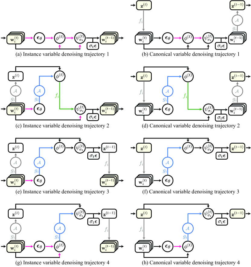
Figure A9: Diagrams of joint diffusion processes. All feasible trajectories of the instance variable denoising process (left) and the canonical variable denoising process (right). Each row shares the same trajectory with different variables denoised.

A5 Analysis of Joint Diffusion Processes

As outlined in Section 1 , we present a comprehensive analysis of all possible joint denoising processes, including the representative five joint denoising processes introduced in Section 3.2 . Following the main paper, we categorize joint denoising processes into two types: the instance variable denoising process, where instance variables $\{\mathbf{w}_{i}^{(t)}\}$ are denoised, and the canonical variable denoising process, which denoises a canonical variable $\mathbf{z}^{(t)}$ directly. Unlike the representative cases, other all feasible cases either take inconsistent inputs when computing $\boldsymbol{\epsilon}_{\theta}(\cdot)$, $\phi^{(t)}(\cdot,\cdot)$ and $\psi_{\sigma_{t}}^{(t)}(\cdot,\cdot)$ or conduct the aggregation $\mathcal{A}$ multiple times. Additionally, for a more exhaustive analysis in this supplementary document, we introduce another type of joint denoising processes, named the combined variable denoising process, which denoises $\{\mathbf{w}_{i}^{(t)}\}$ and $\mathbf{z}^{(t)}$ together.

We present a total of 46 feasible cases for the instance variable denoising process, 8 for the canonical variable denoising process, and an additional 6 representative cases for the combined variable denoising process. We provide instance variable denoising cases in Section A5.2, and canonical variable denoising cases in Section A5.3. Additionally, the six representative cases for the combined variable denoising process are detailed in Section A5.4.

We conduct a quantitative comparison of all listed cases following the experiment setup outlined in Section 3.4.1 , and the results are presented in Section A5.5.

A5.1 Overview

We provide the representative trajectories in Figure A9, where (a)-(b), (c)-(d), (e)-(f), and (g)-(h) follow the same trajectory but differ in the denoising variable, either instance or canonical, respectively. In each denoising case, there are $2^{2}=4$ possible trajectories determined by whether $\phi^{(t)}(\cdot,\cdot)$ and $\psi_{\sigma_{t}}^{(t)}(\cdot,\cdot)$ are computed in the canonical space or instance space. This is because among the three computation layers—$\boldsymbol{\epsilon}_{\theta}(\cdot)$, $\phi^{(t)}(\cdot,\cdot)$ and $\psi_{\sigma_{t}}^{(t)}(\cdot,\cdot)$—only the last two operations can be computed in both the canonical space and the instance space unlike noise prediction which is only available in the instance space. Table A8 summarizes the computation spaces of $\phi^{(t)}(\cdot,\cdot)$ and $\psi_{\sigma_{t}}^{(t)}(\cdot,\cdot)$, along with their corresponding trajectories.

Table A8: Computation space of $\phi^{(t)}(\cdot,\cdot)$ and $\psi_{\sigma_{t}}^{(t)}(\cdot,\cdot)$ for each trajectory.

Trajectory	$\phi^{(t)}(\cdot,\cdot)$ Computation space	$\psi_{\sigma_{t}}^{(t)}(\cdot,\cdot)$ Computation space
Trajectory 1	$\mathcal{W}_{i}$	$\mathcal{W}_{i}$
Trajectory 2	$\mathcal{Z}$	$\mathcal{W}_{i}$
Trajectory 3	$\mathcal{Z}$	$\mathcal{Z}$
Trajectory 4	$\mathcal{W}_{i}$	$\mathcal{Z}$

Next, we introduce an additional operator $\mathcal{F}_{i}$ that synchronizes instance variables. This operator unprojects a set of instance variables and averages them in the canonical space. Subsequently, the aggregated variables are reprojected to the instance space:

$$\mathcal{F}_{i}(\{\mathbf{w}_{j}\}_{j=1:N})=f_{i}(\mathcal{A}(\{g_{j}(\mathbf{w}_{j})\}_{j=1:N})).$$ (13)

The red arrows in the diagrams of Figure A9 indicate the potential incorporation of $\mathcal{F}_{i}$. Thus, a total of $2^{N}$ different cases can be derived from a trajectory marked by $N$ red arrows, depending on whether $\mathcal{F}_{i}$ is applied to each variable or not.

Lastly, we present an instance variable denoising process which proceeds without any synchronization, along with the six representative joint diffusion processes discussed in Section 3.2 :

1. : $\mathbf{w}_{i}^{(t-1)}=\psi^{(t)}_{\sigma_{t}}(\mathbf{w}_{i}^{(t)},\phi^{(t)}(\mathbf{w}_{i}^{(t)},\boldsymbol{\epsilon}_{\theta}(\mathbf{w}_{i}^{(t)})))+\sigma_{t}\boldsymbol{\epsilon}$

2. : $\mathbf{w}_{i}^{(t-1)}=\psi^{(t)}_{\sigma_{t}}(\mathbf{w}_{i}^{(t)},\phi^{(t)}(\mathbf{w}_{i}^{(t)},\mathcal{F}_{i}(\boldsymbol{\epsilon}_{\theta}(\mathbf{w}_{i}^{(t)}))))+\sigma_{t}\boldsymbol{\epsilon}$

3. : $\mathbf{w}_{i}^{(t-1)}=\psi^{(t)}_{\sigma_{t}}(\mathbf{w}_{i}^{(t)},\mathcal{F}_{i}(\phi^{(t)}(\mathbf{w}_{i}^{(t)},\boldsymbol{\epsilon}_{\theta}(\mathbf{w}_{i}^{(t)}))))+\sigma_{t}\boldsymbol{\epsilon}$

4. : $\mathbf{w}_{i}^{(t-1)}=\mathcal{F}_{i}(\psi^{(t)}_{\sigma_{t}}(\mathbf{w}_{i}^{(t)},\phi^{(t)}(\mathbf{w}_{i}^{(t)},\boldsymbol{\epsilon}_{\theta}(\mathbf{w}_{i}^{(t)}))))+\sigma_{t}\boldsymbol{\epsilon}$

5. : $\mathbf{z}^{(t-1)}=\psi^{(t)}_{\sigma_{t}}(\mathbf{z}^{(t)},\phi^{(t)}(\mathbf{z}^{(t)},\mathcal{A}(\{g_{i}(\boldsymbol{\epsilon}_{\theta}(f_{i}(\mathbf{z}^{(t)})))\})))+\sigma_{t}\boldsymbol{\epsilon}$

6. : $\mathbf{z}^{(t-1)}=\psi^{(t)}_{\sigma_{t}}(\mathbf{z}^{(t)},\mathcal{A}(\{g_{i}(\phi^{(t)}(f_{i}(\mathbf{z}^{(t)}),\boldsymbol{\epsilon}_{\theta}(f_{i}(\mathbf{z}^{(t)}))))\}))+\sigma_{t}\boldsymbol{\epsilon}$

7. : $\mathbf{z}^{(t-1)}=\mathcal{A}(\{g_{i}(\psi^{(t)}_{\sigma_{t}}(f_{i}(\mathbf{z}^{(t)}),\phi^{(t)}(f_{i}(\mathbf{z}^{(t)}),\boldsymbol{\epsilon}_{\theta}(f_{i}(\mathbf{z}^{(t)})))))\})+\sigma_{t}\boldsymbol{\epsilon}$.

Note that, as outlined in Section 3.2 , Case 3 and Case 6 are identical except for the initialization, which can be either $\{\mathbf{w}_{i}^{(T)}\}$ or $\mathbf{z}^{(T)}$.

For the independent instance variable denoising process (No Synchronization), we apply the final synchronization in the RGB space at the end of the denoising process.

A5.2 Instance Variable Denoising Process

Here, we explore all possible instance variable denoising processes. In these processes, the canonical space $\mathcal{Z}$ is employed to synchronize the outputs of $\boldsymbol{\epsilon}_{\theta}(\cdot)$, $\phi^{(t)}(\cdot,\cdot)$ and $\psi^{(t)}_{\sigma_{t}}(\cdot,\cdot)$ in the instance spaces.

Following the trajectory 1 shown in part (a) of Figure A9, marked by five red arrows, there are a total of $2^{5}=32$ possible denoising processes. This includes the independent instance variable denoising process (No Synchronization), where $\mathcal{F}_{i}$ is not applied at any red arrow. Additionally, the three representative instance variable denoising processes, Cases 1 to 3, are also included, along with Cases 7 to 34 which are presented below:

1. : $\mathbf{w}_{i}^{(t-1)}=\psi^{(t)}_{\sigma_{t}}(\mathbf{w}_{i}^{(t)},\phi^{(t)}(\mathbf{w}_{i}^{(t)},\boldsymbol{\epsilon}_{\theta}(\mathcal{F}_{i}(\mathbf{w}_{i}^{(t)}))))+\sigma_{t}\boldsymbol{\epsilon}$

2. : $\mathbf{w}_{i}^{(t-1)}=\psi^{(t)}_{\sigma_{t}}(\mathbf{w}_{i}^{(t)},\phi^{(t)}(\mathbf{w}_{i}^{(t)},\mathcal{F}_{i}(\boldsymbol{\epsilon}_{\theta}(\mathcal{F}_{i}(\mathbf{w}_{i}^{(t)})))))+\sigma_{t}\boldsymbol{\epsilon}$

3. : $\mathbf{w}_{i}^{(t-1)}=\psi^{(t)}_{\sigma_{t}}(\mathbf{w}_{i}^{(t)},\phi^{(t)}(\mathcal{F}_{i}(\mathbf{w}_{i}^{(t)}),\boldsymbol{\epsilon}_{\theta}(\mathbf{w}_{i}^{(t)})))+\sigma_{t}\boldsymbol{\epsilon}$

4. : $\mathbf{w}_{i}^{(t-1)}=\psi^{(t)}_{\sigma_{t}}(\mathbf{w}_{i}^{(t)},\phi^{(t)}(\mathcal{F}_{i}(\mathbf{w}_{i}^{(t)}),\boldsymbol{\epsilon}_{\theta}(\mathcal{F}_{i}(\mathbf{w}_{i}^{(t)}))))+\sigma_{t}\boldsymbol{\epsilon}$

5. : $\mathbf{w}_{i}^{(t-1)}=\psi^{(t)}_{\sigma_{t}}(\mathbf{w}_{i}^{(t)},\phi^{(t)}(\mathcal{F}_{i}(\mathbf{w}_{i}^{(t)}),\mathcal{F}_{i}(\boldsymbol{\epsilon}_{\theta}(\mathbf{w}_{i}^{(t)}))))+\sigma_{t}\boldsymbol{\epsilon}$

6. : $\mathbf{w}_{i}^{(t-1)}=\psi^{(t)}_{\sigma_{t}}(\mathbf{w}_{i}^{(t)},\phi^{(t)}(\mathcal{F}_{i}(\mathbf{w}_{i}^{(t)}),\mathcal{F}_{i}(\boldsymbol{\epsilon}_{\theta}(\mathcal{F}_{i}(\mathbf{w}_{i}^{(t)})))))+\sigma_{t}\boldsymbol{\epsilon}$

7. : $\mathbf{w}_{i}^{(t-1)}=\psi^{(t)}_{\sigma_{t}}(\mathbf{w}_{i}^{(t)},\mathcal{F}_{i}(\phi^{(t)}(\mathbf{w}_{i}^{(t)},\boldsymbol{\epsilon}_{\theta}(\mathcal{F}_{i}(\mathbf{w}_{i}^{(t)})))))+\sigma_{t}\boldsymbol{\epsilon}$

8. : $\mathbf{w}_{i}^{(t-1)}=\psi^{(t)}_{\sigma_{t}}(\mathbf{w}_{i}^{(t)},\mathcal{F}_{i}(\phi^{(t)}(\mathbf{w}_{i}^{(t)},\mathcal{F}_{i}(\boldsymbol{\epsilon}_{\theta}(\mathbf{w}_{i}^{(t)})))))+\sigma_{t}\boldsymbol{\epsilon}$

9. : $\mathbf{w}_{i}^{(t-1)}=\psi^{(t)}_{\sigma_{t}}(\mathbf{w}_{i}^{(t)},\mathcal{F}_{i}(\phi^{(t)}(\mathbf{w}_{i}^{(t)},\mathcal{F}_{i}(\boldsymbol{\epsilon}_{\theta}(\mathcal{F}_{i}(\mathbf{w}_{i}^{(t)}))))))+\sigma_{t}\boldsymbol{\epsilon}$

10. : $\mathbf{w}_{i}^{(t-1)}=\psi^{(t)}_{\sigma_{t}}(\mathbf{w}_{i}^{(t)},\mathcal{F}_{i}(\phi^{(t)}(\mathcal{F}_{i}(\mathbf{w}_{i}^{(t)}),\boldsymbol{\epsilon}_{\theta}(\mathbf{w}_{i}^{(t)}))))+\sigma_{t}\boldsymbol{\epsilon}$

11. : $\mathbf{w}_{i}^{(t-1)}=\psi^{(t)}_{\sigma_{t}}(\mathbf{w}_{i}^{(t)},\mathcal{F}_{i}(\phi^{(t)}(\mathcal{F}_{i}(\mathbf{w}_{i}^{(t)}),\boldsymbol{\epsilon}_{\theta}(\mathcal{F}_{i}(\mathbf{w}_{i}^{(t)})))))+\sigma_{t}\boldsymbol{\epsilon}$

12. : $\mathbf{w}_{i}^{(t-1)}=\psi^{(t)}_{\sigma_{t}}(\mathbf{w}_{i}^{(t)},\mathcal{F}_{i}(\phi^{(t)}(\mathcal{F}_{i}(\mathbf{w}_{i}^{(t)}),\mathcal{F}_{i}(\boldsymbol{\epsilon}_{\theta}(\mathbf{w}_{i}^{(t)})))))+\sigma_{t}\boldsymbol{\epsilon}$

13. : $\mathbf{w}_{i}^{(t-1)}=\psi^{(t)}_{\sigma_{t}}(\mathbf{w}_{i}^{(t)},\mathcal{F}_{i}(\phi^{(t)}(\mathcal{F}_{i}(\mathbf{w}_{i}^{(t)}),\mathcal{F}_{i}(\boldsymbol{\epsilon}_{\theta}(\mathcal{F}_{i}(\mathbf{w}_{i}^{(t)}))))))+\sigma_{t}\boldsymbol{\epsilon}$

14. : $\mathbf{w}_{i}^{(t-1)}=\psi^{(t)}_{\sigma_{t}}(\mathcal{F}_{i}(\mathbf{w}_{i}^{(t)}),\phi^{(t)}(\mathbf{w}_{i}^{(t)},\boldsymbol{\epsilon}_{\theta}(\mathbf{w}_{i}^{(t)})))+\sigma_{t}\boldsymbol{\epsilon}$

15. : $\mathbf{w}_{i}^{(t-1)}=\psi^{(t)}_{\sigma_{t}}(\mathcal{F}_{i}(\mathbf{w}_{i}^{(t)}),\phi^{(t)}(\mathbf{w}_{i}^{(t)},\boldsymbol{\epsilon}_{\theta}(\mathcal{F}_{i}(\mathbf{w}_{i}^{(t)}))))+\sigma_{t}\boldsymbol{\epsilon}$

16. : $\mathbf{w}_{i}^{(t-1)}=\psi^{(t)}_{\sigma_{t}}(\mathcal{F}_{i}(\mathbf{w}_{i}^{(t)}),\phi^{(t)}(\mathbf{w}_{i}^{(t)},\mathcal{F}_{i}(\boldsymbol{\epsilon}_{\theta}(\mathbf{w}_{i}^{(t)}))))+\sigma_{t}\boldsymbol{\epsilon}$

17. : $\mathbf{w}_{i}^{(t-1)}=\psi^{(t)}_{\sigma_{t}}(\mathcal{F}_{i}(\mathbf{w}_{i}^{(t)}),\phi^{(t)}(\mathbf{w}_{i}^{(t)},\mathcal{F}_{i}(\boldsymbol{\epsilon}_{\theta}(\mathcal{F}_{i}(\mathbf{w}_{i}^{(t)})))))+\sigma_{t}\boldsymbol{\epsilon}$

18. : $\mathbf{w}_{i}^{(t-1)}=\psi^{(t)}_{\sigma_{t}}(\mathcal{F}_{i}(\mathbf{w}_{i}^{(t)}),\phi^{(t)}(\mathcal{F}_{i}(\mathbf{w}_{i}^{(t)}),\boldsymbol{\epsilon}_{\theta}(\mathbf{w}_{i}^{(t)})))+\sigma_{t}\boldsymbol{\epsilon}$

19. : $\mathbf{w}_{i}^{(t-1)}=\psi^{(t)}_{\sigma_{t}}(\mathcal{F}_{i}(\mathbf{w}_{i}^{(t)}),\phi^{(t)}(\mathcal{F}_{i}(\mathbf{w}_{i}^{(t)}),\mathcal{F}_{i}(\boldsymbol{\epsilon}_{\theta}(\mathbf{w}_{i}^{(t)}))))+\sigma_{t}\boldsymbol{\epsilon}$

20. : $\mathbf{w}_{i}^{(t-1)}=\mathcal{F}_{i}(\psi^{(t)}_{\sigma_{t}}(\mathbf{w}_{i}^{(t)},\phi^{(t)}(\mathbf{w}_{i}^{(t)},\mathcal{F}_{i}(\boldsymbol{\epsilon}_{\theta}(\mathbf{w}_{i}^{(t)})))))+\sigma_{t}\boldsymbol{\epsilon}$

21. : $\mathbf{w}_{i}^{(t-1)}=\psi^{(t)}_{\sigma_{t}}(\mathcal{F}_{i}(\mathbf{w}_{i}^{(t)}),\mathcal{F}_{i}(\phi^{(t)}(\mathbf{w}_{i}^{(t)},\boldsymbol{\epsilon}_{\theta}(\mathbf{w}_{i}^{(t)}))))+\sigma_{t}\boldsymbol{\epsilon}$

22. : $\mathbf{w}_{i}^{(t-1)}=\psi^{(t)}_{\sigma_{t}}(\mathcal{F}_{i}(\mathbf{w}_{i}^{(t)}),\mathcal{F}_{i}(\phi^{(t)}(\mathbf{w}_{i}^{(t)},\boldsymbol{\epsilon}_{\theta}(\mathcal{F}_{i}(\mathbf{w}_{i}^{(t)})))))+\sigma_{t}\boldsymbol{\epsilon}$

23. : $\mathbf{w}_{i}^{(t-1)}=\psi^{(t)}_{\sigma_{t}}(\mathcal{F}_{i}(\mathbf{w}_{i}^{(t)}),\mathcal{F}_{i}(\phi^{(t)}(\mathbf{w}_{i}^{(t)},\mathcal{F}_{i}(\boldsymbol{\epsilon}_{\theta}(\mathbf{w}_{i}^{(t)})))))+\sigma_{t}\boldsymbol{\epsilon}$

24. : $\mathbf{w}_{i}^{(t-1)}=\psi^{(t)}_{\sigma_{t}}(\mathcal{F}_{i}(\mathbf{w}_{i}^{(t)}),\mathcal{F}_{i}(\phi^{(t)}(\mathbf{w}_{i}^{(t)},\mathcal{F}_{i}(\boldsymbol{\epsilon}_{\theta}(\mathcal{F}_{i}(\mathbf{w}_{i}^{(t)}))))))+\sigma_{t}\boldsymbol{\epsilon}$

25. : $\mathbf{w}_{i}^{(t-1)}=\psi^{(t)}_{\sigma_{t}}(\mathcal{F}_{i}(\mathbf{w}_{i}^{(t)}),\mathcal{F}_{i}(\phi^{(t)}(\mathcal{F}_{i}(\mathbf{w}_{i}^{(t)}),\boldsymbol{\epsilon}_{\theta}(\mathbf{w}_{i}^{(t)}))))+\sigma_{t}\boldsymbol{\epsilon}$

26. : $\mathbf{w}_{i}^{(t-1)}=\mathcal{F}_{i}(\psi^{(t)}_{\sigma_{t}}(\mathbf{w}_{i}^{(t)},\mathcal{F}_{i}(\phi^{(t)}(\mathbf{w}_{i}^{(t)},\boldsymbol{\epsilon}_{\theta}(\mathbf{w}_{i}^{(t)})))))+\sigma_{t}\boldsymbol{\epsilon}$

27. : $\mathbf{w}_{i}^{(t-1)}=\psi^{(t)}_{\sigma_{t}}(\mathcal{F}_{i}(\mathbf{w}_{i}^{(t)}),\mathcal{F}_{i}(\phi^{(t)}(\mathcal{F}_{i}(\mathbf{w}_{i}^{(t)}),\mathcal{F}_{i}(\boldsymbol{\epsilon}_{\theta}(\mathbf{w}_{i}^{(t)})))))+\sigma_{t}\boldsymbol{\epsilon}$

28. : $\mathbf{w}_{i}^{(t-1)}=\mathcal{F}_{i}(\psi^{(t)}_{\sigma_{t}}(\mathbf{w}_{i}^{(t)},\mathcal{F}_{i}(\phi^{(t)}(\mathbf{w}_{i}^{(t)},\mathcal{F}_{i}(\boldsymbol{\epsilon}_{\theta}(\mathbf{w}_{i}^{(t)}))))))+\sigma_{t}\boldsymbol{\epsilon}$.

Similarly, four cases are derived from the trajectory 2 shown in part (c) of Figure A9. These correspond to Cases 35 to 38 below:

1. : $\mathbf{w}_{i}^{(t-1)}=\psi^{(t)}_{\sigma_{t}}(\mathbf{w}_{i}^{(t)},f_{i}(\phi^{(t)}(\mathcal{A}(\{g_{j}(\mathbf{w}_{j}^{(t)})\}),\mathcal{A}(\{g_{j}(\boldsymbol{\epsilon}_{\theta}(\mathbf{w}_{j}^{(t)}))\}))))+\sigma_{t}\boldsymbol{\epsilon}$

2. : $\mathbf{w}_{i}^{(t-1)}=\psi^{(t)}_{\sigma_{t}}(\mathbf{w}_{i}^{(t)},f_{i}(\phi^{(t)}(\mathcal{A}(\{g_{j}(\mathbf{w}_{j}^{(t)})\}),\mathcal{A}(\{g_{j}(\boldsymbol{\epsilon}_{\theta}(\mathcal{F}_{i}(\mathbf{w}_{j}^{(t)}))\})))))+\sigma_{t}\boldsymbol{\epsilon}$

3. : $\mathbf{w}_{i}^{(t-1)}=\psi^{(t)}_{\sigma_{t}}(\mathcal{F}_{i}(\mathbf{w}_{i}^{(t)}),f_{i}(\phi^{(t)}(\mathcal{A}(\{g_{j}(\mathbf{w}_{j}^{(t)})\}),\mathcal{A}(\{g_{j}(\boldsymbol{\epsilon}_{\theta}(\mathbf{w}_{j}^{(t)}))\}))))+\sigma_{t}\boldsymbol{\epsilon}$

4. : $\mathbf{w}_{i}^{(t-1)}=\psi^{(t)}_{\sigma_{t}}(\mathcal{F}_{i}(\mathbf{w}_{i}^{(t)}),f_{i}(\phi^{(t)}(\mathcal{A}(\{g_{j}(\mathbf{w}_{j}^{(t)})\}),\mathcal{A}(\{g_{j}(\boldsymbol{\epsilon}_{\theta}(\mathcal{F}_{i}(\mathbf{w}_{j}^{(t)}))\})))))+\sigma_{t}\boldsymbol{\epsilon}$.

The trajectory 3 shown in part (e) of Figure A9 accounts for two cases, corresponding to Case 39 and Case 40 below:

1. : $\mathbf{w}_{i}^{(t-1)}=f_{i}(\psi^{(t)}_{\sigma_{t}}(\mathcal{A}(\{g_{j}(\mathbf{w}_{j}^{(t)})\}),\phi^{(t)}(\mathcal{A}(\{g_{j}(\mathbf{w}_{j}^{(t)})\}),\mathcal{A}(\{g_{j}(\boldsymbol{\epsilon}_{\theta}(\mathbf{w}_{j}^{(t)}))\}))))+\sigma_{t}\boldsymbol{\epsilon}$

2. : $\mathbf{w}_{i}^{(t-1)}=f_{i}(\psi^{(t)}_{\sigma_{t}}(\mathcal{A}(\{g_{j}(\mathbf{w}_{j}^{(t)})\}),\phi^{(t)}(\mathcal{A}(\{g_{j}(\mathbf{w}_{j}^{(t)})\}),\mathcal{A}(\{g_{j}(\boldsymbol{\epsilon}_{\theta}(\mathcal{F}_{i}(\mathbf{w}_{j}^{(t)})))\})))).$

Lastly, the trajectory 4 shown in part (g) of Figure A9 includes Cases 41 to 48 below:

1. : $\mathbf{w}_{i}^{(t-1)}=f_{i}(\psi^{(t)}_{\sigma_{t}}(\mathcal{A}(\{g_{j}(\mathbf{w}_{j}^{(t)})\}),\mathcal{A}(\{g_{j}(\phi^{(t)}(\mathbf{w}_{j}^{(t)},\boldsymbol{\epsilon}_{\theta}(\mathbf{w}_{j}^{(t)})))\})))+\sigma_{t}\boldsymbol{\epsilon}$

2. : $\mathbf{w}_{i}^{(t-1)}=f_{i}(\psi^{(t)}_{\sigma_{t}}(\mathcal{A}(\{g_{j}(\mathbf{w}_{j}^{(t)})\}),\mathcal{A}(\{g_{j}(\phi^{(t)}(\mathbf{w}_{j}^{(t)},\boldsymbol{\epsilon}_{\theta}(\mathcal{F}_{i}(\mathbf{w}_{j}^{(t)}))))\})))+\sigma_{t}\boldsymbol{\epsilon}$

3. : $\mathbf{w}_{i}^{(t-1)}=f_{i}(\psi^{(t)}_{\sigma_{t}}(\mathcal{A}(\{g_{j}(\mathbf{w}_{j}^{(t)})\}),\mathcal{A}(\{g_{j}(\phi^{(t)}(\mathbf{w}_{j}^{(t)},\mathcal{F}_{i}(\boldsymbol{\epsilon}_{\theta}(\mathbf{w}_{j}^{(t)}))))\})))+\sigma_{t}\boldsymbol{\epsilon}$

4. : $\mathbf{w}_{i}^{(t-1)}=f_{i}(\psi^{(t)}_{\sigma_{t}}(\mathcal{A}(\{g_{j}(\mathbf{w}_{j}^{(t)})\}),\mathcal{A}(\{g_{j}(\phi^{(t)}(\mathbf{w}_{j}^{(t)},\mathcal{F}_{i}(\boldsymbol{\epsilon}_{\theta}(\mathcal{F}_{i}(\mathbf{w}_{j}^{(t)})))))\})))+\sigma_{t}\boldsymbol{\epsilon}$

5. : $\mathbf{w}_{i}^{(t-1)}=f_{i}(\psi^{(t)}_{\sigma_{t}}(\mathcal{A}(\{g_{j}(\mathbf{w}_{j}^{(t)})\}),\mathcal{A}(\{g_{j}(\phi^{(t)}(\mathcal{F}_{i}(\mathbf{w}_{j}^{(t)}),\boldsymbol{\epsilon}_{\theta}(\mathbf{w}_{j}^{(t)})))\})))+\sigma_{t}\boldsymbol{\epsilon}$

6. : $\mathbf{w}_{i}^{(t-1)}=f_{i}(\psi^{(t)}_{\sigma_{t}}(\mathcal{A}(\{g_{j}(\mathbf{w}_{j}^{(t)})\}),\mathcal{A}(\{g_{j}(\phi^{(t)}(\mathcal{F}_{i}(\mathbf{w}_{j}^{(t)}),\boldsymbol{\epsilon}_{\theta}(\mathcal{F}_{i}(\mathbf{w}_{j}^{(t)}))))\})))+\sigma_{t}\boldsymbol{\epsilon}$

7. : $\mathbf{w}_{i}^{(t-1)}=f_{i}(\psi^{(t)}_{\sigma_{t}}(\mathcal{A}(\{g_{j}(\mathbf{w}_{j}^{(t)})\}),\mathcal{A}(\{g_{j}(\phi^{(t)}(\mathcal{F}_{i}(\mathbf{w}_{j}^{(t)}),\mathcal{F}_{i}(\boldsymbol{\epsilon}_{\theta}(\mathbf{w}_{j}^{(t)}))))\})))+\sigma_{t}\boldsymbol{\epsilon}$

8. : $\mathbf{w}_{i}^{(t-1)}=f_{i}(\psi^{(t)}_{\sigma_{t}}(\mathcal{A}(\{g_{j}(\mathbf{w}_{j}^{(t)})\}),\mathcal{A}(\{g_{j}(\phi^{(t)}(\mathcal{F}_{i}(\mathbf{w}_{j}^{(t)}),\mathcal{F}_{i}(\boldsymbol{\epsilon}_{\theta}(\mathcal{F}_{i}(\mathbf{w}_{j}^{(t)})))))\})))+\sigma_{t}\boldsymbol{\epsilon}$.

A5.3 Canonical Variable Denoising Process

Here, we present all possible canonical variable denoising processes. Due to the absence of noise prediction in the canonical space, a process first redirects canonical variable $\mathbf{z}^{(t)}$ to the instance spaces where a subsequence of operations $\boldsymbol{\epsilon}_{\theta}(\cdot)$, $\phi^{(t)}(\cdot,\cdot)$ and $\psi^{(t)}_{\sigma_{t}}(\cdot,\cdot)$ are computed.

We exclude the application of $\mathcal{F}_{i}$ to $\mathbf{w}_{i}^{(t)}\leftarrow f_{i}(\mathbf{z}^{(t)})$, as the variable remains unchanged after the operation. Therefore, applying $\mathcal{F}_{i}$ to $\mathbf{w}_{i}^{(t)}\leftarrow f_{i}(\mathbf{z}^{(t)})$ for the inputs of $\boldsymbol{\epsilon}_{\theta}(\cdot)$, $\phi^{(t)}(\cdot,\cdot)$ and $\psi^{(t)}{\sigma_{t}}(\cdot,\cdot)$ is not considered.

Case 4 which belongs to the trajectory 3, is visualized in part (f) of Figure A9. Case 5 and Case 49 derive from the trajectory 4 which are shown in part (h) of Figure A9.

1. : $\mathbf{z}^{(t-1)}=\psi^{(t)}_{\sigma_{t}}(\mathbf{z}^{(t)},\mathcal{A}(\{g_{i}(\phi^{(t)}(f_{i}(\mathbf{z}^{(t)}),\mathcal{F}_{i}(\boldsymbol{\epsilon}_{\theta}(f_{i}(\mathbf{z}^{(t)}))))\})))$

In the trajectory 1, $2^{2}=4$ cases are possible, as shown in part (b) of Figure A9. This includes Case 6 along with Cases 50 to 52 below:

1. : $\mathbf{z}^{(t-1)}=\mathcal{A}(\{g_{i}(\psi^{(t)}_{\sigma_{t}}(f_{i}(\mathbf{z}^{(t)}),\phi^{(t)}(f_{i}(\mathbf{z}^{(t)}),\mathcal{F}_{i}(\boldsymbol{\epsilon}_{\theta}(f_{i}(\mathbf{z}^{(t)}))))))\})+\sigma_{t}\boldsymbol{\epsilon}$

2. : $\mathbf{z}^{(t-1)}=\mathcal{A}(\{g_{i}(\psi^{(t)}_{\sigma_{t}}(f_{i}(\mathbf{z}^{(t)}),\mathcal{F}_{i}(\phi^{(t)}(f_{i}(\mathbf{z}^{(t)}),\boldsymbol{\epsilon}_{\theta}(f_{i}(\mathbf{z}^{(t)}))))))\})+\sigma_{t}\boldsymbol{\epsilon}$

3. : $\mathbf{z}^{(t-1)}=\mathcal{A}(\{g_{i}(\psi^{(t)}_{\sigma_{t}}(f_{i}(\mathbf{z}^{(t)}),\mathcal{F}_{i}(\phi^{(t)}(f_{i}(\mathbf{z}^{(t)}),\mathcal{F}_{i}(\boldsymbol{\epsilon}_{\theta}(f_{i}(\mathbf{z}^{(t)})))))))\})+\sigma_{t}\boldsymbol{\epsilon}$.

Lastly, trajectory 2, shown in part (d) of Figure A9, encompasses one possible case, corresponding to Case 53:

1. : $\mathbf{z}^{(t-1)}=\mathcal{A}(\{g_{i}(\psi^{(t)}_{\sigma_{t}}(f_{i}(\mathbf{z}^{(t)}),f_{i}(\phi^{(t)}(\mathbf{z}^{(t)},\mathcal{A}(\{g_{i}(\boldsymbol{\epsilon}_{\theta}(f_{i}(\mathbf{z}^{(t)})))\})))))\})+\sigma_{t}\boldsymbol{\epsilon}$.

A5.4 Combined Variable Denoising Process

In this section, we introduce combined variable denoising processes where both instance and canonical variables are denoised. This process synchronizes instance variables and a canonical variable by aggregating the unprojected instance variables and the canonical variable in the canonical space.

For clarity, we introduce additional operations below. $\boldsymbol{\delta}_{\mathcal{Z}}(\cdot)$ takes a variable in the canonical space $\mathbf{z}\in\mathcal{Z}$, projects it into the instance spaces, predicts noises in those spaces, and aggregates them back in the canonical space after the unprojection. $\mathbf{\Phi}_{\mathcal{Z}}^{(t)}(\cdot)$ then computes Tweedie’s formula [39] based on the noise term computed by $\boldsymbol{\delta}_{\mathcal{Z}}(\cdot)$.

$$\boldsymbol{\delta}_{\mathcal{Z}}(\mathbf{z}) =\mathcal{A}(\{g_{i}(\boldsymbol{\epsilon}_{\theta}(f_{i}(\mathbf{z})))\})$$ (14)

$$\mathbf{\Phi}_{\mathcal{Z}}^{(t)}(\mathbf{z}) =\phi^{(t)}(\mathbf{z},\boldsymbol{\delta}(\mathbf{z})).$$ (15)

Similarly, given a set of variables in the instance spaces $\{\mathbf{w}_{i}\}$, the following operators aggregate the unprojected outputs of $\psi_{\sigma_{t}}^{(t)}(\cdot,\cdot)$, $\boldsymbol{\epsilon}_{\theta}(\cdot)$ and $\phi^{(t)}(\cdot,\cdot)$ in the canonical space:

$$\mathbf{\Psi}_{\mathcal{W}_{i}}^{(t)}(\{\mathbf{w}_{i}\}) =\mathcal{A}(\{g_{i}(\psi_{\sigma_{t}}^{(t)}(\mathbf{w}_{i}^{(t)},\phi^{(t)}(\mathbf{w}_{i}^{(t)},\boldsymbol{\epsilon}_{\theta}(\mathbf{w}_{i}^{(t)}))))\})$$ (16)

$$\boldsymbol{\delta}_{\mathcal{W}_{i}}(\{\mathbf{w}_{i}\}) =\mathcal{A}(\{g_{i}(\boldsymbol{\epsilon}_{\theta}(\mathbf{w}^{(t)}_{i}))\})$$ (17)

$$\mathbf{\Phi}_{\mathcal{W}_{i}}^{(t)}(\{\mathbf{w}_{i}\}) =\mathcal{A}(\{g_{i}(\phi^{(t)}(\mathbf{w}^{(t)}_{i},\boldsymbol{\epsilon}_{\theta}(\mathbf{w}^{(t)}_{i})))\})$$ (18)

We present joint variable denoising cases on the representative cases discussed in Section A5:

1. : $\mathbf{w}_{i}^{(t-1)}=\psi^{(t)}_{\sigma_{t}}(\mathbf{w}_{i}^{(t)},\phi^{(t)}(\mathbf{w}_{i}^{(t)},f_{i}(\mathcal{A}(\{{\color[rgb]{1,0.62890625,0}\boldsymbol{\delta}_{\mathcal{W}_{i}}(\{\mathbf{w}^{(t)}_{i}\})},{\color[rgb]{0.5,0,0.5}\boldsymbol{\delta}_{\mathcal{Z}}(\mathbf{z}^{(t)})}\}))))+\sigma_{t}\boldsymbol{\epsilon}$

2. : $\mathbf{w}_{i}^{(t-1)}=\psi^{(t)}_{\sigma_{t}}(\mathbf{w}_{i}^{(t)},f_{i}(\mathcal{A}(\{{\color[rgb]{1,0.62890625,0}\mathbf{\Phi}_{\mathcal{W}_{i}}^{(t)}(\{\mathbf{w}_{i}^{(t)}\})},{\color[rgb]{0.5,0,0.5}\mathbf{\Phi}_{\mathcal{Z}}^{(t)}(\mathbf{z}^{(t)})}\})))+\sigma_{t}\boldsymbol{\epsilon}$

3. : $\mathbf{w}_{i}^{(t-1)}=f_{i}(\mathcal{A}(\{{\color[rgb]{1,0.62890625,0}\mathbf{\Psi}_{\mathcal{W}_{i}}^{(t)}(\{\mathbf{w}_{i}^{(t)}\})},{\color[rgb]{0.5,0,0.5}\mathbf{z}^{(t-1)}}\}))+\sigma_{t}\boldsymbol{\epsilon}$

4. : $\mathbf{z}^{(t-1)}=\psi^{(t)}_{\sigma_{t}}(\mathbf{z}^{(t)},\phi^{(t)}(\mathbf{z}^{(t)},\mathcal{A}(\{{\color[rgb]{1,0.62890625,0}\boldsymbol{\delta}_{\mathcal{Z}}(\mathbf{z}^{(t)})},{\color[rgb]{0.5,0,0.5}\boldsymbol{\delta}_{\mathcal{W}_{i}}(\{\mathbf{w}_{i}^{(t)}\})}\})))+\sigma_{t}\boldsymbol{\epsilon}$

5. : $\mathbf{z}^{(t-1)}=\psi^{(t)}_{\sigma_{t}}(\mathbf{z}^{(t)},\mathcal{A}(\{{\color[rgb]{1,0.62890625,0}\mathbf{\Phi}^{(t)}_{\mathcal{W}_{i}}(\{f_{i}(\mathbf{z}^{(t)})\})},{\color[rgb]{0.5,0,0.5}\mathbf{\Phi}^{(t)}_{\mathcal{W}_{i}}(\{\mathbf{w}_{i}^{(t)}\})}\})+\sigma_{t}\boldsymbol{\epsilon}$

6. : $\mathbf{z}_{t-1}=\mathcal{A}({\color[rgb]{1,0.62890625,0}\{\mathbf{\Psi}_{\mathcal{W}_{i}}^{(t)}(\{f_{i}(\mathbf{z}^{(t)})\})},{\color[rgb]{0.5,0,0.5}\mathcal{A}(\{g_{i}(\mathbf{w}_{i}^{(t-1)})\})}\})+\sigma_{t}\boldsymbol{\epsilon}$.

Cases 54 to 59 correspond to the combined variable denoising processes from Cases 1 to 6, respectively. In each of the above cases, we highlight the terms already present in the original representative case in orange and newly added variable to be synchronized together in purple.

A5.5 Quantitative Results

In Table LABEL:tbl:visual_anagram_all_cases, we present the quantitative results of the 60 joint diffusion processes listed above. We follow the same toy experiment setup described in both Section 3.4.1  and Section A1.1. As outlined in Section A5.1, for the independent instance variable denoising process (No Synchronization), we perform the final synchronization only at the end of the denoising process. For $n$-to-$1$ projection, we utilize $M=10$ multiplane images to closely simulate the the variance decrease issue.

We report the quantitative results of all cases in Table LABEL:tbl:visual_anagram_all_cases. The results align with the observations of Table 1 . In the $1$-to-$1$ projection scenario, most joint diffusion processes exhibit similar performances. Except for Case 55 and Case 56, the combined variable denoising processes (Cases 54 to 59) show suboptimal performances with FID [15] scores over 100. This indicates that denoising either instance variables or a canonical variable is sufficient to produce satisfactory, consistent results.

When it comes to the $1$-to-$n$ projection scenario, Case 2 and Case 5 outperform the others, with some exceptions such as Case 11 and Case 55. This trend is also consistent with the results in Section 3.4.1 , highlighting the effectiveness of synchronizing the outputs of Tweedie’s formula [39] $\phi^{(t)}(\cdot,\cdot)$ even when compared to complex joint diffusion processes.

Lastly, in the $n$-to-$1$ projection scenario, Case 2 (SyncTweedies) is the only one that outperforms the others across all metrics, except for GIQA [12]. Although Case 6, Case 50, and Case 53 achieve higher GIQA scores than SyncTweedies, the resulting images are entirely white, as evidenced by significantly high FID [15] and KID [5] scores. Note that GIQA [12] only evaluates the fidelity of individual generated images without considering the diversity of the entire image set. As a result, it may not adequately represent the overall quality of the generated images.

In conclusion, as shown in Table LABEL:tbl:visual_anagram_all_cases, Case 2 (SyncTweedies) distinctly exhibits superior performance across various projection scenarios, outperforming even more complex joint diffusion processes.

Table A9: A quantitative comparison of all cases in ambiguous image generation. KID [5] and GIQA [12] are scaled by $10^{3}$ and $10^{4}$, respectively. For each column, we highlight the row whose value is within 95% of the best.

	CLIP-A [36] $\uparrow$	CLIP-C [36] $\uparrow$	FID [15] $\downarrow$	KID [5] $\downarrow$	GIQA [12] $\uparrow$
$1$-to-$1$ Projection
No Sync.	28.49	62.0	102.14	51.72	20.09
Case 1	30.26	64.45	85.55	31.95	21.26
Case 2 SyncTweedies	30.35	64.52	85.36	31.82	21.27
Case 3	30.34	64.46	85.31	31.57	21.31
Case 4	30.28	64.47	85.37	32.44	21.21
Case 5	30.36	64.43	85.56	32.1	21.24
Case 6	30.3	64.49	84.75	31.29	21.31
Case 7	30.33	64.51	84.6	31.93	21.27
Case 8	30.27	64.49	85.03	32.08	21.25
Case 9	29.46	62.17	97.48	44.21	20.42
Case 10	30.36	64.68	84.79	31.44	21.29
Case 11	30.31	64.48	85.81	32.26	21.27
Case 12	30.31	64.53	84.48	31.56	21.28
Case 13	30.33	64.46	85.83	32.35	21.22
Case 14	30.33	64.57	85.69	32.36	21.28
Case 15	30.35	64.63	85.6	32.17	21.24
Case 16	30.34	64.57	85.9	32.55	21.2
Case 17	30.32	64.5	85.66	32.3	21.21
Case 18	30.31	64.63	85.48	32.35	21.22
Case 19	30.33	64.53	85.18	31.38	21.27
Case 20	29.91	63.48	92.18	38.44	20.77
Case 21	30.3	64.41	85.54	32.18	21.24
Case 22	30.33	64.61	85.99	32.41	21.22
Case 23	30.31	64.59	85.17	31.77	21.28
Case 24	30.06	63.91	91.82	37.62	20.83
Case 25	30.3	64.46	85.41	32.22	21.26
Case 26	30.36	64.59	84.98	31.93	21.3
Case 27	30.31	64.49	84.89	31.8	21.25
Case 28	30.33	64.42	85.34	32.61	21.25
Case 29	30.33	64.55	85.93	32.29	21.24
Case 30	30.33	64.51	85.03	31.72	21.26
Case 31	30.32	64.42	85.95	32.91	21.16
Case 32	30.33	64.5	85.78	32.35	21.24
Case 33	30.34	64.63	85.77	32.4	21.25
Case 34	30.37	64.66	84.99	31.84	21.28
Case 35	30.36	64.59	85.39	31.64	21.29
Case 36	30.34	64.55	84.59	31.8	21.31
Case 37	30.33	64.63	85.21	31.84	21.3
Case 38	30.39	64.56	84.75	31.82	21.3
Case 39	30.31	64.55	85.56	32.67	21.2
Case 40	30.29	64.55	85.44	32.17	21.24
Case 41	30.31	64.48	85.53	32.02	21.24
Case 42	30.35	64.47	85.62	32.68	21.18
Case 43	30.31	64.55	85.4	32.09	21.25
Case 44	30.3	64.51	86.13	32.55	21.22
Case 45	30.32	64.42	85.44	32.25	21.2
Case 46	30.34	64.51	85.59	32.67	21.2
Case 47	30.32	64.52	85.06	31.76	21.29
Case 48	30.35	64.57	84.95	31.96	21.25
Case 49	30.3	64.48	85.46	32.43	21.22
Case 50	30.31	64.46	86.49	32.97	21.21
Case 51	30.3	64.47	85.83	32.41	21.23
Case 52	30.35	64.62	86.05	32.44	21.21
Case 53	30.28	64.45	85.38	32.21	21.25
Case 54	21.27	50.03	422.05	491.69	19.58
Case 55	30.09	64.26	87.04	34.26	21.1
Case 56	30.33	64.4	87.26	33.06	21.25
Case 57	21.28	49.99	420.29	495.9	19.35
Case 58	27.02	60.08	113.68	57.55	20.16
Case 59	26.88	60.05	116.9	60.24	20.14
$1$-to-$n$ Projection
No Sync.	27.64	56.97	132.6	107.41	18.84
Case 1	26.12	54.97	231.23	212.39	18.69
Case 2 SyncTweedies	30.23	60.87	110.73	76.25	20.04
Case 3	29.96	60.49	118.53	86.38	19.67
Case 4	25.86	54.29	254.74	250.76	18.46
Case 5	30.29	61.0	108.77	74.51	20.13
Case 6	30.0	60.55	117.64	84.84	19.71
Case 7	28.41	58.41	195.37	186.39	17.89
Case 8	25.79	54.21	271.32	278.01	18.35
Case 9	28.77	57.56	129.27	99.92	19.17
Case 10	30.11	60.91	115.29	84.28	19.88
Case 11	30.2	60.84	110.38	76.53	20.07
Case 12	29.92	60.8	121.93	86.54	19.91
Case 13	29.93	60.84	121.64	86.13	19.91
Case 14	29.3	59.91	163.26	127.25	18.43
Case 15	29.53	60.29	158.83	140.3	18.51
Case 16	30.05	60.45	117.48	86.86	19.75
Case 17	30.1	60.74	118.56	88.96	19.75
Case 18	30.18	60.77	113.1	79.59	19.94
Case 19	30.17	60.79	117.68	85.37	19.85
Case 20	29.45	59.41	119.8	87.59	19.59
Case 21	30.06	60.76	115.39	82.83	19.79
Case 22	30.02	60.58	116.08	83.42	19.76
Case 23	30.06	60.69	117.55	84.91	19.77
Case 24	29.45	59.43	121.43	89.89	19.52
Case 25	29.94	60.45	118.35	86.34	19.67
Case 26	30.02	60.55	119.02	86.96	19.69
Case 27	29.92	60.45	118.86	86.83	19.66
Case 28	30.01	60.52	119.1	86.91	19.68
Case 29	29.94	60.54	118.76	85.98	19.69
Case 30	29.97	60.52	120.49	89.38	19.62
Case 31	29.95	60.45	119.19	86.53	19.62
Case 32	30.02	60.62	119.03	86.73	19.68
Case 33	29.95	60.52	119.92	87.55	19.61
Case 34	29.96	60.54	119.57	87.29	19.66
Case 35	30.2	60.84	110.38	76.08	20.07
Case 36	29.92	60.8	121.93	86.99	19.91
Case 37	29.94	60.45	118.35	86.27	19.67
Case 38	30.02	60.55	119.02	86.99	19.69
Case 39	29.94	60.45	118.35	86.05	19.67
Case 40	30.02	60.55	119.02	87.07	19.69
Case 41	29.92	60.45	118.86	86.51	19.66
Case 42	30.01	60.52	119.1	86.46	19.68
Case 43	29.94	60.54	118.76	86.42	19.69
Case 44	29.97	60.52	120.49	89.04	19.62
Case 45	29.95	60.45	119.19	86.38	19.62
Case 46	30.02	60.62	119.03	87.21	19.68
Case 47	29.95	60.52	119.92	87.91	19.61
Case 48	29.96	60.54	119.57	87.2	19.66
Case 49	29.32	59.98	162.41	126.53	18.42
Case 50	30.0	60.62	118.17	85.47	19.7
Case 51	29.96	60.53	119.6	87.85	19.62
Case 52	30.02	60.62	119.79	87.78	19.61
Case 53	30.0	60.62	118.17	85.66	19.7
Case 54	21.25	49.99	442.91	538.91	19.13
Case 55	25.99	55.43	223.48	200.81	18.81
Case 56	25.9	55.22	229.84	210.01	18.79
Case 57	21.25	50.02	423.48	501.66	19.67
Case 58	28.21	58.01	151.01	122.97	18.63
Case 59	28.05	57.96	152.2	123.95	18.58
$n$-to-$1$ Projection
No Sync.	28.26	61.75	111.11	57.24	20.21
Case 1	21.28	49.94	405.82	496.98	19.52
Case 2 SyncTweedies	29.56	63.1	96.3	40.91	20.99
Case 3	21.58	50.58	243.23	151.11	22.42
Case 4	21.33	50.05	301.2	233.11	22.7
Case 5	21.09	50.04	289.82	213.45	23.09
Case 6	22.28	50.11	329.11	299.11	25.1
Case 7	21.76	50.01	422.31	518.33	18.41
Case 8	21.72	50.0	426.69	530.85	18.57
Case 9	22.81	51.54	192.3	112.63	21.61
Case 10	25.05	56.05	158.99	92.29	19.91
Case 11	25.67	54.72	288.88	278.59	19.18
Case 12	25.67	56.48	160.32	92.54	19.69
Case 13	25.11	53.61	260.91	223.48	19.8
Case 14	24.29	52.09	344.55	379.52	19.17
Case 15	25.38	53.72	259.18	221.03	19.56
Case 16	27.93	58.75	198.49	144.28	19.54
Case 17	25.02	53.69	194.6	130.03	20.22
Case 18	25.32	53.76	315.92	329.26	19.07
Case 19	24.65	53.49	212.36	157.81	20.27
Case 20	21.53	50.71	236.09	157.04	22.36
Case 21	22.47	52.48	189.73	104.92	21.31
Case 22	23.74	54.67	154.53	77.4	20.63
Case 23	22.75	53.44	174.95	87.28	20.88
Case 24	21.63	50.83	206.25	110.93	21.48
Case 25	24.72	57.52	130.55	60.76	19.48
Case 26	21.53	50.81	211.99	122.67	22.29
Case 27	21.53	50.4	246.63	161.28	22.67
Case 28	21.44	50.9	253.72	157.43	22.17
Case 29	21.28	50.75	249.3	151.45	21.98
Case 30	21.58	50.84	249.85	152.37	22.13
Case 31	21.69	50.63	233.72	144.35	21.37
Case 32	21.89	50.68	243.65	160.12	22.33
Case 33	22.22	51.04	208.49	117.23	20.89
Case 34	22.01	50.48	257.02	171.18	22.38
Case 35	25.72	54.78	289.98	279.62	19.2
Case 36	25.73	56.58	160.42	93.2	19.68
Case 37	24.79	57.46	131.86	61.08	19.47
Case 38	21.52	50.86	211.71	121.06	22.33
Case 39	24.77	57.45	130.03	59.89	19.54
Case 40	21.58	50.88	212.99	122.21	22.34
Case 41	21.52	50.5	247.4	161.85	22.64
Case 42	21.46	50.86	253.6	157.02	22.14
Case 43	21.31	50.67	249.7	151.85	21.96
Case 44	21.54	50.85	251.18	154.49	22.17
Case 45	21.65	50.54	237.56	147.55	21.41
Case 46	21.94	50.69	244.4	161.12	22.34
Case 47	22.27	51.05	206.73	114.38	20.87
Case 48	22.05	50.47	258.46	174.1	22.38
Case 49	21.13	50.05	280.71	195.28	22.79
Case 50	22.73	50.03	350.36	322.78	25.15
Case 51	22.29	50.04	354.31	332.85	23.19
Case 52	22.31	50.06	349.66	322.96	23.51
Case 53	22.74	50.06	349.41	321.65	25.17
Case 54	20.77	50.06	419.46	495.55	19.48
Case 55	22.01	50.15	270.14	192.31	22.45
Case 56	21.8	50.1	291.59	217.05	22.57
Case 57	21.56	50.03	405.75	477.82	18.37
Case 58	26.32	58.49	124.28	66.34	19.95
Case 59	26.52	59.09	108.41	46.07	20.39

References

- [1] AI, L.: Genie, https://lumalabs.ai/genie
- [2] Aurenhammer, F.: Voronoi Diagrams—a survey of a fundamental geometric data structure. CSUR (1991)
- [3] Bahmani, S., Skorokhodov, I., Rong, V., Wetzstein, G., Guibas, L., Wonka, P., Tulyakov, S., Park, J.J., Tagliasacchi, A., Lindell, D.B.: 4D-fy: Text-to-4d generation using hybrid score distillation sampling. arXiv preprint arXiv:2311.17984 (2023)
- [4] Bar-Tal, O., Yariv, L., Lipman, Y., Dekel, T.: Multidiffusion: Fusing diffusion paths for controlled image generation. In: ICML (2023)
- [5] Bińkowski, M., Sutherland, D.J., Arbel, M., Gretton, A.: Demystifying mmd gans. In: ICLR (2018)
- [6] Burgert, R., Li, X., Leite, A., Ranasinghe, K., Ryoo, M.S.: Diffusion illusions: Hiding images in plain sight. arXiv preprint arXiv:2312.03817 (2023)
- [7] Cao, T., Kreis, K., Fidler, S., Sharp, N., Yin, K.: Texfusion: Synthesizing 3d textures with text-guided image diffusion models. In: CVPR (2023)
- [8] Chen, D.Z., Siddiqui, Y., Lee, H.Y., Tulyakov, S., Nießner, M.: Text2tex: Text-driven texture synthesis via diffusion models. In: ICCV (2023)
- [9] DeepFloyd: Deepfloyd if. https://www.deepfloyd.ai/deepfloyd-if/
- [10] Fridman, R., Abecasis, A., Kasten, Y., Dekel, T.: Scenescape: Text-driven consistent scene generation. In: NeurIPS (2024)
- [11] Geng, D., Park, I., Owens, A.: Visual anagrams: Generating multi-view optical illusions with diffusion models. arXiv preprint arXiv:2311.17919 (2023)
- [12] Gu, S., Bao, J., Chen, D., Wen, F.: Giqa: Generated image quality assessment. In: ECCV (2020)
- [13] Haque, A., Tancik, M., Efros, A.A., Holynski, A., Kanazawa, A.: Instruct-nerf2nerf: Editing 3d scenes with instructions. In: ICCV (2023)
- [14] Hertz, A., Aberman, K., Cohen-Or, D.: Delta denoising score. In: ICCV (2023)
- [15] Heusel, M., Ramsauer, H., Unterthiner, T., Nessler, B., Hochreiter, S.: GANs trained by a two time-scale update rule converge to a local nash equilibrium. In: NeurIPS (2018)
- [16] Ho, J., Jain, A., Abbeel, P.: Denoising diffusion probabilistic models. In: NeurIPS (2020)
- [17] Ho, J., Salimans, T.: Classifier-free diffusion guidance. In: NeurIPS (2021)
- [18] Höllein, L., Cao, A., Owens, A., Johnson, J., Nießner, M.: Text2room: Extracting textured 3d meshes from 2d text-to-image models. In: ICCV (2023)
- [19] Jain, A., Xie, A., Abbeel, P.: Vectorfusion: Text-to-svg by abstracting pixel-based diffusion models. In: CVPR (2023)
- [20] Kajiya, J.T., Von Herzen, B.P.: Ray tracing volume densities (1984)
- [21] Kerbl, B., Kopanas, G., Leimkühler, T., Drettakis, G.: 3d gaussian splatting for real-time radiance field rendering. ACM TOG (2023)
- [22] Kim, S., Lee, K., Choi, J.S., Jeong, J., Sohn, K., Shin, J.: Collaborative score distillation for consistent visual editing. In: NeurIPS (2024)
- [23] Koo, J., Park, C., Sung, M.: Posterior distillation sampling. In: CVPR (2024)
- [24] Lee, Y., Kim, K., Kim, H., Sung, M.: Syncdiffusion: Coherent montage via synchronized joint diffusions. In: NeurIPS (2023)
- [25] Li, J., Li, D., Xiong, C., Hoi, S.: BLIP: Bootstrapping language-image pre-training for unified vision-language understanding and generation. In: ICML. PMLR (2022)
- [26] Lin, C.H., Gao, J., Tang, L., Takikawa, T., Zeng, X., Huang, X., Kreis, K., Fidler, S., Liu, M.Y., Lin, T.Y.: Magic3D: High-resolution text-to-3d content creation. In: CVPR (2023)
- [27] Ling, H., Kim, S.W., Torralba, A., Fidler, S., Kreis, K.: Align your gaussians: Text-to-4d with dynamic 3d gaussians and composed diffusion models. arXiv preprint arXiv:2312.13763 (2023)
- [28] Liu, Y., Lin, C., Zeng, Z., Long, X., Liu, L., Komura, T., Wang, W.: SyncDreamer: Generating multiview-consistent images from a single-view image (2023)
- [29] Liu, Y., Xie, M., Liu, H., Wong, T.T.: Text-guided texturing by synchronized multi-view diffusion. arXiv preprint arXiv:2311.12891 (2023)
- [30] Meng, C., He, Y., Song, Y., Song, J., Wu, J., Zhu, J.Y., Ermon, S.: SDEdit: Guided image synthesis and editing with stochastic differential equations (2021)
- [31] Midjourney: Midjourney. https://www.midjourney.com/
- [32] Mildenhall, B., Srinivasan, P.P., Tancik, M., Barron, J.T., Ramamoorthi, R., Ng, R.: NeRF: Representing scenes as neural radiance fields for view synthesis. In: ECCV (2021)
- [33] Mitrinovic, D.S., Pecaric, J., Fink, A.M.: Classical and new inequalities in analysis. Springer Science & Business Media (2013)
- [34] Park, J., Kwon, G., Ye, J.C.: ED-NeRF: Efficient text-guided editing of 3D scene using latent space NeRF (2023)
- [35] Poole, B., Jain, A., Barron, J.T., Mildenhall, B.: Dreamfusion: Text-to-3D using 2D diffusion. In: ICLR (2023)
- [36] Radford, A., Kim, J.W., Hallacy, C., Ramesh, A., Goh, G., Agarwal, S., Sastry, G., Askell, A., Mishkin, P., Clark, J., et al.: Learning transferable visual models from natural language supervision. In: ICML (2021)
- [37] Rey-Area, M., Yuan, M., Richardt, C.: 360MonoDepth: High-resolution 360deg monocular depth estimation. In: CVPR (2022)
- [38] Richardson, E., Metzer, G., Alaluf, Y., Giryes, R., Cohen-Or, D.: Texture: Text-guided texturing of 3d shapes. ACM TOG (2023)
- [39] Robbins, H.E.: An empirical bayes approach to statistics. In: Breakthroughs in Statistics: Foundations and basic theory. Springer
- [40] Rombach, R., Blattmann, A., Lorenz, D., Esser, P., Ommer, B.: High-resolution image synthesis with latent diffusion models. In: CVPR (2022)
- [41] Schuhmann, C., Beaumont, R., Vencu, R., Gordon, C., Wightman, R., Cherti, M., Coombes, T., Katta, A., Mullis, C., Wortsman, M., et al.: LAION-5B: An open large-scale dataset for training next generation image-text models. In: NeurIPS (2022)
- [42] Song, J., Meng, C., Ermon, S.: Denoising diffusion implicit models. In: ICLR (2021)
- [43] Tang, J., Chen, Z., Chen, X., Wang, T., Zeng, G., Liu, Z.: LGM: Large multi-view gaussian model for high-resolution 3d content creation. arXiv preprint arXiv:2402.05054 (2024)
- [44] Tang, J., Ren, J., Zhou, H., Liu, Z., Zeng, G.: Dreamgaussian: Generative gaussian splatting for efficient 3d content creation (2023)
- [45] Tucker, R., Snavely, N.: Single-view view synthesis with multiplane images. In: CVPR (2020)
- [46] Wang, H., Du, X., Li, J., Yeh, R.A., Shakhnarovich, G.: Score jacobian chaining: Lifting pretrained 2D diffusion models for 3D generation. In: CVPR (2023)
- [47] Yoo, S., Kim, K., Kim, V.G., Sung, M.: As-Plausible-As-Possible: Plausibility-Aware Mesh Deformation Using 2D Diffusion Priors. In: CVPR (2024)
- [48] Youwang, K., Oh, T.H., Pons-Moll, G.: Paint-it: Text-to-texture synthesis via deep convolutional texture map optimization and physically-based rendering. arXiv preprint arXiv:2312.11360 (2023)
- [49] Zhang, L., Rao, A., Agrawala, M.: Adding conditional control to text-to-image diffusion models. In: CVPR (2023)