Versatile, fast and accurate frequency excursions with a semiconductor laser

Achieving accurate arbitrary frequency excursions with a laser can be quite a technical challenge, especially when steep slopes (GHz/$\mu$s) are required, due to both deterministic and stochastic frequency fluctuations. In this work we present a multi-stage correction combining four techniques: pre-distorsion of the laser modulation, iterative correction, opto-electronic feedback loop and feed-forward correction. This combination allows not only to compensate for the non-instantaneous response of the laser to an input modulation, but also to correct in real time the stochastic frequency fluctuations. We implement this multi-stage architecture on a commercial DBR laser and verify its efficiency, first with monochromatic operation and second with highly demanding frequency excursions. We demonstrate that our multi-stage correction not only enables a strong reduction of the laser linewidth, but also allows steep frequency excursions with non-linearities well below $1$%, and a laser spectral purity consistently better than $100$ kHz even in the midst of GHz-scale frequency excursions.

1 Introduction

The ability to rapidly and precisely tune the frequency of a laser, known as "agility", is key for a large number of applications like FMCW lidar [1, 2], rapid wavelength switching in telecommunications [3], wideband optical signal processing [4] and quantum applications [5].

The simplest approach to generate fast laser frequency chirps is to directly modulate the wavelength of a laser. Extended cavity diode lasers (ECDL) are widely tunable, but this tunability relies on the mechanical movement of a grating or mirror, which limits both reproducibility and tuning speeds to a few hundred Hz or below. The addition of an intra-cavity electro-optical element has been proposed to overcome these limitations [6], but the modulation bandwidth is then constrained by its piezoelectric resonances [7]. Conversely, silicon nitride-based photonic integrated circuits enable impressive chirp rates in the THz/µs range [8] with up to 500MHz modulation frequencies, but with major chirp non-linearity. Finally, monolithic semiconductor lasers (such as DBR or DFB architectures) allow for extended continuous tuning range via the external control of their injection current [9, 10], while the corresponding modulation bandwidth can be as high as $100$ MHz [11] thanks to the very short carrier lifetime in such structures [12]. Nevertheless the precision of the frequency excursions decreases with their steepness.

Fast frequency chirps can also be created from any monochromatic laser by single sideband external phase modulation [13], which offers ideal modulation linearity and control of the frequency and amplitude of the optical signal waveform. Serrodyne driving of an external phase modulator in the path of a monochromatic laser beam is also an efficient way to achieve precise frequency shifting [14], but its implementation at the GHz level imparts severe requirements on the arbitrary waveform generation [15]. In any case, for all external modulation techniques, jitter and frequency noise of the seed laser are likely to lead to stochastic frequency fluctuations that eventually impair the sweep linearity.

Therefore, it appears necessary to deploy versatile and effective tools to enhance the linearity and precision of fast laser frequency scans. Several complementary methods have already been proposed. The pre-distorsion of the command sent to the laser source, based on prior measurement of the modulation input transfer function, corrects the deviations caused by the non-instantaneous response of the laser [16, 17, 18]. An iterative correction allows to compensate for the frequency deviations due to the nonlinear part of the laser’s response [17, 19, 20, 18]. Finally, an improvement in the chirps precision is possible through a real-time feedback correction [7, 16, 17] that addresses the stochastic frequency noise associated either with the intrinsic laser or triggered by the frequency sweep. Interestingly, these three methods are not specific to a particular laser design. However, despite impressively low non-linearities demonstrated using such correction methods [20, 18], their operational range is limited to frequencies below a few hundred kHz, typically. This limitation renders them compatible only with relatively slow chirps or rather gentle slope changes [16].

In this paper, we propose a multi-stage method to achieve precise chirps at the GHz/µs scale, with unparalleled precision. We illustrate the versatility of our method by applying it to a semiconductor laser undergoing periodic triangular scans, arbitrary frequency scans, and monochromatic operation. In section 2, we briefly present the twofold correction method designed to compensate for the systematic deviations to the frequency excursion, including the pre-distorsion based on the laser transfer function, and the iterative correction stage. This method relies on a non-ambiguous measurement of the laser instantaneous frequency. Section 3 is devoted to the description of the real-time correction stage addressing the stochastic deviations to the intended frequency excursion. This correction includes a feedback loop and a feed-forward correction. We demonstrate the potential of this multi-stage architecture by implementing triangular chirps with various amplitudes and modulation frequencies, and an arbitrary frequency excursion involving alternating steep frequency variations and monochromatic operation. We show that a precision better than $1$% can be achieved, including the abrupt slope changes. This demonstration utilizes a commercial DBR laser but could be transposed to any rapidly tunable laser.

2 Correcting systematic laser frequency deviations

2.1 Generating and measuring fast frequency excursion

Modulating the frequency of a semiconductor laser by varying the bias current in the laser’s gain section leads to strong imperfections, primarily stemming from the non-instantaneous nature of the laser reaction to changes in its bias current. These imperfections can manifest as unwanted non-linearities in the frequency chirps [21]. In order to quantify and correct such imperfections, an access to the laser’s instantaneous frequency variations is required. This can be obtained using an unbalanced Mach-Zehnder interferometer (MZI) with an optical delay $\tau_{\textrm{MZI}}$ and a frequency shift $f_{\mathrm{MZI}}$ in one of its arms (see Figure 1). We finally collect the beatnote signal on a photodiode at the output of the MZI.

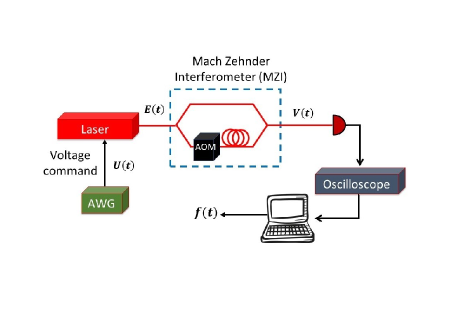
Figure 1: Optical setup for instantaneous laser frequency measurement. An arbitrary waveform generator (AWG) issues the voltage command sent to the laser source. The laser field $E(t)$ enters an unbalanced Mach-Zehnder interferometer containing a frequency shift in its long arm. The beatnote collected on the photodiode is digitized and processed to retrieve the instantaneous laser frequency $f(t)$.

For an incoming laser field $E(t)=E_{0}e^{i(2\pi\nu_{0}t+\phi(t))}$, $\phi(t)$ being the instantaneous phase of the laser, the beatnote signal at the output of the MZI reads as:

$$V(t)\propto 1+\sin{\left(2\pi f_{\mathrm{MZI}}t+\phi(t-\tau_{\textrm{MZI}})-\phi(t)\right)}$$ (1)

The instantaneous frequency $f(t)$, defined as $f(t)=\frac{1}{2\pi}\frac{d\Phi(t)}{dt}$, may then be retrieved from $V(t)$ using the Hilbert transformation [22].

2.2 Distorted laser response and corresponding correction

When the laser frequency is modulated via a modulation input on its current supply, a voltage command $U_{0}(t)$ leads to a distorted frequency excursion $f(t)$. Assuming the laser and current supply operate linearly, this frequency excursion is given by the convolution product of the voltage command and the impulse response $R(t)$ of the system:

$$f(t)=U_{0}(t)\otimes R(t)$$ (2)

To make the laser operate according to the user’s requirement, one can fully characterize the laser and driver’s impulse response $R(t)$ (or, equivalently, its transfer function $H(f)$ expressed in Hz$/$V), and consequently operate the laser with a pre-distorted voltage command $U_{pd}(t)$ given by:

$$U_{pd}(t)={\mathscr{F}}^{-1}\left[\frac{\mathscr{F}[f_{C}(t)](f)}{H(f)}\right]$$ (3)

where $f_{C}(t)$ is the desired frequency excursion and ${\mathscr{F}}$ is the Fourier transform operator.

In the linear regime, such a pre-distortion should efficiently compensate for reproducible laser frequency deviations originating from the non-instantaneous response of the laser and driver. However, residual errors may remain due to actual non-linearity of the laser frequency dependence on the injection current [23]. To address this, an efficient method consists in iteratively modifying the voltage command with a small correction inferred from the previously measured frequency error [17, 18]. More specifically, the $i$-th voltage command is obtained as:

$$U_{i}(t)={\mathscr{F}}^{-1}\left[\frac{[\mathscr{F}[U_{i-1}(t)](f)H(f)+\alpha\mathscr{F}[\epsilon_{i-1}(t)](f)}{H(f)}\right],$$ (4)

$U_{i-1}(t)$ being the previous voltage command, $\epsilon_{i-1}(t)$ the previous frequency error with respect to the desired frequency excursion, and $\alpha$ a numerical parameter chosen between $0$ and $1$ to ensure the convergence.

2.3 Experimental realisation

We implement the aforementioned double correction scheme on a Photodigm DBR laser driven with a fast modulation input current source (Vescent D2-105). The successive voltage commands are generated with an arbitrary waveform generator Tektronix AWG5004. The fully fibered, unbalanced MZI comprises an optical delay $\tau_{\textrm{MZI}}=60$ ns and a $80$ MHz AOM in the same arm. The beatnote signal is collected on a $150$ MHz bandwidth photodiode, sampled with a digital oscilloscope and transferred to a computer to derive the instantaneous frequency of the laser $f(t)$ [22].

Two types of excursion are tested: first, a periodic, triangular frequency excursion comprised of two opposite chirps, with a $800$ MHz chirp span and $100$ kHz modulation frequency. Second, an arbitrary excursion with two opposite $2.5~{}\mu$s-long chirps over a $\pm 750$ MHz range, corresponding to a $300~{}$MHz/$\mu$s chirp rate, separated by a $20~{}\mu$s monochromatic operation interval (see Figure 2). The drive voltage and the corresponding laser response show a strong distortion, with frequency errors as high as $300$ MHz. In the triangular case, we measure a $72.9$ MHz RMS error, equivalent to a $9.1\%$ nonlinearity for the triangular chirps.

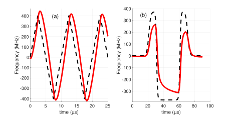
Figure 2: Evidence of the non-instantaneous laser response (solid red line) to a rapidly varying drive voltage (black dashed line), in the case of (a) triangular and (b) arbitrary command.

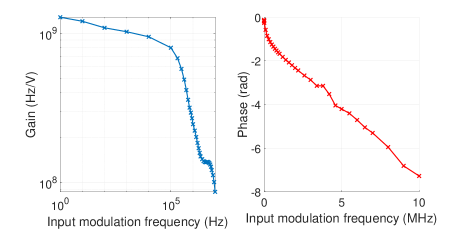
Figure 3: Laser transfer function amplitude and phase when disturbed through the "Current Servo Input" modulation input of the Vescent D2-105 driver. The laser instantaneous frequency is measured with the unbalanced, frequency-shifting MZI. Therefore this transfer function includes the response of this modulation input, that of the laser itself, and the response of the MZI.

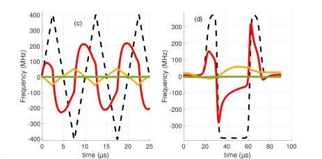
Figure 4: Pre-distorted voltage commands (solid yellow line) and iteratively-corrected voltage commands (solid green line) in order to achieve the desired frequency excursions (black dashed line), in the case of (a) triangular and (b) arbitrary excursion. (c) and (d): frequency errors with a free-running laser (solid red line), with the pre-distorsion (yellow line) and after 20 iterations (solid green line).

In order to implement the pre-distorsion stage, we determine the laser transfer function $H(f)$ in amplitude and phase by sending sinusoidal voltages into the modulation input of the laser current controller and measuring the resulting instantaneous frequency variation of the laser (see Fig. 3). The voltage commands corresponding to triangular and arbitrary frequency excursions are then pre-distorted using Eq. 3. The pre-distortion, operating as an anticipation of the non-instantaneous laser response, leads to a significant improvement of the laser behaviour (see Figure 4): the frequency errors are clearly reduced (of the order of $60$ MHz). For the triangular chirps, the RMS error is reduced to $20.52$ MHz, equivalent to a $2.5\%$ nonlinearity.

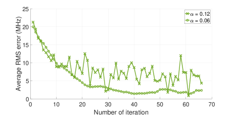
Figure 5: Evolution of the RMS frequency error using the iteration algorithm described in Equation 4, in the case of a triangular $800$ MHz amplitude frequency excursion with $100$ kHz modulation frequency, for two values of the parameter $\alpha$.

In order to further reduce the frequency error, we implement the iterative correction algorithm on both frequency excursions using Equation 4 (see Figure 4). We observe that after few tens of iterations, the frequency error is substantially reduced, down to a few MHz. An $2.1$ MHz RMS error is obtained for the triagular chirps, corresponding to a $0.26\%$ non-linearity. Examining the convergence of the iterative algorithm, we show that larger $\alpha$ values allow a faster convergence but a lower frequency excursion precision (see Figure 5).

3 Suppression of non-reproducible errors

Once the systematic errors are efficiently suppressed, one is left with only stochastic frequency errors, mostly coming from the intrinsic laser frequency noise, but also potentially caused by the steep frequency chirps and abrupt slope changes. We propose a versatile correction able to handle arbitrary frequency commands including fast laser chirps and monochromatic laser operation.

3.1 Phase-Locked-Loop feedback correction

Self-heterodyne systems (such as the unbalanced MZI presented in Section 2.1) enable the generation of an signal proportional to the frequency offset via the downconversion of the detected beatnote with a local oscillator (LO). This signal can then be used as a correction signal to the laser source, resulting in a feedback loop. This setup is analog to an electronic phase-locked-loop (PLL) where the voltage-controlled oscillator (VCO) is composed of the laser source and the interferometer, and the frequency mixer and subsequent filter act as a phase comparator.

We use a versatile version of this setup that consists in using a specific local oscillator $V_{th}(t)$, proportional to the ideal beatnote signal that is expected for an ideal, error-free and noise-free laser frequency excursion, given any arbitrary laser frequency excursion [16].

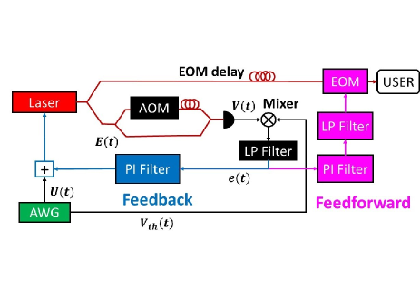
Figure 6: Experimental setup including the feedback loop and the feed-forward correction for arbitrary frequency excursions. The laser current is driven via an arbitrary voltage command generated by an arbitrary waveform generator (AWG) fed into a fast modulation input port. For both corrections, an error signal is produced via the downconversion of the beatnote at the output of the self-heterodyne Mach-Zehnder interferometer. For the feedback loop, this error signal is filtered through a proportional-integrator filter (PI filter) and added to the voltage command to the laser current driver. For the feed-forward correction, the same error signal is filtered with a PI and a low pass filter, and fed into a phase modulator after a physical fibered delay line on the user laser beam.

We experimentally implement this PLL feedback loop using the optical beatnote collected at the output of the MZI (see Section 2.1) and mixing it with the ideal beatnote signal generated by our multichannel AWG5004, using an electronic mixer (Mini-Circuits ZFM.1+). The use of a single device for driving the AOM and creating the LO signal ensures minimal electronic jitter. The resulting signal is filtered with a $10$-MHz, $5$th order Tchebychev low-pass filter. A proportional-integrator loop filter is then used, built with a Newport LB1005S servo-controller operated in Low Frequency Gain Limitation (LFGL) mode with a $1$-MHz PI corner.

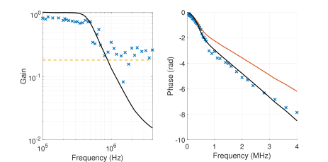
Figure 7: Experimental (dots) and simulated (lines) closed feedback loop transfer function in amplitude (a) and phase (b). The simulated transfer function is derived from the independent measurement of each component of the loop (see Appendix A.1), completed with an additional delay (black lines). The red line shows the transfer function phase without this additional delay. The yellow dashed line shows the detection noise limit.

The transfer function of the closed feedback loop is measured and plotted in Figure 7. A description of the measurement method is given in Appendix A. We observe a sharp cutoff around $600$ kHz. The PLL transfer function exhibits a quasi-linear phase, whose slope corresponds to an effective group delay $\tau_{\textrm{PLL}}=270$ ns where $\Phi(f)=2\pi f\tau_{\textrm{PLL}}$. We demonstrate in Appendix A that this delay corresponds to the physical delay of the various optical and electronic elements in the loop, and that it directly affects the feedback bandwidth via $BW=\frac{1}{8\tau_{PLL}}\simeq 460$ kHz.

3.2 Feed-forward correction

The high frequency fluctuations triggered by fast frequency excursions require an instantaneous frequency correction with a broad bandwidth. To overcome the feedback bandwidth limitation, we propose to combine it with a feed-forward (FF) correction. Feed-forward consists in applying a correction to the laser emission a posteriori, using the knowledge of the current laser behaviour. To achieve this, a phase-modulating device must be used, such as an electro-optic modulator (EOM) or acousto-optic modulator (AOM). An EOM offers a weaker tunability than an AOM but a higher bandwidth, which is key for the correction of high frequency errors. The FF approach has already been proposed for laser frequency stabilization either on its own [24] or combined with feedback [25, 26], but never for laser frequency chirp correction, to our knowledge.

In our design, we propose to generate a FF correction based on the same error signal as the feedback loop after the downconversion step. This error signal is sent to the phase modulator inserted in the user beam (see Fig. 6), after appropriate electronic filtering. Importantly, the quality of the FF correction relies on the application of the correction at the right time. Therefore, to account for the delay naturally occurring in the buildup of the correction signal, a physical delay is inserted before the phase modulator along the user beam.

We implement the FF scheme using a fibered EOM (iXblue MPXLN-0.3) with $300$ MHz bandwidth. The FF correction signal is obtained using the same error signal as the PLL but with a different PI filter, also generated by a Newport LB1005S servo-controller operated in LFGL mode ($1$MHz PI-corner) combined with a low-pass RC filter with $10$ MHz cutoff frequency. The combination of all the optical and electronic elements of the feed-forward correction yields a high-pass behaviour and a total group delay of around $180$ ns (see Appendix B). In order for the FF correction to reach the laser emission at the right time, a $28$ m fibered delay line of (corresponding to a $140$ ns delay) is inserted before the EOM.

We investigate the influence of this physical delay on the quality of the noise compensation and show that the delay has a critical effect on the quality of the feed-forward correction and in turn on the laser linewidth (see Appendix B). Interestingly, in contrast with the feedback correction, the feed-forward bandwidth is only limited by the bandwidth of the various elements of the FF correction signal and remains independent from the feed-forward delay.

3.3 Implementation on a monochromatic laser

Our dynamic, real-time corrections are tested on the DBR laser in monochromatic operation. In Figure 8 we plot the power spectral density (PSD) of the beatnote signal with and without feedback correction. We also plot the local oscillator spectrum to show the lower limit attainable by the feedback. We obtain a noise rejection of about $10$ dB in a $150$ kHz range around the $80$ MHz carrier. One can derive the feedback bandwidth as the frequency at which the beatnote signal PSD reaches the value of the free-running laser beatnote PSD. Such an estimation yields a feedback bandwidth around $440$ kHz, in agreement with the bandwidth derived from the closed loop transfer function (see Section 2.3).

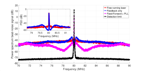
Figure 8: Self-heterodyne beatnote spectra with a monochromatic laser (resolution bandwidth: $10$ kHz). The beatnote spectrum is centered on the driving frequency of the AOM inside the MZI (see Fig. 1). Inset: close-up view with narrower resolution bandwidth ($1$ kHz), allowing a better view of the effect of the feedback loop.

Assessing the influence of the FF correction on the laser spectral purity is less straightforward. Indeed, a second optical frequency discriminator (OFD) is needed [26]. However, using a separate, independent device would lead to relative instability due to uncorrelated acoustic and thermal perturbations. To avoid this we use the same physical OFD as the one used for the error signal generation (see Fig. 9): we simultaneously send the feed-forward-corrected laser beam in the unused port of the MZI, in the backwards direction. The effect of the full correction can then be analyzed by examining the spectrum of the beatnote signal collected on the second photodiode. We obtain a noise rejection in a range of $8$ MHz around the $80$ MHz carrier (see Figure 8). The maximum noise rejection occurs at $2.4$ MHz around the $80$ MHz carrier with 17-dB noise rejection, indicating a FF correction bandwidth around $5$ MHz.

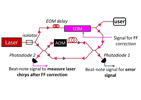
Figure 9: Simultaneous error signal generation and instantaneous laser frequency measurement with a single MZI: the MZI is assembled with $2\times 2$ 3dB fiber couplers allowing two opposite, independent propagation schemes in the same equipment and ensuring perfect relative stability.

We can also analyze the performance of our feedback and feed-forward corrections by examining the laser linewidth and laser spectrum that we derive from the output of a commercial optical frequency discriminator (Silentsys OFD) [27] (see Figure 10). We observe the typical linewidth tendency to increase with the integration time [28], in all configurations. The feedback has a crucial impact on the linewidth on the investigated timescales (above $10~{}\mu$s). The feed-forward correction, on the other hand, is most efficient on shorter timescales where the linewidth cannot be accurately measured. The $740$-kHz linewidth of the free-running laser is reduced down to $81$ kHz with the feedback correction, and further down to $30$ kHz with both the feedback and the feed-forward corrections, for a $100$ ms integration time.

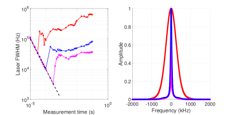
Figure 10: Reconstruction of the laser spectrum in monochromatic operation using the calibrated output signal of a commercial optical frequency discriminator. (a) Laser linewidth (estimated as the FWHM of the reconstructed laser lineshape) for various integration times between $10~{}\mu$s and $100$ ms. The dashed black line represents the Fourier uncertainty that limits the linewidth derivation [28]. (b) Reconstructed laser lineshape for free-running laser (red), feedback-locked laser (blue) and feedback + feed-forward locked laser (magenta), where the frequency noise is integrated over $100$ ms.

4 Implementation of the four-stage correction on complex laser chirps

In this section we test our complete, multistage correction (including pre-distorsion, iterative correction, feedback and feed-forward) on complex frequency excursions on our DBR laser. Two configurations are studied, namely triangular excursions, and the arbitrary excursion with $750$ MHz by $2.5~{}\mu$s chirps described in Section 2.3.

It is important to realize that the feedback and feed-forward correction can only correct relatively small frequency errors. The initial pre-distorsion and iterative corrections, limiting the error to within a few MHz, are an absolute pre-requisite to ensure the proper action of the real-time correction stages. In their absence, the laser frequency error may largely exceed the MZI free spectral range, making the error signal unreliable.

4.1 Triangular excursions

The feedback and feed-forward corrections are implemented on the triangular frequency excursions, using the pre-distorted and iteratively corrected voltage command shown in Figure 4. The laser instantaneous frequency is measured and compared to the desired frequency excursion (see Figure 11). The corresponding RMS frequency error values are computed on several periods and given in Table 1. The feedback correction visibly improves the chirp precision. Nevertheless, the feedback bandwidth limits the correction efficiency as we reach for higher modulation frequencies.

The feed-forward correction further improves the frequency excursion by correcting fluctuations at a faster rate. Nevertheless the sharp angles of the triangular command lead to residual high frequency fluctuations, even with the feed-forward part (see Table 1). We attribute this limitation to the detection noise that is imparted onto the laser emission via the feedback and feed-forward (see Appendix A). An interesting figure of merit to estimate the quality of the correction is the non-linearity of the frequency excursion, ie the ratio between the fluctuation standard deviation $\sigma_{\mathrm{PLL+FF}}$ and the chirp span $\Delta f$. This figure remains well below $1\%$ for all the configurations shown. Note that due to its low-frequency cutoff, the feed-forward correction cannot operate without the feedback correction, due to significant slow frequency noise.

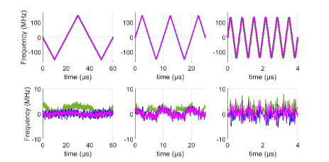
Figure 11: Laser frequency response and respective frequency errors for triangular excursion with pre-distorsion and iterative correction (green lines), iterative correction combined with feedback correction (blue), and with iterative correction and feedback combined with FF correction (magenta). Measurements are performed at different modulation frequencies: $25$, $100$ and $1500$ kHz.

$f_{modulation}$	$\sigma_{iteration}$	$\sigma_{\textrm{PLL}}$	$\sigma_{\mathrm{PLL+FF}}$	non-linearity
$25$ kHz	$2.17$ MHz	$0.79$ MHz	$0.68$ MHz	$0.23\%$
$100$ kHz	$1.99$ MHz	$1.24$ MHz	$1.19$ MHz	$0.40\%$
$1500$ kHz	$2.77$ MHz	$2.19$ MHz	$2.06$ MHz	$0.69\%$

Table 1: Frequency fluctuation performances for triangular excursions with $300$ MHz span. Note that the value of the RMS is computed over several periods of the triangular wave, including the abrupt slope changes.

We test our full multi-stage correction on triangular shapes with increasing chirp span $\Delta f$, keeping the modulation frequency at $25$kHz and $100$kHz. The results are presented in Table 2. Consistently with our earlier findings, we find that each correction stage successfully improves the frequency excursion accuracy. Interestingly, we show that this non-linearity factor improves with increasing chirp span, reaching approximately $0.1\%$ with GHz chirp spans.

$f_{mod}$	$\Delta f$	$\sigma_{\textrm{iteration}}$	$\sigma_{\textrm{PLL}}$	$\sigma_{PLL+FF}$	non-lin
$100$kHz	$300$MHz	$1.99$MHz	$1.24$MHz	$1.19$ MHz	$0.40\%$
	$550$MHz	$1.94$MHz	$1.43$MHz	$1.14$MHz	$0.21\%$
	$800$MHz	$2.26$MHz	$1.55$MHz	$1.46$MHz	$0.18\%$
$25$kHz	$300$MHz	$2.17$MHz	$0.79$MHz	$0.68$MHz	$0.23\%$
	$750$ MHz	$2.48$MHz	$1.19$MHz	$1.04$MHz	$0.14\%$
	$1200$ MHz	$2.26$MHz	$1.55$MHz	$1.46$MHz	$0.12\%$

Table 2: Frequency fluctuation RMS and non-linearity for triangular excursions with various modulation frequencies and chirps spans.

4.2 Arbitrary excursions

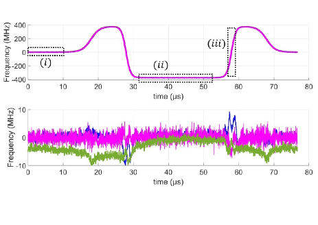
Figure 12: Laser response and respective frequency errors for an arbitrary frequency excursion. The green, blue and magenta lines correspond to iterative correction, iterative correction combined with feedback correction, and iterative correction combined with feedback correction and FF correction, respectively. The frequency error RMS is retrieved in the three rectangular frames: $\sigma_{\mathrm{FF}}=1.45$ MHz, $1.62$ MHz and $1.42$ MHz for $(i)$, $(ii)$ and $(iii)$, respectively.

We now study the effect of our multi-stage correction on the arbitrary frequency excursion, using the pre-distorted and iteratively corrected voltage command described in Section 2 (see Fig. 12).

Similarly to the triangular excursions, the feedback loop only corrects the low frequency fluctuations and adds high-frequency noise. The feed-forward correction efficiently complements the feedback loop as it strongly reduces the remaining frequency excursion imprecisions that occurred at the steep frequency variation points. Remarkably, the RMS frequency error evaluated on the intermediate monochromatic stage $(ii)$ is only marginally deteriorated with respect to the initial RMS error before the $800$ MHz-range perturbation $(i)$. We compute the laser lineshape in the $22~{}\mu$s interval between the two chirps $(ii)$ and obtain a $48$ kHz linewidth, close to the Fourier-transform limit, demonstrating the excellent laser spectral purity although in the midst of an abrupt frequency excursion. Finally, the RMS error in the linear part of the positive slope ($500$ MHz/$2~{}\mu$s) at the end of the arbitrary sequence $(iii)$ is as low as that in monochromatic operation $(i)$. This highlights our multi-stage correction’s versatility, ie its ability to operate on a succession of abrupt frequency chirps and monochromatic operation.

5 Conclusion

A current-modulated laser can be used to generate fast arbitrary frequency excursions with high modulation frequency and large chirp span. However, the inaccuracy of the frequency excursion and the high-frequency fluctuations induced by the fast spectral components of the modulation calls for an efficient and broadband correction design. In this work, a multi-stage correction is developed, including pre-distorsion and iterative correction to suppress systematic errors, and the combination of a feedback loop and a feed-forward correction both based on a self-heterodyne, unbalanced interferometer to suppress both slow and fast stochastic errors up to $5$ MHz.

We test our multi-stage correction on various laser frequency excursions to demonstrate its efficiency and versatility. In monochromatic operation we demonstrate an impressive reduction of the laser linewidth with the combined feedback and feed-forward stages. We also achieve $300$-MHz triangular excursions with a non-linearity below $1\%$ with modulation frequencies up to $1500$ kHz. Finally, we implement this multi-stage correction on an arbitrary frequency excursion with alternating steep slopes and monochromatic segments, and consistently demonstrate $<100$kHz laser spectral purity even in the midst of GHz-scale excursions.

This work opens new possibilities in various application domains including FMCW lidar, telecommunications or wideband signal processing, where fast and accurate laser frequency excursions are required.

Appendix A Appendix: Parameters of the feedback loop

In this section we discuss the relation between the feedback loop parameters and its bandwidth. First, PLL general considerations are presented and applied to our MZI-based feedback loop. Then the influence of the PLL delay on the feedback bandwidth and error correction is studied. Finally, the MZI delay impact on the laser instantaneous frequency measurement and the buildup of the error signal is discussed.

A.1 PLL transfer function

A PLL generally contains the following elements: a local oscillator, a phase comparator, a loop filter, and a voltage-controlled ocillator (VCO) [29]. The Open Loop Transfer Function (OLTF) is the product of the transfer functions of the successive elements of the loop:

$$F_{\mathrm{OL}}(f)=\frac{1}{2i\pi f}K_{\Phi}F_{\mathrm{lf}}(f)K_{\mathrm{VCO}}(f),$$ (5)

where $K_{\Phi}$ is the phase comparator gain such that, when two signals with a $\Delta\Phi$ phase difference are sent to the phase comparator, the following signal is output: $V=K_{\Phi}\Delta\Phi$. $F_{\mathrm{lf}}(f)$ is the loop filter transfer function, and $K_{\mathrm{VCO}}(f)$ is the VCO transfer function. Finally, the Closed Loop Transfer Function (CLTF) is given by:

$$F_{\mathrm{CL}}(f)=\frac{F_{\mathrm{OL}}(f)}{1+F_{\mathrm{OL}}(f)}$$ (6)

In the case of feedback correction on a current-controlled laser (see Section 3 and Figure 6), the VCO includes the laser driver, the laser source and the MZI. Its transfer function, given by $H(f)$, is described and measured in section 2.3 (see Fig. 3). The loop filter is comprised of the servo-controller in PI mode, and a passive, 5-th order low-pass filter with a $10$ MHz cutoff frequency, whose transfer functions are measured separately. The phase comparator, whose role is ensured by the mixer, is also characterized and found to give rise to a significant group delay together with a constant dephasing, so we write $F_{\Phi}(f)=K_{\Phi}e^{-2i\pi f\tau_{\textrm{mix}}-i\Phi_{\mathrm{mix}}}$, with $\tau_{\textrm{mix}}=50$ ns and $\Phi_{\mathrm{mix}}=\pi/4$. Finally the various delays induced by each element of the feedback loop are summarized in Table 3. Finally the OLTF reads as:

$$F_{\mathrm{OL}}(f)=\frac{1}{2i\pi f}F_{\Phi}(f)F_{PI}(f)F_{\mathrm{lp}}(f)H(f)$$ (7)

Component	Transfer function	Group delay
Laser+MZI	$H(f)$	$100$ ns
LB1005	$F_{\mathrm{PI}}(f)$	$40$ ns
Mixer	$F_{\Phi}(f)$	$50$ ns
Low-pass filter	$F_{\mathrm{lp}}(f)$	$44$ ns

Table 3: Effective group delays induced by each element of the feedback loop.

We measure the feedback loop transfer function $F_{\mathrm{CL}}(f)$ by making the laser frequency oscillate with the feedback loop closed. A small amplitude ($8$ MHz), monochromatic frequency modulation is applied on the local oscillator. The closed PLL ensures that the phase of the MZI output matches the phase of the local oscillator, which induces a frequency modulation of the laser source. The resulting instantaneous frequency variations of the laser emission are measured by analyzing the beatnote at the output of the MZI, giving access to the PLL transfer function plotted in Fig. 7. The dynamic range of the gain measurement is limited because the feedback loop parameters must be kept constant for all frequencies, rendering impossible to compensate for the strong attenuation of frequencies above $500$ kHz. In order to accurately account for the experimental transfer function measurements, the simulated transfer function given by Eqs. 6 and 7 is corrected by a small additional delay ($\tau_{\mathrm{extra}}=101$ ns), ascribed to the various electronic and optical delays present in the loop and not explicitly considered in our analysis (free space propagation, coaxial cables, splitters, etc). The simulation finally provides a good understanding of the PLL transfer function, and allows us to estimate the total group delay associated to the feedback loop $\tau_{\textrm{PLL}}=335$ ns, accounting for all its components.

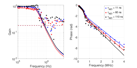
Figure 13: PLL transfer function for 3 different MZI delays: $11$ ns, $60$ ns and $110$ ns. PLL transfer function measurements are plotted for 3 different MZI delays: $11$ ns (blue points), $60$ ns (red points) and $110$ ns (black points). The corresponding theoretical transfer functions for each MZI delay are computed using equations 5 and 6 with the transfer functions of the PLL elements and the corresponding MZI delay: $11$ ns (blue line), $60$ ns (red line) and $110$ ns (black line)

We now explore the impact of the MZI delay on the PLL transfer function. To that end we operate the laser with the feedback correction using various fiber lengths in the MZI (such that $\tau_{\textrm{MZI}}=11$ ns, $60$ ns and $110$ ns). The results plotted in Figure 13 show only a weak dependence of the PLL transfer function, confirming that the MZI delay only contributes marginally to the feedback bandwidth.

A.2 PLL delay and feedback bandwidth

In this section we examine how the group delay-like behavior of the PLL transfer function leads to a bandwidth limitation. Let us assume that the laser exhibits a sinusoidal frequency fluctuation $\epsilon_{0}(t)$ at frequency $F$ with an amplitude $\Delta F$: $\epsilon_{0}(t)=\Delta F\sin(2\pi Ft)$. If the feedback loop is equivalent to a mere delay line, the feedback signal reads as $U_{fb}(t)=G\epsilon_{0}(t-\tau_{\textrm{PLL}})$, where $G$ is the feedback loop gain. After applying the feedback signal to the laser source, the frequency fluctuation becomes $\epsilon(t)=\epsilon_{0}(t)-U_{fb}(t)$. To quantify the effect of this feedback on the laser frequency stability, we examine the variance $\sigma^{2}=\langle\epsilon(t)^{2}\rangle$ of the frequency fluctuations:

$$\sigma^{2}=\Delta F^{2}\left(\frac{G^{2}+1}{2}-G\cos(2\pi F\tau_{\textrm{PLL}})\right)$$ (8)

$\sigma^{2}$ reaches a minimum when $G=\cos(2\pi F\tau_{\textrm{PLL}})$:

$$\sigma_{min}^{2}=\frac{\Delta F^{2}}{2}\sin^{2}(2\pi F\tau_{\textrm{PLL}})$$ (9)

The fluctuation variance with no feedback is $\sigma_{0}^{2}=\frac{\Delta F^{2}}{2}$. The ratio $\frac{\sigma^{2}_{min}}{\sigma_{0}^{2}}$ can be seen as the feedback loop’s ability to correct fluctuations at frequency $F$. To lowest order, this figure of merit quadratically increases with the fluctuation frequency $F$. We define the feedback loop bandwidth as the frequency $F$ for which the aforementioned variance ratio is equal to $\frac{1}{2}$:

$$F_{BW}=\frac{1}{8\tau_{\textrm{PLL}}}$$ (10)

This confirms the common knowledge that a large feedback bandwidth requires a short loop delay $\tau_{\textrm{PLL}}$.

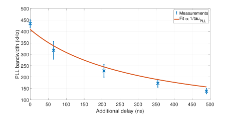
Figure 14: Exploring the effect of adding coaxial delay lines to the feedback loop on the PLL bandwidth. The laser is operated at fixed frequency and the PLL bandwidth is retrieved from the beatnote spectra (analog to Fig. 8). The experimental points are fitted using Eq. 10 and a value $\tau_{\textrm{PLL}}=306\pm 12$ ns is found.

We experimentally examine the influence of the total loop delay on the feedback loop performance. The laser is operated at fixed frequency and the feedback bandwidth is retrieved from the beatnote spectra (analog to Fig. 8). Several values of the PLL delay are explored by adding coaxial delay lines to the existing setup, leading to a total PLL length $\tau_{\textrm{PLL}}+\tau_{\mathrm{coax}}$. The measured bandwidths are shown in Figure 14 and show a $1/(\tau_{\textrm{PLL}}+\tau_{\mathrm{coax}})$ scaling law, in agreement with Eq. 10. By fitting the measurements with the model, we derive $\tau_{\textrm{PLL}}=306\pm 12$ ns.

A.3 MZI delay influence on instantaneous frequency measurement

Although the MZI delay only marginally affects the PLL transfer function and bandwidth, it actually influences the laser frequency measurement precision, because it is involved in the derivation of the error signal. In the following we show that the ideal MZI delay results from a compromise between precision and sensitivity to detection noise.

Instantaneous frequency accuracy

We first analyze how the MZI delay comes into play in the laser instantaneous frequency derivation. This derivation starts with the analytical representation of the beatnote signal at the output of the MZI, whose complex phase is $2\pi f_{\mathrm{MZI}}t+\phi(t-\tau_{\textrm{MZI}})-\phi(t)$. After removing the linear term due to the frequency shift $2\pi f_{\mathrm{MZI}}t$, one is left with the laser phase variation $\phi(t-\tau_{\textrm{MZI}})-\phi(t)$, from which the laser instantaneous frequency is derived:

$$f(t)=-\frac{1}{2\pi}\frac{d\Phi}{dt}\simeq-\frac{1}{2\pi}\frac{\Phi(t)-\Phi(t-\tau_{\textrm{MZI}})}{\tau_{\textrm{MZI}}}$$ (11)

This estimation of the instantaneous frequency is not perfectly accurate. For example, in the case of a linear frequency chirp $\phi(t)=\pi rt^{2}$, Eq. 11 leads to a $\frac{1}{2}r\tau_{\textrm{MZI}}$ inaccuracy of the instantaneous frequency estimation. This inaccuracy increases with the MZI delay [22].

Sensitivity to detection noise

On the other hand, shorter delays increase the sensitivity to detection noise. When the laser is perfectly stable with no frequency drift ($f(t)=0$), the beatnote signal captured by the photodiode is a sinusoid oscillating at the AOM frequency: $V(t)=V_{0}(1+\sin(2\pi f_{\mathrm{MZI}}t)~{})$. In the presence of a monochromatic detection noise at frequency $F$, the voltage becomes $V(t)=V_{0}\left(1+\sin(2\pi f_{\mathrm{MZI}}t)\right)+A\sin(2\pi Ft)$. Once the constant term $V_{0}$ is removed, its instantaneous phase $\psi(t)$ is obtained as the complex argument of the analytic representation of $V(t)$ [22]. Assuming $A\ll V_{0}$, one obtains:

$$\psi(t)=2\pi f_{\mathrm{MZI}}t+\frac{A}{V_{0}}\sin\left(2\pi(F-f_{\mathrm{MZI}})t\right)$$ (12)

After removing the linear phase coming from the fixed frequency shift in the MZI ($2\pi f_{\mathrm{MZI}}t$), the remaining term is multiplied by $\frac{1}{2\pi\tau_{\textrm{MZI}}}$ to derive the instantaneous frequency (according to Equation 11):

$$f(t)=\frac{\frac{A}{V_{0}}}{2\pi\tau_{\textrm{MZI}}}\sin\left(2\pi(F-f_{\mathrm{MZI}})t\right)$$ (13)

Therefore the instantaneous frequency derivation converts the detection noise into instantaneous frequency measurement noise. The variance of such frequency fluctuations is given by:

$$\sigma_{\mathrm{det}}^{2}(F)=\frac{(\frac{A}{V_{0}})^{2}}{8\pi^{2}\tau_{\textrm{MZI}}^{2}}$$ (14)

This frequency-independent, $1/\tau_{\textrm{MZI}}^{2}$ scaling law shows that a long MZI delay minimizes the influence of electronic noise.

Generalizing to a white detection noise, the power spectral density of the apparent laser frequency noise should also scale as $1/\tau_{\textrm{MZI}}^{2}$. We verify this by measuring the free-running laser frequency variance using different MZI delay lengths (see Fig. 15). We observe that the frequency noise variance is compatible with the sum of two terms:

$$\sigma^{2}=\sigma_{\mathrm{laser}}^{2}+\sigma_{\mathrm{det}}^{2}$$ (15)

where $\sigma_{\mathrm{laser}}^{2}$ is the native laser frequency noise variance and $\sigma_{\mathrm{det}}^{2}\propto 1/\tau_{\textrm{MZI}}^{2}$ corresponds to the contribution of detection noise.

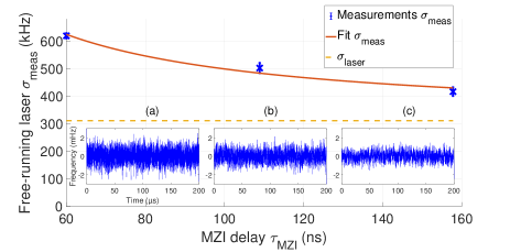
Figure 15: Influence of the MZI delay on the occurence of detection noise. The RMS frequency error is measured over a $200~{}\mu$s interval for different MZI delays. The laser is operated in free-running mode (no feedback or feed-forward) at fixed frequency. The measurements are fitted using Eq. 15 with $\sigma_{\mathrm{laser}}=310$ kHz. Insets: corresponding instantaneous frequency measurements: (a) $60$ ns (b) $108.9$ ns and (c) $158$ ns.

Conclusion

As a result, although the MZI delay has little influence on the PLL bandwidth, it has a strong impact on the accuracy of the instantaneous derivation on the one hand, and on the transduction of electronic noise onto the instantaneous frequency measurement. We finally choose a delay of $60$ ns, as a compromise between precision and sensitivity to detection noise.

Appendix B Appendix: Feed-forward

In this section we discuss the feed-forward theoretical transfer function and the influence of the EOM delay. We show that the optimal delay can be determined by minimizing the laser linewidth.

B.1 Feed-forward delay

The buildup of the feed-forward correction signal is subject to a time delay $\tau_{\mathrm{FF}}$ owing to the various optical and electronic components of the feed-forward setup:

$$\tau_{\mathrm{FF}}=\frac{-1}{2\pi}\frac{\partial\Phi_{\mathrm{FF}}}{\partial f}$$ (16)

where

$$\Phi_{\mathrm{FF}}=\arg\left[F_{\mathrm{MZI}}(f)F_{\Phi}(f)F_{\mathrm{FF}}(f)F_{\mathrm{lp}}(f)F_{\mathrm{EOM}}(f)\right]$$ (17)

$F_{\mathrm{MZI}}$, $F_{\Phi}$, $F_{\mathrm{FF}}$, $F_{\mathrm{lp}}$, $F_{\mathrm{EOM}}$ are the transfer functions of the MZI, the phase comparator, the feed-forward PI filter, the low-pass filter, and the electro-optic modulator, respectively. Some of these transfer functions can be measured independently, namely $F_{\Phi}$, $F_{\mathrm{FF}}$, and $F_{lp}$. Measuring the transfer function of an EOM requires a means to measure an instantaneous frequency in the optical domain. This is why it is most convenient to measure the combined transfer functions of the EOM and the MZI: $F_{\mathrm{MZI}}(f)F_{\mathrm{EOM}}(f)$. We are finally able to compute the product of all these transfer functions, and we plot them in Fig. 16. We find that the feed-forward signal is high-pass filtered due to the derivator behaviour of the EOM. It exhibits a linear phase $\Phi_{\mathrm{FF}}(f)$, indicating an effective group delay $\tau_{\mathrm{FF}}=183$ ns. This delay corresponds to the sum of all individual group delays of each element of the feed-forward correction, which are specified in Table 4.

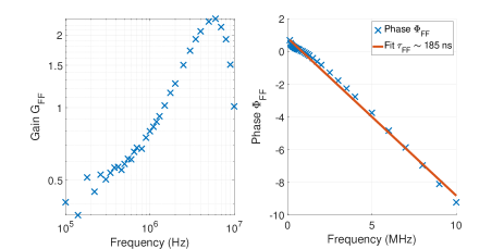
Figure 16: Feed-forward transfer function. The feed-forward exhibits a high-pass behaviour due to the derivator behavior of the EOM. Nevertheless, a cutoff is observed above $5$ MHz due to the MZI response, determining the FF bandwidth. The ideal length of the fibered delay line $\tau_{\mathrm{EOM}}$ is derived from the slope of the transfer function phase (see Eq. 17).

Component	Transfer function	Group delay
EOM	$F_{\mathrm{MZI}}(f)F_{\mathrm{EOM}}(f)$	$90$ ns
Mixer	$F_{\Phi}(f)$	$50$ ns
LB1005	$F_{\mathrm{PI}}(f)$	$40$ ns
Low-pass filter	$F_{\mathrm{lp}}(f)$	$15$ ns

Table 4: Effective group delays induced by each element of the feed-forward correction.

B.2 Influence of EOM delay mismatch

The feed-forward optimally corrects the laser frequency deviations when the delay $\tau_{\mathrm{FF}}$ experienced by the correction signal to reach the EOM matches the physical delay $\tau_{\mathrm{EOM}}$ experienced by the laser beam to reach that same device. In this section we study the influence of a feed-forward delay mismatch $\delta\tau_{\mathrm{EOM}}$ on the laser linewidth. To that end we unfold a simple theoretical approach.

Let us first assume that the laser source exhibits a sinusoidal frequency fluctuation $\epsilon_{0}(t)=\Delta F\sin(2\pi Ft)$. We consider that the feed-forward correction signal $G\epsilon_{0}(t-\delta\tau_{\mathrm{EOM}})$ is applied to the EOM with a temporal mismatch $\delta\tau_{\mathrm{EOM}}$, leading to a corrected frequency fluctuation:

$$\epsilon(t)=\Delta F\left(\sin\left[2\pi Ft\right]-G\sin\left[2\pi F(t-\delta\tau_{\mathrm{EOM}})\right]\right)$$ (18)

The frequency fluctuation variance $\sigma^{2}(F)$, defined as: $\sigma^{2}=\langle\epsilon(t)^{2}\rangle$ is given by:

$$\sigma^{2}(F)=\Delta F^{2}\left(\frac{G^{2}+1}{2}-G\cos(2\pi F\delta\tau_{\mathrm{EOM}})\right)$$ (19)

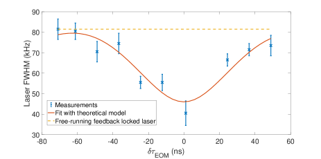
Figure 17: Influence of a feed-forward delay mismatch $\delta\tau_{\mathrm{EOM}}$ on the laser linewidth ($10$ ms integration time). The latter is measured with a stabilized optical frequency discriminator (SilentSys). Zero $\delta\tau_{\mathrm{EOM}}$ corresponds to the optimised FF delay.

We now consider that the laser is affected by a white frequency noise, ie the perturbation is uniform for all frequencies. The laser linewidth is proportional to the total variance of the laser frequency fluctuations [30]:

$$\sigma^{2}_{tot}=\frac{1}{F_{max}-F_{min}}\int_{F_{min}}^{F_{max}}\sigma^{2}(F)dF$$ (20)

where $F_{max}$ and $F_{min}$ are the maximum and minimum frequency addressed by the feed-forward correction. Assuming $F_{min}\ll F_{max}$, one obtains:

$$\sigma^{2}_{tot}=\Delta F^{2}\left(\frac{G^{2}+1}{2}-G\frac{\sin(2\pi\delta\tau_{\mathrm{EOM}}F_{max})}{2\pi\delta\tau_{\mathrm{EOM}}F_{max}}\right)$$ (21)

This expression shows that the laser linewidth is minimal when $\delta\tau_{\mathrm{EOM}}=0$, in agreement with empirical measurements reported in [26]. It also highlights that finding such a minimum is easier when the feed-forward bandwidth is reduced. We verify this behaviour by measuring the DBR laser linewidth with a range of values for the EOM delay around the optimal $\tau_{\mathrm{EOM}}$, using optical fibers with different lengths (see Figure 17). Fitting the experimental data with expression 21, we find the actual feed-forward correction bandwidth $F_{max}=5.7\pm 0.6$ MHz.

Funding The authors acknowledge support from the French National Research Agency (ANR) through the ATRAP project (ANR-19-CE24-0008). This work has received support under the program “Investissements d’Avenir” launched by the French Government.

Acknowledgments The authors are grateful to Michel Lintz and Vincent Crozatier for helpful discussions.

DisclosuresThe authors declare no conflicts of interest.

Data availability Data underlying the results presented in this paper are not publicly available at this time but may be obtained from the authors upon reasonable request.

References

- [1] I. Gazizov, S. Zenevich, and A. Rodin, “Low-pixel-count imaging fmcw lidar,” \JournalTitleAppl. Opt. 61, 9241–9246 (2022).
- [2] X. Zhang, J. Pouls, and M. C. Wu, “Laser frequency sweep linearization by iterative learning pre-distortion for fmcw lidar,” \JournalTitleOpt. Express 27, 9965–9974 (2019).
- [3] L. A. Kranendonk, R. J. Bartula, and S. T. Sanders, “Modeless operation of a wavelength-agile laser by high-speed cavity length changes,” \JournalTitleOptics Express 13, 1498–1507 (2005).
- [4] W. R. Babbitt, Z. W. Barber, S. H. Bekker, et al., “From spectral holeburning memory to spatial-spectral microwave signal processing,” \JournalTitleLaser Physics 24, 094002 (2014).
- [5] A. Kinos, D. Hunger, R. Kolesov, et al., “Roadmap for rare-earth quantum computing,” \JournalTitlearXiv preprint arXiv:2103.15743 (2021).
- [6] L. Levin, “Mode-hop-free electro-optically tuned diode laser,” \JournalTitleOptics letters 27, 237–239 (2002).
- [7] V. Crozatier, G. Gorju, F. Bretenaker, et al., “Phase locking of a frequency agile laser,” \JournalTitleApplied physics letters 89 (2006).
- [8] M. Li, L. Chang, L. Wu, et al., “Integrated Pockels laser,” \JournalTitleNature communications 13, 5344 (2022).
- [9] R. Nagarajan and J. E. Bowers, “High-speed lasers,” \JournalTitleSemiconductor Lasers I pp. 177–290 (1999).
- [10] L. Westbrook, A. Nelson, P. Fiddyment, and J. Collins, “Monolithic 1.5 m hybrid dfb/dbr lasers with 5 nm tuning range,” \JournalTitleElectronics letters 23, 957–959 (1984).
- [11] X. Pan, H. Olesen, and B. Tromborg, “Modulation characteristics of tunable dfb/dbr lasers with one or two passive tuning sections,” \JournalTitleIEEE Journal of Quantum Electronics 25, 1254–1260 (1989).
- [12] W. Zheng and G. Taylor, “Determination of the photon lifetime for dfb lasers,” \JournalTitleIEEE Journal of Quantum Electronics 43, 295–302 (2007).
- [13] W. Yi, Z. Li, Z. Zhou, et al., “Frequency-modulated chirp signals for single-photodiode based coherent lidar system,” \JournalTitleJournal of Lightwave Technology 39, 4661–4670 (2021).
- [14] M. Laroche, C. Bartolacci, G. Lesueur, et al., “Serrodyne optical frequency shifting for heterodyne self-mixing in a distributed-feedback fiber laser,” \JournalTitleOptics letters 33, 2746–2748 (2008).
- [15] I. Y. Poberezhskiy, B. Bortnik, J. Chou, et al., “Serrodyne frequency translation of continuous optical signals using ultrawide-band electrical sawtooth waveforms,” \JournalTitleIEEE journal of quantum electronics 41, 1533–1539 (2005).
- [16] N. Satyan, A. Vasilyev, G. Rakuljic, et al., “Precise control of broadband frequency chirps using optoelectronic feedback,” \JournalTitleOptics express 17, 15991–15999 (2009).
- [17] G. Kervella, J. Maxin, M. Faugeron, et al., “Laser sources for microwave to millimeter-wave applications,” \JournalTitlePhotonics Research 2, B70–B79 (2014).
- [18] G. Lihachev, A. Bancora, V. Snigirev, et al., “Frequency agile photonic integrated external cavity laser,” \JournalTitlearXiv preprint arXiv:2303.00425 (2023).
- [19] P. Li, T. Yang, J. Yang, et al., “The nonlinear tuning technique of a dfb laser using frequency predistortion procedures,” in Terahertz, RF, Millimeter, and Submillimeter-Wave Technology and Applications XIII, vol. 11279 (SPIE, 2020), pp. 250–255.
- [20] X. Cao, K. Wu, C. Li, et al., “Highly efficient iteration algorithm for a linear frequency-sweep distributed feedback laser in frequency-modulated continuous wave lidar applications,” \JournalTitleJOSA B 38, D8–D14 (2021).
- [21] J. Zhang, C. Gao, M. Xue, and R. Liu, “Research on frequency modulation character of the current driven dfb semiconductor laser,” \JournalTitleModern Physics Letters B 33, 1850422 (2019).
- [22] T.-J. Ahn and D. Y. Kim, “Analysis of nonlinear frequency sweep in high-speed tunable laser sources using a self-homodyne measurement and hilbert transformation,” \JournalTitleApplied optics 46, 2394–2400 (2007).
- [23] M. Funabashi, H. Nasu, T. Mukaihara, et al., “Recent advances in dfb lasers for ultradense wdm applications,” \JournalTitleIEEE Journal of selected topics in quantum electronics 10, 312–320 (2004).
- [24] F. Aflatouni and H. Hashemi, “Wideband tunable laser phase noise reduction using single sideband modulation in an electro-optical feed-forward scheme,” \JournalTitleOptics letters 37, 196–198 (2012).
- [25] Y. S. Cheng, B. Szutor, and D. T. Reid, “Feed-forward stabilization of a single-frequency, diode-pumped pr: Ylf-cr: Licaf laser operating at 813.42 nm,” \JournalTitleOptics Express 30, 42902–42911 (2022).
- [26] M. Lintz, D.-H. Phung, J.-P. Coulon, et al., “Note: Efficient diode laser line narrowing using dual, feed-forward+ feed-back laser frequency control,” \JournalTitleReview of Scientific Instruments 88 (2017).
- [27] G. Di Domenico, S. Schilt, and P. Thomann, “Simple approach to the relation between laser frequency noise and laser line shape,” \JournalTitleApplied optics 49, 4801–4807 (2010).
- [28] N. Von Bandel, M. Myara, M. Sellahi, et al., “Time-dependent laser linewidth: beat-note digital acquisition and numerical analysis,” \JournalTitleOptics Express 24, 27961–27978 (2016).
- [29] A. Blanchard, Phase-locked loops: Application to coherent receiver design (1976).
- [30] D. S. Elliott, R. Roy, and S. J. Smith, “Extracavity laser band-shape and bandwidth modification,” \JournalTitlePhys. Rev. A 26, 12–18 (1982).