FFT-based Selection and Optimization of Statistics for Robust Recognition of Severely Corrupted Images

Abstract

Improving model robustness in case of corrupted images is among the key challenges to enable robust vision systems on smart devices, such as robotic agents. Particularly, robust test-time performance is imperative for most of the applications. This paper presents a novel approach to improve robustness of any classification model, especially on severely corrupted images. Our method (FROST) employs high-frequency features to detect input image corruption type, and select layer-wise feature normalization statistics. FROST provides the state-of-the-art results for different models and datasets, outperforming competitors on ImageNet-C by up to $37.1\%$ relative gain, improving baseline of $40.9\%$ mCE on severe corruptions.

Index Terms—  Robustness, Object Recognition, Corruptions, Fourier Transform

1 Introduction

Achieving robustness of object recognition models on corrupted images is a challenging problem, which has been studied extensively in recent years [1, 2, 3, 4, 5]. While the models have achieved impressive results on several benchmarks [6, 7], recent works show that their performance is severely degraded when dealing with corrupted images. Addressing the robustness issues is important to ease the adoption of the models in practical applications on devices used in the wild, where such corruptions are frequently experienced. We tackle this problem considering a collection of image distortions that are commonly observed in real-world natural images. Object recognition using distorted image datasets can be posed as a dataset shift problem [8]. Although there has been substantial prior work investigating this problem, it is far from being fully understood, let alone solved. The most successful approaches make use of data augmentation [9, 10, 11, 12] and adversarial training [13, 5, 2].

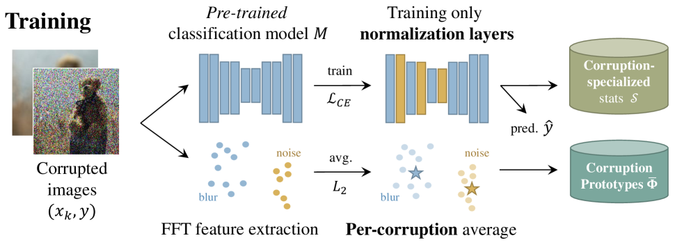
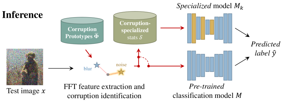
Fig. 1: Overall pipeline of our FROST. At training time, we construct (i) corruption-specific prototypes using high-frequency FFT features and (ii) corruption-specific feature normalization statistics. At test time, we extract FFT features and perform inference via prototype matching to select the most suitable statistics.

Some methods focus on resolving shift of data statistics to improve model robustness, developing modules on top of feature normalization layers [3, 14, 15]. Recent studies leveraged frequency spectra insights to improve model robustness [4, 2, 5]. However, these methods often use cumbersome ensemble models [16] or formulate complex augmentation regimes [17, 5] at training time, with no possibility to adapt the models to test data. In addition, it is important to preserve, if not improve the accuracy of the models on clean samples while enhancing its robustness.

We improve robustness of models against corrupted images by selecting layer-wise feature normalization statistics depending on the corruption via high-frequency features. At test-time, we determine the corruption present in an input image, by processing FFT features and matching them to corruption-specific prototypical features (prototypes). Then, we use codebooks mapping prototypes to corruption-specific statistics provided by normalization layers of models, to adapt the models to input image corruption. Our main contributions can be summarized as follows: (1) we propose a novel test-time FFT-based RObust STatistics selection method (FROST) based on a codebook mapping FFT features to corruption-specific statistics; (2) we achieve model robustness to image corruptions at test-time, making it useful for mobile and robotic applications in the wild; (3) we improve accuracy against competitors on ImageNet-C [1], especially in case of severe corruptions, while preserving accuracy on clean data; (4) our solution is portable to different models and architectures, optimizing statistics of feature normalization layers (Batch/Layer Normalization), with very limited storage requirements.

2 Method

In this section, we introduce the details of our method. FROST (Fig. 1) performs a 2-step approach: At training time, FROST extracts high-frequency amplitudes from corrupted images, it aggregates them for images with the same corruption, and it builds a set of per-corruption feature prototypes. Then, it estimates corruption-specific (Corr-S) and corruption-generic (Corr-G) normalization layer parameters starting from a pretrained model. At test time, FROST identifies corruption types $\hat{k}$ present in the test images and uses a codebook $\mathcal{C}$ to map such corruptions to normalization layers’ parameters to minimize the recognition error. These normalization parameters $\mathcal{S}^{\prime}_{\hat{k}}$ come from either corruption-generic or specific model, depending on the confidence of the model.

Background. Given a model $M$ that approximates ground truth labels $y\in\mathcal{Y}$ of samples $\mathbf{x}\in\mathcal{X}$ using a training set $\mathcal{T}=\mathcal{X}\times\mathcal{Y}$. We define a corrupted image by ${\tilde{\mathbf{x}}=\mathbf{x}+\psi}$, where ${\mathbf{x}\in\mathbb{R}^{w\times h\times 3}}$ is a clean RGB image with the width $w$, height $h$ and corruption $\psi$. Our goal is to improve object recognition accuracy of $M$ on the corrupted images.

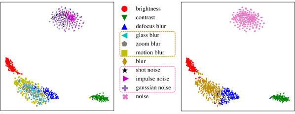
(a)    Original                                        k-means

Fig. 2: t-SNE projection of FFT features. Grouping indistinguishable clusters (i.e., noise and blur except defocus blur), no significant difference is visible between the ground truth and k-means ones. Our method produces FFT features similar to ground truth ones.

Corruptions. Previous works [1, 9] showed that a real corruption $\psi$ can be approximated by a combination of synthetic corruptions. We use a subset $\mathcal{K}=\{$Contrast, Brightness, Defocus Blur, Glass Blur, Motion Blur, Zoom Blur, Impulse Noise, Shot Noise, Gaussian Noise$\}$ of the $9$ most common real corruptions defined in [1]. We denote a synthetic corruption for the clean image $\mathbf{x}$ by $\psi_{k}^{\lambda}(\mathbf{x})$ such that $\mathbf{x}+\psi_{k}^{\lambda}(\mathbf{x})\approx\tilde{\mathbf{x}}$ for $k\in\mathcal{K}$ (e.g., $k=$ Contrast). The parameter $\lambda\in\{1,2,3,4,5\}$ is an integer number which defines corruption intensity depending on the degradation level, with $\lambda=1$ being the lowest and $\lambda=5$ the highest.

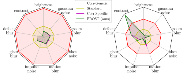
(a)        Mean                                     Variance

Fig. 3: Variation of normalization layers statistics between standard pretrained model (on clean data), corruption-generic $\mathcal{S}_{\mathcal{DA}}$ (Corr-G) model, corruption-specific (Corr-S) model, and normalization statistics of FROST, obtained aggregating them according to similar corruptions.

Model	FFT	BN	Contrast	Defocus B.	Glass B.†	Motion B.†	Zoom B.†	Impulse N.‡	Shot N.‡	Gaussian N.‡	Brightness	mCE	Error
Standard			79	82	90	84	80	82	80	79	65	80.1	23.9
Patch Uniform [18]			77	74	83	81	77	70	68	67	62	73.2	24.5
AA [10]			70	77	83	80	81	72	68	69	56	72.9	22.8
Random AA [10]			75	80	86	82	81	72	71	70	61	75.3	23.6
MaxBlur Pool [19]			68	74	86	78	77	76	74	73	56	73.6	23.0
SIN [20]			69	77	84	76	82	70	70	69	65	73.6	27.2
APR [4]	$\checkmark$		61	72	86	72	79	64	68	62	58	69.1	25.5
BN [14]		$\checkmark$	63	66	62	88	63	72	109	51	36	67.9	—
AugBN [15]		$\checkmark$	60	65	60	86	63	70	106	50	36	66.4	—
AugMix [12]			58	70	80	66	66	67	66	65	58	66.2	22.4
PixMix [11]			53	73	88	77	76	51	52	53	56	64.3	22.6
DA [21]			64	63	75	69	75	45	47	46	55	59.9	23.4
HA [2]	$\checkmark$		68	62	75	69	73	55	58	57	61	64.2	24.4
AugMix+DA+HA	$\checkmark$		54	52	66	54	65	44	46	46	53	53.3	24.9
FROST0.1 (Ours)	$\checkmark$	$\checkmark$	31	35	62	43	54	58	68	60	35	49.4	28.0
FROST0.2 (Ours)	$\checkmark$	$\checkmark$	31	40	57	36	48	44	45	46	41	43.0	26.1
			44.8	54.5	74.7	74.2	77.9	41.0	38.1	44.3	84.4	59.3

Table 1: Analyses of the Corruption Error (CE) $\downarrow$ for the ResNet50 on the ImageNet-C, which is computed by an average of the single errors on the 5 corruptions and compared to the classification error obtained using AlexNet, as in [1]. Error $\downarrow$ is the error of the model on clean images. mCE $\downarrow$ is the classification error averaged on all the aforementioned corruptions. Codebook results are reported in terms of accuracy $\uparrow$.

Model	FFT	BN	Contrast	Defocus B.	Glass B.†	Motion B.†	Zoom B.†	Impulse N.‡	Shot N.‡	Gaussian N.‡	Brightness	mCE	Error
Standard			73	95	110	102	85	94	96	95	58	89.7	23.9
BN [14]		$\checkmark$	100	88	92	110	88	87	150	65	46	91.6	—
AugMix+DA+HA	$\checkmark$		78	68	85	73	79	54	64	58	56	68.4	24.9
AugBN [15]		$\checkmark$	60	65	60	86	63	70	106	50	36	66.4	—
FROST0.2 (Ours)	$\checkmark$	$\checkmark$	30	51	75	51	60	54	59	58	51	54.1	26.1
FROST0.1 (Ours)	$\checkmark$	$\checkmark$	30	44	75	51	61	40	60	45	33	48.8	28.0
			98.0	92.4	90.8	85.5	86.8	83.0	46.2	79.0	80.9	87.5

Table 2: Analyses of the Corruption Error (CE) $\downarrow$ for the ResNet50 on the ImageNet-C on severe corruptions (i.e., severity levels $\lambda=4,5$), which is computed by an average of the single errors on the 2 corruptions and compared to the classification error obtained using AlexNet, as in [1]. Error $\downarrow$ is the error of the model on clean images. mCE $\downarrow$ is the mean corruption error.

Training.    FFT features extraction. For each synthetic corruption in $\mathcal{K}$, we construct a set ${\mathcal{X}}_{k}^{5}$, by applying a corruption $\psi_{k}^{5}(\mathbf{x})$ to all the images $\mathbf{x}\in\mathcal{X}$. In this case, we use only the strongest corruption ($\lambda=5$) to obtain a better separation between features for different corruptions. For each image $\tilde{\mathbf{x}}_{k}=\mathbf{x}+\psi_{k}^{\lambda}(\mathbf{x})$ with corruption $k$, we extract an FFT feature $\Phi_{k}=\mathfrak{F}_{n}(\tilde{\mathbf{x}}_{k})$ by performing FFT $\mathfrak{F}(\cdot)$ [22] on the input image, applying windowing operation to retain the first $n$ high-frequency components of the amplitude spectrum and flattening. In particular, $n$ is selected empirically as $n=15$, computing $\mathfrak{F}(\cdot)$ on images resized to $64\times 64$. Then, we average each set of features specific to corruption $k$ to obtain a prototype $\bar{\Phi}_{k}=\frac{1}{N}\sum_{\tilde{\mathbf{x}}_{k}\in\tilde{\mathcal{X}}_{k}}{\Phi_{k}},\forall k\in\mathcal{K}$, with $N$ being the size of the training set. This can be done via a running average during training with no need to store all features into memory. We call this set $\bar{\Pi}$. Analyzing the set of features $\{\Phi_{k}\}_{k\in\mathcal{K}}$ for different corruptions, we note that some results are very well clustered (e.g., Contrast, Brightness and Defocus Blur), while others (e.g., Blur types and Noise distortions) are hardly separable. To obtain a better clustering score, we compute k-means on the set $\{\Phi_{k}\}_{k\in\mathcal{K}}$ of FFT features (see Fig. 2). This set is originally labeled with corruption-relative labels $L$ from $\mathcal{K}$. Let us define a new labeling $L^{*}$ obtained through k-means. Setting empirically the number of clusters for the k-means to $5$, we obtain similar clustering score as for original labels. In particular, if we group together Blur corruptions, and Noise corruptions, we obtain a new labeling $L^{\prime}$. Comparing $L^{*}$ with $L^{\prime}$ via quantitative analysis, we get an adjusted random score [23] of $89.1\%$ (meaning that the clusters are very similar). For this reason, we aggregate prototypes for features belonging to similar corruptions, obtaining a new set of corruptions ${\mathcal{K}^{\prime}=\{\textit{Contrast},\textit{Brightness},\textit{Defocus},\textit{Blur},\textit{Noise}\}}$ with $5$ macro corruptions. Also, we obtain a new set of macro prototypes $\bar{\Pi}^{\prime}$ averaging prototypes with really close corruptions.

Note that in real-world cases, high-frequency visual content could interfere with the corruption-related frequency content. In those cases, the algorithm can be extended adopting a multi-feature [24] or a multi-scale [25] FFT approach.

Estimation of corruption-specific statistics. We define by $S$ the set of statistics estimated at all normalization layers (Batch/Layer Normalization) in the recognition model $M$. These layers are storage-friendly as they have only two parameters (scale $\gamma$ and shift $\beta$) that have shown to adapt differently to input images affected by different corruptions [3, 9]. Therefore, our purpose is to use it to improve recognition accuracy for corrupted images. First, we train a model $M$ (updating only normalization layers with $S$ parameters) on $\mathcal{T}$ performing data augmentation ($\mathcal{DA}$) on clean samples by adding $\psi_{k}^{\lambda}(\cdot)$. Image augmentations are selected according to a uniform distribution using original corruption functions for augmentations ($K=9$ in total) with severe corruptions only, i.e., $\lambda\sim\{4,5\}$. With this training, we obtain corruption-generic normalization statistics $S_{\mathcal{DA}}$. Then, we train $M$ (updating only normalization layers with $S$ parameters) on $\mathcal{T}_{k}^{4,5}$ (i.e., $\mathcal{T}$ corrupted with corruption $k$, only using $\lambda\sim\{4,5\}$), producing $K$ different corruption-specific sets of normalization statistics $S_{k}$. According to macro corruption grouping $\mathcal{K}^{\prime}$, we average normalization statistics for indistinguishable corruptions obtaining $S^{\prime}_{k}$ sets, one for each macro corruption.

	Contrast		Defocus B.		Glass B.†		Motion B.†		Zoom B.†		Impulse N.‡		Shot N.‡		Gaussian N.‡		Brightness		Average			Clean
	$\lambda_{4}$	$\lambda_{5}$	$\lambda_{4}$	$\lambda_{5}$	$\lambda_{4}$	$\lambda_{5}$	$\lambda_{4}$	$\lambda_{5}$	$\lambda_{4}$	$\lambda_{5}$	$\lambda_{4}$	$\lambda_{5}$	$\lambda_{4}$	$\lambda_{5}$	$\lambda_{4}$	$\lambda_{5}$	$\lambda_{4}$	$\lambda_{5}$	$\lambda_{4}$	$\lambda_{5}$	Tot
Corr-S	69.9	67.4	65.7	63.3	65.9	60.4	68.1	66.9	64.3	62.0	67.3	62.7	66.5	63.6	66.5	61.7	69.0	66.9	67.0	63.9	65.1	73.1
B	13.0	4.1	25.8	17.0	32.3	19.2	23.8	17.6	24.1	18.3	4.8	1.6	4.6	1.8	5.0	1.6	44.3	32.6	19.7	12.6	13.4	73.1
B + $\mathcal{DA}$	60.2	52.6	59.1	54.6	62.1	55.7	62.0	57.4	60.2	56.2	64.2	58.9	63.5	60.0	63.7	57.9	57.0	52.8	61.3	56.2	59.3	72.2
B + $\mathcal{C}$	62.2	59.4	62.4	60.4	53.7	48.4	52.1	41.6	49.1	43.8	54.1	61.6	60.6	62.1	51.0	60.7	65.0	60.3	56.7	55.4	56.0	70.0
	82.7	81.2	92.6	100	89.7	94.4	88.2	92.5	77.9	99.8	84.6	77.1	90.9	98.6	84.2	86.7	72.0	99.4	84.8	92.0	88.4
B + $\mathcal{DA}$ + $\mathcal{C}$	68.7	66.6	65.1	62.7	62.6	55.8	63.6	57.5	60.0	56.1	67.2	62.0	61.5	62.3	66.0	62.0	66.7	63.8	64.6	61.0	62.5	69.1
	92.6	100	89.7	94.4	88.2	92.5	84.6	77.1	84.2	86.7	77.9	98.7	90.9	97.7	72.0	99.4	82.7	81.2	84.8	92.0	89.2

Table 3: Accuracy $\uparrow$ using the ResNet18 with the Tiny-ImageNet. We report the results for a standard model pretrained on clean images (B), Corr-G model (B + $\mathcal{DA}$), Codebook applied only on top of the standard model (B + $\mathcal{C}$) and FROST using the standard model (B + $\mathcal{DA}$ + $\mathcal{C}$). Codebook results are reported below the relative experiment. Blur (†) corruptions and Noise (‡) corruptions share the same model, respectively. Bold indicates the best result and underline indicates the second best result. $\lambda=4$, $\lambda=5$ are shorten with $\lambda_{4},\lambda_{5}$. Tot is the total average on all severe corruptions.

Model	Dataset	Stats	Corr-G	FROST	Clean
ResNet18 [26]	Tiny-ImageNet [7]	BN	59.3	62.5  (89.2)	69.1
ResNet50 [26]	Tiny-ImageNet [7]	BN	66.7	68.6  (88.6)	74.0
ResNet101 [26]	Tiny-ImageNet [7]	BN	74.9	76.5  (84.9)	81.5
ViT-B [27]	Tiny-ImageNet [7]	LN	71.6	73.7  (87.2)	79.0
ViT-L [27]	Tiny-ImageNet [7]	LN	82.5	84.6  (85.9)	85.2
ResNet18 [26]	CIFAR10 [7]	BN	53.5	54.2  (86.8)	70.1
ResNet18 [26]	CIFAR100 [7]	BN	31.6	32.1  (83.6)	46.6

Table 4: Average accuracy $\uparrow$ on the corruption generic (Corr-G) model, FROST on corruptions and Clean data, using different datasets and networks. Codebook results are reported in brackets.

Inference.    At test time, we use prototypical features $\bar{\Pi}^{\prime}$ as keys of a codebook $\mathcal{C}$ to select the best set $S^{*}$.

Prototype matching. We perform inference on each test image $\tilde{\mathbf{x}}_{u}$ with unknown corruption $u$. First, we extract feature $\Phi_{u}=\mathfrak{F}_{n}(\tilde{\mathbf{x}}_{u})$, retaining the first $n$ high-frequency components of the FFT amplitude spectrum. Then, we compute the probability that image is corrupted with corruption $k$ such that $p(u=k)=\text{dist}_{\ell_{2}}(\Phi_{u},\bar{\Phi}_{k})$ for each corruption $k\in\mathcal{K}^{\prime}$ using $\ell_{2}$ distance. Note that a test image can also be non-corrupted; we will explain how this case is handled in the next paragraph.

Selection of statistics. We use probability scores in order to select the most suitable set of normalization statistics $S^{*}$ via our codebook $\mathcal{C}$, and apply it on top of the model $M$ to enhance object recognition capabilities. First, we determine whether the corruption is uncertain, by applying a thresholding operation on the first two most likely corruptions. We define $\hat{k}_{1}$ and $\hat{k}_{2}$ as the most likely and second most likely estimated corruptions. If $|p(u=\hat{k}_{1})–p(u=\hat{k}_{2})|<T$, then we use corruption-generic normalization statistics $\mathcal{S}_{\mathcal{DA}}$. Otherwise, we use corruption-specific normalization statistics $S^{\prime}_{\hat{k}_{1}}$. In this case, $T$ is selected empirically (comparing distance values). Note that clean images are generally mapped to $\mathcal{S}_{\mathcal{DA}}$; however they have intrinsic noise and sometimes using $S^{\prime}_{\hat{k}_{1}}$ can be beneficial. We remark that corruptions share the same normalization parameters in the standard pretrained model and in the Corr-G model $\mathcal{S}_{\mathcal{DA}}$. Instead, each corruption has its own set of normalization layer parameters in the Corr-S model, and aggregation of the FROST macro corruptions provides a good approximation of it which is more convenient for corruption identification via FFT (see Fig. 3).

3 Experimental Analyses

ImageNet-C. We evaluate our approach on the ImageNet-C dataset as done by compelling works. For this evaluation, FROST has been trained on the ImageNet, using a model with suitable data augmentation. In particular, we apply a codebook on top of a baseline model which is trained with AugMix [12] + DA [21] + HA [2]. We tested FROST with no further training for $S_{\mathcal{DA}}$, (i) $T=0.1$, and (ii) $T=0.2$. In Tabs. 1,2, we report results for the Corruption Error (CE) (as defined in [1]), on all the severity levels and on severe corruptions only, respectively. We report the codebook accuracy for each corruption, defined as the percentage of correct codebook mappings. FROST is compared with the other state-of-the-art approaches; particularly, with approaches using (i) Fourier Transform and (ii) normalization statistics. These approaches are marked in the first two columns of the tables. We show that our approach outperforms the other methods, gaining up to $37.1\%$ mCE on all corruptions and $40.9\%$ mCE on severe only. Specifically, if we compare FROST with the model used as baseline for augmentations (AugMix + DA + HA), it is shown that we can boost the mCE up to $10.3\%$ and $19.6\%$ for all and severe; moreover, results are dependent on $T$: a more intensive utilization of the codebook ($T=0.1$) is to be preferred in case of strong corruptions. Indeed, for all corruptions, we have an overall improvement, which increases with the higher threshold $T=0.2$; for severe only, instead, the improvement is clear with any threshold (i.e., the network is more confident about which corruption is affecting the image). This behavior is reflected by the codebook accuracy which is higher for stronger corruptions.

Ablation Studies. We report in Tab. 3 an ablation study on FROST components, to show their contribution to the accuracy. We trained a ResNet18 on the Tiny-ImageNet, and evaluated it on the validation set which are both corrupted with severe corruptions ($\lambda=4,5$). Corr-S shows good results for all the corruptions, but it is not feasible in real-world situations where we do not know a priori which corruption affects the test image. The model pretrained on clean images (B) shows poor results on all components, but using Corr-G or codebook $\mathcal{C}$ boost results. We show that our codebook $\mathcal{C}$ performs better than Corr-G in most of the cases. However, for less corrupted images ($\lambda=4$), we have few cases where Corr-G obtains higher accuracy. For this reason, we set the uncertainty threshold $T$, and let the codebook decide whether to use the generic or the specific model (as proved by results in Tabs. 1,2). In this case, we set $T=0.1$, limiting the utilization of $S_{\mathcal{DA}}$; this results in optimal performance on the best clustered corruptions (i.e., Contrast, Brightness), but improvements are achieved also for other corruptions. A codebook performs well, when the corresponding corruption is clearly identifiable, thus it maximizes utilization when dealing with strong corruptions.

Finally, we show that FROST is applicable to any dataset or architecture. Tab. 4 shows the results in comparison with 5 different architectures, 3 different datasets, layer normalization (LN) and batch normalization (BN). The standard validation set with corruptions is used for evaluation. The results show that FROST is generalizable to all of them; specifically, attention must be given to ViT-B and ViT-L, where we observe that it is suitable also for LN statistics. As for memory occupation, the capacity required for storing statistics of the normalization layers for all 5 corruptions plus the storage required for the 5 prototypes results in an average increment of just 0.7% on the total architecture size.

4 Conclusion

In this paper we proposed a novel test-time optimization approach for robust classification of severely corrupted images. High-frequency magnitude spectrum is exploited to select the most likely corruption and select layer-wise normalization statistics according to that. Experimental results show that our approach improves mCE on the ImageNet-C outperforming many SOTA approaches. Further, it shows suitability for different models and datasets, preserving clean accuracy.

References

- [1] Dan Hendrycks and Thomas Dietterich, “Benchmarking neural network robustness to common corruptions and perturbations,” ICLR, 2019.
- [2] Mehmet K. Yucel, Ramazan G. Cinbis, and Pinar Duygulu, “Hybridaugment++: Unified frequency spectra perturbations for model robustness,” in ICCV, 2023.
- [3] Hyesu Lim, Byeonggeun Kim, Jaegul Choo, and Sungha Choi, “TTN: A Domain-Shift Aware Batch Normalization in Test-Time Adaptation,” in ICLR, 2023.
- [4] Guangyao Chen, Peixi Peng, Li Ma, Jia Li, Lin Du, and Yonghong Tian, “Amplitude-phase recombination: Rethinking robustness of convolutional neural networks in frequency domain,” in ICCV, 2021.
- [5] Yuyang Long, Qilong Zhang, Boheng Zeng, Lianli Gao, Xianglong Liu, Jian Zhang, and Jingkuan Song, “Frequency domain model augmentation for adversarial attack,” in ECCV, 2022.
- [6] Olga Russakovsky, Jia Deng, Hao Su, Jonathan Krause, et al., “Imagenet large scale visual recognition challenge,” IJCV, 2015.
- [7] Alex Krizhevsky, Geoffrey Hinton, et al., “Learning multiple layers of features from tiny images,” 2009.
- [8] Zhun Sun, Mete Ozay, and Takayuki Okatani, “Improving robustness of feature representations to image deformations using powered convolution in cnns,” in CVPR, 2017.
- [9] Haotao Wang, Chaowei Xiao, Jean Kossaifi, Zhiding Yu, Anima Anandkumar, and Zhangyang Wang, “Augmax: Adversarial composition of random augmentations for robust training,” in NeurIPS, 2021.
- [10] Ekin D. Cubuk, Barret Zoph, Dandelion Mané, Vijay Vasudevan, and Quoc V. Le, “Autoaugment: Learning augmentation strategies from data,” in CVPR, 2019.
- [11] Dan Hendrycks, Andy Zou, Mantas Mazeika, Leonard Tang, Bo Li, Dawn Xiaodong Song, and Jacob Steinhardt, “Pixmix: Dreamlike pictures comprehensively improve safety measures,” CVPR, 2021.
- [12] Dan Hendrycks, Norman Mu, Ekin D. Cubuk, Barret Zoph, Justin Gilmer, and Balaji Lakshminarayanan, “AugMix: A simple data processing method to improve robustness and uncertainty,” ICLR, 2020.
- [13] Yutong Bai, Jieru Mei, Alan Yuille, and Cihang Xie, “Are transformers more robust than cnns?,” in NeurIPS, 2021.
- [14] Steffen Schneider, Evgenia Rusak, Luisa Eck, Oliver Bringmann, Wieland Brendel, and Matthias Bethge, “Improving robustness against common corruptions by covariate shift adaptation,” NeurIPS, 2020.
- [15] Ansh Khurana, S. Paul, Piyush Rai, Soma Biswas, and Gaurav Aggarwal, “Sita: Single image test-time adaptation,” ArXiv, 2021.
- [16] Tonmoy Saikia, Cordelia Schmid, and Thomas Brox, “Improving robustness against common corruptions with frequency biased models,” in ICCV, 2021.
- [17] Jiachen Sun, Akshay Mehra, Bhavya Kailkhura, et al., “A spectral view of randomized smoothing under common corruptions: Benchmarking and improving certified robustness,” in ECCV, 2022.
- [18] Raphael Gontijo Lopes, Dong Yin, Ben Poole, Justin Gilmer, and Ekin D. Cubuk, “Improving robustness without sacrificing accuracy with patch gaussian augmentation,” ArXiv, 2019.
- [19] Richard Zhang, “Making convolutional networks shift-invariant again,” in ICML, 2019.
- [20] Evgenia Rusak, Lukas Schott, Roland S. Zimmermann, et al., “A simple way to make neural networks robust against diverse image corruptions,” in ECCV, 2020.
- [21] Dan Hendrycks, Steven Basart, Norman Mu, Saurav Kadavath, et al., “The many faces of robustness: A critical analysis of out-of-distribution generalization,” in ICCV, 2021.
- [22] James W. Cooley and John W. Tukey, “An algorithm for the machine calculation of complex fourier series,” MCOM, 1965.
- [23] Lawrence J. Hubert and Phipps Arabie, “Comparing partitions,” Journal of Classification, 1985.
- [24] Zheng Wang, Yanwei Zhao, and Jiacheng Chen, “Multi-scale fast fourier transform based attention network for remote-sensing image super-resolution,” IEEE Journal of Selected Topics in Applied Earth Observations and Remote Sensing, 2023.
- [25] Bin Li, Zhikang Jiang, and Jie Chen, “On performance of multiscale sparse fast fourier transform algorithm,” Circuits, Systems and Signal Processing, 2020.
- [26] Kaiming He, Xiangyu Zhang, Shaoqing Ren, and Jian Sun, “Deep residual learning for image recognition,” in CVPR, 2016.
- [27] Alexey Dosovitskiy, Lucas Beyer, Alexander Kolesnikov, Dirk Weissenborn, et al., “An image is worth 16x16 words: Transformers for image recognition at scale,” ICLR, 2021.