Distilling Reinforcement Learning Policies for Interpretable Robot Locomotion: Gradient Boosting Machines and Symbolic Regression

Abstract

Recent advancements in reinforcement learning (RL) have led to remarkable achievements in robot locomotion capabilities. However, the complexity and “black-box” nature of neural network-based RL policies hinder their interpretability and broader acceptance, particularly in applications demanding high levels of safety and reliability. This paper introduces a novel approach to distill neural RL policies into more interpretable forms using Gradient Boosting Machines (GBMs), Explainable Boosting Machines (EBMs) and Symbolic Regression. By leveraging the inherent interpretability of generalized additive models, decision trees, and analytical expressions, we transform opaque neural network policies into more transparent “glass-box” models. We train expert neural network policies using RL and subsequently distill them into (i) GBMs, (ii) EBMs, and (iii) symbolic policies. To address the inherent distribution shift challenge of behavioral cloning, we propose to use the Dataset Aggregation (DAgger) algorithm with a curriculum of episode-dependent alternation of actions between expert and distilled policies, to enable efficient distillation of feedback control policies. We evaluate our approach on various robot locomotion gaits – walking, trotting, bounding, and pacing – and study the importance of different observations in joint actions for distilled policies using various methods. We train neural expert policies for 205 hours of simulated experience and distill interpretable policies with only 10 minutes of simulated interaction for each gait using the proposed method.

I INTRODUCTION

Explainability and interpretability are topics of increasing relevance in artificial intelligence and robotics [1, 2, 3]. Whilst reinforcement learning (RL) has enabled significant advancements in robot locomotion over model-based optimization [4, 5, 6, 7], existing work has ubiquitously used neural networks for representing policy and value functions due to their general function approximation capabilities and automatic gradient-based optimization, making them suitable for policy gradient algorithms widely used in RL.

However, as robots transition out of research environments into industrial or domestic applications where they can deliver value to society, the black-box nature of neural networks ushers significant challenges in terms of interpretability and explainability, arguably rendering them unsuitable for safety-critical or consumer-facing use cases that particularly require behaviour or system certification [3]. We note that many interpretable models such as decision trees or symbolic expressions do not easily allow for generic gradient-based optimization. Because of this, there is a motivation to transform neural locomotion policies into interpretable ones.

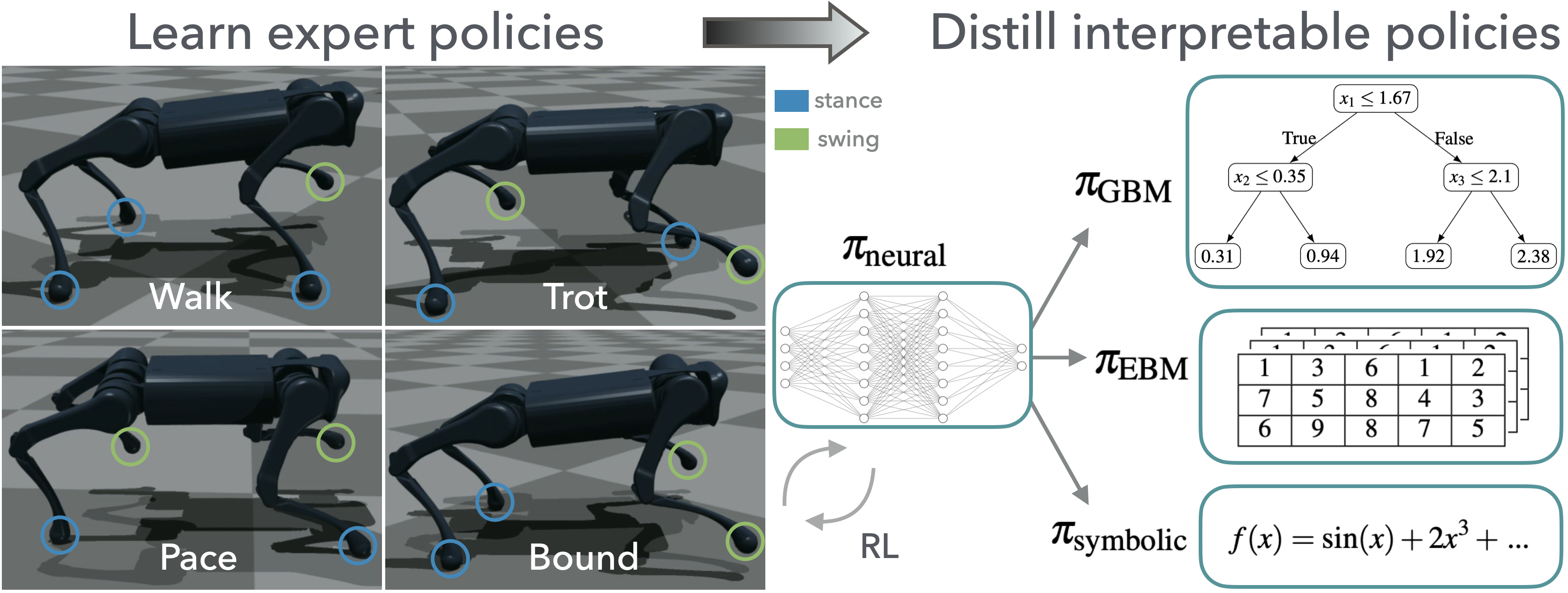
Figure 1: From black-box to glass-box: summary of the proposed framework for distillation of neural network-based RL policies into interpretable policies consisting of GBMs, EBMs, and symbolic policies.

RL for robot locomotion has rapidly matured in capabilities in recent years, ranging from early demonstrations of policy gradients for training simple locomotion policies [8], to the use of animal motion imitation [9], and traversal of challenging terrain [4]. Some previous work has focused on developing modular or hierarchical architectures, both in locomotion [5, 10, 11], and manipulation settings [12, 13, 14], which are intrinsically not as black-box due to their modular structure, however this was mainly done for improving policy performance or learning efficiency – without delivering interpretability insights (except for [12] in manipulation). Notably, [11] evaluates observation importance for efficient learning of locomotion policies, but uses neural policies and thus can only use black-box saliency methods for importance analysis. Additionally, recent work has demonstrated the ability to learn exteroceptive policies, from sparse environment perception [15, 16] to more dense or visual perception [6, 17, 18], further advancing the capabilities of robot locomotion learned via RL – while maintaining the use of neural networks as policies.

Nevertheless, there is a growing need to produce interpretable policies and thus enable more widespread adoption of intelligent legged robots. Explainable RL has recently developed in various directions [3], with policy distillation or extraction becoming increasingly popular: decision trees guided by Q-functions have been distilled from neural policies for simple game environments [19], as well as state machines and list processing programs [20], and decision trees have also been used for evolutionary feature synthesis [21] to provide visualizations and rule-based explanations of simple agent-environment interactions [22]. Moreover, neural RL expert policies have been distilled into decision trees in various domains where interpretability is crucial, such as power system control [23], aircraft separation assurance [24], and sensor-based robot navigation [25].

To address the need for policy interpretability and inspired by previous work on explainable RL, we develop a novel framework for distilling neural network expert locomotion policies trained via RL into more interpretable glass-box policies, as shown in Figure 1. Our main contributions are:

• A novel policy distillation framework incorporating episode-dependent policy alternation to DAgger [26].

• Effective locomotion policies distilled via Gradient Boosting Machines (GBMs) [27], Explainable Boosting Machines (EBMs) [28], and Symbolic Regression [29].

• Interpretability of the observation-action mapping unveiled in the distilled locomotion policies, and the evaluation of their performance in tasks consisting of walking, trotting, pacing, and bounding gaits, providing both global and local explanations of policy actions.

We follow a distillation approach as the interpretable models we use cannot be trained to perform general function approximation parametrically via policy gradients, they are best suited for regression on a supervised dataset. To the best of our knowledge, our work is the first to distill RL locomotion policies into GBMs, EBMs, and symbolic policies.

II Background

II-A Reinforcement Learning for Robot Locomotion

RL is the machine learning paradigm for decision-making or control [30], also known as approximate dynamic programming for solving Markov Decision Processes (MDPs), defined as a tuple $\langle\mathcal{S},\mathcal{A},P(s_{t+1}|s_{t},a_{t}),R\rangle$, where $\mathcal{S}$ is the state space, $\mathcal{A}$ is action space, $P(s_{t+1}|s_{t},a_{t})$ is the transition dynamics, and $R$ is the reward function. We denote a policy $\pi:\mathcal{S}\rightarrow\mathcal{A}$ parametrized by $\theta$ as $\pi_{\theta}$.

The RL objective is to maximize cumulative rewards, and policy gradient algorithms are a popular approach to approximately solve this using differentiable policies $\pi_{\theta}$ such as neural networks, by optimizing an objective of the form:

$$\nabla_{\theta}\mathbb{E}\left[\sum_{t=0}^{T}r_{t}\right]\approx\mathbb{E}\left[\sum_{t=0}^{T}\Psi_{t}\nabla_{\theta}\log\pi_{\theta}(a_{t}|s_{t})\right]$$ (1)

where $\Psi_{t}$ takes different forms depending on the algorithm, such as discounted returns, temporal-difference residual, or a clipped surrogate objective in the case of the popular algorithm Proximal Policy Optimization (PPO) [31], which uses the parameter update $\theta_{k+1}=\arg\max_{\theta}\mathbb{E}_{s,a\sim\pi_{\theta_{k}}}\left[L(s,a,\theta_{k},\theta)\right]$ where $L(s,a,\theta_{k},\theta)$ is a clipped lower bound objective.

In RL for robot locomotion, the MDP state usually includes joint states, velocities, base orientation, velocity, additional terms like feet height, contact states, target velocity, or distance to target, and exteroceptive information if relevant, with actions typically being joint position targets executed by high-frequency low-level joint PD controllers for compliant behavior [4, 5, 11, 15, 6, 18]. Reward functions often combine target tracking, joint state or target smoothness, and other shaping terms for desired gaits. Our approach utilises reward machines that structure reward functions as state machines and extend the MDP state with the reward machine state, enhancing learning efficiency and locomotion robustness [7]. This also aids policy interpretability through the logical rules of reward machine states. See [7] for an in-depth discussion on locomotion reward machines.

II-B Gradient Boosting Machines and Symbolic Regression

Generalized Additive Models (GAMs) are a flexible class of models that extend linear models by allowing non-linear relationships between each predictor and the response variable, while maintaining additivity [32]. The model can be expressed as:

$$g(\mathbb{E}[y])=\beta_{0}+f_{1}(x_{1})+f_{2}(x_{2})+\cdots+f_{p}(x_{p})$$ (2)

where $y$ is the response variable, $g(\cdot)$ is a link function (identity for regression, sigmoid for classification), $x_{i}$ are predictors, $\beta_{0}$ is the intercept, and $f_{i}$ are shape functions.

Gradient Boosting Machines (GBMs) are an ensemble learning technique that builds models sequentially, each new model correcting errors made by the previous ones [27]. A GBM combines weak learner models, typically shallow decision trees, to create a strong predictive model:

$$\hat{y}=\sum_{i=1}^{M}\gamma_{i}h_{i}(x),$$ (3)

where $\hat{y}$ is the predicted response, $h_{i}(x)$ are the weak learner models, $\gamma_{i}$ are the corresponding weights, and $M$ is the number of models.

Explainable Boosting Machines (EBMs) combine the advantages of gradient boosting from GBMs, with the intelligibility of GAMs [28]. Notably, EBM implementations allow for univariate $f_{i}$ and optionally bivariate $f_{i,j}$ shape functions when valuable [33], expanding GAMs by accounting for pairwise interaction terms as:

$$g(\mathbb{E}[y])=\beta_{0}+\sum f_{i}(x_{i})+\sum f_{i,j}(x_{i},x_{j})$$ (4)

where $f_{i}$ and $f_{i,j}$ are essentially learned lookup tables.

Symbolic regression seeks mathematical models that best describe data, differing from traditional regression by not strictly presupposing the model structure [29]. Utilizing genetic algorithms (GAs), symbolic regression evolves expressions using unary and binary operators to minimize an error metric $\mathcal{L}$ over data $D$ as $\min_{f}\mathcal{L}(D,f(x))$ where $f(x)$ is usually a GAM with complexity constraints. This symbolic approach enables the discovery of interpretable models, revealing inherent data patterns [29].

III Methodology

We now present the methodology used in this work. Our framework consists of (i) training of RL experts as neural policies, and (ii) distillation of the neural policies into interpretable policies. We note that we follow this process because the types of interpretable policies we use are not suitable for gradient-based optimization of policy parameters, which is a requirement of policy gradient RL methods. Moreover and noticeably, the neural policies used in previous locomotion work are not particularly deep, usually having 2 to 5 hidden layers [4, 5, 15], and hence the limited expressiveness of these networks suggests that the observation-action mapping learned via RL can be distilled into simpler forms, such as decision trees or additive models, which motivates our work.

TABLE I: Top 3 Observations by Importance for Each Joint Type Action From Distilled Gradient Boosting Machine Policies Based on Feature and Permutation Importance for 4 Different Gaits

Gait	Joint Type	1st Feature	2nd Feature	3rd Feature
Feature Importance
Walk	Hip	Prev Action Hip	RM State	RM Iters, DoF Pos or Prev Action Calf, Height Foot
	Thigh	Prev Action Thigh	RM State, RM Iters, DoF Pos Thigh	Prev Action Hip, Command X
	Calf	Prev Action Hip or Calf	RM Iters, Prev Action Hip or Calf	Prev Action Hip or Thigh
Trot	Hip	Prev Action Hip	RM State, RM Iters, Prev Action Hip or Thigh	RM Iters, Prev Action Calf
	Thigh	Prev Action Hip or Thigh	RM Iters, Command X, Prev Action Thigh or Calf	RM Iters, RM State, Foot Height
	Calf	Prev Action Hip or Calf	Prev Action Calf or Hip, RM State	Prev Action Hip or Thigh
Pace	Hip	Prev Action Hip, Dof Vel Hip, RM Iters, Foot Height	DoF Pos or Vel Thigh, RM State, RM Iters	Prev Action Hip, Foot Height, DoF Vel Calf
	Thigh	Prev Action Hip, RM Iters, Foot Height	Foot Height, Prev Action Hip	DoF Vel Hip or Thigh, Command X
	Calf	Prev Action Hip or Thigh	Prev Action Thigh or Calf, RM Iters, Foot Height	RM Iters, DoF Pos or Vel Thigh
Bound	Hip	Prev Action Hip	Prev Action Hip or Thigh	Prev Action Calf, Base Lin Vel Z
	Thigh	Prev Action Thigh	Prev Action Thigh or Calf, RM Iters	Foot Height, Command X, Prev Action Hip or Calf
	Calf	Prev Action Calf or Hip	Prev Action Calf or Hip	Prev Action Hip or Thigh
Permutation Importance
Walk	Hip	Prev Action Hip	RM State, Foot Height	RM Iters, RM State, Prev Action Calf
	Thigh	Thigh Prev Action	RM State, RM Iters, Command X	Prev Action Hip, Command X
	Calf	Prev Action Hip or Calf	Prev Action Calf or Hip, RM State	Prev Action Hip or Thigh
Trot	Hip	Prev Action Hip	RM State, RM Iters, Prev Action Hip or Calf	RM Iters, Prev Action Thigh or Calf
	Thigh	Prev Action Hip or Thigh	RM Iters, Command X, Prev Action Thigh or Calf	RM Iters, RM State, Foot Height
	Calf	Prev Action Hip or Calf	Prev Action Calf or Hip, RM State	Prev Action Hip or Thigh
Pace	Hip	Foot Height, Prev Action Hip, RM Iters	Prev Action Hip, DoF Pos Hip, RM Iters, DoF Vel Calf	Prev Action Hip or Thigh, DoF Vel Thigh, RM State
	Thigh	Prev Action Hip, RM Iters, Foot Height	Foot Height, Prev Action Hip	DoF Vel Hip or Thigh, Command X
	Calf	Prev Action Hip or Thigh	Prev Action Thigh or Calf, RM Iters, Foot Height	RM Iters, DoF Pos or Vel Thigh
Bound	Hip	Prev Action Hip	Prev Action Hip or Thigh	Prev Action Calf, RM State
	Thigh	Prev Action Thigh	Command X, Prev Action Hip	RM State, RM Iters, Prev Action Thigh or Calf
	Calf	Prev Action Calf or Hip	Prev Action Calf or Hip, Base Lin Vel Z	Prev Action Hip or Calf

III-A Training Reinforcement Learning Expert Policies

In general, RL algorithms require $\pi_{\theta}$ to be differentiable, and therefore we cannot easily train GBMs, EBMs, or symbolic policies directly via RL as these are not directly amenable for gradient-based optimization. Thus, we use neural networks for our experts. We train expert policies for the following tasks or gaits: walk, trot, pace, and bound. To obtain our neural expert policies, we use the PPO algorithm in IsaacGym simulations. As previously mentioned, we build on top of [7], but we note that our approach is agnostic to the specific details regarding the RL methodology used to train the neural experts. The logical propositions used for defining the reward machines for each gait can be found in [7]. All gaits use the same base observations and only differ in their reward machine states. Full observation lists are in Figure 11. A learned state estimator is used for base velocity and feet contact forces [7], but other alternatives could be used.

We use the Unitree A1 quadruped robot for our experiments. Each expert policy is trained with randomized forward velocity commands in the range $[-1,1]$ m/s and yaw rate commands in $[-1,1]$ rad/s. The control frequency is 50Hz, with joint PD controllers set at $P=20$ and $D=0.5$ as [7]. We train the expert policy for each gait for 1.5k PPO updates [31] using 1024 parallel environments, which equates to approximately 205 hours of simulated time used to train each expert – substantially less than previous work [15], highlighting the sample efficiency of using reward machines.

III-B Distilling Interpretable Locomotion Policies

In essence, our distillation process is an imitation learning problem, where the expert policies have been trained via RL. Therefore, it is subject to the distribution shift found in vanilla behavioural cloning. To address this, we use the Dataset Aggregation method (DAgger) [26]. However, instead of directly combining pure expert and imitation policy rollouts in the supervised dataset, we modify DAgger to use episode-dependent alternation of actions given by the expert and distilled policies, as shown in Algorithm 1. We experimentally found that without this modification policy performance was poor, yielding unstable gaits (this might be addressable by increasing $max\_episodes$ substantially, but it could make distillation prohibitively expensive).

The alternation ratio $1/n$ determines how often the expert actions are used during rollouts, with $n$ increasing during the distillation process as a curriculum. This modification is well motivated for robot control settings with feedback policies, as the action alternation leads to a more graceful trajectory distribution shift in the data used to train the distilled policy.

We used $t=1000$, corresponding to only 10 minutes as the total simulated time in the distillation dataset $D$ for each gait. Specifically, policies are trained with $max\_episodes=30$ alternating linear velocity commands in $[0,0.25,0.5,0.75]$ and only updating $n$ after cycling through all the velocity commands (i.e. $n_{f}=4$), thus the lowest alternation ratio found in the datasets used for distillation is $1/8$.

Using Algorithm 1, in step 19 we distill three types of interpretable locomotion policies for each gait: GBMs, EBMs, and symbolic expressions, leaving 20% of $D$ as test set. We leverage efficient implementations from [34] for GBMs, from [33] for EBMs, and from [29] for Symbolic Regression, with default hyperparameters for each as they are optimized for robust performance. For Symbolic Regression, we use the unary operators $[\sin(\cdot),\tanh(\cdot),\cdot^{2},\cdot^{3}]$, and binary operators $[\cdot+\cdot,\cdot-\cdot,\cdot\times\cdot]$ with maximum operator complexity 4 and overall complexity 90, for 20 iterations per distillation.

Algorithm 1 DAgger with Curriculum of Episode-Dependent Alternation of Expert and Distilled Policy Actions

1:Initialize dataset $D\leftarrow\emptyset$

2:Initialize distilled policy $\pi_{\text{distilled}}$ randomly

3:Initialize pre-trained expert policy $\pi_{\text{expert}}$

4:Set frequency parameter $n_{f}$

5:Set maximum episodes $max\_episodes$

6:for $episode=1$ to $max\_episodes$ do

7:     Set $n\leftarrow\max(1,\lceil episode/n_{f}\rceil)$

8:     Initialize episode trajectory $\tau\leftarrow\emptyset$

9:     for each step $t$ of the episode do

10:         if $t\mod n=0$ then

11:              Execute action $a_{t}\leftarrow\pi_{\text{expert}}(s_{t})$ $\triangleright$ Use expert policy every $1/n$ steps

12:         else

13:              Execute action $a_{t}\leftarrow\pi_{\text{distilled}}(s_{t})$ $\triangleright$ Use distilled policy otherwise

14:         end if

15:         Observe new state $s_{t+1}$ and reward $r_{t}$

16:         Append $(s_{t},a_{t},s_{t+1},r_{t})$ to $\tau$

17:     end for

18:     Aggregate dataset $D\leftarrow D\cup\{(s_{t},\pi_{\text{expert}}(s_{t}))\,|\,(s_{t},\cdot,\cdot,\cdot)\in\tau\}$

19:     Update $\pi_{\text{distilled}}$ by supervised learning on $D$

20:end for

IV RESULTS

We present the results of the GBM, EBM, and symbolic policies across various gaits: walking, trotting, pacing, and bounding. A comprehensive data analysis is conducted to thoroughly delineate both the performance and interpretability of these policies.

IV-A Performance of Distilled Policies

We evaluate the performance of all distilled policies after termination of Algorithm 1. We do this from the perspective of regression performance and task performance during policy rollouts in our simulated environment.

TABLE II: Comparison of $R^{2}$ Scores on Test Sets Across Different Gaits

Model Type	Walk	Trot	Pace	Bound
GBM	0.9705	0.9863	0.9752	0.9537
EBM	0.9787	0.9906	0.9819	0.9637
Symbolic	0.6811	0.7334	0.7331	0.6564

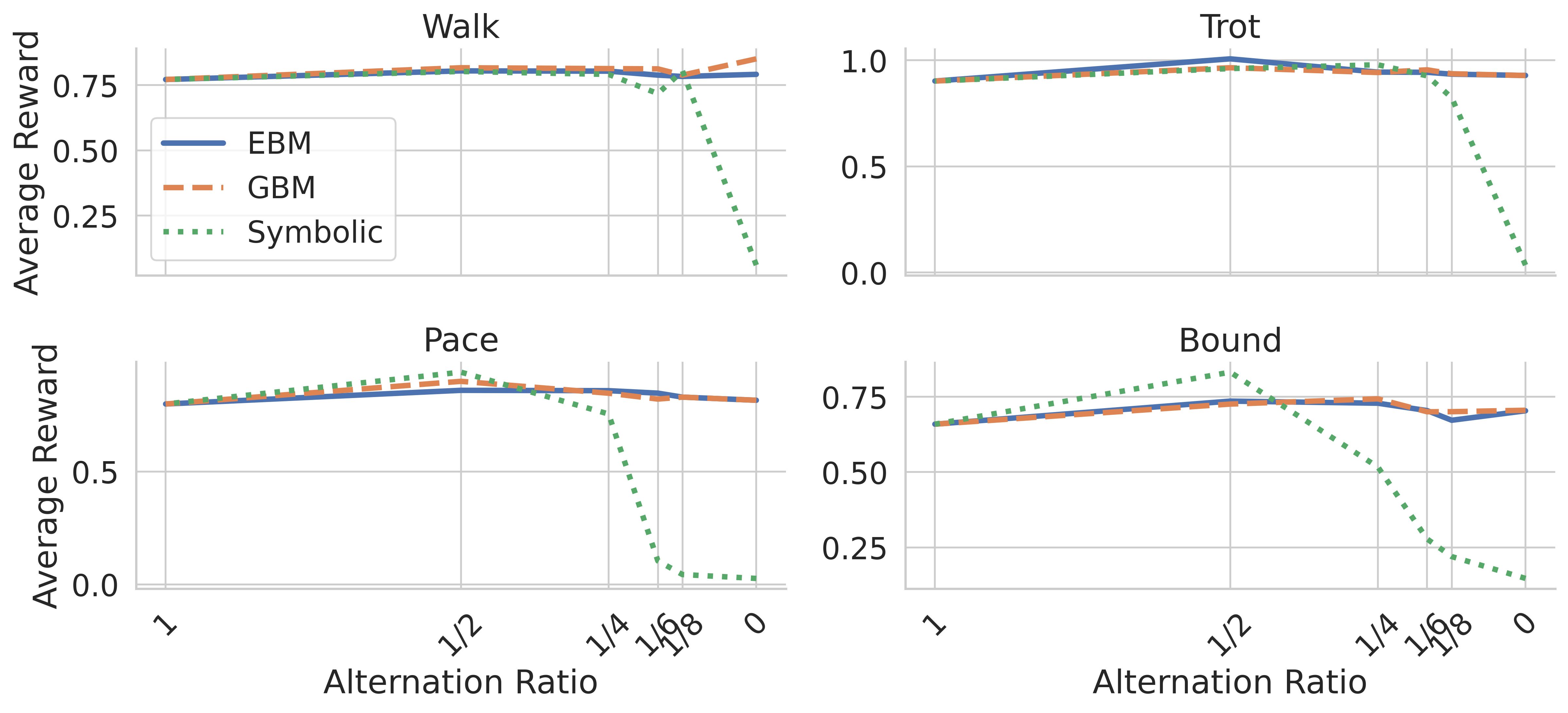
Figure 2: Average episodic performance of distilled policies for all gaits tested using various alternation ratios. Note that alternation ratio of 1 means only the neural RL expert is used, 0 means only the distilled policy is used.

The regression performance of each method at imitating the corresponding expert policies for each gait quantified by the $R^{2}$ score is shown in Table II. We note how EBMs and GBMs perform similarly for all gaits, with EBMs performing best, and symbolic policies performing worst. Performance of the symbolic policy might be improved if the genetic algorithm were to be run for more iterations, however these are significantly time-consuming to run and we present results of the best performing unary and binary operators we found after testing various combinations.

We evaluate each distilled policy upon termination of Algorithm 1 in simulation with 26 parallel environments using various alternation ratios and provide average episodic rewards in Figure 2. These results provide several relevant insights. First, GBM and EBM policies generally maintain performance regardless of the alternation ratio used, whereas symbolic policies yield degraded performance as the neural RL expert is used less often, which is aligned with scores in Table II. Second, it shall be noted that for all gaits there is at least one configuration that outperforms the RL expert (i.e. alternation ratio of 1). Notably, when used strictly by themselves (i.e. alternation ratio 0), the GBM walk policy outperforms the neural RL expert by over 10%, the EBM and GBM trot policies by 3%, the EBM and GBM pace policies by 2%, and the EBM and GBM bound policies by nearly 7%. This is usually due to better linear and angular velocity reward performance. The performance of the symbolic policies generally matches and sometimes outperforms alternatives when alternated with RL experts (by 12% for pace and 10% for bound with alternation ratio $1/2$), but decays rapidly for alternation ratios below $1/6$ for walk and trot, and below $1/4$ for pace and bound, yielding unusable policies in isolation. It shall be noted standalone evaluations of distilled policies (i.e. alternation ratio of 0) constitute a setting that was never seen in the distillation training data.

Additionally, we provide a visual depiction of the gait sequences when testing the distilled policies running in isolation (i.e. alternation ratio 0), with GBM policies shown in Figure 3, EBM policies in Figure 4, and symbolic policies in Figure 5. It shall be noted how GBM and EBM policies yield visually similar gaits, whereas the symbolic policy yields visibly worse gaits, which is aligned with the results in Figure 2 and Table II. Tested in isolation, only GBM and EBM policies yielded stable gaits that could run for the full duration of the test episodes, whereas symbolic gaits were not able to sustain more than a couple of gait cycles.

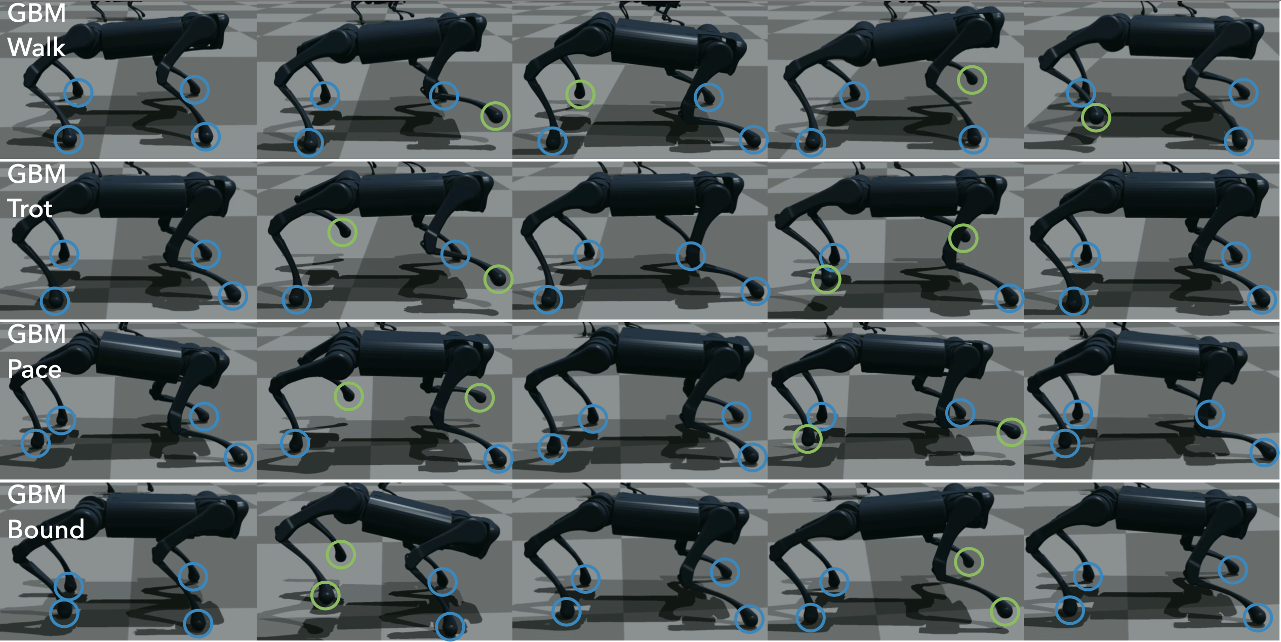
Figure 3: Gait sequences for walk, trot, pace, and bound GBM policies.

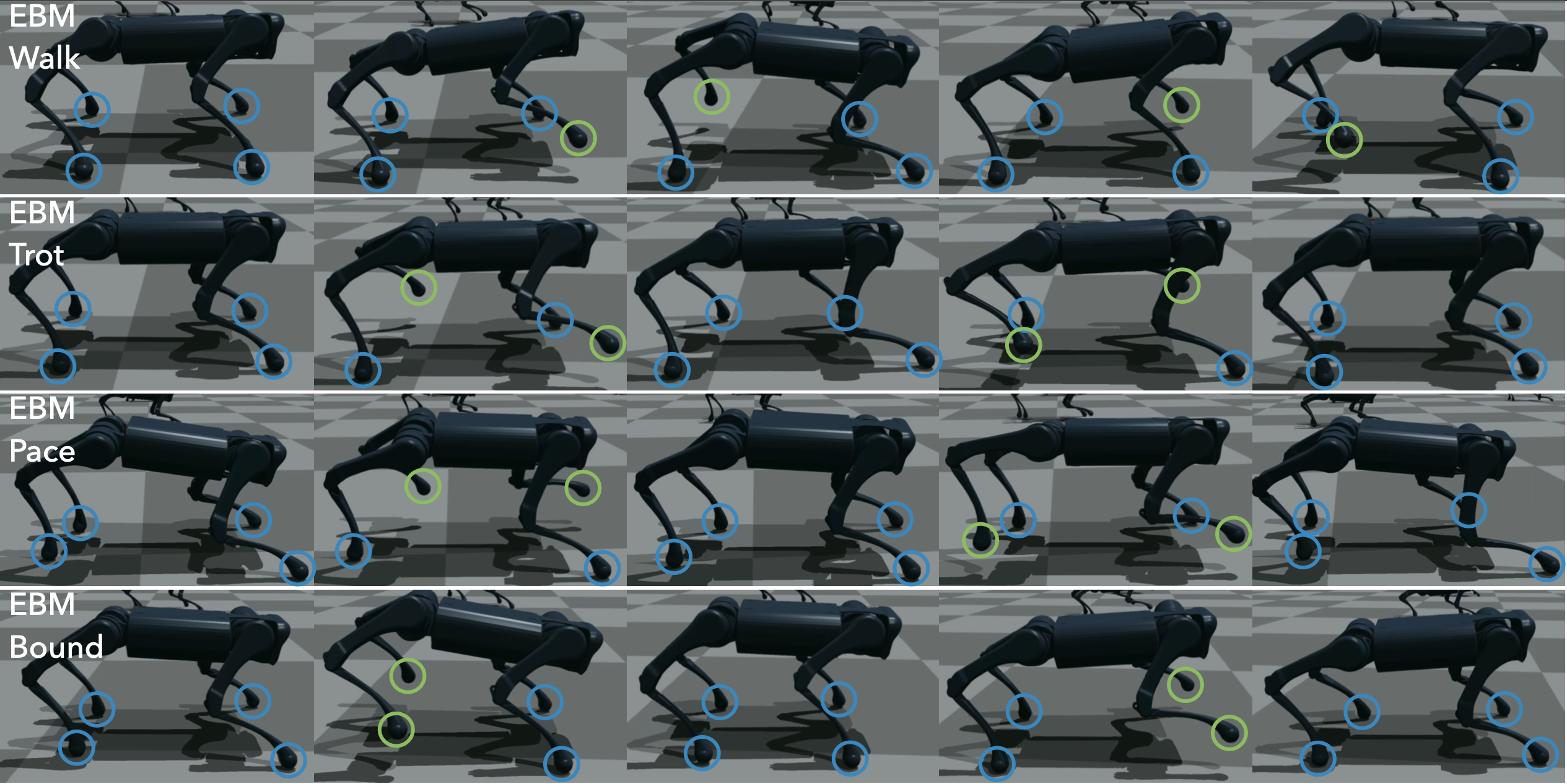
Figure 4: Gait sequences for walk, trot, pace, and bound EBM policies.

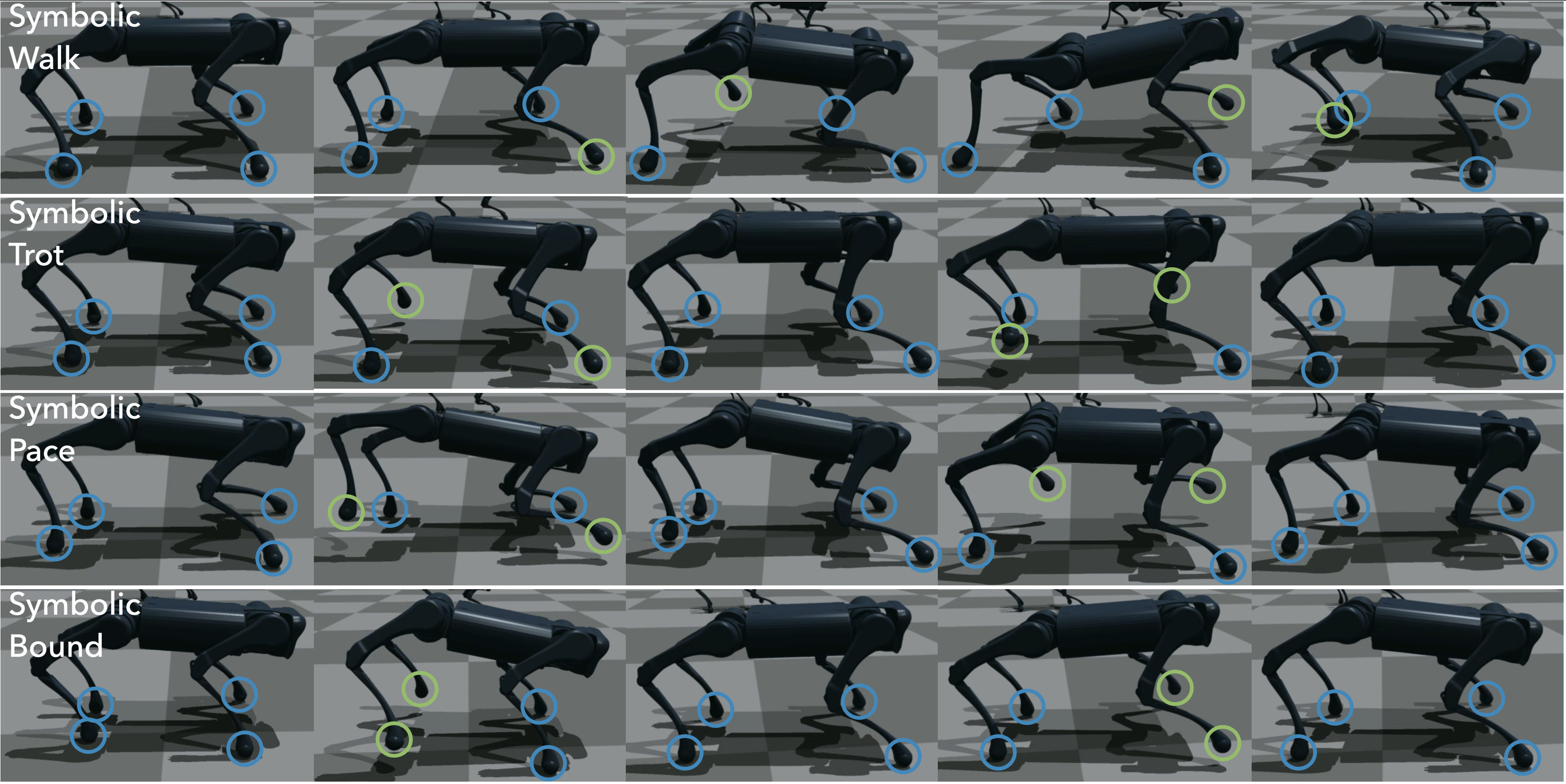
Figure 5: Gait sequences for walk, trot, pace, and bound symbolic policies.

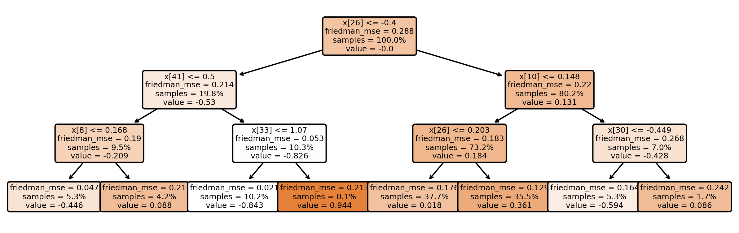
Figure 6: Example of one of the decision trees used as weak learners in the distilled GBM walk policy for Front Left Hip.

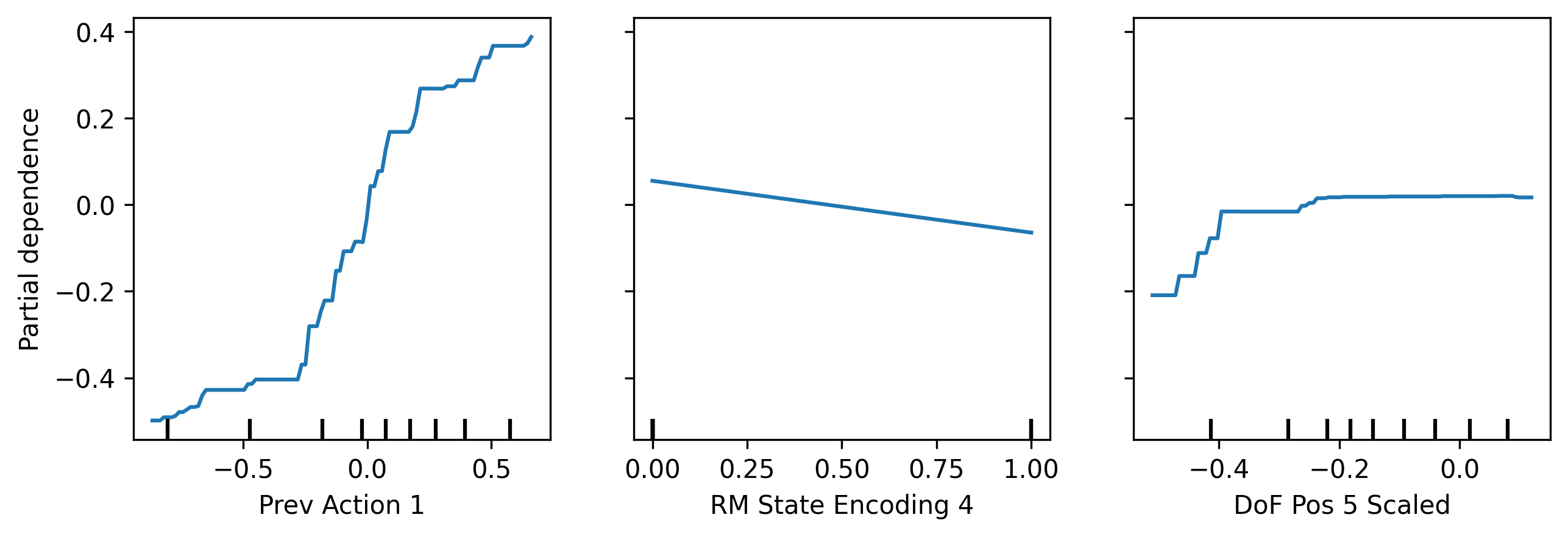
Figure 7: Partial dependence to top 3 observations by feature importance in distilled GBM walk policy for Front Left Hip.

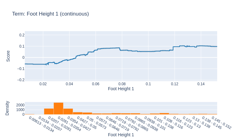
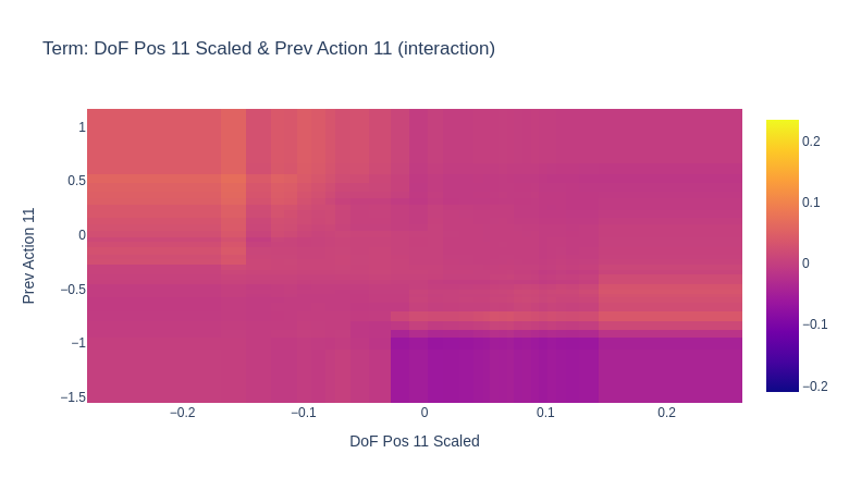
Figure 8: Example global explanations (top: single observation, bottom: interacting observation pair) for EBM trot policy actions for Front Left Hip joint.

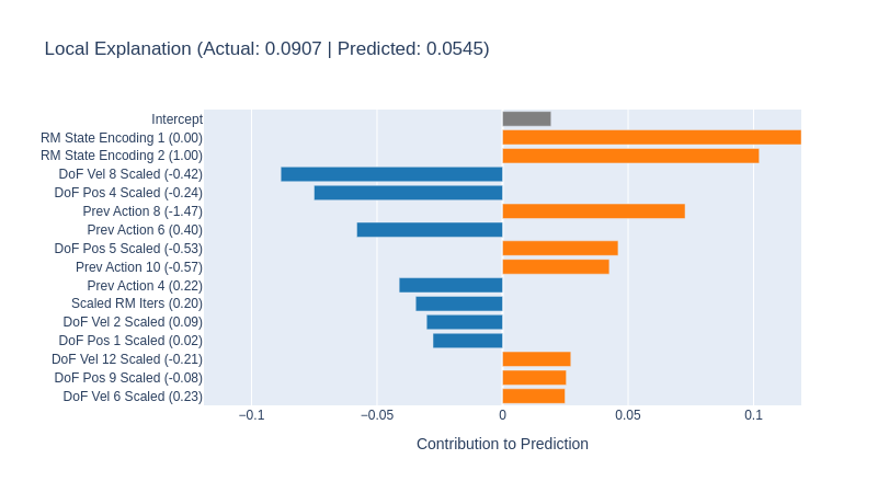
Figure 9: Example local explanation for EBM pace policy action for Front Left Hip joint from an evaluation rollout.

IV-B Interpretability of Distilled Policies

With regards to GBMs, we use two different methods for policy interpretability: feature importance and permutation importance [34], which quantify importance based on decision tree branches and the effect of permutations respectively. We provide the importance maps for all gaits in Figure 11, and we also provide a summary of those results based on joint type (hip, thigh, calf) for the top 3 observations for each method and gait in Table I. We note how generally the differences between importance methods is found on the third or second most relevant feature, mostly agreeing on the top feature for all joint types. These results provide a decomposition of the observations relevant for producing the behaviour corresponding to each gait for each joint level in quadruped locomotion. GBMs allow for some global explanations via inspection of decision trees or partial dependence plots as shown in Figures 6 and 7 from which counterfactual information could be obtained for certification purposes, e.g. what value should an observation have taken for an action output to be beyond a certain level.

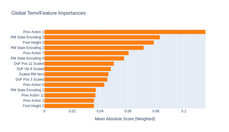
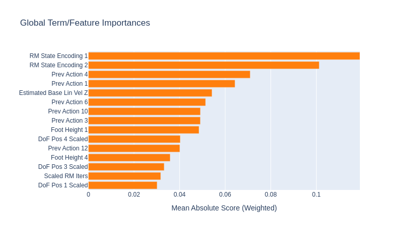
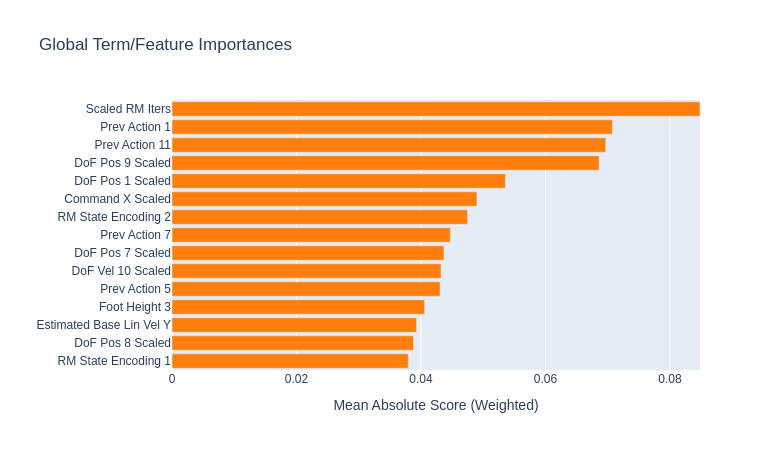
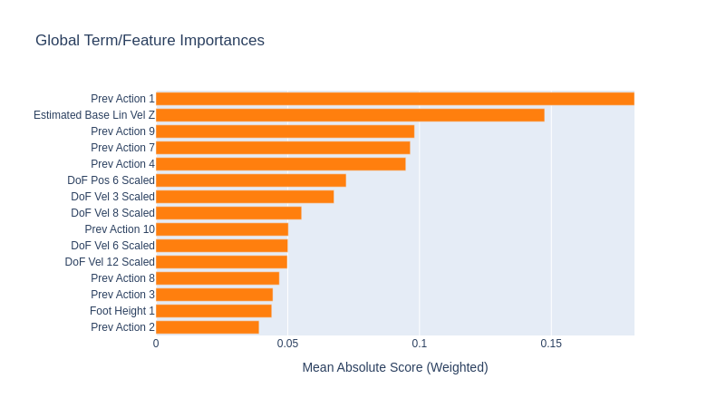
Figure 10: Global importances for EBM policies for walk, trot, pace, and bound (respectively, top to bottom) for Front Left Hip joint actions.

Regarding EBMs, since they are modified GAMs, we can easily obtain the global importance of each term without additional models or computation, consisting of single and pairwise feature terms in Equation 4. We provide the global importances of each term for distilled EBM policies in Figure 10. As detailed in [33], EBMs are highly intelligible because the contribution of each term to the final prediction can be visualized and understood by plotting $f_{i}$ or $f_{i,j}$, providing global explanations of policy behaviour. Examples of such global explanations are presented in Figure 8, which show the mapping learned by the policy for a specific observation or observation pair. We note how EBM top important features are different from GBM top important features, summarized in Table I, highlighting how observation importance for the same task varies depending on model architecture.

Figure 8 shows how trot policy actions for the Front Left Hip joint are influenced by its foot height, as well as the pairwise interaction of the terms for previous action and joint position of the Hind Right Thigh. We note how this pairwise interaction map resembles a signed “exclusive or” operation, with near zero contribution to target joint angle in general, except for positive contributions when the previous action is positive and the joint position is negative, and negative contributions when the previous action is negative and the joint position is positive. EBMs also allow for local explanations, i.e. explaining the action corresponding to a specific input observation, as show in Figure 9. We argue this is particularly useful for safety certification or investigation purposes in the presence of malfunctions. Lastly, symbolic policies are interpretable in the sense that they constitute analytical expressions, and importance could be studied using partial derivatives, but we omit this due to their under-performance and for brevity (each policy has up to 90 terms).

V CONCLUSION

This work presents a novel approach for distilling neural network-based RL locomotion policies into interpretable ones, consisting of GBMs, EBMs, and symbolic policies for four gaits: walking, trotting, pacing, and bounding. Following the proposed methods, we conducted a thorough analysis of the performance and interpretability of distilled policies. Our results show that interpretable policies can be efficiently extracted from neural locomotion policies, which reveal valuable insights into the behaviour of RL locomotion policies and enable global and local explanations of the learned observation-action mapping, without compromising performance in the case of GBMs and EBMs.

To the best of our knowledge, our work is the first to demonstrate that interpretable models can be used as policies for robot locomotion, and this work contributes to increased interpretability of RL locomotion policies. Future research directions include exploring the scalability of our approach to exteroceptive policies, incorporating uncertainty estimates, and extending our methodology to robot manipulation. We hope this work contributes towards enabling a widespread and trustworthy adoption of autonomous robots.

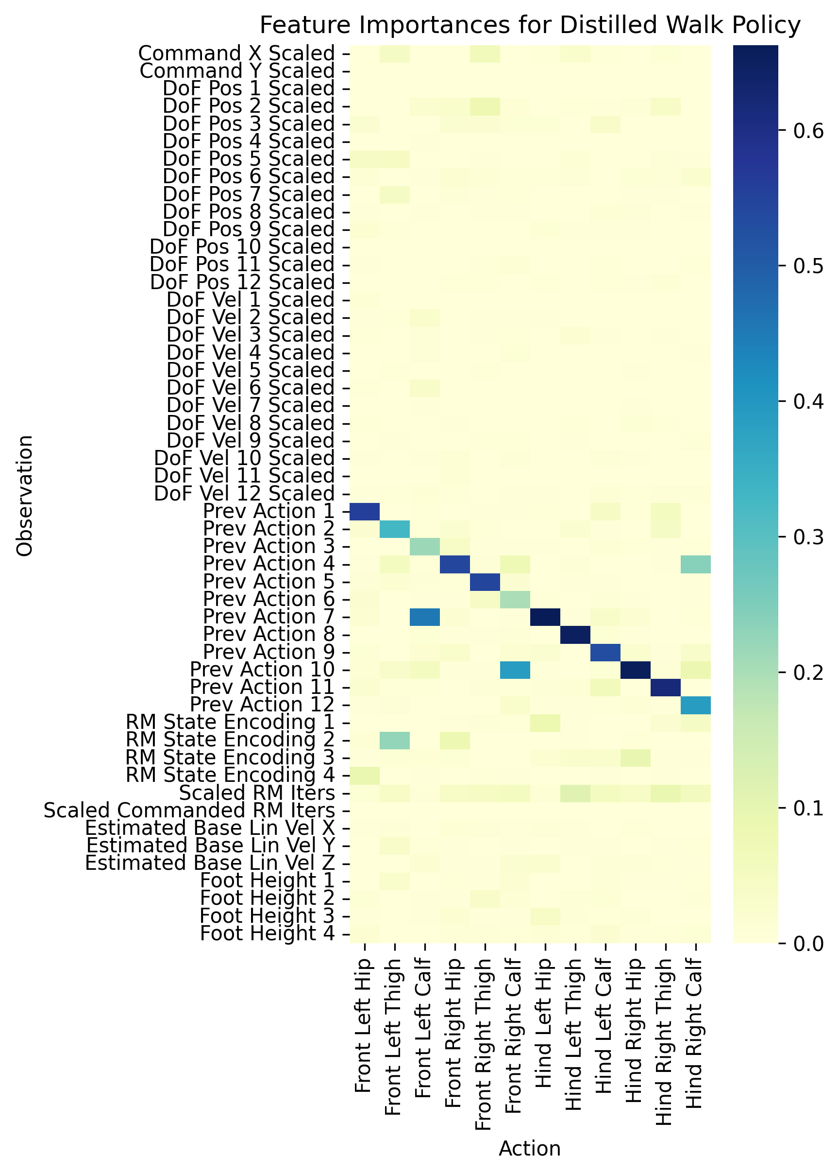
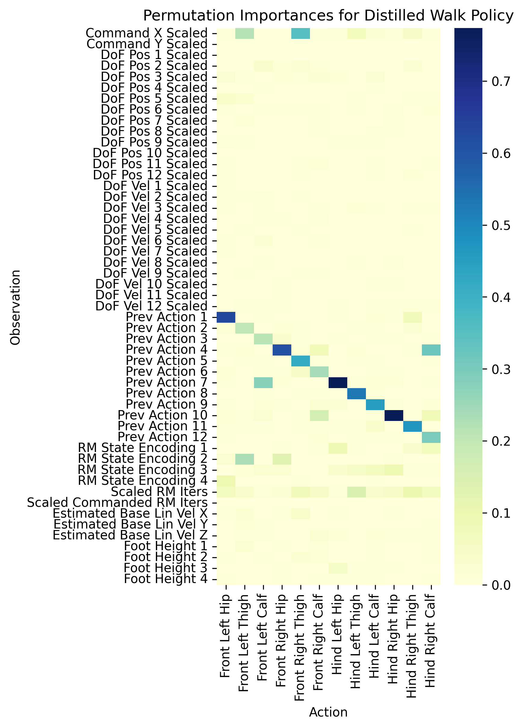
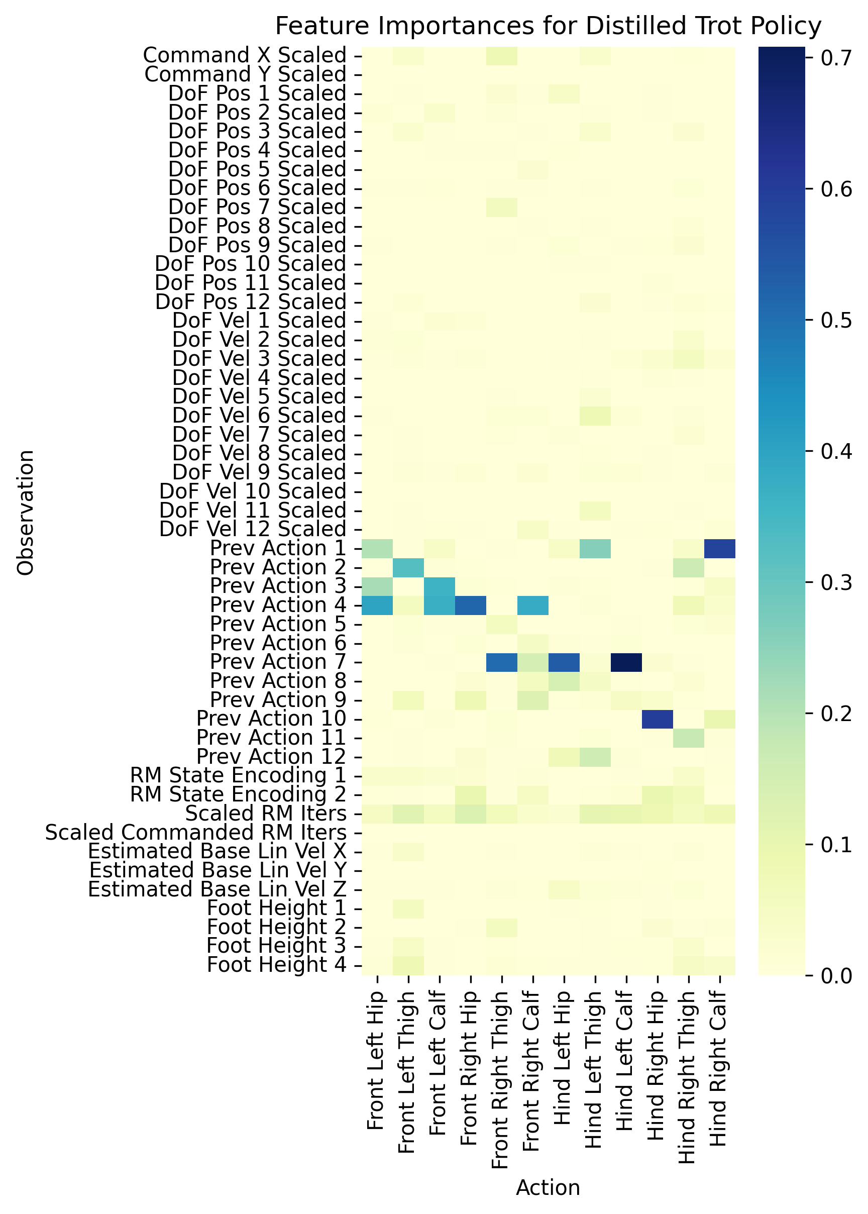
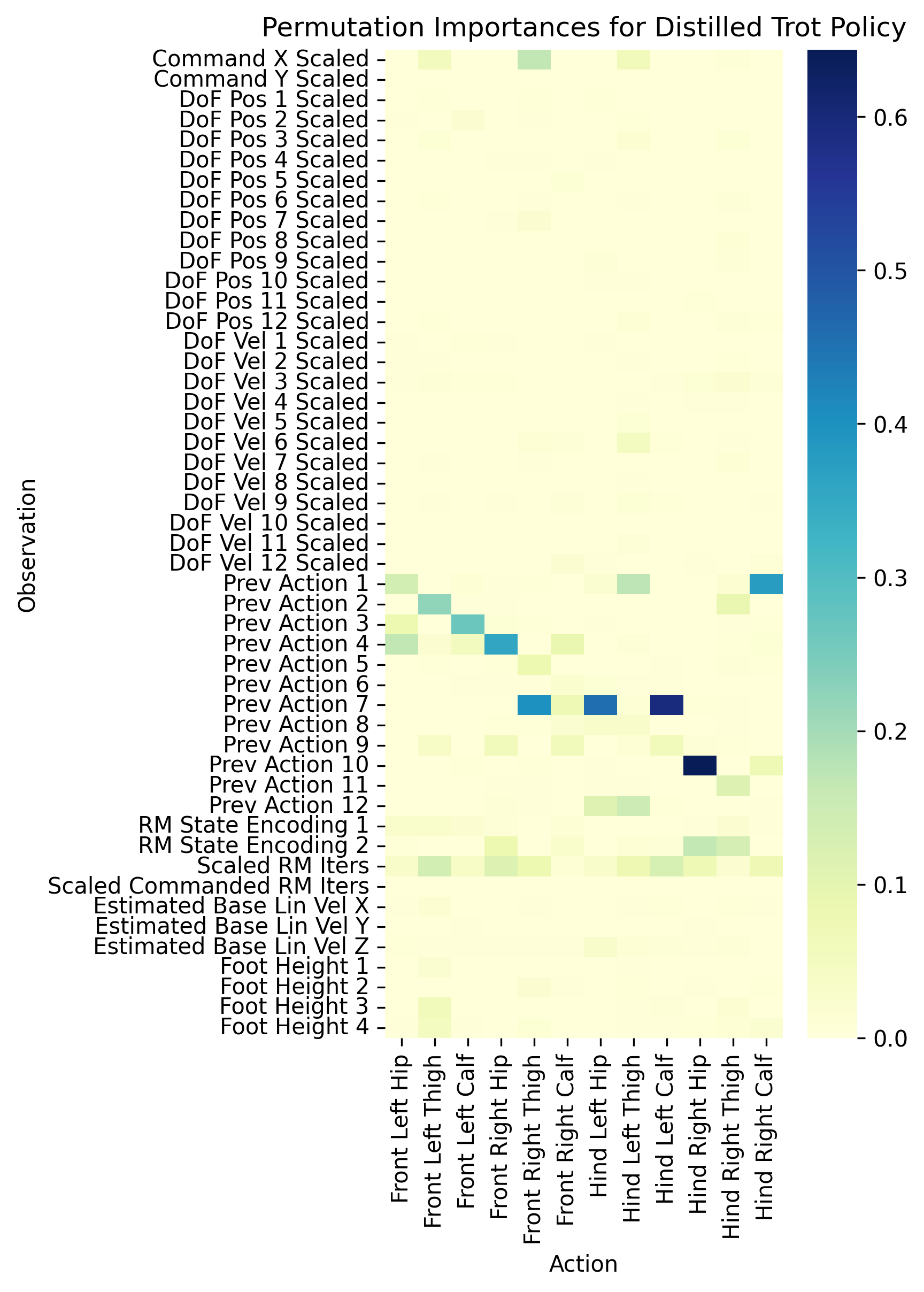
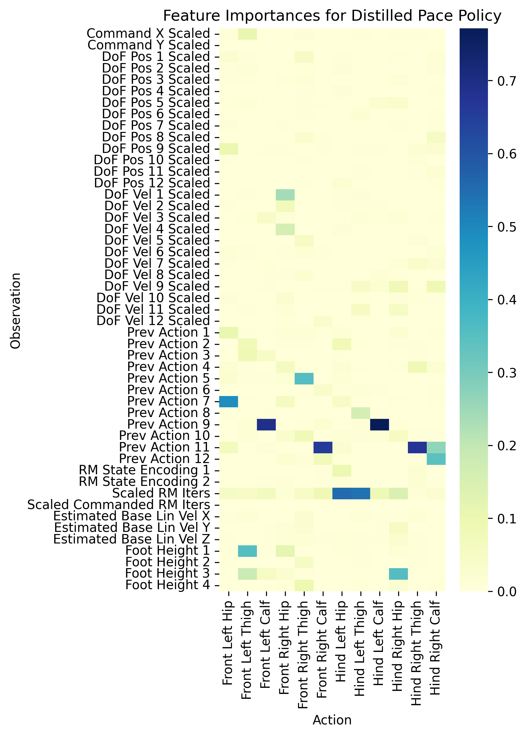
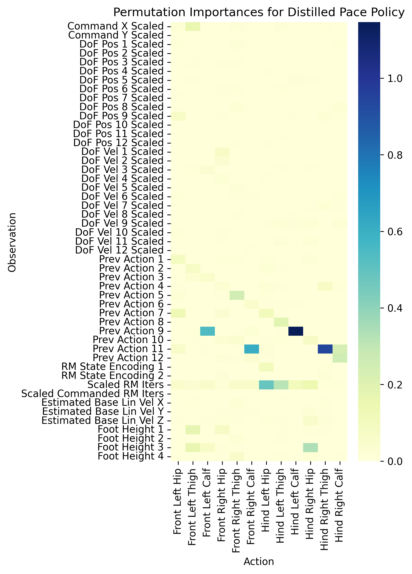
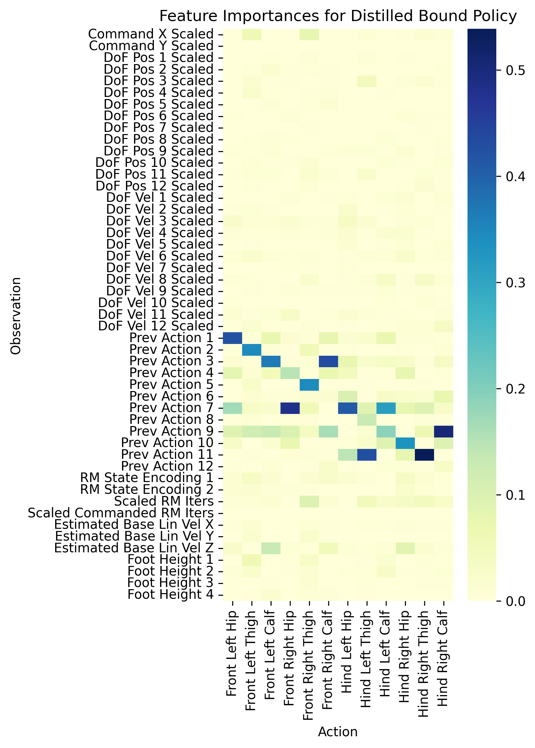
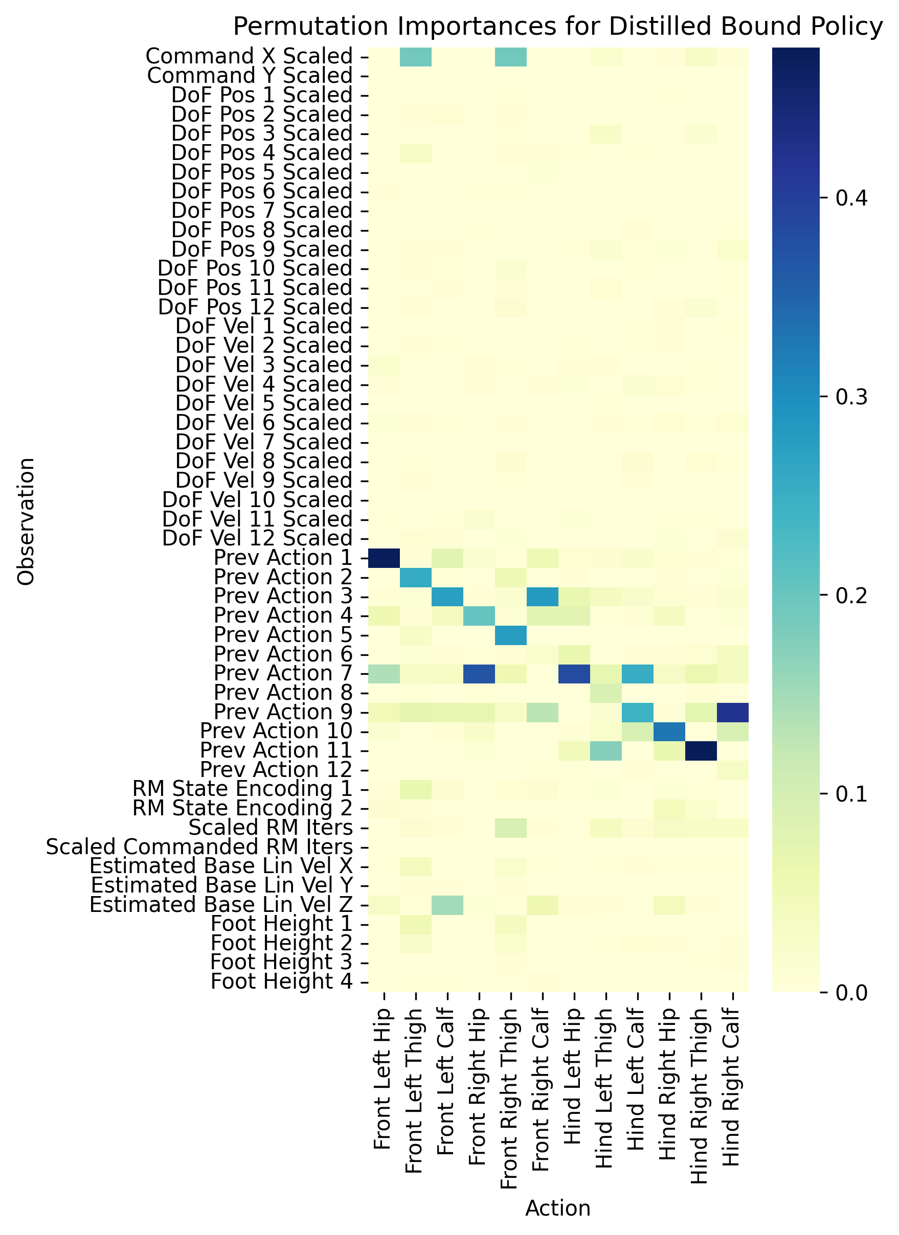
Figure 11: Observation importances for GBM policies computed using two distinct methods: feature importance and permutation importance [34].

References

- [1] D. Gunning, M. Stefik, J. Choi, T. Miller, S. Stumpf, and G.-Z. Yang, “Xai—explainable artificial intelligence,” Science Robotics, vol. 4, no. 37, p. eaay7120, 2019.
- [2] T. Sakai and T. Nagai, “Explainable autonomous robots: a survey and perspective,” Advanced Robotics, vol. 36, no. 5-6, pp. 219–238, 2022.
- [3] S. Milani, N. Topin, M. Veloso, and F. Fang, “Explainable reinforcement learning: A survey and comparative review,” ACM Computing Surveys, 2023.
- [4] J. Lee, J. Hwangbo, L. Wellhausen, V. Koltun, and M. Hutter, “Learning quadrupedal locomotion over challenging terrain,” Science Robotics, vol. 5, no. 47, p. eabc5986, 2020.
- [5] C. Yang, K. Yuan, Q. Zhu, W. Yu, and Z. Li, “Multi-expert learning of adaptive legged locomotion,” Science Robotics, vol. 5, no. 49, p. eabb2174, 2020.
- [6] T. Miki, J. Lee, J. Hwangbo, L. Wellhausen, V. Koltun, and M. Hutter, “Learning robust perceptive locomotion for quadrupedal robots in the wild,” Science Robotics, vol. 7, no. 62, p. eabk2822, 2022.
- [7] D. DeFazio, Y. Hayamizu, and S. Zhang, “Learning quadruped locomotion policies using logical rules,” arXiv:2107.10969, 2024.
- [8] N. Kohl and P. Stone, “Policy gradient reinforcement learning for fast quadrupedal locomotion,” in IEEE International Conference on Robotics and Automation, 2004. Proceedings. ICRA’04. 2004, vol. 3. IEEE, 2004, pp. 2619–2624.
- [9] X. B. Peng, E. Coumans, T. Zhang, T.-W. Lee, J. Tan, and S. Levine, “Learning agile robotic locomotion skills by imitating animals,” arXiv preprint arXiv:2004.00784, 2020.
- [10] K. Yuan, N. Sajid, K. Friston, and Z. Li, “Hierarchical generative modelling for autonomous robots,” Nature Machine Intelligence, vol. 5, no. 12, pp. 1402–1414, 2023.
- [11] W. Yu, C. Yang, C. McGreavy, E. Triantafyllidis, G. Bellegarda, M. Shafiee, A. J. Ijspeert, and Z. Li, “Identifying important sensory feedback for learning locomotion skills,” Nature Machine Intelligence, vol. 5, no. 8, pp. 919–932, 2023.
- [12] B. Beyret, A. Shafti, and A. A. Faisal, “Dot-to-dot: Explainable hierarchical reinforcement learning for robotic manipulation,” in 2019 IEEE/RSJ International Conference on intelligent robots and systems (IROS). IEEE, 2019, pp. 5014–5019.
- [13] E. Triantafyllidis, F. Acero, Z. Liu, and Z. Li, “Hybrid hierarchical learning for solving complex sequential tasks using the robotic manipulation network roman,” Nature Machine Intelligence, vol. 5, no. 9, pp. 991–1005, 2023.
- [14] W. Hu, F. Acero, E. Triantafyllidis, Z. Liu, and Z. Li, “Modular neural network policies for learning in-flight object catching with a robot hand-arm system,” in 2023 IEEE/RSJ International Conference on Intelligent Robots and Systems (IROS). IEEE, 2023, pp. 944–951.
- [15] F. Acero, K. Yuan, and Z. Li, “Learning perceptual locomotion on uneven terrains using sparse visual observations,” IEEE Robotics and Automation Letters, vol. 7, no. 4, pp. 8611–8618, 2022.
- [16] Z. Liu, F. Acero, and Z. Li, “Learning vision-guided dynamic locomotion over challenging terrains,” arXiv preprint arXiv:2109.04322, 2021.
- [17] W. Yu, D. Jain, A. Escontrela, A. Iscen, P. Xu, E. Coumans, S. Ha, J. Tan, and T. Zhang, “Visual-locomotion: Learning to walk on complex terrains with vision,” in 5th Annual Conference on Robot Learning, 2021.
- [18] A. Loquercio, A. Kumar, and J. Malik, “Learning visual locomotion with cross-modal supervision,” in 2023 IEEE International Conference on Robotics and Automation (ICRA). IEEE, 2023, pp. 7295–7302.
- [19] O. Bastani, Y. Pu, and A. Solar-Lezama, “Verifiable reinforcement learning via policy extraction,” Advances in neural information processing systems, vol. 31, 2018.
- [20] O. Bastani, J. P. Inala, and A. Solar-Lezama, “Interpretable, verifiable, and robust reinforcement learning via program synthesis,” in International Workshop on Extending Explainable AI Beyond Deep Models and Classifiers. Springer, 2020, pp. 207–228.
- [21] H. Zhang, A. Zhou, and X. Lin, “Interpretable policy derivation for reinforcement learning based on evolutionary feature synthesis,” Complex & Intelligent Systems, vol. 6, pp. 741–753, 2020.
- [22] T. Bewley and J. Lawry, “Tripletree: A versatile interpretable representation of black box agents and their environments,” in Proceedings of the AAAI Conference on Artificial Intelligence, vol. 35, no. 13, 2021, pp. 11 415–11 422.
- [23] Y. Dai, Q. Chen, J. Zhang, X. Wang, Y. Chen, T. Gao, P. Xu, S. Chen, S. Liao, H. Jiang et al., “Enhanced oblique decision tree enabled policy extraction for deep reinforcement learning in power system emergency control,” Electric Power Systems Research, vol. 209, p. 107932, 2022.
- [24] W. Guo and P. Wei, “Explainable deep reinforcement learning for aircraft separation assurance,” in 2022 IEEE/AIAA 41st Digital Avionics Systems Conference (DASC). IEEE, 2022, pp. 1–10.
- [25] A. M. Roth, J. Liang, and D. Manocha, “Xai-n: Sensor-based robot navigation using expert policies and decision trees,” in 2021 IEEE/RSJ International Conference on Intelligent Robots and Systems (IROS). IEEE, 2021, pp. 2053–2060.
- [26] S. Ross, G. Gordon, and D. Bagnell, “A reduction of imitation learning and structured prediction to no-regret online learning,” in Proceedings of the fourteenth international conference on artificial intelligence and statistics. JMLR Workshop and Conference Proceedings, 2011, pp. 627–635.
- [27] J. H. Friedman, “Greedy function approximation: a gradient boosting machine,” Annals of statistics, pp. 1189–1232, 2001.
- [28] Y. Lou, R. Caruana, and J. Gehrke, “Intelligible models for classification and regression,” in Proceedings of the 18th ACM SIGKDD International Conference on Knowledge Discovery and Data Mining, 2012, pp. 150–158.
- [29] M. Cranmer, “Interpretable machine learning for science with pysr and symbolicregression.jl,” arXiv preprint arXiv:2305.01582, 2023.
- [30] R. S. Sutton and A. G. Barto, Reinforcement Learning: An Introduction, 2nd ed. The MIT Press, 2018. [Online]. Available: http://incompleteideas.net/book/the-book-2nd.html
- [31] J. Schulman, F. Wolski, P. Dhariwal, A. Radford, and O. Klimov, “Proximal policy optimization algorithms,” arXiv preprint arXiv:1707.06347, 2017.
- [32] T. Hastie and R. Tibshirani, “Generalized additive models,” Statistical Science, vol. 1, no. 3, pp. 297–318, 1986.
- [33] H. Nori, S. Jenkins, P. Koch, and R. Caruana, “Interpretml: A unified framework for machine learning interpretability,” arXiv preprint arXiv:1909.09223, 2019.
- [34] F. Pedregosa, G. Varoquaux, A. Gramfort, V. Michel, B. Thirion, O. Grisel, M. Blondel, P. Prettenhofer, R. Weiss, V. Dubourg et al., “Scikit-learn: Machine learning in python,” The Journal of Machine Learning Research, vol. 12, pp. 2825–2830, 2011.