Subspace restricted thermalization in a correlated-hopping model with strong Hilbert space fragmentation characterized by irreducible strings

Abstract

We introduce a one-dimensional correlated-hopping model of spinless fermions in which a particle can hop between two neighboring sites only if the sites to the left and right of those two sites have different particle numbers. Using a bond to site mapping, this model involving four-site terms can be mapped to an assisted pair-flipping model involving only three-site terms. This model shows strong Hilbert space fragmentation (HSF). We define irreducible strings (IS) to label the different fragments, determine the number of fragments, and the sizes of fragments corresponding to some special IS. In some classes of fragments, the Hamiltonian can be diagonalized completely, and in others it can be seen to have a structure characteristic of models which are not fully integrable. In the largest fragment in our model, the number of states grows exponentially with the system size, but the ratio of this number to the total Hilbert space dimension tends to zero exponentially in the thermodynamic limit. Within this fragment, we provide numerical evidence that only a weaker version of eigenstate thermalization hypothesis (ETH) remains valid; we call this the subspace-restricted ETH. This is a modification of the usual ETH which combines the strong and weak versions of ETH and is also applicable to fragments of all dimensions. To understand the out-of-equilibrium dynamics of the model, we study the infinite-temperature time-dependent autocorrelation functions starting from a random initial state; we find that these exhibit a different behavior near the boundary compared to the bulk. We finally propose an experimental setup to realize our correlated-hopping model.

I Introduction

Thermalization and its violation in isolated quantum systems have been studied extensively over the last several years. The strongest version of thermalization in closed quantum systems is believed to be defined by the eigenstate thermalization hypothesis (ETH) Srednicki (1994); Deutsch (1991); Rigol et al. (2008); Polkovnikov et al. (2011). This hypothesis states that each eigenstate in an ergodic system acts like a thermal ensemble as far as local observables are concerned, namely, local correlation functions in each eigenstate tend to the average values calculated in the quantum mechanical microcanonical ensemble at the same energy. Thus expectation values of local observables for all eigenstates for a sufficiently large system show “self-thermalization” on their own.

This can be further categorized into two classes called the strong and weak versions of ETH. In the first case, all of the eigenstates of a given Hamiltonian satisfy the ETH hypothesis, while in the latter case, it is obeyed by most of the eigenstates apart from some states which form a set of measure zero in the thermodynamic limit. Well-known examples where strong ETH is not valid are quantum integrable models which are either mappable to free systemsRigol et al. (2007); Fagotti and Essler (2013) or are solvable by the Bethe ansatz Ikeda et al. (2013); Caux and Konik (2012); Mussardo (2013). Strong ETH is also not satisfied in many-body localized systems which have strong disorder Pal and Huse (2010); Vosk and Altman (2013); Huse et al. (2013); Nandkishore and Huse (2015).

In recent years, there have been a great deal of effort in identifying systems for which the strong version of ETH is not valid. One class of systems is “quantum many-body scars” Iadecola and Schecter (2020); Turner et al. (2018); Choi et al. (2019); Moudgalya et al. (2018); Lin and Motrunich (2019); Iadecola et al. (2019). Such systems have some special states called scar states which are highly excited and have low entanglement-entropy. If an initial state, which has a significant overlap with such eigenstates compared to other states at the same energy, is evolved in time, the long-time dynamics of correlation function show persistent oscillation. For an quantum ergodic system, such overlaps should be a smooth function of energy; therefore, the enhancement of overlaps for certain eigenstates compared to others is not consistent with the strong ETH. However, the presence of such states still satisfies the weak ETH with respect to the full Hilbert space since the number of scar states typically grows polynomially with the system size.

More interesting are systems that show Hilbert space fragmentation (HSF) Moudgalya et al. (2022), which we will focus on in this paper. In these systems, the Hamiltonian takes a block-diagonal form in a basis given by a product of local states, and the total number of blocks increases exponentially with the size of the system. This differs from what occurs when there are a finite number of global symmetries; if there is a finite number $r$ of conserved quantities in the system, the number of blocks grows polynomially as $V^{r}$, where $V$ is the volume of the system. We emphasize that if there is HSF, the ETH fails in general with respect to the total Hilbert space. Another striking feature is the presence of frozen states which are basis vectors that are eigenstates of the Hamiltonian with zero energy. The number of such frozen states grows exponentially with the system size. The most interesting kind of HSF is strong fragmentation, where the dimension of the largest fragment is exponentially smaller than the full many-body Hilbert space.

There are some challenges in understanding different aspects of fragmented systems where the constants of motion cannot be expressed as integrals of local observables. Two important steps towards a complete characterization are the concepts of “statistically localized integrals of motion” Rakovszky et al. (2020) (which is equivalent to our construction of IS) and commutant algebras Moudgalya and Motrunich (2022), which uniquely label the disconnected subspaces in several fragmented systems. Moreover, the construction of commutant algebras further categorizes this mechanism based on the basis states in which fragmentation takes place. If the fragmentation occurs in a particle number basis, it is called classical fragmentation Moudgalya et al. (2020); Sala et al. (2020), whereas fragmentation happening in an entangled basis is dubbed as quantum fragmentation Brighi et al. (2023); Moudgalya and Motrunich (2022). The model studied in our paper will turn out to classical fragmentation.

Examples of such systems for which the strong ETH is not valid are systems with dipole conservation or conserved magnetization De Tomasi et al. (2019); Moudgalya et al. (2022, 2020); Khemani et al. (2020); Sala et al. (2020). In these systems, HSF occurs due to strong constraints on the mobility of excitations. However, there are also examples of HSF which do not involve dipole conservation Yang et al. (2020); Brighi et al. (2023); Lee et al. (2021); Mukherjee et al. (2021); Khudorozhkov et al. (2022); Yoshinaga et al. (2022); Hart and Nandkishore (2022); Stephen et al. (2024). There are also some studies of periodically driven models where HSF has been found recently Ghosh et al. (2023); Aditya and Sen (2023); Zhang et al. (2023).

In this work, we introduce and study a one-dimensional correlated-hopping model of spinless fermions with terms informing four consecutive sites. Using a bond-site mapping to a dual lattice, this model can be mapped to an assisted pair-flipping model that only has terms involving three sites. We find that this system shows strong HSF.

To characterize the HSF in this system, we use the idea of “irreducible strings” (IS). The concept of IS was introduced several years ago to understand exponential fragmentation (called ”many-sector decomposition” at that time) in several classical models such as a deposition-evaporation model of $k$-mers Barma and Dhar (1994a); Menon and Dhar (1995) and diffusing dimer model Menon et al. (1997). Recently, the idea of IS has been rediscovered and called ‘statistically localized integrals of motion’. In particular, Rakovszky et al Rakovszky et al. (2020) have used the idea of statistically localized integrals of motion to study various systems exhibiting strong HSF, and they have also shown that correlation functions have a non-uniform profile whose value near the boundary does not agree with the microcanonical expectation value.

Remarkably, many features of this model can be understood in terms of IS, such as the total number of fragments and total number of frozen states. We further compute the dimension of the largest fragment employing the idea of IS and an enumerative combinatorics of characters Graham et al. (1994); Menon and Dhar (1995); Menon et al. (1997); Barma and Dhar (1994a), which we have verified by direct numerical checks. We find that strong ETH is not satisfied in our model, as suggested by an analysis of the energy level spacing ratio Wigner (1955); Serbyn et al. (2016); Pal and Huse (2010) and expectation values of few-body operators of all the eigenstates (without resolving the fragments), which is always the case for a typical fragmented system Sala et al. (2020). A similar analysis for the largest fragment indicates that this subspace is non-integrable, and we provide the evidence that a weaker form of subspace-restricted ETH still holds within sufficiently large fragments Moudgalya et al. (2020); Moudgalya and Motrunich (2022).

Next, we study the out-of-equilibrium dynamics of our model to look for dynamical signatures of the lack of thermalization. We show that infinite-temperature autocorrelation functions starting from a random initial state in the full Hilbert space also shows that strong ETH is not satisfied. Moreover, the boundary autocorrelation function oscillates around a finite saturation value at long times, which is much larger than the bulk saturation value Sala et al. (2020); Rakovszky et al. (2020); Moudgalya and Motrunich (2022). We provide an understanding of the non-uniform profiles of the bulk and boundary spectra by computing the lower bound of these two autocorrelation functions using the Mazur inequality Mazur (1969); Suzuki (1971) and a knowledge of the fragmentation structure of the model. We also study the entanglement dynamics starting from the root state of the largest fragment. This confirms our previous finding, i.e., that ETH is not satisfied in the full Hilbert space, and a weaker form of subspace-restricted ETH within the largest fragment.

We conclude by presenting an experimentally realizable $t-V$ model with a spatial periodicity of four which can generate this correlated-hopping model in a particular limit. Another way to realize this model is through a periodically driven system with an on-site potential with a spatial periodicity of four sites. We find that for some particular driving parameters, an interplay between dynamical localization (i.e., the effective hopping becoming zero as a result of the driving), resonances between different states, and density-density interactions gives rise to precisely this model Aditya and Sen (2023).

The plan of this paper is as follows. In Sec. II, we discuss the Hamiltonian of our model, its global symmetries, and a mapping to a model with three-site terms. In Sec. III, we discuss the fragmentation of the Fock space, the number of fragments, the number of frozen fragments which contain only one state each, and a description of some special fragments, including the largest sector. Some details are relegated to the Appendices. In Sec. IV, we provide evidence for ergodicity breaking and non-integrability through the expectation values of some local operators, the half-chain entanglement entropy, and the distribution of the energy level spacing. In Sec. V, we study dynamical signatures of HSF by looking at the long-time behavior of autocorrelation functions and the time evolution of the half-chain entanglement entropy. In Sec. VI, we discuss how our model may arise in the large-interaction limit of a variant of the $t-V$ model in which nearest-neighbor interactions have a period-four structure. For the purposes of comparison, we discuss in Sec. VII a different model with four-site terms which has been studied extensively in recent years as an example of a system exhibiting HSF. We show that this can be mapped to a model with three-site terms which describes stochastic evolution of diffusing dimers on a line. The complete structure of the HSF in the latter model was found exactly many years ago using the idea of IS Menon et al. (1997). We summarize our results and point out some directions for future studies in Sec. VIII.

II Model Hamiltonian and symmetries

We consider a one-dimensional spinless fermionic model which, for an infinitely large system, is described by the Hamiltonian

$$H_{1}~{}=~{}\sum_{j}~{}(n_{j}-n_{j+3})^{2}\,(c_{j+1}^{\dagger}c_{j+2}+c_{j+2}^{\dagger}c_{j+1}).$$ (1)

Here $c_{j}~{}(c_{j}^{\dagger})$ is a fermionic annihilation (creation) operator on site $j$, and $n_{j}=c_{j}^{\dagger}c_{j}$ can take values 0 or 1. This Hamiltonian connects the following pairs of states involving four consecutive sites,

$$1100 \leftrightarrow 1010$$

$$0101 \leftrightarrow 0011.$$ (2)

We define a spin variable $Z_{j}=2n_{j}-1$ which can only take the values $\pm 1$ at site $j$. Apart from translation and inversion symmetries, this model has three additional global symmetries: total particle number $C_{1}$, and two staggered quantities $C_{2}$ and $C_{3}$ given by

$$C_{1} = \sum_{j}~{}n_{j},$$

$$C_{2} = \sum_{j}~{}(-1)^{j}~{}Z_{2j}Z_{2j+1},$$

$$C_{3} = \sum_{j}~{}(-1)^{j}Z_{2j-1}Z_{2j}.$$ (3)

Moreover, at half-filling, this model is invariant under a modified particle-hole transformation given by $c_{j}\leftrightarrow(-1)^{j}~{}c_{j}^{\dagger}$. It turns out that these are only three of many other conserved quantities which can be characterized in terms of a construct called irreducible strings; this will be discussed in Sec. III.

It is possible to map the above model to a model with a Hamiltonian in which the degrees of freedom are on bonds of the original line, and the Hamiltonian is a sum of terms involving only three consecutive bonds, which is easier to study. We map states for a bond $(j,j+1)$ to a state on the site $j+1/2$ on the dual lattice following the rules,

$$|01\rangle \to |1\rangle,~{}~{}~{}~{}|10\rangle~{}\to~{}|1\rangle,$$

$$|00\rangle \to |0\rangle,~{}~{}~{}~{}|11\rangle~{}\to~{}|0\rangle.$$ (4)

This is clearly a two-to-one mapping from the four-site model to the three-site mode on the dual lattice. For example, the two states $10101010$ and $01010101$ of the four-site model (these states are related to each other by a particle-hole transformation) map to a single state $1111111$ of the three-site model.

We now see that the three-site model has two states $0$ and $1$ at each site, and Eq. (2) implies that only the following transitions are allowed for this model,

$$111\leftrightarrow 010.$$ (5)

The model is therefore described by a Hamiltonian which involves only three consecutive sites of the dual lattice,

$$H_{2}~{}=~{}\sum_{j}~{}n_{j+1}~{}(d_{j}^{\dagger}d^{\dagger}_{j+2}~{}+~{}d_{j+2}d_{j}),$$ (6)

where $n_{j}=d_{j}^{\dagger}d_{j}$. This rule implies that a pair of spinless fermions can be created or annihilated on two next-nearest-neighbor sites provided that site in the middle is occupied. It is important to note that this three-site Hamiltonian does not conserve the total particle number unlike the four-site model. A summary of the original and final Hamiltonians in Eqs. (1) and (6) and the bond-site mapping connecting the two is shown in Fig. 1.

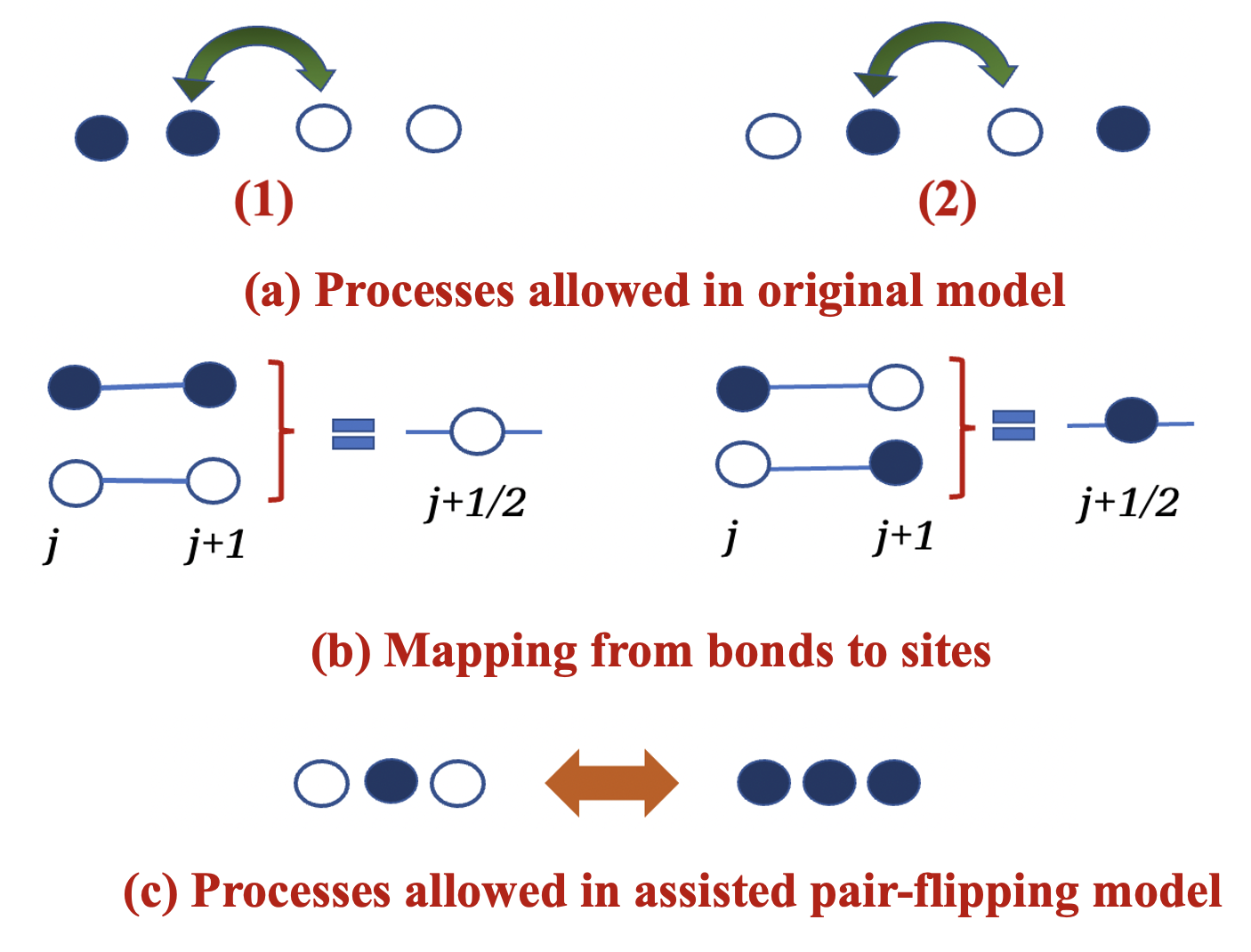
Figure 1: (a) Processes allowed in original correlated-hopping model with terms involving four consecutive sites. (b) Mapping of bonds to sites. (c) The bond-site mapping converts the correlated-hopping model to an assisted pair-flipping model with terms involving three consecutive sites. Here filled and empty circles represent occupied and unoccupied sites respectively.

III Fragmentation of the Hilbert space

In this section, we will show how kinetic constraints in this model shatters the Hilbert space leading to an exponentially large number of fragments in the local number basis. The fragmentation structure can appear in a variety of forms, such as frozen fragments consisting of a single eigenstate of the Hamiltonian and finite-dimensional fragments within a symmetry-resolved fragment of the total Hilbert space.

III.1 Irreducible strings

We first discuss the fragmentation structure in three-site model which allows the transition described in Eq. (5); the analytical treatment is much simpler in the three-site language. It is convenient to define a Hamiltonian which only has matrix elements between the states $010$ and $111$. We therefore define Pauli matrices $\sigma_{j}^{\alpha}$ at site $j$ (where $\alpha=x,y,z$), so that states 1 and 0 at site j corresponds to $\sigma_{j}^{z}=\pm 1$. In terms of these Pauli spin operators, the Hamiltonian becomes

$$H_{3}=\sum_{j}~{}(\sigma_{j-1}^{+}\sigma_{j+1}^{+}+\sigma_{j-1}^{-}\sigma_{j+1}^{-})\,\left(\frac{1+\sigma_{j}^{z}}{2}\right).$$ (7)

Note that this expression differs from $H_{2}$ in that it is defined in terms of Pauli spin operators which commute at different sites. This is an assisted spin-flipping Hamiltonian in which a pair of spins can flip on next-nearest-neighbor sites provided the site in the middle has spin $\uparrow$. The number of states in a system with $L$ sites is $2^{L}$. We will consider open boundary conditions (OBC) to perform our analysis of fragmentation. One should note that the transition rules shown in Eq. (7) imply that

$$11110\leftrightarrow 01010\leftrightarrow 01111.$$ (8)

This implies that a string of four 1’s can move across either a 0 or a 1 (trivially). This will be important later to understand different features of the HSF occurring in this model.

We will show in this paper that the model in Eq. (7) has an exponentially large number of fragments. These fragments are most easily characterized in terms of a construction called the IS which act as an exponentially large number of conserved quantities. This construction of IS is a variation of the construction used earlier  Menon and Dhar (1995); Menon et al. (1997); Barma and Dhar (1994a). This is defined as follows.

A basis configuration is characterized by a binary string of length $L$, e.g., $0011010\cdots$. We read the string from left to right, move the first occurrence of $1111$ to the left end of the string and then delete it. This reduces the length of the string by $4$. We repeat this till no further reduction is possible. Then, we read the current string from left to right, and change the first occurrence of $010$ to $111$. If this generates a $1111$, we delete this to get a string of reduced length. The steps $1111\rightarrow\phi$ (null string), and $010\rightarrow 111$ are repeated, till no further change can be made. The final string is the IS corresponding to the initial string. As an example, one can easily see that the IS for a binary string configuration $01111010101$ reduces to $001$ due the rules mentioned earlier, as also depicted in Fig. 2.

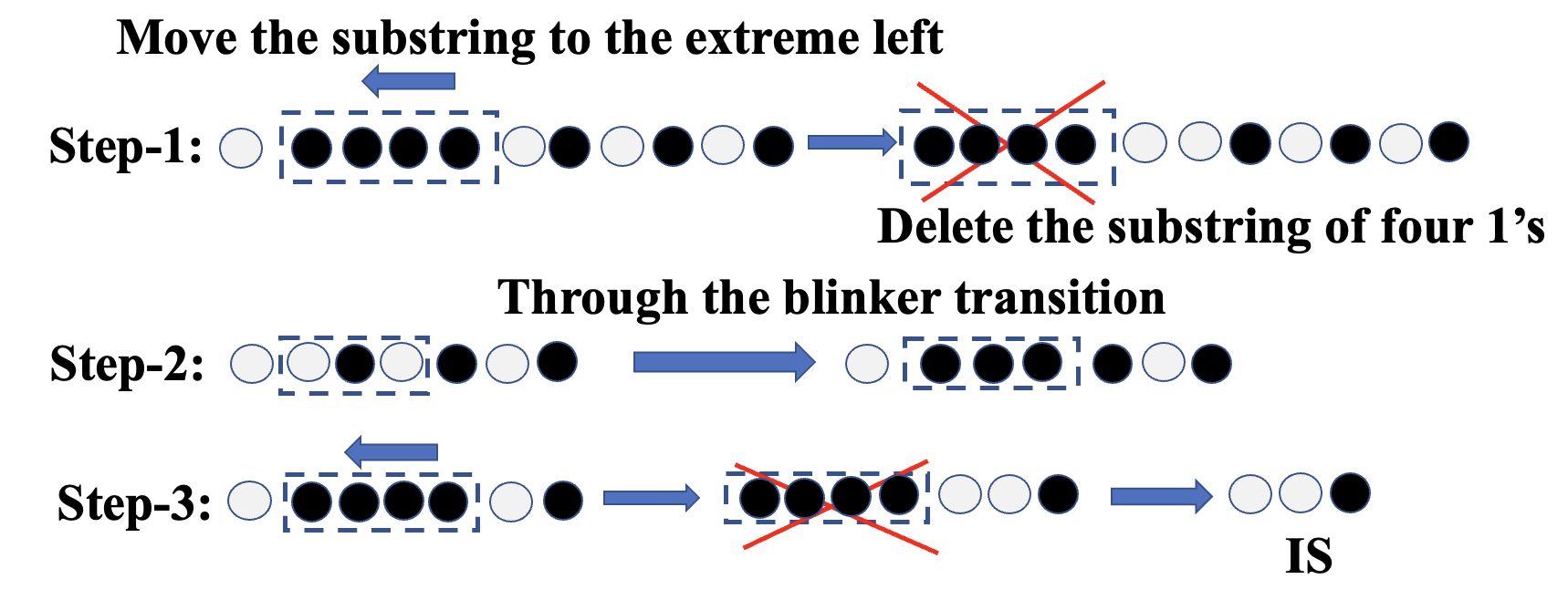
Figure 2: Illustration of IS construction for a given binary string configuration.

The usefulness of the IS construction comes from the observation that any states belong to the same fragment if and only if they have the same IS. To prove this assertion, we note that the strings $01111$ and $11110$ are obtainable from each other as shown in Eq. (8). Hence one may treat a group of four adjacent $1$’s as a block that can slide across a $0$, and it can slide across a $1$ trivially. Thus, we can push any such blocks of $1111$ to the left end of the system and delete them.

An IS of length $L-4r$ corresponds to a root state of length $L$ which has $4r$ $1$’s at the left. We also note that for each of the steps going from the initial string to the root state, the inverse steps are also allowed through the transitions $010\leftrightarrow 111$. So, if two configurations have the same root state, they can be reached from each other. The Hilbert space fragment corresponding to a given IS is spanned by all the configurations that have this IS. Thus the IS acts as a unique label for the fragment.

III.2 Determining the number of fragments

To calculate the number of fragments, it is convenient to define a number $M(n)$ which is the number of distinct IS of length $n$. We know that a IS cannot contain the substrings $010$ or $1111$ anywhere. Using this fact, we can calculate $M(n)$, for $n>3$, using a transfer matrix method as shown in Appendix A.

$n$	0	1	2	3	4	5	6	7	8	9	10	11	12
$M(n)$	1	2	4	7	11	18	29	47	76	123	199	322	521

Table 1: Values of $M(n)$ versus $n$.

It is convenient to define $M(0)=1$. Clearly, $M(1)=2$, $M(2)=4$ and $M(3)=7$. The results for the first few values of $M$ are given in Table I. Given $M(n)$, the number of fragments of length $L$ with OBC is given by

$$N_{OBC}(L)~{}=~{}\sum_{r=0}^{\lfloor L/4\rfloor}M(L-4r),{\rm~{}for~{}}L>4.$$

(9)

The resulting values are used to analytically calculate the $N_{OBC}(L)$, given in Table II; we have verified these values numerically. We also list the corresponding values for PBC found numerically (using a method described in Appendix A). We find that both $N_{OBC}$ and $N_{PBC}$ grow asymptotically as $\tau^{L}$, where $\tau=(\sqrt{5}+1)/2\simeq 1.618$ is the golden ratio.

$L$	4	5	6	7	8	9	10	11	12
$N_{\rm OBC}$	12	20	33	54	88	143	232	376	609
$N_{\rm PBC}$	10	13	20	32	59	81	131	207	363

Table 2: Values of $N_{OBC}$ and $N_{PBC}$ versus $L$ obtained by numerical enumeration.

In Fig. 3 we show the distribution of fragment numbers for different system sizes with OBC. Fragment size equal to 1 (left edge of the figure) corresponds to frozen fragments which are discussed in Sec. III.3. The largest fragment (right edge of the figure) will be discussed in Sec. III.5.

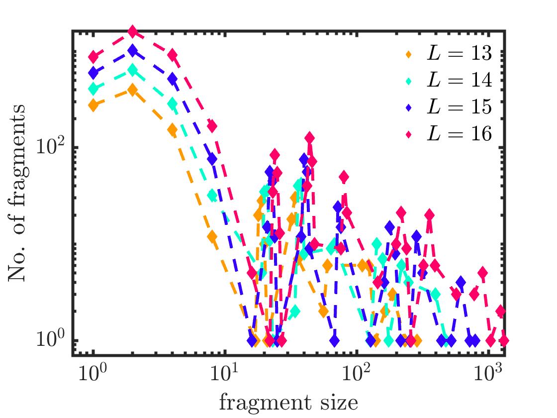
Figure 3: Plot showing the distribution of number of fragments versus dimensions of fragments for four different system sizes, $L=13,14,15$ and $16$, with OBC.

III.3 Description of frozen fragments

The model contains an exponentially large number of eigenstates that do not participate in the dynamics; we call these “frozen” states. The frozen states $|f_{j}\rangle$ are all product states in the particle number basis, and are annihilated by the Hamiltonian such that $H|f_{j}\rangle=0$. Hence these states are zero-energy eigenstates of the model Hamiltonian. Two trivial examples of such states in terms of the four-site language are fully empty and fully occupied states in the particle number basis, i.e., $|\cdots 0000\cdots\rangle$ and $|\cdots 1111\cdots\rangle$, respectively.

In a frozen state, there cannot be any occurrence of substrings $010$ or $111$, and the length of the IS must be $L$. It is then straightforward to set up a transfer matrix to determine the exact numbers of such states $N^{frozen}(L)$ for a system of size $L$. The details of the calculation are given in Appendix B. We find that the number of frozen fragments for a system of size $L$ grows as $1.466^{L}$ for large $L$. For the first few values of $L$, the number of frozen states $N^{frozen}(L)$ is shown in Table III for both OBC and PBC.

$L$	3	4	5	6	7	8	9	10	11	12
$N^{frozen}_{\rm OBC}$	6	9	13	19	28	41	60	88	129	189
$N^{frozen}_{\rm PBC}$	4	5	6	10	15	21	31	46	67	98

Table 3: $N^{frozen}_{\rm OBC}$ and $N^{frozen}_{\rm PBC}$ versus $L$ with OBC and PBC respectively.

III.4 Description of some simple integrable fragments

We will now present some examples of fragments which consist of more than one state (and are therefore not frozen) but in which the Hamiltonian dynamics is integrable.

The first example of an integrable fragment is a set of multiple ”blinkers” each of which flips back and forth between two states. For example, we can have an IS of the form

$$\cdots 00011100111000\cdots$$

These fragments consist of a sea of $0$’s with islands of three consecutive sites that can flip between $010$ and $111$ but are fully localized in space. The general state in such a fragment can be obtained by concatenating the substrings $0$, $1110$ and $0100$. For a system with OBC, the number of states in the fragment can be found by defining a transfer matrix $T$ following a procedure similar to the one given in Appendix A. We find that $T$ is a $8\times 8$ matrix whose characteristic polynomial is given by $\lambda^{5}(\lambda^{3}-\lambda^{2}-1)$. The largest root of this equation is approximately $1.466$ (see Eqs. (36) and (37)), and the number of states therefore grows with system size as $1.466^{L}$. For each blinker, labeled by an integer $j=1,2,\cdots,r$, we can introduce a Pauli matrix $\tau_{j}^{z}$ which is equal to $\pm 1$ for $111$ and $010$ respectively. The number of states in this fragment is equal to $2^{r}$, and the effective Hamiltonian is given by $H_{eff}=\sum_{j=1}^{r}\tau_{j}^{x}$. It is then easily seen that the energy eigenvalues for this fragment are given by $\sum_{j=1}^{r}e_{j}$, where each $e_{j}$ can take values $\pm 1$.

The second example we consider is a fragment whose IS is made of $L-4$ $0$’s. The configuration will have a single substring $1111$ or a single substring $101$ in a sea of zeroes; the total number of such states is $2L-5$. We can think of these as the states of a particle which can be either in a state $a_{j+3/2}=1111$ at sites $(j,j+1,j+2,j+3)$, where $j=1,2,\cdots,L-3$, or in a state $b_{j}=101$ at sites $(j-1,j,j+1)$, where $j=2,L-1$. The Hamiltonian can take the state $|a_{j+3/2}\rangle$ to either $|b_{j+1}\rangle$ or $|b_{j+2}\rangle$. This gives us a tight-binding model of a particle that moves on a finite line with $2L-5$ sites. We then find that the energy levels of this effective Hamiltonian are

$$E_{k}=2\cos[\pi k/(2L-4)],{\rm~{}where~{}}k=1,\cdots,2L-5.$$ (10)

III.5 Description of the largest fragment

We now consider the largest fragment, which includes all the states reachable from the configuration of all $1$’s. The corresponding IS reduces to one of the four possibilities $\phi$ (null string) or $1$ or $11$ or $111$. Let $D_{L}$ denote the dimension of the fragment corresponding to the IS given by $111\cdots 111$, i.e., 1 repeated $L$ times. We will compute the generating function

$$V(x)~{}=~{}\sum_{L=0}^{\infty}~{}D_{L}~{}x^{L}.$$ (11)

Following a lengthy calculation whose details are shown in Appendix C, we obtain the expression

$$V(x)=\frac{1}{1~{}-~{}x~{}-~{}\left(\frac{1~{}-~{}\sqrt{1-12x^{4}}}{6x}\right)}.$$ (12)

Writing this in the form given in Eq. (11), we find that the growth of $D_{L}$ for large $L$ is determined by the singularities of $V(x)$ lying closest to the origin Menon and Dhar (1995); Menon et al. (1997); Barma and Dhar (1994a). According to Eq. (12), these singularities lie at $x_{0}^{4}=1/12$, namely, the fourth roots of $1/12$. Hence $D_{L}$ grows as $(1/|x_{0}|)^{L}$, i.e., $1.8612^{L}$ for large $L$. To confirm this, we Taylor expand Eq. (12) which generates the series

$$V(x) = 1+x+x^{2}+2x^{3}+3x^{4}+4x^{5}+6x^{6}+12x^{7}+19x^{8}+28x^{9}+46x^{10}+92x^{11}+150x^{12}+232x^{13}+396x^{14}$$

$$+792x^{15}+1315x^{16}+2092x^{17}+3646x^{18}+7292x^{19}+12258x^{20}+19864x^{21}+35076x^{22}+70152x^{23}+\cdots,$$

We have checked that these numbers perfectly agree with those obtained by brute force numerical enumeration. We note that the exponential growth rate of the largest sector with $L$ is slower than the total number of states $2^{L}$, and goes to zero in the limit of large $L$, which establishes the strong fragmentation Sala et al. (2020) of the Hilbert space in this model.

IV Subspace restricted ETH in systems with strong Hilbert space fragmentation

The existence of frozen states and integrable fragments (such as fragments with $n$ blinkers) implies that strong ETH is not satisfied with respect to the full Hilbert space in our model. In earlier discussions of weak ETH, these are usually treated as thermodynamically unimportant exceptions since these states have only a small probability of being realized.

To take all these small fragments into account, one can modify the ETH as follows. Suppose that a Hamiltonian in a basis given by products of local states has a block structure, such that eigenvectors of energy have non-zero components only within a single block. Then it seems natural to postulate that reduced density matrices calculated from the eigenvectors of a local observable will tend to values corresponding to a restricted microcanonical ensemble, in which all the eigenvectors within a block having a given energy density are equally likely. We shall call this the subspace restricted ETH. We can see that this is satisfied even for fragments with only one state (i.e., frozen fragments), and for fragments with only blinkers.

We will now check the validity of ETH in other sectors in the full Hilbert space at half-filling, as well as the validity of a weaker version of ETH within the largest fragment. We first examine the variation of expectation values of local observables for all eigenstates of the Hamiltonian and the variation of the half-chain entanglement entropy $S_{L/2}$ as a function of the energy $E$ without resolving the fragmentation structure. In Figs. 4 (a) and (b), we show the expectation values of the local observables $\langle n_{L/2}\rangle$ and $\langle n_{L/2+1}n_{L/2}\rangle$ as a function of the energy density $E/L$ for all the eigenstates for three different system sizes, $L=12,14$ and $16$. We see that the widths of the distributions do not decrease significantly with increasing system sizes. Moreover, we also analyze the standard deviations of the differences of $\langle E|A|E\rangle-\langle A\rangle_{E}$, where $|E\rangle$ denotes an eigenstate of the Hamiltonian at energy $E$, and $\langle A\rangle_{E}$ is the microcanonical expectation value of $A$ at energy $E$ obtained by averaging over eigenstates within an energy window $\Delta E/L=0.025$ Beugeling et al. (2014). For our case, we consider $A$ to be $n_{L/2}$ and $n_{L/2+1}n_{L/2}$, and then examine the standard deviation $\sigma_{A}$ as a function of the total Hilbert space dimension $D$ at half-filling, as shown in Figs. 4 (c) and (d). In both cases, we observe that the values of $\sigma_{A}$ do not change notably with increasing values of $D$. This confirms that the strong version of diagonal ETH is not valid in our model within the full Hilbert space at half-filling. Similar behavior was seen earlier in other models showing HSF  Srednicki (1994); Deutsch (1991).

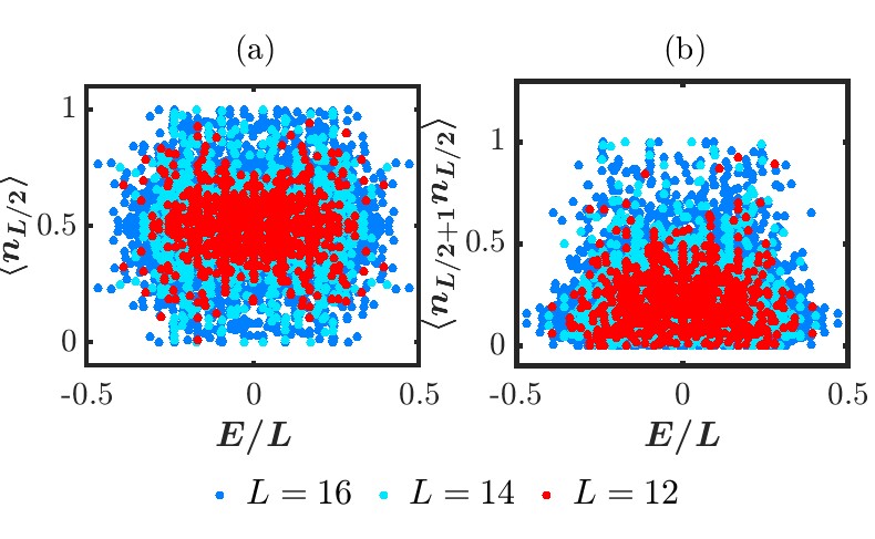
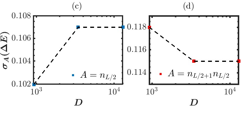
Figure 4: Scatter plots of (a) $\langle n_{L/2}\rangle$ and (b) $\langle n_{L/2+1}n_{L/2}\rangle$ for all the eigenstates as a function of energy density $E/L$ for different system sizes, $L=12,14$ and $16$. In all three cases, the widths of the distribution do not appear to decrease significantly with increasing $L$. The standard deviation $\sigma_{A}$ of $\langle n_{L/2}\rangle$ and $\langle n_{L/2+1}n_{L/2}\rangle$ as a function of Hilbert space dimension $D$ in an energy window of $\Delta E/L~{}=~{}0.025$ are shown in plots (c) and (d). The values of $\sigma_{A}$ do not decrease significantly with increasing Hilbert space dimensions similar to Figs. (a-b); this behavior is also not consistent with strong ETH.

Next, we discuss the spectrum of the half-chain entanglement entropy $S_{L/2}$ as a function of the energy $E$ for the full Hilbert space (without resolving the individual fragment) at half-filling with OBC for three different system sizes, $L=14,16$ and $18$. This is shown in Figs. 5 (a-c). In all three figures, we see that many low-entanglement states are present in the middle of the spectrum. Further, the values of entanglement entropies for all the eigenstates are much smaller than the thermal value $S_{page}=(L\ln 2-1)/2$ Page (1993) shown by the dash-dot lines; this again shows that ETH with respect to the full Hilbert space is not satisfied. Moreover, the entropies of the eigenstates do not fall on a particular line when plotted against the energy. Rather they are distributed over values which are much smaller than the thermal value, which is exactly the opposite of what is typically observed for a system obeying strong ETH. Also, the width of the entanglement entropy spectrum does not shrink with increasing $L$ unlike a thermal system, indicating a manifestly non-thermalizing behavior as a consequence of strong HSF.

Next, we study the energy level spacing distribution which is often studied to probe whether a model is integrable or non-integrable Wigner (1955); Serbyn et al. (2016); Pal and Huse (2010). It is well-known from the theory of random matrices that non-integrable systems described by random matrices show level repulsion, but integrable models, or models with extra conserved quantities do not. To quantify the degree of level repulsion in a model, it is often better to study the level spacing ratios rather than the level spacing distribution of the sorted eigenspectrum. To do so, we define the level spacing ratios of the sorted eigenspectrum by $r_{n}=\delta_{n+1}/\delta_{n}$, where $\delta_{n}=E_{n+1}-E_{n}$ and $E_{n}$ is the $n$-th energy eigenvalue. If a system is integrable, $r$ follows the Poisson distribution, i.e., $P(r)=1/(1+r)^{2}$, while non-integrable systems described by real Hermitian Hamiltonians follow the Gaussian orthogonal ensemble (GOE) distribution Atas et al. (2013); Berry and Tabor (1977) which is given by the distribution

$$P(r)~{}=~{}\frac{27}{8}\frac{(r+r^{2})}{(1+r+r^{2})^{5/2}}.$$ (14)

It is also convenient to study the distribution of $\tilde{r}$, which is defined as

$$\tilde{r}_{n}~{}=~{}\frac{\text{min}(\delta_{n+1},\delta_{n})}{\text{max}(\delta_{n+1},\delta_{n})}~{}=~{}\text{min}(r_{n},1/r_{n}).$$ (15)

For the two classes mentioned above, the distribution of $\tilde{r}$ follows $P(\tilde{r})=2P(r)\,\theta(1-r)$, where $\langle\tilde{r}\rangle=0.386$ for Poisson and $0.536$ for GOE.

To numerically compute the level spacing statistics of the consecutive energy levels for the sorted eigenspectrum of the full system, we add a small uniformly distributed random on-site potential with strength $w=0.01$ for an $18$-site system of $L=18$ with OBC to break all the discrete symmetries and to eliminate any accidental degeneracies  Moudgalya and Motrunich (2022); Moudgalya et al. (2020); Herviou et al. (2021). We note that the presence of an on-site disorder preserves the fragmentation structure of the full Hilbert space. In addition, we also impose the half-filling condition with to choose a particular $C_{1}$ symmetry sector, but we do not restrict the analysis within particular $C_{2}$ and $C_{3}$ symmetry fragments since these two global symmetries are only well-defined for $L=4n$. As shown in Fig. 5 (d), we see that the distribution of $\tilde{r}$, called $P(\tilde{r})$, is indistinguishable from a Poisson curve with $\langle\tilde{r}\rangle\simeq 0.383$; this is very close to the value observed for an integrable system. The exponentially large number of dynamically disconnected fragments act as large number of conserved quantum numbers that forbid level repulsion as in an integrable system Herviou et al. (2021); Kwan et al. (2023).

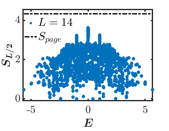
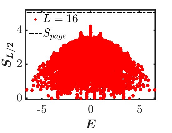
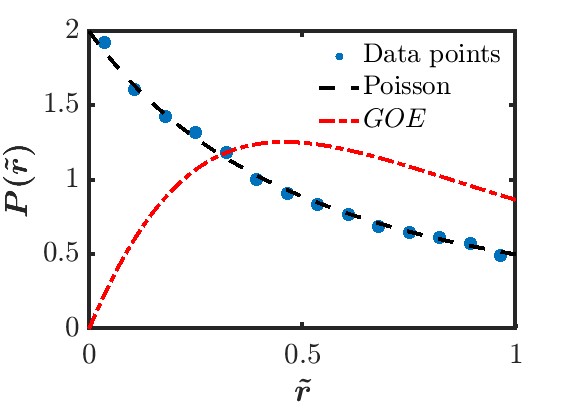
(a)(b)
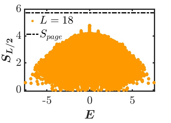
(c)(d)

Figure 5: (a-c) Plots showing the half-chain entanglement entropy, $S_{L/2}$ versus $E$ for the full Hilbert space at half-filling for $L=14$, $16$ and $18$, respectively, with OBC. In all three cases, the entanglement entropies of all the eigenstates do not fall on a line, and they have values much smaller than the thermal value. Also, the widths of the spectra do not decrease with increasing $L$, indicating that strong ETH is not valid. (d) Plot showing the probability distribution of $\tilde{r}$ for the sorted eigenspectrum for the full Hilbert space at half-filling for a $18$-site system with OBC. (In order to break any discrete symmetries, we add a small uniformly distributed random on-site potential with strength $w=0.01$. The disorder preserves the fragment structure of the full Hilbert space). The distribution $P(\tilde{r})$ follows a Poison curve with $\langle r\rangle\simeq 0.383$.

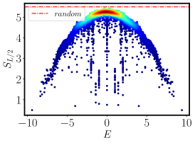
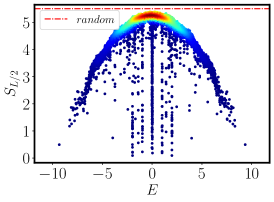
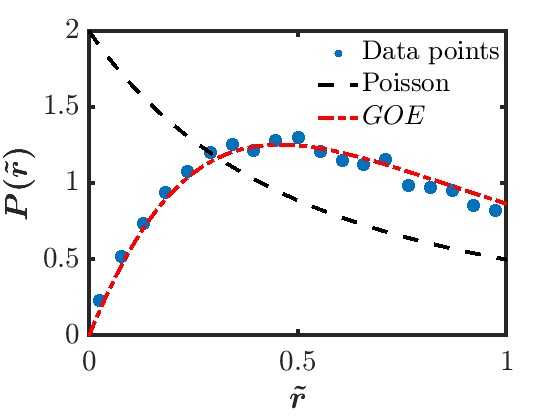
(a) (b)(c)

Figure 6: (a-b) Plots showing the half-chain entanglement entropy $S_{L/2}$ versus $E$ for the largest fragment produced by enumerating the root configuration $1010\cdots 1010$ in the four-site model for $L=22$ (the fragment size is $19864$) with OBC with (a) no disorder and (b) a small uniformly distributed disorder with strength $w=0.01$, respectively. (a) The entropies for most of the eigenstates within this fragment fall on a line, apart from some low-entanglement outlying eigenstates in the middle of the spectrum. (b) The spectrum in the presence of disorder exhibits identical features. In both cases, the red dash-dot line denotes the entanglement entropy of a random state within this particular fragment. (c) Plot of the probability distribution $P(\tilde{r})$ versus $\tilde{r}$ for case (b). $P(\tilde{r})$ obeys the GOE distribution, indicating non-integrability of this fragment.

Finally, we study the behavior of the largest fragment generated by enumerating the root state $1010\cdots 1010$ for the original model with terms involving four consecutive sites for $L=22$ with OBC (the size of this fragment is $19864$). In the three-site model, this state reduces to the state $111\cdots 111$, which generates the largest fragment. In Fig. 6 (a), we show the entanglement entropy as a function of $E$ for the largest fragment. We see that the entropies of most of the eigenstates fall on a curve, with a small number of outlying low-entanglement eigenstates in the middle of the spectrum. In Fig. 6 (b), we perform the same analysis with a small uniformly distributed random on-site disorder with strength $w=0.01$ to discard any discrete symmetries and to avoid any accidental degeneracies Moudgalya and Motrunich (2022); Moudgalya et al. (2020). (The random on-site disorder preserves the fragment structure). We see that the spectrum in this case shows features identical to the previous case; further, it stabilizes the low-entanglement eigenstates, as can be seen in Fig. 6 (b). We find that the consecutive energy level spacing statistics for the eigenstates within this fragment with small disorder is consistent with GOE level statistics with $\langle\tilde{r}\rangle\simeq 0.524$ which is close to the GOE value. This points towards non-integrability of the largest fragment Moudgalya et al. (2020), as shown in Fig. 6 (c).

In Figs. 7 (a) and (b), we show the average values of $n_{L/2}$ and $n_{L/2+1}n_{L/2}$ for all the eigenstates within this subspace for $L=14,16,18$ and $20$ where the fragment sizes are $232,~{}792,~{}2092$ and $7292$, respectively. We see that the width of this distribution becomes narrower with increasing system size. We then perform the same analysis as Figs. 4 (c) and (d) within the largest fragment in Figs. 7 (c-d). We see that the standard deviations $\sigma_{A}$ of local observables decrease with increasing values of fragment size $D$. Moreover, $\sigma_{A}$ approximately scales as $~{}1/\sqrt{D}$ with some deviation, which has been seen earlier in the ETH obeying systems Beugeling et al. (2014). This behavior again indicates that the subspace-restricted diagonal ETH is satisfied within this fragment. However, there are some outlying states which do not show thermal behavior as shown in 7 (a) and (b).

Despite the fact that ETH is not valid with respect to the full Hilbert space as shown in Figs. 4 and 5, expectation values of local observables of eigenstates within sufficiently large fragments still satisfy ETH as shown in Figs. 6 and 7. Therefore, sufficiently large fragments still satisfy ETH even in the case of strongly fragmented systems. This is also dubbed as Krylov-restricted thermalization in the literature Moudgalya et al. (2020, 2022); Stephen et al. (2024). This kind of restricted thermalization has a significant impact on the dynamics of the system, in particular, atypical dynamical behavior of correlation functions, which we will discuss in the next section.

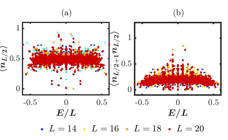
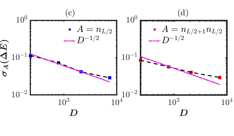
Figure 7: Plots of (a) $\langle n_{L/2}\rangle$ and (b) $\langle n_{L/2+1}n_{L/2}\rangle$ for all the eigenstates within the largest fragment of the full Hilbert space. Most of the eigenstates within this fragment show a thermal behavior. In both cases, the bulk of the distribution becomes narrower with increasing $L$, but with some outlying states which do not fit within a narrow window of values of $\langle n_{L/2}\rangle$ and $\langle n_{L/2+1}n_{L/2}\rangle$. The standard deviations $\sigma_{A}$ of $\langle n_{L/2}\rangle$ and $\langle n_{L/2+1}n_{L/2}\rangle$ as a function of the size $D$ of the largest fragment within an energy window of $\Delta E/L~{}=~{}0.025$ are shown in plots (c) and (d). We see that the values of $\sigma_{A}$ decrease with increasing sizes of largest fragment, which approximately scale as $1/\sqrt{D}$ with a slight deviation. The decreasing values of $\sigma_{A}$ with increasing fragment size supports the subspace-restricted ETH within the largest fragment.

V Dynamical signatures of Hilbert space fragmentation

In this section, we will study various autocorrelation functions as dynamical signatures of the absence of thermalization due to HSF.

V.1 Long-time behavior of autocorrelation functions

As a signature of the lack of thermalization due to strong HSF, we first investigate the behavior of the time-dependent correlation function

$$C_{j}(t)=\langle\psi|(n_{j}(t)-1/2)(n_{j}(0)-1/2)|\psi\rangle,$$

where $n_{j}$ is the fermion number operator at site $j$, $|\psi\rangle$ being a typical random initial state in the full Hilbert space, which is chosen to have the form $|\psi\rangle=\sum_{j}a_{j}|f_{j}\rangle$ with $\sum_{j}|a_{j}|^{2}=1$, where the $a_{j}$’s are random numbers and $|f_{j}\rangle$ denote Fock space basis states. We will take the density to be $1/2$ and open boundary conditions.

In thermal equilibrium, the autocorrelation function is expected to decay to zero as $1/L$ for a system of length $L$. In Fig. 8 (a), we study the boundary autocorrelator, $C_{1}(t)$ for a system size $L=18$ with OBC at half-filling for a random initial state on the Hilbert space. We find persistent oscillations around a finite saturation value of about $0.115$ (shown in the inset of the plot) up to a long time $t\sim 10^{3}$. We then study the same function in the middle of the system, $C_{L/2}(t)$, for the same system size in Fig. 8 (b). We observe that $C_{L/2}(t)$ saturates to a much smaller value of about $0.045$ (shown inset of the plot) at long times. In a similar manner, we show the same quantities for $L=20$ in Fig. 8 (c-d). We see that the behaviors of $C_{1}(t)$ and $C_{L/2}(t)$, including the period of oscillations, do not significantly change with increasing system size. However, both quantities oscillate around finite saturation values given by $0.113$ and $0.04$, respectively (shown in the insets of the plots), which are slightly smaller compared to Figs. 8 (a) - 8 (b), respectively. We therefore conclude that the boundary correlator behaves in a different manner from the bulk correlator.

Further, strong HSF leads to an non-uniform profile of correlation function near the edge of the chain in our model model as was observed earlier in this context for other models Sala et al. (2020); Rakovszky et al. (2020); Moudgalya and Motrunich (2022). We examine the robustness of this non-uniform profile near the edge against perturbations by including two types of terms in the four-site Hamiltonian. The first one is a uniformly distributed random on-site potential of strength $w=0.1$, and the results are shown in Figs. 9 (a) and 9 (c). The second one involves the Hamiltonian

$$H^{\prime}~{}=~{}\sum_{j}\left[(n_{j-1}-n_{j+2})^{2}~{}-~{}\epsilon\right](c_{j}^{\dagger}c_{j+1}+c_{j+1}^{\dagger}c_{j})$$ (16)

where $\epsilon=0.1$, giving the results shown in Figs. 9 (b) and 9 (d). The first one breaks all the discrete symmetries present in the four-site model, but it preserves the fragmentation structure of the full Hilbert space. On the other hand, the second one preserves all the discrete symmetries but modifies the fragmentation structure of the full Hilbert space; the numbers of fragments generally decreases for this case since the $\epsilon$ terms connects certain states which are not connected otherwise. As shown in Figs. 9 (a) and 9 (c), the long-time behaviors of $C_{1}$ and $C_{L/2}$ in the first case remains the same as in the unperturbed case, exhibiting an absence of thermalization. For the second case, both the correlators decay to zero after showing a non-trivial intermediate-time dynamics, as can be seen in Figs. 9 (b) and Fig. 9 (d).

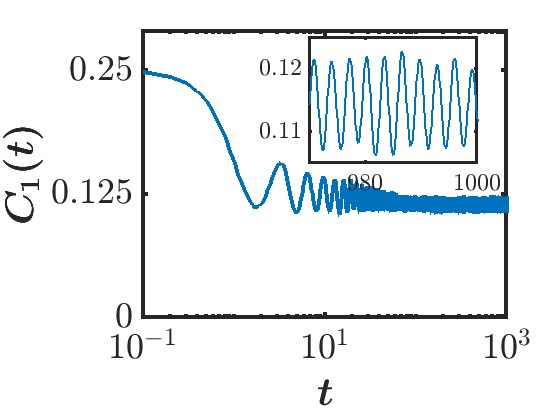
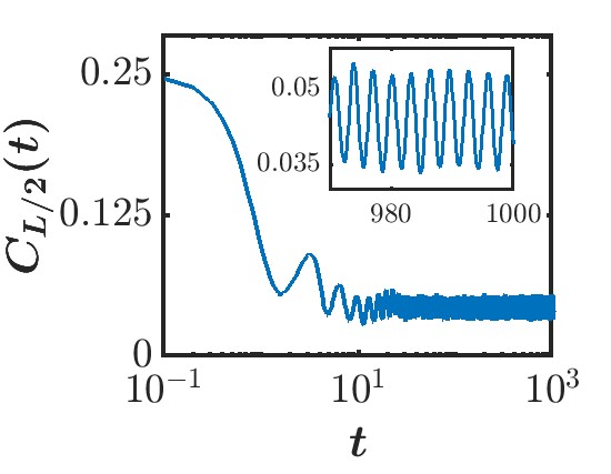
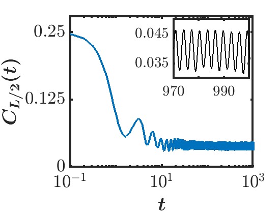
(a) (b)
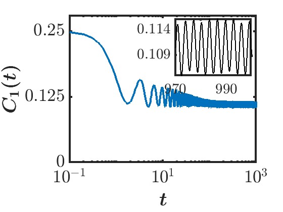
(c) (d)

Figure 8: (a-b) Plots showing the long-time behaviors of the boundary and bulk correlators, $C_{1}(t)$ and $C_{L/2}(t)$, respectively, starting from a typical random initial state at half-filling with OBC for $L=18$. (c-d) Similar plots for $L=20$. (a) $C_{1}(t)$ oscillates around a finite saturation value of about $0.115$ at long times, revealing non-thermal behavior near the boundary of the system. (b) $C_{L/2}(t)$ oscillates around a finite saturation value of about $0.045$, which is much smaller than the boundary case. (c) $C_{1}(t)$ for this case oscillates around a finite saturation of about $0.113$ at long times, which is slightly smaller compared to that observed in Fig. (a). (d) In this case, $C_{L/2}$ again shows similar behavior as Fig. (b), but it oscillates around a saturation value ($\sim 0.04$), again slightly smaller compared to Fig. (b). In all four cases, the last ten oscillations for $970\leq t\leq 1000$ are shown in the insets of the plots.

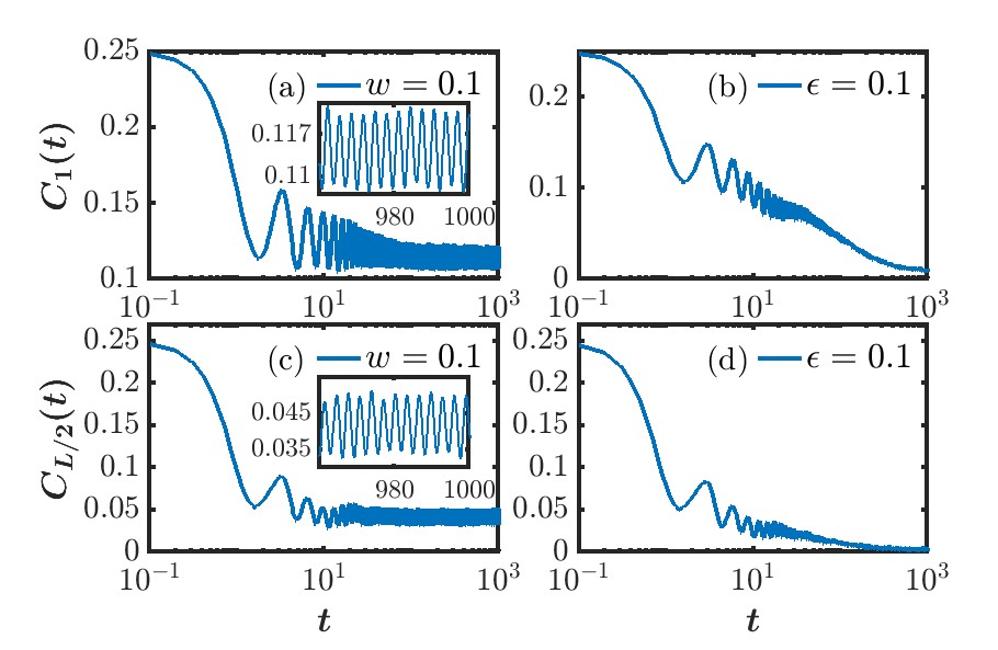
Figure 9: (a-b) Plots showing the long-time behavior of the boundary correlator $C_{1}(t)$ starting from a typical random initial state for $L=18$ at half-filling with OBC in the presence of two kinds of perturbations, uniformly distributed random disorder with disorder strength $w=0.1$, and the perturbation term with $\epsilon=0.1$ shown in Eq. (16). (a) $C_{1}(t)$ oscillates around a finite value of about $0.12$ in the long-time limit just as in the unperturbed case. (b) $C_{1}(t)$ decays to zero at long times after exhibiting a non-trivial intermediate-time dynamics close to the saturation value of the unperturbed model. (c-d) Plots showing the long-time behaviors of bulk correlators, $C_{L/2}(t)$ starting from a random initial state again for the same two cases. (c) $C_{L/2}(t)$ in the presence of random disorder again shows a behavior similar to the unperturbed case. (d) $C_{L/2}(t)$ for this case decays to zero at long times, after exhibiting non-trivial intermediate-time dynamics like the boundary case. In Figs. (a) and (c), the last ten oscillations for $970\leq t\leq 1000$ are shown in the insets of the plots.

We will now explain the long-time saturation value of the autocorrelation functions by taking the fragmentation structure of the full Hilbert space into account. It can be shown that the equilibrium value of $C_{j}(t)$ predicted by the ETH hypothesis is zero for all values of $j$ if our model thermalizes. Therefore, the nonuniform profile of autocorrelation function near the edge of the chain shown in Fig. 8 is an atypical behavior as a consequence of subspace-restricted ETH due to strong HSF. This behavior can be explained with the help of the Mazur inequality Mazur (1969), which applies to the long-time averages of autocorrelation functions in the context of thermalization. For quantum systems, an exact Mazur-type equality was obtained by Suzuki Suzuki (1971), which takes into account existence of constants of motion in the problem. In the same spirit, the value of the Mazur bound for fragmented Hilbert spaces is changed by taking into account the structures of invariant subspaces. We do this as follows.

We define $P_{i}$ as the projection operator onto a particular fragment $\mathcal{H}_{i}$ with dimension $\mathcal{D}_{i}$. The set of projectors onto different fragments form a complete orthogonal set of conserved quantities such that $P_{i}P_{j}=\delta_{ij}P_{j}$. Using these, we define the long-time averaged autocorrelation functions

$$F_{j}= \lim_{T\rightarrow 0}\,\frac{1}{T}~{}\int_{0}^{T}\,dt\,\langle(n_{j}(t)-\frac{1}{2})(n_{j}(0)-\frac{1}{2})\rangle,$$

where $n_{j}$ is the fermion number operator at site $j$. These satisfy the inequality due to Mazur Mazur (1969)

$$F_{j}\geq~{}\sum_{i}~{}\frac{\left({\rm Tr}[P_{i}(n_{j}-\frac{1}{2})P_{i}]\right)^{2}}{DD_{i}}~{}\equiv~{}C_{j}(\infty),$$ (17)

Here $D_{i}$ is the dimensionality of the $i$-th fragment, and $D$ is the toal Hilbert space dimension (here $D=2^{N}$).

In Fig. 10 (a), we plot the variation of the infinite-time saturation value of boundary and bulk autocorrelation functions, $C_{1}^{M}(\infty)$ and $C_{L/2}^{M}(\infty)$, obtained using Eq. (17) for an $L-$site system with OBC. We find that the Mazur bound in the bulk of the chain decays as $1/L$ for comparatively large system sizes like the assisted pair-flipping model. On the other hand, the Mazur bound at the boundary of the chain saturates to approximately $0.12$. We show the Mazur bound as a function of the site index for different system sizes in Fig. 10 (b); this shows a non-uniform profile, being smaller at the centre compared to the ends. Further, HSF leads to localization close to the edge of the chain which has been dubbed as “statistical edge localization” Rakovszky et al. (2020); Moudgalya et al. (2022); we see this in the long-time behavior of boundary autocorrelation functions shown in Figs. 8 (a) and (b). We note here that the late-time average of the bulk autocorrelator decaying with system size as $1/L$ usually indicates thermal behavior of the bulk states. On the other hand, the localized profile of the autocorrelator near the edge shows non-thermal nature of the boundary spectrum. This implies that the non-local conserved quantities arising due to HSF do not have any significant impact on the thermal behavior of the bulk states for our model, in contrast to the boundary states. However, this numerical observation requires a more careful investigation since our analysis has only been carried out for rather small system sizes. In some cases, it has been observed that such thermal behavior of the bulk autocorrelators is an artifact of limited system sizes, and the decay can deviate significantly from $1/L$ in the thermodynamic limit. Specifically, the decay can go as $1/L^{a}$ where $a<1$ Hart (2023).

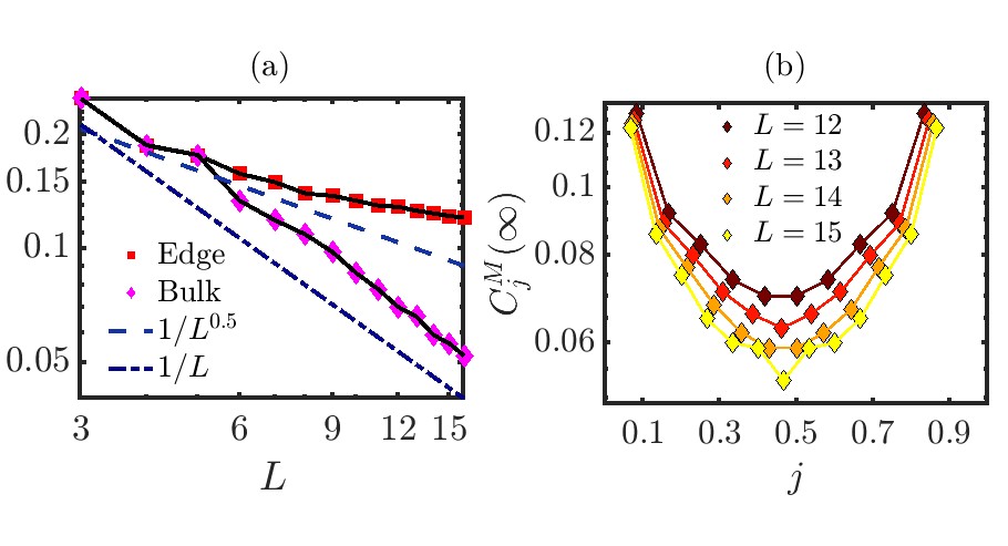
Figure 10: (a) Log-log plot showing the lower bounds of the infinite-time boundary and bulk correlators predicted by the Mazur inequality for different system sizes. In the bulk of the chain, the Mazur bound follows a $1/L$ curve instead of $1/\sqrt{L}$ (as depicted by two guiding lines), while near the edge of the chain, the Mazur bound shows a localized behavior and saturates to approximately $0.12$. (b) The variation of the Mazur bound across the chain for different sizes exhibits a non-uniform profile due to the strong HSF in our model.

V.2 Dynamics of entanglement entropy

To complement our previous findings, we study the dynamics of the entanglement entropy starting from the Neel state $101010\cdots$ for three different system sizes, $L=18,20$ and $22$ with OBC. This is shown in Fig. 11 (a). For all three cases, we see that the entanglement entropy quickly saturates to a volume law as shown in Fig. 11 (b). Moreover, the saturation value is much smaller than the thermal value of the entropy of the full system, i.e., $S_{page}=(L\ln 2-1)/2$ Page (1993). The saturation value for all three cases are found to be quite close to the value of the entanglement entropy obtained for a random state on the full Hilbert space within the largest HSF sector, as depicted by the three dashed lines. These observations are in agreement with our previous findings, i.e., the largest fragment obeys a weaker form of subsector-restricted ETH Moudgalya et al. (2020).

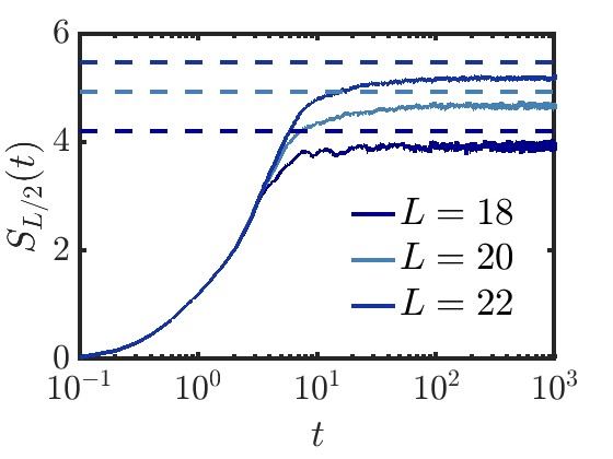
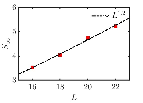
(a)(b)

Figure 11: (a-b) Growth of entanglement entropy with time for three different system sizes, $L=18,20$ and $22$ with OBC, starting from the Neel state, $101010\cdots$. In all three cases, the entanglement entropy quickly saturates to a volume law as shown in Fig. (b), which is much smaller than the thermal value of the entropy for the full system, $S_{page}=(L\ln 2-1)/2$. The saturation values for all three cases are very close to the entanglement for a random initial state on the Hilbert space within largest fragment, depicted by the three dashed lines in Fig. (a).

VI Correlated-hopping model as the large interaction limit of a $t-V$ model

In this section, we will show that our correlated-hopping model involving terms with four consecutive sites can be obtained by taking a particular large interaction limit of a model of spinless fermions. We consider a model with a nearest-neighbor hopping which we will set equal to 1, and nearest-neighbor density-density interaction terms and on-site potentials which repeat with a periodicity of four.

We consider the Hamiltonian

$$H_{4} = \sum_{j}~{}[~{}c_{j}^{\dagger}c_{j+1}~{}+~{}c_{j+1}^{\dagger}c_{j}$$ (18)

$$~{}~{}~{}~{}~{}~{}~{}~{}~{}+~{}V_{j}~{}(2n_{j}-1)~{}(2n_{j+1}-1)~{}],$$

where $V_{j}$ varies with $j$ with period four, namely, $V_{4j+1}=V_{1}$, $V_{4j+2}=V_{2}$, $V_{4j+3}=V_{3}$ and $V_{4j+4}=V_{4}$. We now consider various correlated-hopping processes involving four consecutive sites, namely, $1101\leftrightarrow 1011$, $0100\leftrightarrow 0010$, $1100\leftrightarrow 1010$ and $0101\leftrightarrow 0011$, for two different interaction patterns which are related to each other through translation by one site. We list the energy costs for the left and right sides of these correlated-hopping processes in the limit $V_{1},~{}V_{2},~{}V_{3},~{}V_{4}\rightarrow\infty$ in Table 4. We see from that table that the interaction energy costs will be equal for the left hand and right hand sides of the processes in rows 3, 4, 6 and 7 (where the occupation numbers $n_{j}$ are unequal on the first and fourth sites) if $V_{1}=-V_{3}=V$ and $V_{2}=-V_{4}=V^{\prime}$. Simultaneously, the interaction energies will not be equal for the left hand and right hand sides of the processes in rows 1, 2, 5 and 6 (where the occupation numbers are equal on the first and fourth sites) if $V,~{}V^{\prime}~{}\neq~{}0$. Hence, in the limit $V\to\pm\infty$ and $V^{\prime}\to\pm\infty$, hopping between sites $j+1$ and $j+2$ is allowed if and only if $n_{j}\neq n_{j+3}$. Note that $V$ and $V^{\prime}$ can differ from each other in general.

Our analysis thus puts forward an experimentally realizable model which reduces to the four-site correlated-hopping model in the large interaction limit. Namely, we have to consider a model for which the Hamiltonian is given by Eq. (18), with

$$V_{4j+1} = -~{}V_{4j+3}~{}=~{}V,$$

$${\rm and}~{}~{}~{}~{}V_{4j+2} = -~{}V_{4j+4}~{}=~{}V^{\prime}.$$ (19)

Before ending this section we would like to point out that our correlated-hopping model can emerge as an effective Hamiltonian due to an interplay between dynamical localization, resonance and interactions in a periodically driven system with onsite potential with spatial periodicity of four sites Aditya and Sen (2023).

Pattern of	Correlated-hopping	Energy cost for left hand side of	Energy cost for right hand side of
$V_{j}$	process	the process in the second column	the process in the second column
$V_{1}\,V_{2}\,V_{3}\,V_{4}$	$1101~{}\leftrightarrow~{}1011$	$V_{1}-V_{2}-V_{3}$	$-~{}V_{1}-V_{2}+V_{3}$
$V_{1}\,V_{2}\,V_{3}\,V_{4}$	$0100~{}\leftrightarrow~{}0010$	$-~{}V_{1}-V_{2}+V_{3}$	$V_{1}-V_{2}-V_{3}$
$V_{1}\,V_{2}\,V_{3}\,V_{4}$	$1100~{}\leftrightarrow~{}1010$	$V_{1}-V_{2}+V_{3}$	$-~{}V_{1}-V_{2}-V_{3}$
$V_{1}\,V_{2}\,V_{3}\,V_{4}$	$0101~{}\leftrightarrow~{}0011$	$-~{}V_{1}-V_{2}-V_{3}$	$V_{1}-V_{2}+V_{3}$
$V_{2}\,V_{3}\,V_{4}\,V_{1}$	$1101~{}\leftrightarrow~{}1011$	$V_{2}-V_{3}-V_{4}$	$-~{}V_{2}-V_{3}+V_{4}$
$V_{2}\,V_{3}\,V_{4}\,V_{1}$	$0100~{}\leftrightarrow~{}0010$	$-~{}V_{2}-V_{3}+V_{4}$	$V_{2}-V_{3}-V_{4}$
$V_{2}\,V_{3}\,V_{4}\,V_{1}$	$1100~{}\leftrightarrow~{}1010$	$V_{2}-V_{3}+V_{4}$	$-~{}V_{2}-V_{3}-V_{4}$
$V_{2}\,V_{3}\,V_{4}\,V_{1}$	$0101~{}\leftrightarrow~{}0011$	$-~{}V_{2}-V_{3}-V_{4}$	$V_{2}-V_{3}+V_{4}$

Table 4: Energy costs arising from the $V_{j}$ term in Eq. (18) for the left and right sides of various correlated-hopping processes for two sets of patterns of $V_{j}$ related to each other through translation by one site in the limit $V_{1}$, $V_{2}$, $V_{3}$, $V_{4}\rightarrow\infty$.

VII Comparison with a different model showing Hilbert space fragmentation

It is interesting to contrast various results for our model and a different model showing HSF which has been studied extensively De Tomasi et al. (2019); Moudgalya et al. (2022, 2020); Khemani et al. (2020). This is again a one-dimensional model with spinless fermions but with a Hamiltonian

$$H_{5}~{}=~{}\sum_{j}~{}[1~{}-~{}(n_{j}-n_{j+3})^{2}]\,(c_{j+1}^{\dagger}c_{j+2}+c_{j+2}^{\dagger}c_{j+1}).$$ (20)

This Hamiltonian connects the following pairs of states involving four consecutive sites,

$$1101 \leftrightarrow 1011$$

$$0100 \leftrightarrow 0010.$$ (21)

This comparison is particularly relevant for our study since this model is also a correlated-hopping model involving four consecutive sites just like ours. However, this model allows nearest-neighbor hoppings if the sites to the left and right of those two sites have equal particle numbers, unlike our model which enables nearest-neighbor hoppings if the sites to the left and right have different particle numbers. Defining $n_{j}=c_{j}^{\dagger}c_{j}$ as before, we find that there are three global symmetries: total particle number $C_{1}$, and two other quantities $C_{4}$ and $C_{5}$ given by

$$C_{1} = \sum_{j}~{}n_{j},$$

$$C_{4} = \sum_{j}~{}n_{2j}n_{2j+1},$$

$$C_{5} = \sum_{j}~{}n_{2j-1}n_{2j}.$$ (22)

We now observe that this model can also be mapped to a model with a Hamiltonian which involves three consecutive sites. Upon doing the mapping in Eq. (4), we obtain a model where only the following transitions are allowed,

$$110~{}\leftrightarrow~{}011.$$ (23)

The Hamiltonian of this model is

$$H_{6}~{}=~{}\sum_{j}n_{j+1}~{}(d_{j}^{\dagger}d_{j+2}~{}+~{}d_{j+2}^{\dagger}d_{j}),$$ (24)

where $n_{j}=d_{j}^{\dagger}d_{j}$. This Hamiltonian is number conserving, unlike the Hamiltonian in Eq. (6). Note, however, that the total particle numbers $\sum_{j}n_{j}$ for the models in Eqs. (20) and (24) are not related to each other in any simple way.

It turns out that a transition of the form given in Eq. (23) was studied many years ago in a classical model of diffusing dimers undergoing Markov evolution Menon et al. (1997). In that work, a complete solution for the numbers and sizes of fragments was found. For large system sizes, it was shown that the number of fragments grows exponentially as $\tau^{L}$. The number of frozen sectors is also found to grow as $\tau^{L}$, Aditya and Sen (2023) unlike our model where it grows as $1.466^{L}$. Further, it was shown in Ref. Menon et al., 1997 that for a system with OBC, the different fragments can be characterized uniquely by the numbers of three kinds of short strings, namely, $N_{A}$ strings given by $11$, $N_{B}$ given by $10$, and $N_{C}$ given by $0$. The number of states in a fragment $(N_{A},N_{B},N_{C})$ was shown to be

$$D_{N_{A},N_{B},N_{C}}~{}=~{}\frac{(N_{A}~{}+~{}N_{B}~{}+~{}N_{C})!}{N_{A}!~{}(N_{B}~{}+~{}N_{C})!}.$$ (25)

For a system with $L$ sites, we must have $2N_{A}+2N_{B}+N_{C}=L$. The filling fraction of particles is given by $(2N_{A}+N_{B})/L$. The frozen fragments with $D_{N_{A},N_{B},N_{C}}=1$ correspond to either $N_{A}=0$ and $2N_{B}+N_{C}=L$, or $N_{A}=L/2$ and $N_{B}=N_{c}=0$ (i.e., a string of $L$ $1$’s).

We can now find how the number of states in an arbitrary fragment grows with $L$. We define

$$\alpha~{}=~{}\frac{N_{A}}{L},~{}~{}~{}~{}~{}~{}\beta~{}=~{}\frac{N_{B}}{L},~{}~{}~{}~{}~{}~{}\gamma~{}=~{}\frac{N_{C}}{L}.$$ (26)

These parameters satisfy $\alpha,~{}\beta,~{}\gamma~{}\geq~{}0$, and $2\alpha+2\beta+\gamma=1$. Eliminating $\beta$, we see that the parameters $(\alpha,\gamma)$ lie in a triangular region which is bounded by the lines $\alpha=0$, $\gamma=0$ and $2\alpha+\gamma=1$ (where $\beta=0$). We now consider the limit $L\to\infty$ holding $\alpha,~{}\beta,~{}\gamma$ fixed. Using Eq. (25) and Stirling’s approximation, we find that the number of states grows as $\mu^{L}$, where $\mu$ is a function of $\alpha,~{}\gamma$ given by

$$\mu(\alpha,\gamma)~{}=~{}\frac{(\frac{1}{2}~{}+~{}\frac{\gamma}{2})^{(1+\gamma)/2}}{\alpha^{\alpha}~{}(\frac{1}{2}~{}+~{}\frac{\gamma}{2}~{}-~{}\alpha)^{(1+\gamma-2\alpha)/2}}.$$ (27)

We thus see that $\mu(\alpha,\gamma)$ varies continuously over the triangular region. The minimum value of $\mu(\alpha,\gamma)$ is equal to 1; this occurs on the line $(\alpha=0,0\leq\gamma\leq 1)$, and at the point $(\alpha=1/2,\gamma=0)$. We will now find the maximum value of $\mu(\alpha,\gamma)$. A numerical search shows that $\mu(\alpha,\gamma)$ attains its maximum on the line $2\alpha+\gamma=1$. On that line, Eq. (27) simplifies to

$$\mu(\alpha)~{}=~{}\frac{(1~{}-~{}\alpha)^{1-\alpha}}{\alpha^{\alpha}~{}(1~{}-~{}2\alpha)^{1-2\alpha}},$$ (28)

where $0\leq\alpha\leq 1/2$. We find analytically that this has a maximum at

$$\alpha~{}=~{}\frac{1}{2}~{}(1~{}-~{}\frac{1}{\sqrt{5}})~{}\simeq~{}0.2764,$$ (29)

where $\mu=\tau$. The filling fraction at this point is $2\alpha\simeq 0.5528$.

Finally, we study if there is a $t-V$ model similar to the one discussed in Sec. VI which reduces to Eq. (20) in the large interaction limit. We consider a model of the form

$$H_{7}~{}=~{}\sum_{j}~{}[~{}c_{j}^{\dagger}c_{j+1}~{}+~{}c_{j+1}^{\dagger}c_{j}~{}+~{}V_{j}~{}n_{j}~{}n_{j+1}],$$ (30)

where we again take $V_{j}$ to vary with $j$ with period four. We carry out an analysis of the energy costs for the left and right hand sides of Eq. (21) similar to the one shown in Table 4. We then find that the energy costs on the two sides of Eq. (21) are equal if $V_{1}=V_{3}=V$ and $V_{2}=V_{4}=V^{\prime}$, where $V,~{}V^{\prime}$ are independent parameters. (The interactions $V_{j}$ then have a period-two structure rather than period-four). In the limit $V\to\pm\infty$ and $V^{\prime}\to\pm\infty$, hopping between sites $j+1$ and $j+2$ will be allowed if and only if $n_{j}=n_{j+3}$.

Finally, we note that if $V=V^{\prime}$, i.e., $V_{j}=V$ for all $j$, the model in Eq. (30) becomes the standard $t-V$ model, and it is exactly solvable by the Bethe ansatz for a system with PBC Sutherland (2004). However, if $V\neq V^{\prime}$, it is not known if the model is exactly solvable.

VIII Discussion

We begin by summarizing our main results. We studied a one-dimensional correlated-hopping model of spinless fermions with terms involving four consecutive sites having a few global symmetries. This can be mapped to an assisted pair-flipping model with terms involving three consecutive sites. We found that this model shows strong HSF in a particle number basis, and evolution starting from an arbitrary basis state does not always lead to thermalization. In characterizing the HSF in this model, we found it useful to define IS, analogous to the constructions used earlier Menon et al. (1997); Menon and Dhar (1995). The IS provide us with an exponentially large number of conserved quantities which completely characterize the structure of the HSF. Using IS, we determined the total number of fragments, the number of frozen states, and the growth of the dimension of the largest fragment with the system size. These results were also verified using the transfer matrix methods and explicit enumerations.

We found that the energy level spacing distribution of the eigenspectrum is approximately Poisson, but the Hamiltonian within the largest fragment shows approximately GOE level statistics. Our study of infinite-temperature autocorrelation functions and entanglement dynamics also indicated the non-thermal behavior of our model. Further, the finite-size Mazur bound analysis of infinite-temperature autocorrelation functions at one end and inside the bulk of the system pointed towards a thermal bulk spectrum with non-thermal boundary behavior. We also compare our results with another correlated-hopping model involving four consecutive sites, which has been extensively studied in the context of HSF. Finally, we showed how this correlated-hopping model can be realized in an experimental setting using a variant of the $t-V$ model of spinless fermions in a particular limit.

In brief, we have considered a model in which the basis states are products of local finite-dimensional Hilbert spaces. In this basis, the Hamiltonian has a block diagonal structure, due to the existence of an infinite number of conserved quantities given by IS. In each fragment, the expectation values of local observables for eigenstates at a particular energy tend to the equilibrium values within that fragment. With this understanding, even frozen fragments which include a single eigenstate of the Hamiltonian are not exceptional, but are fully in conformity with the above statement.

We end by suggesting possible directions for future research. It would be useful to determine exactly how fast different fragments grow with system size for an arbitrary filling fraction in our model, similar to Eq. (25) which is known for the diffusing dimer model Menon et al. (1997). The transport properties vary significantly in different fragments, and it would be useful to understand this better Bastianello et al. (2022); Brighi et al. (2023); Wang and Yang (2023); Barma and Dhar (1994b). The behaviors of bulk and boundary autocorrelation functions for a typical random thermal state in the thermodynamic limit Hart (2023). Finally, it would be useful to study the effects of disorder De Tomasi et al. (2019); Herviou et al. (2021) and dissipation Ghosh et al. (2024) in this model. It would also be interesting to see if the concept of IS can be generalized to models where HSF occurs in an entangled basis rather than in a product state in the particle number basis.

We expect that our results can be experimentally tested in cold-atom platforms Bloch et al. (2008); Kohlert et al. (2021) where spinless fermionic chains with spatially periodic potentials and strong interactions can be realized. Recently, thermalization in some particular fragments of a model with HSF has been observed in a Rydberg atom system in one dimension Zhao et al. (2024). Another observation of HSF has been reported in a superconducting processor in a system exhibiting Stark many-body localization Wang et al. (2024).

Acknowledgments

S.A. thanks MHRD, India for financial support through a PMRF. D.S. thanks SERB, India for funding through Project No. JBR/2020/000043.

Appendix A Calculation of number of fragments

In this Appendix, we will show how the number of fragments can be calculated using a transfer matrix method. As we have discussed earlier, IS cannot contain the substrings of $1111$ and $010$. This leads us to construct the following $8\times 8$ transfer matrix $T(C_{i},C_{j})$ in which the rows and columns $C_{i}$ and $C_{j}$ denote configurations of three consecutive sites labelled as $111$, $110$, $101$, $100$, $011$, $010$, $001$ and $000$. We then have

$$T=\left(\begin{matrix}0&1&0&0&0&0&0&0\\ 0&0&1&1&0&0&0&0\\ 0&0&0&0&1&0&0&0\\ 0&0&0&0&0&0&1&1\\ 1&1&0&0&0&0&0&0\\ 0&0&0&0&0&0&0&0\\ 0&0&0&0&1&0&0&0\\ 0&0&0&0&0&0&1&1\end{matrix}\right).$$ (31)

The eigenvalues of $T$ are analytically found to be $\tau$, $-1/\tau$, $\pm i$ and $0$ (which has an algebraic multiplicity of 4), where $\tau=(\sqrt{5}+1)/2\simeq 1.618$ is the golden ratio. (The four non-zero eigenvalues are the roots of the quartic equation $z^{4}-z^{3}-z-1=0$).

Table 1 shows that $M(n)=M(n-1)+M(n-2)$ for $n\geq 4$. We can use this recursion relation to show that

$$M(n)~{}=~{}\tau^{n+1}+\left(-\frac{1}{\tau}\right)^{n+1},$$ (32)

for $n\geq 2$. (Note that only two of the non-zero eigenvalues of $T$ appear in Eq. (32)). In fact, Eq. (32) holds even for $n=0$. But for $n=1$, the right hand side of Eq. (32) gives $3$, while a simple counting shows that $M(1)$ is equal to $2$. We now define the generating function for $M(n)$ as

$$G(z)=\sum_{n=0}^{\infty}M(n)z^{n}.$$ (33)

Using the values of $M(n)$ given above, and summing the series in Eq. (33) we obtain

$$G(z)~{}=~{}\frac{\tau}{1-z\tau}-\frac{1}{\tau+z}-z.$$ (34)

Given the values of $M(n)$ in Table 1 and Eq. (32), we find that the number of fragments for a system with $L$ sites and OBC is

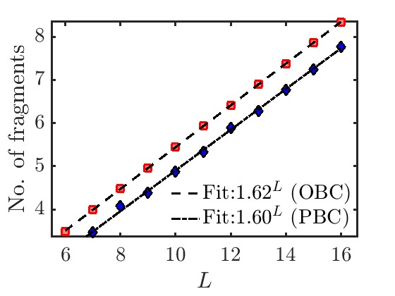
Figure 12: Number of fragments (on a log scale) versus $L$ for OBC and periodic boundary condition (PBC). The numerical fittings show that the numbers grow approximately as $1.62^{L}$ and $1.60^{L}$ for OBC and PBC, respectively.

In Fig. 12, we plot the number of fragments $N_{frag}$ versus $L$ for both OBC and PBC. In both cases, we see that $N_{frag}$ grows exponentially as $1.62^{L}$ and $1.60^{L}$, which are consistent with the analytically estimated value of $\tau^{L}$ for OBC.

We note that in our numerical work, positive random hoppings uniformly distributed in the range $[1,2]$ have been used while counting the total number of fragments with PBC in order to avoid any accidental cancellations of sums of matrix elements of the Hamiltonian. As an example of an accidental cancellation, consider $L=4$ with PBC. Then the state $|1010\rangle$ (which denotes the occupation numbers at sites $1,~{}2,~{}3,~{}4$) can go to $|1111\rangle$ in two possible ways, by the action of either $n_{3}d_{2}^{\dagger}d_{4}^{\dagger}$ or $n_{1}d_{4}^{\dagger}d_{2}^{\dagger}$. These two terms cancel each other due to the anticommutation relation $d_{2}^{\dagger}d_{4}^{\dagger}+d_{4}^{\dagger}d_{2}^{\dagger}=0$, which would imply that $|1010\rangle$ and $|1111\rangle$ belong to different fragments.

Appendix B Calculation of number of frozen states

In this Appendix, we will show how the number of frozen states can be calculated. Unlike the matrix $T$ defined in Eq. (31) which is designed to remove the configurations $010$ and $1111$, we now need to remove the configurations $010$ and $111$ in order to find states which are not connected to any other states (and are therefore frozen). We find that the required transfer matrix is a $4\times 4$ matrix whose rows and columns are labelled as $11,~{}10,~{}01$ and $00$. The required matrix is then

$$T_{1}~{}=~{}\left(\begin{array}[]{cccc}0&1&0&0\\ 0&0&1&1\\ 1&0&0&0\\ 0&0&1&1\end{array}\right).$$ (35)

We discover that one of the eigenvalues of $T_{1}$ is zero, while the other three are solutions of the cubic equation

$$\lambda^{3}-\lambda^{2}-1=0.$$ (36)

The solutions of this equation are given by

$$\lambda~{}=~{}\frac{1}{3}~{}+~{}\frac{2}{3}~{}\cos~{}\left[\frac{1}{3}\cos^{-1}\left(\frac{29}{2}\right)~{}-~{}\frac{2\pi k}{3}\right],$$ (37)

where $k$ can take the values $0,~{}1,~{}2$. We then find the three eigenvalues to be $1.466$ and $-0.233\pm 0.793i$ approximately; the magnitudes of the last two eigenvalues are less than 1. Hence, We note that this grows more slowly than than the total number of fragments which grows as $1.618^{L}$.

The number of frozen states can also be counted using the fact that the number of such states, $N_{frozen}(L)$, with OBC is given by the sum of all the matrix elements of $T_{1}^{L-2}$, for $L\geq 3$. Defining $Y=T_{1}^{L-2}$, we have

$$N_{frozen}~{}=~{}\sum_{i,j=1}^{4}Y_{i,j}.$$ (38)

The counting of frozen states with PBC is slightly different since we have to take care of the constraint that the states of the four consecutive sites ($L-1,L,1,2)$ should not contain either $111$ or $010$. Therefore, defining $Y=T_{1}^{L-2}$ and taking into account this additional constraint, we find that

$$N_{frozen}(L) = Y(1,2)+Y(1,4)+Y(2,3)$$ (39)

$$+Y(3,1)+Y(3,2)+Y(3,4)$$

$$+Y(4,1)+Y(4,3)+Y(4,4).$$

The number of frozen states for first few system sizes shown in Table 3 exactly agree with the numerically obtained numbers. We note again that for PBC, we have used random hoppings which are uniformly distributed in the range $[1,2]$ to numerically compute the number of frozen states to avoid any accidental cancellations between different matrix elements of the Hamiltonian.

Appendix C Calculation of the dimension of the largest fragment of the three-spin model

We have seen that there are exponentially many frozen fragments which have only one state each. Fragments containing $n$ blinkers have dimension $2^{n}$. However, there are other fragments which are much larger in size. We typically find that larger fragments correspond to IS with shorter length. We will now study the largest fragments whose IS turn out to consist of either the null string ($\phi$), 1, $11$ or $111$.

We will use the method of enumerative combinatorics of characters Graham et al. (1994); Menon and Dhar (1995); Menon et al. (1997); Barma and Dhar (1994a) to evaluate the dimension of the fragment of the three-spin model with OBC whose IS consists of only $\phi$ or 1’s. For clarity, we will use the symbols $A$ and $B$, rather than $0$ and $1$, to denote the two characters.

We define four formal infinite sums, $U_{0}$, $U_{1}$, $U_{2}$ and $U_{3}$ as sums of all distinct strings made of characters $A$ and $B$ that correspond to IS which can be $\phi$, $B$, $B^{2}$ or $B^{3}$, respectively. We assign a weight $x$ and $y$ to each occurrence of $A$ and $B$, and the weight of a string having $p$ number of $B$’s and $q$ number of $A$’s is $x^{p}\,y^{q}$. We denote the sum of weights of these formal series by $U_{0}(x,y)$, $U_{1}(x,y)$, $U_{2}(x,y)$ and $U_{3}(x,y)$.

In the sum of terms $U_{0}(x,y)$, there are terms is which contain no $A$’s and only $4r$ $B$’s, and other terms, which have an even number of $A$’s, must have the following structure:

$$U_{0}~{}=~{}\frac{\phi}{1-B^{4}}~{}+\sum_{r=0,1,2,3}\sum_{X}~{}\frac{B^{r}}{1-B^{4}}~{}AWA~{}X,$$ (40)

where $W$ is the sum over all possible substrings of between $A$’s that reduce to $B$, so that $AWA$ reduces to $ABA$ and therefore to $B^{3}$. Moreover, $X$ must be reducible to $B^{s}$ such that $r+3+s\equiv 0$ mod 4. Then writing different possibilities of $r$ mod 4 explicitly, we obtain

$$U_{0} = \frac{\phi}{1-B^{4}}~{}+~{}\frac{\phi}{1-B^{4}}~{}AWA~{}U_{1}$$ (41)

$$+~{}\frac{B}{1-B^{4}}~{}AWA~{}U_{0}~{}+~{}\frac{B^{2}}{1-B^{4}}~{}AWA~{}U_{3}$$

$$+~{}\frac{B^{3}}{1-B^{4}}~{}AWA~{}U_{2}.$$

Then the generating function $U_{0}$ in Eq. (41) is given by

$$U_{0}(x,y) = \frac{1}{1-x^{4}}~{}+~{}\frac{y^{2}}{1-x^{4}}~{}W(x,y)\,U_{1}(x,y)$$ (42)

$$+~{}\frac{xy^{2}}{1-x^{4}}~{}W(x,y)\,U_{0}(x,y)$$

$$+~{}\frac{x^{2}y^{2}}{1-x^{4}}~{}W(x,y)\,U_{3}(x,y)$$

$$+~{}\frac{x^{3}y^{2}}{1-x^{4}}~{}W(x,y)\,U_{2}(x,y),$$

where $W(x,y)$ denotes the weight of $W$. Since $AWA$ must reduce to $B^{3}$, it must contain an even number of $A$’s, and $y^{2}W(x,y)$ must have terms of the form $x^{r}y^{2s}$ where $r+2s=3$ mod 4, $r\geq 1$, and $s\geq 1$. Hence we can write

$$y^{2}W(x,y)=xy^{2}H(x,y),$$ (43)

where $H(x,y)$ has terms of the form $x^{p}y^{2q}$ where $p+2q=0$ mod 4.

In a similar manner, one can show that the generating functions for $U_{1}(x,y)$, $U_{2}(x,y)$ and $U_{3}(x,y)$ can be written as

$$U_{1}(x,y) = \frac{x}{1-x^{4}}~{}+~{}\frac{xy^{2}}{1-x^{4}}~{}W(x,y)\,U_{1}(x,y)$$ (44)

$$+~{}\frac{y^{2}}{1-x^{4}}~{}W(x,y)\,U_{2}(x,y)$$

$$+~{}\frac{x^{3}y^{2}}{1-x^{4}}~{}W(x,y)\,U_{3}(x,y)$$

$$+~{}\frac{x^{2}y^{2}}{1-x^{4}}~{}W(x,y)\,U_{0}(x,y),$$

$$U_{2}(x,y) = \frac{x^{2}}{1-x^{4}}~{}+~{}\frac{x^{3}y^{2}}{1-x^{4}}~{}W(x,y)\,U_{0}(x,y)$$ (45)

$$+~{}\frac{x^{2}y^{2}}{1-x^{4}}~{}W(x,y)U_{1}(x,y)$$

$$+~{}\frac{xy^{2}}{1-x^{4}}~{}W(x,y)\,U_{2}(x,y)$$

$$+~{}\frac{y^{2}}{1-x^{4}}~{}W(x,y)\,U_{3}(x,y),$$

$$U_{3}(x,y) = \frac{x^{3}}{1-x^{4}}~{}+~{}\frac{y^{2}}{1-x^{4}}~{}W(x,y)\,U_{0}(x,y)$$ (46)

$$+~{}\frac{x^{3}y^{2}}{1-x^{4}}~{}W(x,y)\,U_{1}(x,y)$$

$$+~{}\frac{x^{2}y^{2}}{1-x^{4}}~{}W(x,y)\,U_{2}(x,y)$$

$$+~{}\frac{xy^{2}}{1-x^{4}}~{}W(x,y)\,U_{3}(x,y).$$

The generating functions given above can be combined as

$$V(x,y)=U_{0}(x,y)+U_{1}(x,y)+U_{2}(x,y)+U_{3}(x,y).$$ (47)

Using the identity $(1+x+x^{2}+x^{3})/(1-x^{4})=1/(1-x)$ and Eq. (43), we find that

$$V(x,y)~{}=~{}\frac{1}{1~{}-~{}x~{}-~{}xy^{2}~{}H(x,y)}.$$ (48)

We now set $y=x$. Then $U_{0},~{}U_{1},~{}U_{2},~{}U_{3}$ will become polynomials in $x$ with terms whose degrees are equal to $0,~{}1,~{}2,~{}3$ mod 4, respectively, and $H(x,y)=H(x)$ will become a polynomial in $x^{4}$. We then obtain

$$V(x) = \frac{1}{1-x-x^{3}\,H(x)},$$ (49)

where $V(x)$ is the generating function of all strings that reduce to $B$’s only, and $xH(x)$ is related to IS’s which reduce to a single $B$. By direct examination of strings of lengths $0-3$ (namely, $\phi\to 1$, $B\to x$, $BB\to x^{2}$, $BBB\to x^{3}$ and $ABA\to xy^{2}=x^{3}$ for $y=x$), we find that the first few terms in $V(x)$ and $H(x)$ are given by

$$V(x) = 1~{}+~{}x~{}+~{}x^{2}~{}+~{}2x^{3}~{}+~{}\cdots,$$

$$H(x) = 1~{}+~{}\cdots.$$ (50)

Next, we can write $V(x)$ as

$$V(x)=V_{0}(x)+x\,V_{1}(x)+x^{2}\,V_{2}(x)+\,x^{3}\,V_{3}(x),$$ (51)

where $V_{0}$, $V_{1}$, $V_{2}$ and $V_{3}$ are all polynomials in $x^{4}$. Using Eq. (49) and the fact that $V_{0}$, $V_{1}$, $V_{2}$ and $V_{3}$ are polynomials in $x^{4}$, we can show that

$$V_{0}(x) = \frac{V(x)~{}+~{}V(-x)~{}+~{}V(ix)~{}+~{}V(-ix)}{4},$$ (52)

$$= \frac{1-2x^{4}H}{(1-2x^{4}H)^{2}-x^{4}(1+x^{4}H^{2})^{2}},$$

$$V_{1}(x) = \frac{V(x)~{}-~{}V(-x)~{}-~{}iV(ix)~{}+~{}iV(-ix)}{4x},$$ (53)

$$= \frac{1-x^{4}+x^{8}\,H^{3}}{(1-2x^{4}H)^{2}-x^{4}(1+x^{4}H^{2})^{2}},$$

$$V_{2}(x) = \frac{V(x)~{}+~{}V(-x)~{}-~{}V(ix)~{}-~{}V(-ix)}{4x^{2}},$$ (54)

$$= \frac{1+x^{4}H^{2}}{(1-2x^{4}H)^{2}-x^{4}(1+x^{4}H^{2})^{2}},$$

$$V_{3}(x) = \frac{V(x)~{}-~{}V(-x)~{}+~{}iV(ix)~{}-~{}iV(-ix)}{4x^{3}},$$ (55)

$$= \frac{1+H-x^{4}\,H^{2}}{(1-2x^{4}H)^{2}-x^{4}(1+x^{4}H^{2})^{2}}.$$

Next, we can show that $V_{3}(x)=2V_{2}(x)$ as follows.

1. Given a string in $V_{2}$, one can add a $1$ to the left to obtain a string in $V_{3}$. Further, this process is reversible, i.e., given a string in $V_{3}$ beginning with $1$, one can delete the 1 to obtain a string in $V_{2}$.

2. Next, given a string belonging to $V_{2}$ that begins with a $0$, one can add a 1 on the right side of the string to obtain a string in $V_{3}$. This process is also reversible: given a string in $V_{3}$ which begins with a 0 and ends with a 1, we can delete the 1 to obtain a string in $V_{2}$ which begins with a 0.

3. Finally, given a string in $V_{2}$, that begins with a 1, we can replace the 1 by a 0 and add a 0 at the right end of the string. This procedure thus produces a string in $V_{3}$. This mapping is again reversible similar to rules 1 and 2.

Taking $V_{3}=2V_{2}$ into account and using Eq. (54) and (55), we get the following quadratic equation for $H(x)$

$$3x^{4}\,H^{2}-H+1 = 0\,,$$

$${\rm which~{}implies}~{}~{}~{}H(x) = \frac{1~{}\pm~{}\sqrt{1-12x^{4}}}{6x^{4}}.$$ (56)

Eq. (50) tells us that we have to take the lower sign (minus) in the expression for $H(x)$ in Eq. (56). We then obtain the final expression

$$V(x)=\frac{1}{1~{}-~{}x~{}-~{}\left(\frac{1~{}-~{}\sqrt{1-12x^{4}}}{6x}\right)}.$$ (57)

This is Eq. (12) in the main text.

Appendix D Comparison between the growths of the largest fragments in four-site and three-site models

In this section, we compare the dimensions of the fragments generated from the root state, $1010\cdots 10$ (or $0101\cdots 01$) of the four-site model with the one generated from the root state, $111\cdots 111$ of the three-site model. Note that both the states $1010\cdots 10$ and $0101\cdots 01$ of the four-site model map to the same state, $111\cdots 111$, of the three-site model under bond-site mapping. We first we compare the cases with OBC. As evinced in Table 5, the dimensions of fragments originating from either of the root states $1010\cdots 10$ and $0101\cdots 01$ of the four-site model with $L$ sites are exactly the same as the one obtained from the root state $111\cdots 111$ of the three-site model with $L-1$ sites. This can be anticipated from the fact that the bond-site mapping mentioned in Sec. II maps two states of the four-site model with $L$ sites to a single state of the three-site model with $L-1$ sites with OBC.

$L$	$~{}D^{\text{four-site}}_{L}~{}$	$~{}D^{\text{three-site}}_{L}~{}$
3	1	2
4	2	3
5	3	4
6	4	6
7	12	12
8	12	19
9	19	28
10	28	46
11	46	92
12	92	150
13	150	232
14	232	396
15	396	792
16	792	1315
17	1315	2092
18	2092	3646
19	3646	7292
20	7292	12258
21	12258	19864
22	19864	35076
23	35076	70152
24	70152	118990

Table 5: Dimensions of fragments generated from the root states $1010\cdots 10$ (or $0101\cdots 01$) and $111\cdots 11$ for the four-site and three-site models respectively, with OBC. We observe two fragments of identical dimensions of the four-site model with $L$ sites maps to a single fragment originated from the root state $1111\cdots 11$ of the three-site model with $L-1$ sites.

Next, we compare the fragment sizes for the four-site and three-site models with PBC. We will assume that the system size $L$ is even to take the periodicity of the four-site model into account. As shown in Table 6, the dimension of the fragment for the root state $1010\cdots 10$ (or $0101\cdots 01)$ of the four-site model is two times larger than that of the three-site model for the root state $111\cdots 11$ for $L=4n$. This is due to the fact that the global symmetries $C_{2}$ and $C_{3}$ of the four-site model, as discussed in Eq. (3), are well-defined for $L=4n$, and hence, the states $1010\cdots 10$ and $0101\cdots 01$ lie in the same symmetry sector and belong to a single fragment for a system with PBC. On the other hand, we find that two different fragments arise from the root states $1010\cdots 10$ and $0101\cdots 01$ in the four-site model whose dimensions are the same as the single fragment of the three-site model for a chain with $L=4n+2$ sites with PBC. We also note that the two root states of the four-site model are not connected to each other by the global symmetries $C_{2}$ and $C_{3}$ for $L=4n+2$, and therefore they generate two different fragments of identical sizes.

$L$	$~{}D^{\text{four-site}}_{L}~{}$	$~{}D^{\text{three-site}}_{L}~{}$
4	6	3
6	10	10
8	38	19
10	106	106
12	300	150
14	1156	1156
16	2630	1315
18	12826	12826
20	24516	12258
22	143980	143980
24	237980	118990
26	1630084	1630084

Table 6: Dimensions of fragments generated from the root configurations $1010\cdots$ (or $0101\cdots 01$) and $111\cdots 111$ for the four-site and three-site model, respectively, with PBC. We note that for $L=4n$, the two states belong to the same fragment in the four-site model, whereas for $L=4n+2$, the four-site model exhibits two different fragments with the same size $D_{L}$, one coming from the root configuration $101010\cdots 10$ and the other from $010101\cdots 01$.

Appendix E Fragmentation structure of the four-site model away from half-filling

$L$	6	12	18	24
$D_{i,L}$	7	107	1906	35259

Table 7: Dimension of the fragment $D_{i,L}$ versus $L$ obtained from the root state $101000101000\cdots$ for the three-site model with OBC.

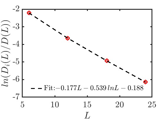
Figure 13: Plot of the ratio of the dimension $D_{i}$ of the fragment of interest to the total dimension $D=2^{L}$ of the Hilbert space (shown on a log scale) versus $L$ for a system with with OBC. The ratio is seen to decrease exponentially with $L$.

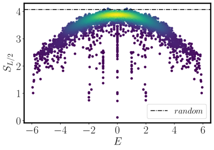
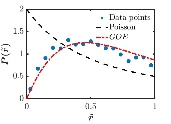
(a)(b)

Figure 14: (a) Plot of $S_{L/2}$ versus $E$ for the fragment generated from the root state, $0111001110\cdots$ for $L=24$ at filling fraction $\nu=2/3$ for the four-site model with OBC. The fragment size is $4906$. The dash-dot line indicates the value of the entanglement entropy of a random state in the full Hilbert space within this subspace. The entanglement spectrum contains a small fraction of eigenstates with low entanglement entropy in the middle of the spectrum. (b) The level spacing ratio analysis for the same fragment in the presence of a small uniformly distributed random disorder with disorder strength $w=0.01$. The probability distribution of $\tilde{r}$ is close to the GOE distribution with $\langle\tilde{r}\rangle\simeq 0.51$.

We will discuss here strong HSF away from half-filling in our model. In doing so, we consider the following root states of the four-site model with OBC, $\cdots 011110011110\cdots$ or $\cdots 10001100001\cdots$ which correspond to filling fractions $\nu=2/3$ and $1/3$ respectively. Both these states map to the state $\cdots 101000101000\cdots$ in the three-site model with OBC. Taking this state as a root configuration of the three-site model, we find the dimension of this Hilbert space fragment by numerical enumeration for $L=6,~{}12,~{}18$ and $24$; the results are shown in Table  7. We have chosen the system sizes to be multiples of 6 to ensure that the pattern of the root state remains invariant as the system size is increased.

In Fig. 13, we show how this fragment grows with $L$ by the numerical enumeration method. Moreover, the numerical fitting indicates that dimension of this particular fragment grows as $1.68^{L}/L^{0.54}$. This again implies that $D_{i}/D$ goes to zero for $L\rightarrow\infty$, where $D$ being the total dimension of the Hilbert space, which indicates strong HSF Sala et al. (2020). This observation leads us to conclude that our four-site model exhibits strong HSF Sala et al. (2020) at arbitrary filling fractions.

In Figs. 14 (a-b), we show the half-chain entanglement entropy as a function of the energy $E$ for the fragment generated from the root state $011110011110\cdots$ at $\nu=2/3$ for the four-site model with $L=24$ and OBC; the dimension of this fragment is $4906$. The spectrum shows that most of the eigenstates lie close to a single curve as in a thermal system. Nevertheless, there is also a small fraction of states in the middle of the spectrum with anomalously low entanglement entropy. We further perform an analysis of the energy level statistics within this fragment after adding a small amount of randomly distributed on-site disorder of strength $w=0.01$ for the same reasons mentioned in Sec. IV. The probability distribution of $\tilde{r}$ within this fragment is found to follow the GOE with $\langle\tilde{r}\rangle\simeq 0.51$, which is close to the GOE value. The fluctuations in the analysis of $\tilde{r}$ arise due to the limited system sizes. Since we want to keep the $01110$ pattern of the root state intact while generating this sector, we must take $L$ to be a multiple of six. We have to limit our analysis to $L=24$ since the next system size $L=30$ is numerically very difficult. We find that our model always exhibits strong HSF irrespective of the filling unlike models where a transition from strong to weak HSF can occur as a function of the filling fraction Morningstar et al. (2020); Wang and Yang (2023).

References

- Srednicki (1994) M. Srednicki, Phys. Rev. E 50, 888 (1994).
- Deutsch (1991) J. M. Deutsch, Phys. Rev. A 43, 2046 (1991).
- Rigol et al. (2008) M. Rigol, V. Dunjko, and M. Olshanii, Nature 452, 854 (2008).
- Polkovnikov et al. (2011) A. Polkovnikov, K. Sengupta, A. Silva, and M. Vengalattore, Rev. Mod. Phys. 83, 863 (2011).
- Rigol et al. (2007) M. Rigol, V. Dunjko, V. Yurovsky, and M. Olshanii, Phys. Rev. Lett. 98, 050405 (2007).
- Fagotti and Essler (2013) M. Fagotti and F. H. L. Essler, Phys. Rev. B 87, 245107 (2013).
- Ikeda et al. (2013) T. N. Ikeda, Y. Watanabe, and M. Ueda, Phys. Rev. E 87, 012125 (2013).
- Caux and Konik (2012) J.-S. Caux and R. M. Konik, Phys. Rev. Lett. 109, 175301 (2012).
- Mussardo (2013) G. Mussardo, Phys. Rev. Lett. 111, 100401 (2013).
- Pal and Huse (2010) A. Pal and D. A. Huse, Phys. Rev. B 82, 174411 (2010).
- Vosk and Altman (2013) R. Vosk and E. Altman, Phys. Rev. Lett. 110, 067204 (2013).
- Huse et al. (2013) D. A. Huse, R. Nandkishore, V. Oganesyan, A. Pal, and S. L. Sondhi, Phys. Rev. B 88, 014206 (2013).
- Nandkishore and Huse (2015) R. Nandkishore and D. A. Huse, Annual Review of Condensed Matter Physics 6, 15 (2015).
- Iadecola and Schecter (2020) T. Iadecola and M. Schecter, Phys. Rev. B 101, 024306 (2020).
- Turner et al. (2018) C. J. Turner, A. A. Michailidis, D. A. Abanin, M. Serbyn, and Z. Papić, Nature Physics 14, 745 (2018).
- Choi et al. (2019) S. Choi, C. J. Turner, H. Pichler, W. W. Ho, A. A. Michailidis, Z. Papić, M. Serbyn, M. D. Lukin, and D. A. Abanin, Phys. Rev. Lett. 122, 220603 (2019).
- Moudgalya et al. (2018) S. Moudgalya, N. Regnault, and B. A. Bernevig, Phys. Rev. B 98, 235156 (2018).
- Lin and Motrunich (2019) C.-J. Lin and O. I. Motrunich, Phys. Rev. Lett. 122, 173401 (2019).
- Iadecola et al. (2019) T. Iadecola, M. Schecter, and S. Xu, Phys. Rev. B 100, 184312 (2019).
- Moudgalya et al. (2022) S. Moudgalya, B. A. Bernevig, and N. Regnault, Reports on Progress in Physics 85, 086501 (2022).
- Rakovszky et al. (2020) T. Rakovszky, P. Sala, R. Verresen, M. Knap, and F. Pollmann, Phys. Rev. B 101, 125126 (2020).
- Moudgalya and Motrunich (2022) S. Moudgalya and O. I. Motrunich, Phys. Rev. X 12, 011050 (2022).
- Moudgalya et al. (2020) S. Moudgalya, B. A. Bernevig, and N. Regnault, Phys. Rev. B 102, 195150 (2020).
- Sala et al. (2020) P. Sala, T. Rakovszky, R. Verresen, M. Knap, and F. Pollmann, Phys. Rev. X 10, 011047 (2020).
- Brighi et al. (2023) P. Brighi, M. Ljubotina, and M. Serbyn, SciPost Phys. 15, 093 (2023).
- De Tomasi et al. (2019) G. De Tomasi, D. Hetterich, P. Sala, and F. Pollmann, Phys. Rev. B 100, 214313 (2019).
- Khemani et al. (2020) V. Khemani, M. Hermele, and R. Nandkishore, Phys. Rev. B 101, 174204 (2020).
- Yang et al. (2020) Z.-C. Yang, F. Liu, A. V. Gorshkov, and T. Iadecola, Phys. Rev. Lett. 124, 207602 (2020).
- Lee et al. (2021) K. Lee, A. Pal, and H. J. Changlani, Phys. Rev. B 103, 235133 (2021).
- Mukherjee et al. (2021) B. Mukherjee, D. Banerjee, K. Sengupta, and A. Sen, Phys. Rev. B 104, 155117 (2021).
- Khudorozhkov et al. (2022) A. Khudorozhkov, A. Tiwari, C. Chamon, and T. Neupert, SciPost Phys. 13, 098 (2022).
- Yoshinaga et al. (2022) A. Yoshinaga, H. Hakoshima, T. Imoto, Y. Matsuzaki, and R. Hamazaki, Phys. Rev. Lett. 129, 090602 (2022).
- Hart and Nandkishore (2022) O. Hart and R. Nandkishore, Phys. Rev. B 106, 214426 (2022).
- Stephen et al. (2024) D. T. Stephen, O. Hart, and R. M. Nandkishore, Phys. Rev. Lett. 132, 040401 (2024).
- Ghosh et al. (2023) S. Ghosh, I. Paul, and K. Sengupta, Phys. Rev. Lett. 130, 120401 (2023).
- Aditya and Sen (2023) S. Aditya and D. Sen, SciPost Phys. Core 6, 083 (2023).
- Zhang et al. (2023) L. Zhang, Y. Ke, L. Lin, and C. Lee, arXiv:2311.11771 (2023).
- Barma and Dhar (1994a) M. Barma and D. Dhar, Phys. Rev. Lett. 73, 2135 (1994a).
- Menon and Dhar (1995) M. K. H. Menon and D. Dhar, Journal of Physics A: Mathematical and General 28, 6517 (1995).
- Menon et al. (1997) G. I. Menon, M. Barma, and D. Dhar, Journal of Statistical Physics 86, 1237 (1997).
- Graham et al. (1994) R. L. Graham, D. E. Knuth, and O. Patashnik, Chapter 7: Generating Functions”, Concrete mathematics: a foundation for computer science., 2nd ed. (Amsterdam: Addison-Wesley Publishing Group, 1994).
- Wigner (1955) E. P. Wigner, Annals of Mathematics 62, 548 (1955).
- Serbyn et al. (2016) M. Serbyn, A. A. Michailidis, D. A. Abanin, and Z. Papić, Phys. Rev. Lett. 117, 160601 (2016).
- Mazur (1969) P. Mazur, Physica 43, 533 (1969).
- Suzuki (1971) M. Suzuki, Physica 51, 277 (1971).
- Beugeling et al. (2014) W. Beugeling, R. Moessner, and M. Haque, Phys. Rev. E 89, 042112 (2014).
- Page (1993) D. N. Page, Phys. Rev. Lett. 71, 1291 (1993).
- Atas et al. (2013) Y. Y. Atas, E. Bogomolny, O. Giraud, and G. Roux, Phys. Rev. Lett. 110, 084101 (2013).
- Berry and Tabor (1977) M. V. Berry and M. Tabor, Proceedings of the Royal Society of London. Series A, Mathematical and Physical Sciences 356, 375 (1977).
- Herviou et al. (2021) L. Herviou, J. H. Bardarson, and N. Regnault, Phys. Rev. B 103, 134207 (2021).
- Kwan et al. (2023) Y. H. Kwan, P. H. Wilhelm, S. Biswas, and S. A. Parameswaran, arXiv:2304.02669 (2023).
- Hart (2023) O. Hart, arXiv:2308.00738 (2023).
- Sutherland (2004) B. Sutherland, Beautiful Models (World Scientific, Singapore, 2004).
- Bastianello et al. (2022) A. Bastianello, U. Borla, and S. Moroz, Phys. Rev. Lett. 128, 196601 (2022).
- Wang and Yang (2023) C. Wang and Z.-C. Yang, Phys. Rev. B 108, 144308 (2023).
- Barma and Dhar (1994b) M. Barma and D. Dhar, Phys. Rev. Lett. 73, 2135 (1994b).
- Ghosh et al. (2024) S. Ghosh, K. Sengupta, and I. Paul, Phys. Rev. B 109, 045145 (2024).
- Bloch et al. (2008) I. Bloch, J. Dalibard, and W. Zwerger, Rev. Mod. Phys. 80, 885 (2008).
- Kohlert et al. (2021) T. Kohlert, S. Scherg, P. Sala, F. Pollmann, B. H. Madhusudhana, I. Bloch, and M. Aidelsburger, arXiv:2106.15586 (2021).
- Zhao et al. (2024) L. Zhao, P. R. Datla, W. Tian, M. M. Aliyu, and H. Loh, arXiv:2403.09517 (2024).
- Wang et al. (2024) Y.-Y. Wang, Y.-H. Shi, Z.-H. Sun, C.-T. Chen, Z.-A. Wang, K. Zhao, H.-T. Liu, W.-G. Ma, Z. Wang, H. Li, J.-C. Zhang, Y. Liu, C.-L. Deng, T.-M. Li, Y. He, Z.-H. Liu, Z.-Y. Peng, X. Song, G. Xue, H. Yu, K. Huang, Z. Xiang, D. Zheng, K. Xu, and H. Fan, arXiv:2403.09095 (2024).
- Morningstar et al. (2020) A. Morningstar, V. Khemani, and D. A. Huse, Phys. Rev. B 101, 214205 (2020).