Electron-positron annihilation into $K\bar{K}\pi$ and their contributions to $(g-2)_{\mu}$

Abstract

In this paper, a coherent study of the $e^{+}e^{-}$ annihilation into $K^{+}K^{-}\pi^{0}$, $K^{0}_{S}K^{0}_{L}\pi^{0}$ and $K^{0}_{S}K^{\pm}\pi^{\mp}$ is carried out within the framework of resonance chiral theory. The amplitudes are fixed by fitting to the experimental cross-section and invariant mass spectrum. With these amplitudes, one can calculate the hadronic vacuum polarization form factors of these processes. The leading order contributions of $\sigma(e^{+}e^{-}\to K\bar{K}\pi)$ to the anomalous magnetic moment of the muon, $(g-2)_{\mu}$, is obtained as $a_{\mu}^{\rm HVP,LO}(e^{+}e^{-}\to K\bar{K}\pi)=(3.07\pm 0.07)\times 10^{-10}$ up to $E_{\rm cm}=2.3$ GeV.

I Introduction

Quantum Chromodynamics (QCD) is widely accepted as the basic theory of the strong interaction, of which the running coupling constant $\alpha_{s}$ reflects the strength of the interaction among quarks and gluons. Due to the asymptotic freedom nature of $\alpha_{s}$ Gross and Wilczek (1973); Politzer (1973), i.e., $\alpha_{s}$ decreases with increasing energy, it allows people to apply perturbative QCD (pQCD) to describe strong interactions in the high energy region, $E_{\rm cm}\geq$ 2 GeV, where $E_{\rm cm}$ is the energy in the center-of-mass frame (c.m.f.). However, at low energy region, $\alpha_{s}$ becomes extremely too large to be taken as a perturbative parameter. Alternatively, one can use the effective field theory (EFT) to obtain the relevant hadronic dynamic information in the non-perturbative regime. As an effective theory of QCD in the low energy region, chiral perturbation theory (ChPT) Weinberg (1979); Gasser and Leutwyler (1984) describes the interactions between the lightest pseudoscalar mesons successfully. The Goldstone bosons arise due to chiral symmetry breaking, and they are treated as the degrees of freedom in EFT. Lorentz invariance, chiral symmetry, and discrete symmetry are implemented to construct the effective Lagrangians. ChPT has made significant achievements in studying the interactions between the lightest pseudoscalars composed of the lightest $u$, $d$, and $s$ valence quarks, but it is restricted to be applied at very low energies, e.g., $\pi\pi$ and $\pi K$ scattering around the threshold, as the power-counting is based on expansions of momenta.

In the middle energy region, both pQCD and ChPT fail to give an excellent description of the strong interaction. Further, there are many heavier resonances that appear in these regions, like vector $V(1^{--})$, axial-vector $A(1^{++})$ and $B(1^{+-})$. In the spirit of EFT, one can include these resonances as the new degrees of freedom. The chiral and discrete symmetries, i.e., the conservation of parity ($P$), charge conjugation ($C$), and hermiticity (h.c.), can still be applied to construct the interaction Lagrangians between them and the pseudoscalars. Such a success theory tool is the resonance chiral theory (RChT) Ecker et al. (1989a, b); Cirigliano et al. (2006); Portoles (2010). It works well in the energy region where the lightest resonance states appear, e.g., ${M_{\rho}\leqslant E_{\rm cm}}\lesssim 1.5$ GeV, with $M_{\rho}$ the mass of $\rho(770)$. As discussed above, RChT is a systematic theoretical tool that works in the energy region where the hadronic contribution to the anomalous magnetic moment of the muon is significant.

The muon anomalous magnetic moment, $a_{\mu}=(g-2)_{\mu}/2$, is one of the most precise indicators of new physics that can be both calculated reliably in the Standard Model (SM) and measured in experiments with very high statistics Jegerlehner (2017). Therefore, the deep understanding of $a_{\mu}$ may give a definitive answer to the question of whether there exists new physics beyond the SM or not. In 2021, the Fermilab National Accelerator Laboratory (FNAL) published an accurate experimental result on the muon anomalous magnetic moment, $a_{\mu}({\rm Exp})=116592040(54)\times 10^{-11}~{}(0.46~{}{\rm ppm})$ Abi et al. (2021). After combining the result measured by the Brookhaven National Laboratory (BNL) Bennett et al. (2006), it deviated from the theoretical prediction of SM Aoyama et al. (2020) by 4.2 $\sigma$. This reveals a possible new physics signal and draws extensive attention to particle physics. Very recently, the FNAL released their latest result in August 2023, $a_{\mu}({\rm Exp})=116592055(24)\times 10^{-11}~{}(0.20~{}{\rm ppm})$ Aguillard et al. (2023), leading to an average value of experimental measurements as $a^{\rm avg}_{\mu}({\rm Exp})=116592059(22)\times 10^{-11}~{}(0.19~{}{\rm ppm})$. Now the discrepancy between the theoretical prediction of SM and the experimental measurement reaches $\Delta a_{\mu}=a^{\rm avg}_{\mu}({\rm Exp})-a_{\mu}({\rm SM})=(249\pm 48)\times 10^{-11}$, with a significance of 5.1 $\sigma$. Nevertheless, the theoretical predictions of different models have apparent discrepancies. Unlike what is done by the data-driven method Colangelo et al. (2019); Keshavarzi et al. (2018); Davier et al. (2020); Keshavarzi et al. (2020), the lattice QCD has progressed on the study of $a_{\mu}$ and gives a much larger hadronic vacuum polarization (HVP) contribution Cè et al. (2022); Borsanyi et al. (2021); Alexandrou et al. (2023), resulting in a much closer theoretical prediction to the experimental one, i.e. a much smaller significance. Besides, it is worth mentioning that the latest measurement of the cross-section of $e^{+}e^{-}\to\pi\pi$ by CMD-3 Ignatov et al. (2023) is larger than the previous measurements, e.g. Refs. Lees et al. (2012); Anastasi et al. (2018); Ablikim et al. (2016); Xiao et al. (2018), implying a larger HVP contribution (to the theoretical $a_{\mu}$) which is close to the results of the lattice QCD.

In the theoretical predictions, the most significant uncertainties come from the HVP and the hadronic light-by-light (HLBL) scatterings, where the former has even larger uncertainties than the latter. The essential error source of HVP is from the processes of electron-positron annihilation into the lightest pseudoscalar mesons. In our previous studies Qin et al. (2021); Wang et al. (2023), we have studied the $e^{+}e^{-}$ annihilation processes to some of the two and three pseudoscalar states, i.e. $\pi\pi$, $K\bar{K}$, $\pi\gamma$, $\eta\gamma$ and $\pi\pi\pi$, $\pi\pi\eta$ within the framework of RChT, and their contributions to the $(g-2)_{\mu}$ are given. In the present analysis, we will continue to analyze the processes of $e^{+}e^{-}\to K\bar{K}\pi$ with a similar theoretical framework as before. Unlike the case of $e^{+}e^{-}\to\pi\pi\pi$, the tensor mesons appear as the intermediate states in the process of $e^{+}e^{-}\to K\bar{K}\pi$ and play an important role in the interactions with pseudoscalars, vectors, and photons. This needs further systematical study within RChT . Other than the interaction Lagrangians of one tensor coupling with two pseudoscalars (TPP) Toublan (1996); Ecker and Zauner (2007), we build all the other Lagrangians associated with one tensor, e.g. tensor electromagnetic current-pseudoscalar (TJP), tensor-vector-pseudoscalar (TVP). They are constructed in the framework of RChT, taking into account the Lorentz invariance, chiral symmetry, and discrete symmetries.

On the experimental side, the process $e^{+}e^{-}\to K\bar{K}\pi$ has been measured a few times by different collaborations, such as DM1, DM2, BABAR, SND, CMD-3, and BESIII from 1982 to 2024 Mane et al. (1982); Bisello et al. (1991); Aubert et al. (2008); Solodov et al. (2016); Lees et al. (2017); Achasov et al. (2018); Semenov et al. (2019); Achasov et al. (2020); Ablikim et al. (2022, 2024). Especially there are also measurements about two body invariant mass spectra Achasov et al. (2018, 2020), which contain the Dalitz plot information and can be somewhat helpful for refining the amplitudes Dai and Pennington (2014a, b); Yao et al. (2021). These datasets, together with the theoretical tools of RChT, provide an appropriate way to refine the analysis of the processes of $e^{+}e^{-}\to K\bar{K}\pi$.

The remaining parts of the paper are organized as follows. In section II, we will briefly introduce the theoretical framework based on RChT and construct all the required interaction Lagrangians. Then, we derive the form factors for $K\bar{K}\pi$ and discuss the high energy behavior constraints. In section III, we will show our numerical results and obtain the HVP contributions of $\sigma(e^{+}e^{-}\to K\bar{K}\pi)$. Finally, we summarize the conclusions.

II Theoretical framework

II.1 Effective Lagrangians

As mentioned above, at very low energies, ChPT describes well the interactions of pseudoscalar Goldstone bosons generated by the spontaneous breaking of chiral symmetry. These pseudoscalars ($\pi,K,\eta$) can be filled in an octet field $\Phi$, which is realized nonlinearly by the unitary matrix in the flavor space

$$u(\Phi)={\rm exp}\left\{\frac{i}{\sqrt{2}F}\Phi\right\},$$ (1)

with

$$\Phi=\left(\begin{array}[]{c c c}\frac{\pi^{0}}{\sqrt{2}}+\frac{\eta_{8}}{\sqrt{6}}&\pi^{+}&K^{+}\\ \pi^{-}&-\frac{\pi^{0}}{\sqrt{2}}+\frac{\eta_{8}}{\sqrt{6}}&K^{0}\\ K^{-}&\bar{K}^{0}&-\frac{2\eta_{8}}{\sqrt{6}}\\ \end{array}\right),$$ (5)

where $F$ is the pion decay constant, and its value is taken as $92.2$ MeV Workman et al. (2022). The physical states $\eta$ and $\eta^{\prime}$ are composed of a mixture of the octet $\eta_{8}$ and the singlet $\eta_{0}$ through the mixing angle $\theta_{P}$:

$$\binom{\eta_{8}}{\eta_{0}}=\binom{\cos\theta_{P}~{}~{}~{}~{}\sin\theta_{P}}{-\sin\theta_{P}~{}~{}\cos\theta_{P}}\binom{\eta}{\eta^{\prime}}.$$ (6)

In this analysis, $K_{S}^{0}$ and $K_{L}^{0}$ are in final states and they can be written in terms of $K^{0}-\bar{K}^{0}$ mixture, i.e., $|K_{S}^{0}\rangle=1/\sqrt{2}~{}(|K^{0}\rangle+|\bar{K}^{0}\rangle)$ and $|K_{L}^{0}\rangle=1/\sqrt{2}~{}(|K^{0}\rangle-|\bar{K}^{0}\rangle)$ with the assumption of conservation of $CP$ transformations.

In the intermediate energy regions, there appears a large number of resonances, e.g., vectors $V(\rho,\omega,\phi,K^{\ast})$ and tensors $T(a_{2}^{0},f_{2},f_{2}^{\prime},K_{2}^{\ast})$. It is difficult for ChPT to include the interactions involving these resonances, and RChT can be applied to expand the working energy region of ChPT, where the resonances are filled in the octets and singlets as

$$R=\sum_{i=1}^{8}\frac{\lambda_{i}}{\sqrt{2}}R_{i}+\frac{R_{0}}{\sqrt{3}}\mathbbm{1},$$ (7)

where $R=V,T$ denotes vector and tensor resonances, respectively. The vector mesons are described by the anti-symmetric tensor field Dai et al. (2013), which can be filled in an explicit matrix form as

$$V_{\mu\nu}\!=\!\left(\begin{array}[]{c c c}\frac{\rho^{0}}{\sqrt{2}}+\frac{\omega_{8}}{\sqrt{6}}+\frac{\omega_{0}}{\sqrt{3}}&\rho^{+}&K^{\ast+}\\ \rho^{-}&-\frac{\rho^{0}}{\sqrt{2}}+\frac{\omega_{8}}{\sqrt{6}}+\frac{\omega_{0}}{\sqrt{3}}&K^{\ast 0}\\ K^{\ast-}&\bar{K}^{\ast 0}&-\frac{2\omega_{8}}{\sqrt{6}}+\frac{\omega_{0}}{\sqrt{3}}\\ \end{array}\!\right)_{\mu\nu}\!\!\!,$$ (11)

and the tensor mesons are described by the symmetric tensor field Ecker and Zauner (2007)

$$T_{\mu\nu}\!=\!\left(\begin{array}[]{c c c}\frac{a_{2}^{0}}{\sqrt{2}}+\frac{f_{2}^{8}}{\sqrt{6}}+\frac{f_{2}^{0}}{\sqrt{3}}&a_{2}^{+}&K_{2}^{\ast+}\\ a_{2}^{-}&-\frac{a_{2}^{0}}{\sqrt{2}}+\frac{f_{2}^{8}}{\sqrt{6}}+\frac{f_{2}^{0}}{\sqrt{3}}&K_{2}^{\ast 0}\\ K_{2}^{\ast-}&\bar{K}_{2}^{\ast 0}&-\frac{2f_{2}^{8}}{\sqrt{6}}+\frac{f_{2}^{0}}{\sqrt{3}}\\ \end{array}\!\right)_{\mu\nu}\!\!\!,$$ (15)

where $V_{\mu\nu}=-V_{\nu\mu}$ and $T_{\mu\nu}=T_{\nu\mu}$. For simplicity, all states are considered to be ideal mixing if not specified. For example, the $\rho^{0}-\omega$ mixing is ignored. The octet $\omega_{8}$ and singlet $\omega_{0}$ of the vectors can be written as a linear combination of physical $\omega$ and $\phi$ resonances,

$$\omega_{8}=\sqrt{\frac{1}{3}}\omega+\sqrt{\frac{2}{3}}\phi,~{}~{}~{}\omega_{0}=\sqrt{\frac{2}{3}}\omega-\sqrt{\frac{1}{3}}\phi.$$

The mixing mechanism of the tensors is similar to the vectors. One has

$$f_{2}^{8}=\sqrt{\frac{1}{3}}f_{2}+\sqrt{\frac{2}{3}}f_{2}^{\prime},~{}~{}~{}f_{2}^{0}=\sqrt{\frac{2}{3}}f_{2}-\sqrt{\frac{1}{3}}f_{2}^{\prime}\,.$$

The interaction Lagrangians can be divided into two parts: one is the interaction between the pseudoscalars themselves, $\mathcal{L}^{\rm GB}$, where $GB$ represents the Goldstone bosons, while the other part contains at least one resonance, $\mathcal{L}^{\rm R}$. According to the chiral counting, the Lagrangians up to $\mathcal{O}(p^{4})$ Cirigliano et al. (2006) will be considered in this analysis. The total interaction Lagrangians of RChT is

$$\mathcal{L}_{\rm RChT}=\mathcal{L}^{\rm GB}+\mathcal{L}^{\rm R}_{\rm kin}+\mathcal{L}^{\rm R}_{\rm int},$$ (16)

where $\mathcal{L}^{\rm R}_{\rm kin}$ stands for the kinetic term of the resonances, and $\mathcal{L}^{\rm R}_{\rm int}$ is for the interaction term. Further, the interaction term is

$$\mathcal{L}^{\rm R}_{\rm int} = \mathcal{L}^{\rm R}_{(2)}+\mathcal{L}^{\rm R}_{(4)}+\mathcal{L}^{\rm RR}_{(2)}$$ (17)

$$= \mathcal{L}^{\rm V}_{(2)}+\mathcal{L}^{\rm V}_{(4)}+\mathcal{L}^{\rm VV}_{(2)}+\mathcal{L}^{\rm T}_{(2)}+\mathcal{L}^{\rm T}_{(4)}+\mathcal{L}^{\rm TV}_{(2)}\,,$$

where the number in the bracket of the subscripts represents the order of the chiral counting, and $R$, $RR$ in the superscripts denote the interactions involving one or two resonances, respectively.

For the process of $e^{+}e^{-}$ annihilation into $K\bar{K}\pi$, the leading order contribution to $\mathcal{L}^{\rm GB}$ is from the Wess-Zumino-Witten (WZW) anomaly Wess and Zumino (1971); Witten (1983), at $\mathcal{O}(p^{4})$, which is of odd-intrinsic-parity Dai et al. (2013),

$$\mathcal{L}^{\rm GB}_{(4)}=i\frac{N_{C}\sqrt{2}}{12\pi^{2}F^{3}}\varepsilon_{\mu\nu\rho\sigma}\langle\partial^{\mu}\Phi\partial^{\nu}\Phi\partial^{\rho}\Phi v^{\sigma}\rangle,$$ (18)

where the operator $v^{\sigma}$ is the external vector current. The more explicit interaction Lagrangians after expansion are

$$\mathcal{L}^{\rm WZW}_{(4)} = -ie\frac{N_{C}}{12\pi^{2}F^{3}}\varepsilon_{\mu\nu\rho\sigma}\partial^{\mu}K^{+}\partial^{\nu}K^{-}\partial^{\rho}\pi^{0}A^{\sigma}$$ (19)

$$-ie\frac{N_{C}}{12\pi^{2}F^{3}}\varepsilon_{\mu\nu\rho\sigma}\partial^{\mu}K^{0}\partial^{\nu}\bar{K}^{0}\partial^{\rho}\pi^{0}A^{\sigma}.$$

The kinetic Lagrangians for the lightest vector mesons are given as

$$\mathcal{L}^{\rm V}_{\rm kin}=-\frac{1}{2}\langle\nabla^{\lambda}V_{\lambda\mu}\nabla_{\nu}V^{\nu\mu}\rangle+\frac{1}{4}M_{V}^{2}\langle V_{\mu\nu}V^{\mu\nu}\rangle.$$ (20)

The explicit forms of the interaction Lagrangians involved with one vector meson are as follows Ruiz-Femenia et al. (2003); Dumm et al. (2010a)

$$\mathcal{L}^{\rm V}_{(2)}=\frac{F_{V}}{2\sqrt{2}}\langle V_{\mu\nu}f^{\mu\nu}_{+}\rangle+i\frac{G_{V}}{\sqrt{2}}\langle V_{\mu\nu}u^{\mu}u^{\nu}\rangle,$$ (21)

$$\mathcal{L}^{\rm V}_{(4)}=\sum^{7}_{j=1}\frac{c_{j}}{M_{V}}\mathcal{O}^{j}_{\rm VJP}+\sum^{5}_{j=1}\frac{g_{j}}{M_{V}}\mathcal{O}^{j}_{\rm VPPP},$$ (22)

with

$$\mathcal{O}^{1}_{\rm VJP} = \varepsilon_{\mu\nu\rho\sigma}\langle\{V^{\mu\nu},f^{\rho\alpha}_{+}\}\nabla_{\alpha}u^{\sigma}\rangle,$$

$$\mathcal{O}^{2}_{\rm VJP} = \varepsilon_{\mu\nu\rho\sigma}\langle\{V^{\mu\alpha},f^{\rho\sigma}_{+}\}\nabla_{\alpha}u^{\nu}\rangle,$$

$$\mathcal{O}^{3}_{\rm VJP} = i\varepsilon_{\mu\nu\rho\sigma}\langle\{V^{\mu\nu},f^{\rho\sigma}_{+}\}\chi_{-}\rangle,$$

$$\mathcal{O}^{4}_{\rm VJP} = i\varepsilon_{\mu\nu\rho\sigma}\langle V^{\mu\nu}[f^{\rho\sigma}_{-},\chi_{+}]\rangle,$$

$$\mathcal{O}^{5}_{\rm VJP} = \varepsilon_{\mu\nu\rho\sigma}\langle\{\nabla_{\alpha}V^{\mu\nu},f^{\rho\alpha}_{+}\}u^{\sigma}\rangle,$$

$$\mathcal{O}^{6}_{\rm VJP} = \varepsilon_{\mu\nu\rho\sigma}\langle\{\nabla_{\alpha}V^{\mu\alpha},f^{\rho\sigma}_{+}\}u^{\nu}\rangle,$$

$$\mathcal{O}^{7}_{\rm VJP} = \varepsilon_{\mu\nu\rho\sigma}\langle\{\nabla^{\sigma}V^{\mu\nu},f^{\rho\alpha}_{+}\}u_{\alpha}\rangle,$$ (23)

$$\mathcal{O}^{1}_{\rm VPPP} = i\varepsilon_{\mu\nu\alpha\beta}\langle V^{\mu\nu}(h^{\alpha\gamma}u_{\gamma}u^{\beta}-u^{\beta}u_{\gamma}h^{\alpha\gamma})\rangle,$$

$$\mathcal{O}^{2}_{\rm VPPP} = i\varepsilon_{\mu\nu\alpha\beta}\langle V^{\mu\nu}(h^{\alpha\gamma}u^{\beta}u_{\gamma}-u_{\gamma}u^{\beta}h^{\alpha\gamma})\rangle,$$

$$\mathcal{O}^{3}_{\rm VPPP} = i\varepsilon_{\mu\nu\alpha\beta}\langle V^{\mu\nu}(u_{\gamma}h^{\alpha\gamma}u^{\beta}-u^{\beta}h^{\alpha\gamma}u_{\gamma})\rangle,$$

$$\mathcal{O}^{4}_{\rm VPPP} = \varepsilon_{\mu\nu\alpha\beta}\langle\{V^{\mu\nu},u^{\alpha}u^{\beta}\}\chi_{-}\rangle,$$

$$\mathcal{O}^{5}_{\rm VPPP} = \varepsilon_{\mu\nu\alpha\beta}\langle u^{\alpha}V^{\mu\nu}u^{\beta}\chi_{-}\rangle\,.$$ (24)

The interaction Lagrangians with two vector mesons is given as Ruiz-Femenia et al. (2003); Dumm et al. (2010a)

$$\mathcal{L}_{(2)}^{\rm VV}=\sum_{j=1}^{4}d_{j}\mathcal{O}_{\rm VVP}^{j},$$ (25)

with the explicit forms

$$\mathcal{O}^{1}_{\rm VVP} = \varepsilon_{\mu\nu\rho\sigma}\langle\{V^{\mu\nu},V^{\rho\alpha}\}\nabla_{\alpha}u^{\sigma}\rangle,$$

$$\mathcal{O}^{2}_{\rm VVP} = i\varepsilon_{\mu\nu\rho\sigma}\langle\{V^{\mu\nu},V^{\rho\sigma}\}\chi_{-}\rangle,$$

$$\mathcal{O}^{3}_{\rm VVP} = \varepsilon_{\mu\nu\rho\sigma}\langle\{\nabla_{\alpha}V^{\mu\nu},V^{\rho\alpha}\}u^{\sigma}\rangle,$$

$$\mathcal{O}^{4}_{\rm VVP} = \varepsilon_{\mu\nu\rho\sigma}\langle\{\nabla^{\sigma}V^{\mu\nu},V^{\rho\alpha}\}u_{\alpha}\rangle.$$ (26)

The Lagrangians involved with tensor mesons are as follows: the kinetic term is given as Bellucci et al. (1994); Ecker and Zauner (2007)

$$\mathcal{L}^{\rm T}_{\rm kin}=-\frac{1}{2}\langle T_{\mu\nu}D_{T}^{\mu\nu,\rho\sigma}T_{\rho\sigma}\rangle$$ (27)

where one has

$$D_{T}^{\mu\nu,\rho\sigma}\!\! = \!\!(\Box\!+\!M_{T}^{2})\bigg{[}\frac{1}{2}(g^{\mu\rho}g^{\nu\sigma}+g^{\mu\sigma}g^{\nu\rho})-g^{\mu\nu}g^{\rho\sigma}\bigg{]}$$

$$+g^{\rho\sigma}\partial^{\mu}\partial^{\nu}\!+\!g^{\mu\nu}\partial^{\rho}\partial^{\sigma}\!-\!\frac{1}{2}\big{(}g^{\nu\sigma}\partial^{\mu}\partial^{\rho}\!+\!g^{\rho\nu}\partial^{\mu}\partial^{\sigma}$$

$$+g^{\mu\sigma}\partial^{\rho}\partial^{\nu}+g^{\rho\mu}\partial^{\sigma}\partial^{\nu}\big{)}\,,$$

with $\Box$ the d’Alembert operator. The tensor Feynman propagator $G_{\mu\nu,\rho\sigma}^{T}(x)$ and polarization tensor $\varepsilon_{\mu\nu}$ are given in the Appendix A. The interaction term of $\mathcal{L}^{\rm T}_{(2)}$ of the lowest chiral counting is Bellucci et al. (1994); Ecker and Zauner (2007)

$$\mathcal{L}^{\rm T}_{(2)}=\langle T_{\mu\nu}J^{\mu\nu}_{T}\rangle\,.$$ (28)

Here, the current $J^{\mu\nu}_{T}=J^{\nu\mu}_{T}$ is also symmetric, and it consists of two parts at $\mathcal{O}(p^{2})$ Ecker and Zauner (2007):

$$J^{\mu\nu}_{T}=g_{T}\{u^{\mu},u^{\nu}\}+g^{\mu\nu}(\beta u^{\mu}u_{\mu}+\gamma\chi_{+}).$$

Notice that in the calculation of the interactions between one tensor and two pseudoscalars, i.e., TPP vertex, the second part of $J^{\mu\nu}_{T}$ has no contributions at leading order, and one can ignore the relevant terms with couplings $\beta$ or $\gamma$. Hence, the lowest order Lagrangian of TPP is

$$\mathcal{L}^{\rm T}_{(2)}\supset\mathcal{L}_{\rm TPP}^{(2)}=g_{T}\langle T_{\mu\nu}\{u^{\mu},u^{\nu}\}\rangle.$$ (29)

The other interaction Lagrangians relevant to the tensors are of odd-intrinsic parity, e.g., $\mathcal{L}_{\rm TJP}^{(4)}$ and $\mathcal{L}_{\rm TVP}^{(2)}$. These Lagrangians had not been given in RChT before Kubis and Plenter (2015). Here, we construct them concerning the chiral symmetry, discrete symmetries, $P$ and $C$, and hermiticity. Details can be found in Appendix B. They are at order $\mathcal{O}(p^{4})$ for TJP vertexes and $\mathcal{O}(p^{2})$ for TVP ones,

$$\mathcal{L}^{\rm T}_{(4)} \supset \mathcal{L}_{\rm TJP}^{(4)}=\sum_{j=1}^{3}c_{j}^{T}\mathcal{O}_{\rm TJP}^{j},$$ (30)

$$\mathcal{L}^{\rm TV}_{(2)} \supset \mathcal{L}_{\rm TVP}^{(2)}=\sum_{j=1}^{3}d_{j}^{T}\mathcal{O}_{\rm TVP}^{j},$$ (31)

with

$$\mathcal{O}_{\rm TJP}^{1} = i\varepsilon_{\mu\nu\rho\sigma}\langle[T^{\mu\alpha},f_{+}^{\rho\sigma}]\nabla_{\alpha}u^{\nu}\rangle,$$

$$\mathcal{O}_{\rm TJP}^{2} = i\varepsilon_{\mu\nu\rho\sigma}\langle[\nabla^{\nu}T^{\mu}_{\alpha},f_{+}^{\rho\sigma}]u^{\alpha}\rangle,$$

$$\mathcal{O}_{\rm TJP}^{3} = i\varepsilon_{\mu\nu\rho\sigma}\langle[\nabla^{\nu}T^{\mu}_{\alpha},f_{+}^{\rho\alpha}]u^{\sigma}\rangle.$$ (32)

$$\mathcal{O}_{\rm TVP}^{1} = i\varepsilon_{\mu\nu\rho\sigma}\langle[T^{\mu\alpha},V^{\rho\sigma}]\nabla_{\alpha}u^{\nu}\rangle,$$

$$\mathcal{O}_{\rm TVP}^{2} = i\varepsilon_{\mu\nu\rho\sigma}\langle[\nabla^{\nu}T^{\mu}_{\alpha},V^{\rho\sigma}]u^{\alpha}\rangle,$$

$$\mathcal{O}_{\rm TVP}^{3} = i\varepsilon_{\mu\nu\rho\sigma}\langle[\nabla^{\nu}T^{\mu}_{\alpha},V^{\rho\alpha}]u^{\sigma}\rangle.$$ (33)

II.2 Observables for $e^{+}e^{-}\to K\bar{K}\pi$

Following Ref. Dai et al. (2013), the Feynman diagrams are built according to $e^{+}(q_{1})e^{-}(q_{2})\to\gamma^{*}(q)\to K(p_{1})\bar{K}(p_{2})\pi(p_{3})$, and the amplitudes can be written as

$$\mathcal{M}=-\frac{4\pi\alpha}{q^{2}}iF_{R}(q^{2},s,t)\varepsilon_{\mu\nu\alpha\beta}p_{1}^{\nu}p_{2}^{\alpha}p_{3}^{\beta}\bar{v}(q_{1})\gamma^{\mu}u(q_{2}),$$

(34)

where $q=p_{1}+p_{2}+p_{3}$ is the c.m.f. energy and $F_{R}(q^{2},s,t)$ is the relevant form factor. The Mandelstam variables are defined as $s=M_{K\bar{K}}^{2}=(p_{1}+p_{2})^{2}$, $t=M_{\bar{K}\pi}^{2}=(p_{2}+p_{3})^{2}$, and $u=M_{K\pi}^{2}=(p_{1}+p_{3})^{2}$. It is not hard to check that there is a relation between them, $s+t+u=q^{2}+m_{K}^{2}+m_{\bar{K}}^{2}+m_{\pi}^{2}$. Thus, only three variables are independent. Notice that the masses of $m_{K}$, $m_{\bar{K}}$, and $m_{\pi}$ in the form factors are taken as the averaged values of the charged and neutral mesons. Their physical masses will be inputted into the phase space. See the next paragraph.

Since we focus on the energy region from the $K\bar{K}\pi$ threshold, it is safe to ignore the mass of the electron. The cross-section for $e^{+}e^{-}\to K\bar{K}\pi$ can be expressed as

$$\sigma(q^{2})=\frac{\alpha^{2}}{192\pi q^{6}}\int_{s_{-}}^{s_{+}}ds\int_{t_{-}}^{t_{+}}dt~{}\phi(q^{2},s,t)\left|F_{R}(q^{2},s,t)\right|^{2},$$

where $\phi(q^{2},s,t)$ is the three body phase space function of $K\bar{K}\pi$,

$$\phi(q^{2},s,t) = -m_{\bar{K}}^{2}(m_{\bar{K}}^{2}\!+\!q^{2}\!-\!s\!-\!t)^{2}\!+\!(-m_{K}^{2}\!-\!m_{\bar{K}}^{2}\!+\!s)$$

$$\times(m_{\bar{K}}^{2}\!+\!m_{\pi}^{2}\!-\!t)(-m_{\bar{K}}^{2}\!-\!q^{2}\!+\!s\!+\!t)$$

$$-m_{\pi}^{2}(m_{K}^{2}\!+\!m_{\bar{K}}^{2}\!-\!s)^{2}\!-\!m_{K}^{2}(m_{\bar{K}}^{2}\!+\!m_{\pi}^{2}\!-\!t)^{2}$$

$$+4m_{K}^{2}m_{\bar{K}}^{2}m_{\pi}^{2},$$

and $s_{\pm}$/$t_{\pm}$ are the integration limits,

$$s_{-} = (m_{K}+m_{\bar{K}})^{2}~{}~{}~{}s_{+}=\left(\sqrt{q^{2}}-m_{\pi}\right)^{2}$$

$$t_{\pm} = \frac{1}{4s}\bigg{\{}(q^{2}-m_{K}^{2}+m_{\bar{K}}^{2}-m_{\pi}^{2})^{2}-[\lambda^{1/2}(q^{2},s,m_{\pi}^{2})$$

$$\mp\lambda^{1/2}(s,m_{K}^{2},m_{\bar{K}}^{2})]^{2}\bigg{\}},$$

with $\lambda(a,b,c)=(a+b-c)^{2}-4ab$. The masses of the kaon and pion applied in the phase space function $\phi(q^{2},s,t)$ and the upper and lower limits, $s_{\pm}$ and $t_{\pm}$, are the physical ones. The invariant mass spectra of $M_{K\bar{K}}=\sqrt{s}$ and $M_{\bar{K}\pi}=\sqrt{t}$ can be obtained from Eq.(II.2), that is

$$\frac{d\sigma}{d\sqrt{s}}(q^{2},\sqrt{s})\! = \!\frac{\alpha^{2}\sqrt{s}}{96\pi q^{6}}\int_{t_{-}}^{t_{+}}dt~{}\phi(q^{2},s,t)\left|F_{R}(q^{2},s,t)\right|^{2}\,,$$

$$\frac{d\sigma}{d\sqrt{t}}(q^{2},\sqrt{t})\! = \!\frac{\alpha^{2}\sqrt{t}}{96\pi q^{6}}\int_{s_{-}}^{s_{+}}ds~{}\phi(q^{2},s,t)\left|F_{R}(q^{2},s,t)\right|^{2}\,.$$

In addition, normalization constants ($N$) should be multiplied to the differential cross section to compensate for the unknown efficiencies of the experimental events distribution data sets.

II.3 Form factors of $e^{+}e^{-}\to K\bar{K}\pi$

The Feynman diagrams contributing to $e^{+}e^{-}\to K\bar{K}\pi$ at leading order in the $1/N_{C}$ expansion is shown in Fig. 1.

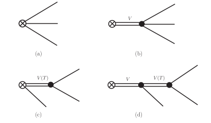
Figure 1: Diagrams contributing to the processes of $e^{+}e^{-}\to K\bar{K}\pi$ at leading order in the $1/N_{C}$ expansion. (a) The Wess-Zumino-Witten anomaly term coming from $\mathcal{L}_{(4)}^{\rm GB}$; (b), (c), and (d) are related to the contributions of vector and tensor resonances.

The chiral anomaly term $\mathcal{L}^{\rm WZW}_{(4)}$ drives Fig. 1 (a), and the electromagnetic current (virtual photon) will couple to the pseudoscalars directly. Fig. 1 (b) is from the $\mathcal{O}_{\rm VPPP}^{j}$. Fig. 1 (c) is related to the $\mathcal{O}_{\rm VJP}^{j}$, $\mathcal{L}^{\rm V}_{(2)}$, $\mathcal{O}_{\rm TJP}^{j}$, and $\mathcal{L}^{\rm T}_{(2)}$ terms, and Fig. 1 (d) is related to the $\mathcal{O}_{\rm VVP}^{j}$, $\mathcal{L}^{\rm V}_{(2)}$, $\mathcal{O}_{\rm TVP}^{j}$, and $\mathcal{L}^{\rm T}_{(2)}$ terms. Compared with those diagrams for the processes of $e^{+}e^{-}\to\pi\pi\pi$, $\pi\pi\eta$ Dai et al. (2013); Qin et al. (2021), the difference is that now we have extra vertexes involving tensors, i.e., the VJP, VVP and VPP vertexes can be replaced by TJP, TVP and TPP vertexes, respectively, See Figs. 1 (c) and (d). The form factors are given as

$$F^{j}_{R}(q^{2},s,t)=F^{j}_{a}+F^{j}_{b}+F^{j}_{c}+F^{j}_{d}.$$ (37)

Here, the subscripts ‘$a,b,c,d$’ correspsond to the Feynman diagrams, and the superscript ‘$j=1,2,3$’ denotes for $K^{+}K^{-}\pi^{0}$, $K^{0}_{S}K^{0}_{L}\pi^{0}$, and $K^{0}_{S}K^{\pm}\pi^{\mp}$ channels, respectively. The form factors for the process of $e^{+}e^{-}\to K^{+}(p_{1})K^{-}(p_{2})\pi^{0}(p_{3})$ are given as

$$F_{a}^{1} = -\frac{N_{C}}{12\pi^{2}F^{3}},$$

$$F_{b}^{1} = \frac{2\sqrt{2}F_{V}}{F^{3}M_{V}}\bigg{\{}\big{[}\frac{1}{M_{\rho}^{2}\!-\!q^{2}}\!+\!\frac{1}{3(M_{\omega}^{2}\!-\!q^{2})}\big{]}GR_{1}(q^{2},s)$$

$$-\frac{2GR_{2}(q^{2},s)}{3(M_{\phi}^{2}\!-\!q^{2})}\bigg{\}},$$

$$F_{c}^{1} = -\frac{2\sqrt{2}G_{V}}{3F^{3}M_{V}}\bigg{\{}\big{[}\frac{1}{M_{\rho}^{2}\!-\!s}\!+\!\frac{3}{M_{\omega}^{2}\!-\!s}\big{]}CR_{1}(q^{2},s,m_{\pi}^{2})$$

$$+\big{[}\frac{CR_{2}(q^{2},t)}{M_{K^{\ast}}^{2}\!-\!t}\!+\!t\leftrightarrow u\big{]}\bigg{\}}$$

$$+\frac{2g_{T}}{F^{3}M_{K_{2}^{\ast}}^{2}}\bigg{\{}\frac{CR^{T}(q^{2},s,t)}{M_{K_{2}^{\ast}}^{2}\!-\!t}\!+\!t\leftrightarrow u\bigg{\}},$$

$$F_{d}^{1} = \frac{2F_{V}G_{V}}{F^{3}}\bigg{\{}\big{[}\frac{2DR(q^{2},s,m_{\pi}^{2})}{(M_{\rho}^{2}\!-\!q^{2})(M_{\omega}^{2}\!-\!s)}\!+\!\frac{1}{3}\big{(}M_{\rho}^{2}\leftrightarrow M_{\omega}^{2}\big{)}\big{]}$$ (38)

$$+\big{[}\frac{1}{M_{\rho}^{2}\!-\!q^{2}}\!+\!\frac{1}{3(M_{\omega}^{2}\!-\!q^{2})}\!-\!\frac{2}{3(M_{\phi}^{2}\!-\!q^{2})}\big{]}$$

$$\times\big{[}\frac{DR(q^{2},m_{K}^{2},t)}{M_{K^{\ast}}^{2}\!-\!t}\!+\!t\leftrightarrow u\big{]}\bigg{\}}$$

$$-\frac{F_{V}g_{T}}{\sqrt{2}F^{3}M_{K_{2}^{\ast}}^{2}}\bigg{\{}\big{[}\frac{1}{M_{\rho}^{2}\!-\!q^{2}}\!+\!\frac{1}{3(M_{\omega}^{2}\!-\!q^{2})}$$

$$+\frac{2}{3(M_{\phi}^{2}\!-\!q^{2})}\big{]}\big{[}\frac{DR^{T}(q^{2},s,t)}{M_{K_{2}^{\ast}}^{2}\!-\!t}\!+\!t\leftrightarrow u\big{]}\bigg{\}},$$

where the functions $GR_{1,2}$, $CR_{1,2}$, $DR$, $CR^{T}$ and $DR^{T}$ are defined in the Appendix C. Similarly, the form factors for $e^{+}e^{-}\to K^{0}_{S}(p_{1})K^{0}_{L}(p_{2})\pi^{0}(p_{3})$ process are derived as

$$F_{a}^{2} = \frac{N_{C}}{12\pi^{2}F^{3}},$$

$$F_{b}^{2} = -\frac{2\sqrt{2}F_{V}}{F^{3}M_{V}}\bigg{\{}\big{[}\frac{1}{M_{\rho}^{2}\!-\!q^{2}}\!-\!\frac{1}{3(M_{\omega}^{2}\!-\!q^{2})}\big{]}GR_{1}(q^{2},s)$$

$$+\frac{2GR_{2}(q^{2},s)}{3(M_{\phi}^{2}\!-\!q^{2})}\bigg{\}},$$

$$F_{c}^{2} = -\frac{2\sqrt{2}G_{V}}{3F^{3}M_{V}}\bigg{\{}\big{[}\frac{1}{M_{\rho}^{2}\!-\!s}\!-\!\frac{3}{M_{\omega}^{2}\!-\!s}\big{]}CR_{1}(q^{2},s,m_{\pi}^{2})$$

$$-2\big{[}\frac{CR_{1}(q^{2},t,m_{K}^{2})}{M^{2}_{K^{\ast}}\!-\!t}\!+\!t\leftrightarrow u\big{]}\bigg{\}},$$

$$F_{d}^{2} = -\frac{2F_{V}G_{V}}{F^{3}}\bigg{\{}\big{[}\frac{2DR(q^{2},s,m_{\pi}^{2})}{(M_{\rho}^{2}\!-\!q^{2})(M_{\omega}^{2}\!-\!s)}\!-\!\frac{1}{3}\big{(}M_{\rho}^{2}\leftrightarrow M_{\omega}^{2}\big{)}\big{]}$$ (39)

$$+\big{[}\frac{1}{M_{\rho}^{2}\!-\!q^{2}}\!-\!\frac{1}{3(M_{\omega}^{2}\!-\!q^{2})}\!+\!\frac{2}{3(M_{\phi}^{2}\!-\!q^{2})}\big{]}$$

$$\times\big{[}\frac{DR(q^{2},t,m_{K}^{2})}{M_{K^{\ast}}^{2}\!-\!t}\!+\!t\leftrightarrow u\big{]}\bigg{\}}$$

$$+\frac{F_{V}g_{T}}{\sqrt{2}F^{3}M_{K_{2}^{\ast}}^{2}}\bigg{\{}\big{[}\frac{1}{M_{\rho}^{2}\!-\!q^{2}}\!-\!\frac{1}{3(M_{\omega}^{2}\!-\!q^{2})}$$

$$-\frac{2}{3(M_{\phi}^{2}\!-\!q^{2})}\big{]}\big{[}\frac{DR^{T}(q^{2},s,t)}{M_{K_{2}^{\ast}}^{2}\!-\!t}\!+\!t\leftrightarrow u\big{]}\bigg{\}}.$$

Notice that the tensor part of Fig. 1 (c) does not have contributions to this process. The form factors of $K^{0}_{S}K^{+}\pi^{-}$ and $K^{0}_{S}K^{-}\pi^{+}$ differ by one overall phase, so we only need to know one of the form factors in these two processes, e.g., $e^{+}e^{-}\to K^{0}_{S}(p_{1})K^{+}(p_{2})\pi^{-}(p_{3})$. One has

$$F_{a}^{3} = 0,$$

$$F_{b}^{3} = \frac{2\sqrt{2}F_{V}}{F^{3}M_{V}}\bigg{\{}\frac{(g_{1}\!+\!2g_{2}\!-\!g_{3})(t\!-\!u)}{M_{\rho}^{2}\!-\!q^{2}}$$

$$-\frac{GR_{1}(q^{2},s)}{3(M_{\omega}^{2}\!-\!q^{2})}\!+\!\frac{2GR_{2}(q^{2},s)}{3(M_{\phi}^{2}\!-\!q^{2})}\bigg{\}},$$

$$F_{c}^{3} = \frac{2\sqrt{2}G_{V}}{3F^{3}M_{V}}\bigg{\{}\frac{CR_{1}(q^{2},s,m_{\pi}^{2})}{M_{\rho}^{2}\!-\!s}\!-\!\frac{2CR_{1}(q^{2},t,m_{K}^{2})}{M^{2}_{K^{\ast}}\!-\!t}$$

$$+\frac{CR_{2}(q^{2},u)}{M^{2}_{K^{\ast}}\!-\!u}\bigg{\}}\!-\!\frac{2g_{T}}{F^{3}}\bigg{\{}\frac{(2c_{1}^{T}\!-\!2c_{2}^{T}\!-\!c_{3}^{T})(t\!-\!u)}{M_{a_{2}}^{2}\!-\!s}$$

$$+\frac{CR^{T}(q^{2},s,u)}{M_{K_{2}^{\ast}}^{2}(M_{K_{2}^{\ast}}^{2}\!-\!u)}\bigg{\}},$$

$$F_{d}^{3} = -\frac{2F_{V}G_{V}}{F^{3}}\bigg{\{}\frac{2DR(q^{2},s,m_{\pi}^{2})}{3(M_{\omega}^{2}\!-\!q^{2})(M_{\rho}^{2}\!-\!s)}$$ (40)

$$-\big{[}\frac{1}{M_{\rho}^{2}\!-\!q^{2}}\!-\!\frac{1}{3(M_{\omega}^{2}\!-\!q^{2})}\!+\!\frac{2}{3(M_{\phi}^{2}\!-\!q^{2})}\big{]}$$

$$\times\frac{DR(q^{2},t,m_{K}^{2})}{M_{K^{\ast}}^{2}\!-\!t}$$

$$+\big{[}\frac{1}{M_{\rho}^{2}\!-\!q^{2}}\!+\!\frac{1}{3(M_{\omega}^{2}\!-\!q^{2})}\!-\!\frac{2}{3(M_{\phi}^{2}\!-\!q^{2})}\big{]}$$

$$\times\frac{DR(q^{2},u,m_{K}^{2})}{M_{K^{\ast}}^{2}\!-\!u}\bigg{\}}$$

$$+\frac{F_{V}g_{T}}{\sqrt{2}F^{3}}\bigg{\{}\frac{2(2d_{1}^{T}\!-\!2d_{2}^{T}\!-\!d_{3}^{T})(t\!-\!u)}{(M_{\rho}^{2}\!-\!q^{2})(M_{a_{2}}^{2}\!-\!s)}$$

$$-\frac{1}{M_{K_{2}^{\ast}}^{2}}\big{[}\big{(}\frac{1}{M_{\rho}^{2}\!-\!q^{2}}\!-\!\frac{1}{3(M_{\omega}^{2}\!-\!q^{2})}\!-\!\frac{2}{3(M_{\phi}^{2}\!-\!q^{2})}\big{)}$$

$$\times\frac{DR^{T}(q^{2},s,t)}{M_{K_{2}^{\ast}}^{2}\!-\!t}$$

$$-\big{(}\frac{1}{M_{\rho}^{2}\!-\!q^{2}}\!+\!\frac{1}{3(M_{\omega}^{2}\!-\!q^{2})}\!+\!\frac{2}{3(M_{\phi}^{2}\!-\!q^{2})}\big{)}$$

$$\times\frac{DR^{T}(q^{2},s,u)}{M_{K_{2}^{\ast}}^{2}\!-\!u}\big{]}\bigg{\}}.$$

Notice that for the processes with final states $K^{0}_{S}(p_{1})K^{\pm}(p_{2})\pi^{\mp}(p_{3})$, Fig. 1 (a) has no contribution, i.e., the Wess-Zumino-Witten anomaly term does not contribute. One needs to add the two cross sections, $\sigma(K^{0}_{S}K^{\pm}\pi^{\mp})=\sigma(K^{0}_{S}K^{+}\pi^{-})+\sigma(K^{0}_{S}K^{-}\pi^{+})=2\sigma(K^{0}_{S}K^{+}\pi^{-})$ to calculate the HVP contributions to the $(g-2)_{\mu}$.

II.4 Constraints on the form factors

There are dozens of unknown couplings coming from the effective Lagrangians that need to be fixed, as shown in the form factors of Eqs. (II.3, II.3, II.3). One can match the Green functions between RChT and QCD in the high energy region to solve this problem Ruiz-Femenia et al. (2003); Dai et al. (2019). Here, we use the constraints obtained by Ref. Dai et al. (2013) that focus on the processes with final states $\pi\pi\pi$ and $\pi\pi\eta$. In that analysis, demanding the two-point Green function of the vector current (with the contributions from the exclusive channels of $\pi\pi\pi$ and $\pi\pi\eta$) to vanish in the energy region $q^{2}\to\infty$ gives

$$g_{1}+2g_{2}-g_{3} = 0,$$

$$g_{2} = \frac{N_{C}M_{V}}{192\sqrt{2}\pi^{2}F_{V}},$$

$$c_{1}-c_{2}+c_{5} = 0,$$

$$c_{1}+c_{2}+8c_{3}-c_{5} = 0,$$

$$c_{1}-c_{2}-c_{5}+2c_{6} = -\frac{N_{C}M_{V}}{96\sqrt{2}\pi^{2}G_{V}},$$

$$d_{3} = -\frac{N_{C}M_{V}^{2}}{192\pi^{2}F_{V}G_{V}}.$$ (41)

Moreover, if we adopt the same scheme as Ref. Dai et al. (2013) to get short distance constraints in the process of $e^{+}e^{-}\to K\bar{K}\pi$, the matching procedure gives two extra constraints for the tensor couplings,

$$2c_{1}^{T}-2c_{2}^{T}-c_{3}^{T} = 0,$$

$$2d_{1}^{T}-2d_{2}^{T}-d_{3}^{T} = 0.$$

Unfortunately, the widths of $\Gamma(a_{2}^{\pm}\to\pi^{\pm}\gamma)$, $\Gamma(K_{2}^{\ast}\to K^{\ast}\pi)$, $\Gamma(K_{2}^{\ast}\to\rho(\omega)K)$, and $\Gamma(K_{2}^{\ast\pm}\to K^{\pm}\gamma)$ would vanish if we apply these short distance constraints, which is incompatible with the experimental data Workman et al. (2022). See discussions in the next sections. This conflict may be due to the lack of insight into the tensor current. Therefore, we leave $2c_{1}^{T}-2c_{2}^{T}-c_{3}^{T}$ and $2d_{1}^{T}-2d_{2}^{T}-d_{3}^{T}$ free, but determine them with the fit to the experiment data for the tensor resonances. In addition, $g_{4}$ and $c_{4}$ have been studied in the analysis of $\tau\to KK\pi\nu_{\tau}$ Dumm et al. (2010a), which can be a guide to the present analysis. We also take the short distance constraints obtained in other analyses, such as those from the two-pion vector form factor and from the study of matching the three-point $\langle VVP\rangle$ Green functions between QCD and RChT Ruiz-Femenia et al. (2003),

$$F_{V}G_{V}=F^{2},~{}~{}~{}d_{1}+8d_{2}-d_{3}=\frac{F^{2}}{8F_{V}^{2}}.$$ (42)

With these constraints, we have reduced the unknown coupling constants, and only a few of them are left, i.e., $F_{V}$, $g_{4}$, $c_{4}$, $2g_{4}+g_{5}$, $g_{T}$, $c_{3}^{T}$, $d_{3}^{T}$, $2c_{1}^{T}-2c_{2}^{T}-c_{3}^{T}$, and $2d_{1}^{T}-2d_{2}^{T}-d_{3}^{T}$.

The interaction Lagrangians discussed above are only for the lightest vector and tensor mesons, which dominate the interactions around 1 GeV. However, the heavier states appear in the higher energy region and would contribute, too. In order to account for the excited resonance effects up to the energy region that we studied, $E_{\rm cm}\sim 2.3$ GeV, we adopt the same strategy as done in Refs. Dai et al. (2013); Qin et al. (2021); Wang et al. (2023) to deal with the heavier states. Here, we include two multiplets of the vector resonances ($V^{\prime}_{\mu\nu}$ and $V_{\mu\nu}^{\prime\prime}$) and one multiplet of tensor resonances ($T^{\prime}_{\mu\nu}$), since the second excited tensor resonances lie above the energy region we focus on. These heavier multiplets are included by extension of the Breit-Wigner propagator Dai et al. (2013)

$$\frac{1}{M_{R}^{2}-x}\to\frac{1}{M_{R}^{2}-x}+\frac{\beta^{R^{\prime}}_{j}}{M_{R^{\prime}}^{2}-x}+\frac{\beta^{R^{\prime\prime}}_{j}}{M_{R^{\prime\prime}}^{2}-x},$$ (43)

where $R=V,T$ and $\beta^{T^{\prime\prime}}_{j}=0$. The subscript ‘$j=1,2,3$’ represents the $K^{+}K^{-}\pi^{0}$, $K^{0}_{S}K^{0}_{L}\pi^{0}$, and $K^{0}_{S}K^{\pm}\pi^{\mp}$ channels, respectively. Indeed, assuming that one writes down these heavier fields explicitly in the chiral effective Lagrangians, the Feynman diagrams will have the identical topologies as those given in Fig. 1, and the form factors will have similar formalism with only some energy functions absorbed into the parameters of $\beta_{j}^{R^{\prime},R^{\prime\prime}}$. For convenience, we collect the lightest vector and tensor resonances $R$ and their heavier partners $R^{\prime}$, $R^{\prime\prime}$ that are used in the present analysis,

$$R\! = \!\big{\{}\rho(770),\omega(782),\phi(1020),K^{\ast}(892),$$

$$~{}~{}a_{2}(1320),K_{2}^{\ast}(1430)\big{\}},$$

$$R^{\prime}\! = \!\big{\{}\rho(1450),\omega(1420),\phi(1680),K^{\ast}(1410),$$

$$~{}~{}a_{2}(1700),K_{2}^{\ast}(1980)\big{\}},$$

$$R^{\prime\prime}\! = \!\big{\{}\rho(1700),\omega(1650),\phi(2170),K^{\ast}(1680)\big{\}}.$$

In addition, one would notice that the propagator in the form factors of Eq. (37) are real, while in the real world, the resonances have unignorable widths. Also, the energy-dependent widths can give a better description of the data. These are fulfilled by applying the well-known Breit-Wigner propagators

$$\frac{1}{M_{R}^{2}-x}\to\frac{1}{M_{R}^{2}-x-iM_{R}\Gamma_{R}(x)},$$ (44)

where the widths of $\rho(770)$ and $K^{\ast}(892)$ and their corresponding excited states are taken in the energy-dependent form. See Appendix D. For the other resonances, constant widths from PDG Workman et al. (2022) are adopted.

Besides, in the high energy region, the form factors will be divergent, as the terms of $m_{K}^{2}$ (multiplied together with the momentum) have significant contributions, while it is ignored in the chiral limit when the high energy constraints are obtained. To fix this problem, we follow the method applied in Ref. Wang et al. (2023) and implement a regulator $f(q^{2})={\rm exp}\left\{-q^{6}/\Lambda^{6}\right\}$ Yang et al. (2023) in the form factors, where the cut off is chosen as $\Lambda=2.5$ GeV. Here is a point to be emphasized this function works like a step function and will have little contribution in the energy region below 2.0 GeV.

In order to take more constraints from the experiment, the correlated decay processes of the vector meson, $K^{\ast}$, and tensor mesons, $a_{2}$ and $K_{2}^{\ast}$, are also calculated, that is, $K^{\ast}\to PP/P\gamma$, $a_{2}\to PP/P\gamma$ and $K_{2}^{\ast}\to PP/VP/P\gamma$, where $P$ is the pseudoscalar. Here, one has $K^{\ast}=K^{\ast}(892)$, $a_{2}=a_{2}(1320)$ and $K_{2}^{\ast}=K_{2}^{\ast}(1430)$. The complete expressions for these decay widths are collected in Appendix E. What is more, the mixing angle $\theta_{P}$ will affect the decay widths of $a_{2}\to\eta\pi$, $\eta^{\prime}\pi$, and it should also be determined by the fit. Also, there need three normalization factors, $N_{1},N_{2},N_{3}$, which are multiplied by the differential cross section to fit the events distribution of the invariant mass spectra. Finally, the processes of $e^{+}e^{-}\to K\bar{K}\pi$ and the correlated decays of the resonances are studied within RChT. After taking the short distance constraints, there are still some parameters left to be fixed by the experimental data, i.e., $F_{V}$, $g_{4}$, $c_{4}$, $2g_{4}+g_{5}$, $g_{T}$, $c_{3}^{T}$, $d_{3}^{T}$, $2c_{1}^{T}-2c_{2}^{T}-c_{3}^{T}$, $2d_{1}^{T}-2d_{2}^{T}-d_{3}^{T}$, $\beta^{V^{\prime}}_{j}$, $\beta^{V^{\prime\prime}}_{j}$, $\beta^{T^{\prime}}_{j}$, and the mixing angle $\theta_{P}$ of $\eta-\eta^{\prime}$. In addition, the masses and widths of the heavier resonances are restricted by PDG Workman et al. (2022).

III Numerical results

To reach a comprehensive analysis and obtain reliable form factors, we fit our amplitudes to all the datasets of the cross sections, two-body invariant mass spectra, and decay widths of vectors and tensors. The cross sections of the processes of electron-positron annihilation into $K\bar{K}\pi$ ($K^{+}K^{-}\pi^{0}$, $K^{0}_{S}K^{0}_{L}\pi^{0}$ and $K^{0}_{S}K^{\pm}\pi^{\mp}$) are measured by Refs. Mane et al. (1982); Bisello et al. (1991); Aubert et al. (2008); Solodov et al. (2016); Lees et al. (2017); Achasov et al. (2018); Semenov et al. (2019); Achasov et al. (2020); Ablikim et al. (2022, 2024). Following the strategy applied in Refs. Qin et al. (2021); Wang et al. (2023), we only fit the data sets after the year 2000, and the ones before 2000 are only plotted for the reader’s convenience due to their poor statistics. As is well known, the angular distribution data sets are helpful for constraining the amplitude Dai and Pennington (2014a, b). Here, there are three kinds of datasets for the invariant mass spectra Achasov et al. (2020, 2018), ($M_{K^{\pm}\pi^{0}}$, $M_{K_{S/L}^{0}\pi^{0}}$ and $M_{K_{S}^{0}K_{L}^{0}}$) for the relevant processes of $e^{+}e^{-}\to K\bar{K}\pi$, which are included in our fit to refine the present analysis, as $t,u$ are functions of the Mandelstam variable $s$ in the $s$-channel and the scattering angle $\theta_{s}$. Most of these invariant mass spectra are in the energy region of [$1.5-1.75$] GeV, which can help check the reliability of our model, where the generalizing propagators are applied to include the contributions of the heavier resonances. We summarize all the datasets in Table 1.

	$K^{+}K^{-}\pi^{0}$	$K^{0}_{S}K^{0}_{L}\pi^{0}$	$K^{0}_{S}K^{\pm}\pi^{\mp}$
DM1	$-$	$-$	Mane et al. (1982)
DM2	Bisello et al. (1991)	$-$	Bisello et al. (1991)
BABAR	Aubert et al. (2008)	Lees et al. (2017)	Aubert et al. (2008)
SND	Achasov et al. (2020)	Achasov et al. (2018)	$-$
CMD-3	Solodov et al. (2016)	Semenov et al. (2019)	$-$
BESIII	Ablikim et al. (2022)	Ablikim et al. (2024)	$-$

Table 1: The datasets of the process of $e^{+}e^{-}\to K\bar{K}\pi$ adopted for the present analysis.

The fitting parameters are listed in Table 2.

$\rm Parameters$	$\rm This~{}analysis$	$\rm Ref$. Dai et al. (2013)	$\rm Ref$. Qin et al. (2021)	$\rm Ref$. Wang et al. (2023)	$\rm PDG$ Workman et al. (2022)
$F_{V}(\rm GeV)$	$0.1469\pm 0.0007$	$0.148\pm 0.001$	$0.142\pm 0.001$	$0.138\pm 0.001$
$g_{4}$	$-0.0331\pm 0.0012$	$-$	$-$	$-$
$c_{4}$	$-0.0013\pm 0.0001$	$-$	$-$	$-$
$2g_{4}+g_{5}$	$-0.0166\pm 0.0041$	$-0.493\pm 0.003$	$-0.492\pm 0.002$	$-$
$g_{T}(\rm GeV)$	$0.0233\pm 0.0004$	$-$	$-$	$-$
$c_{3}^{T}$	$0.2809\pm 0.0348$	$-$	$-$	$-$
$d_{3}^{T}$	$-0.5893\pm 0.4253$	$-$	$-$	$-$
$2c_{1}^{T}-2c_{2}^{T}-c_{3}^{T}$	$0.0214\pm 0.0012$	$-$	$-$	$-$
$2d_{1}^{T}-2d_{2}^{T}-d_{3}^{T}$	$0.5535\pm 0.0133$	$-$	$-$	$-$
$\theta_{P}(^{\circ})$	$-20.50\pm 0.26$	$-21.37\pm 0.26$	$-19.61\pm 0.10$	$-20.50\pm 0.30$
$\beta^{V^{\prime}}_{1}$	$-0.3154\pm 0.0032$	$-$	$-$	$-$
$\beta^{V^{\prime\prime}}_{1}$	$-0.0345\pm 0.0021$	$-$	$-$	$-$
$\beta^{V^{\prime}}_{2}$	$-0.4447\pm 0.0018$	$-$	$-$	$-$
$\beta^{V^{\prime\prime}}_{2}$	$0.0205\pm 0.0030$	$-$	$-$	$-$
$\beta^{V^{\prime}}_{3}$	$-0.4395\pm 0.0022$	$-$	$-$	$-$
$\beta^{V^{\prime\prime}}_{3}$	$0.0332\pm 0.0083$	$-$	$-$	$-$
$M_{\rho^{\prime}}(\rm GeV)$	$1.5500\pm 0.0005$	$1.550\pm 0.012$	$1.519\pm 0.002$	$1.519\pm 0.001$	$1.465\pm 0.025$
$\Gamma_{\rho^{\prime}}(\rm GeV)$	$0.2400\pm 0.0004$	$0.238\pm 0.018$	$0.340\pm 0.001$	$0.381\pm 0.003$	$0.400\pm 0.060$
$M_{\omega^{\prime}}(\rm GeV)$	$1.4253\pm 0.0043$	$1.249\pm 0.003$	$1.253\pm 0.003$	$1.250\pm 0.003$	$1.410\pm 0.060$
$\Gamma_{\omega^{\prime}}(\rm GeV)$	$0.1612\pm 0.0073$	$0.307\pm 0.007$	$0.310\pm 0.003$	$0.290\pm 0.002$	$0.290\pm 0.190$
$M_{\phi^{\prime}}(\rm GeV)$	$1.6540\pm 0.0014$	$1.641\pm 0.005$	$1.640\pm 0.003$	$1.656\pm 0.003$	$1.680\pm 0.020$
$\Gamma_{\phi^{\prime}}(\rm GeV)$	$0.1680\pm 0.0011$	$0.086\pm 0.007$	$0.090\pm 0.002$	$0.136\pm 0.001$	$0.150\pm 0.050$
$M_{K^{\ast^{\prime}}}(\rm GeV)$	$1.4500\pm 0.0060$	$-$	$-$	$-$	$1.414\pm 0.015$
$\Gamma_{K^{\ast^{\prime}}}(\rm GeV)$	$0.2500\pm 0.0056$	$-$	$-$	$-$	$0.232\pm 0.021$
$M_{\rho^{\prime\prime}}(\rm GeV)$	$1.7600\pm 0.0019$	$1.794\pm 0.012$	$1.720\pm 0.001$	$1.720\pm 0.001$	$1.720\pm 0.020$
$\Gamma_{\rho^{\prime\prime}}(\rm GeV)$	$0.3500\pm 0.0228$	$0.297\pm 0.033$	$0.150\pm 0.005$	$0.250\pm 0.001$	$0.250\pm 0.100$
$M_{\omega^{\prime\prime}}(\rm GeV)$	$1.6303\pm 0.0555$	$1.700\pm 0.011$	$1.725\pm 0.010$	$1.725\pm 0.002$	$1.670\pm 0.030$
$\Gamma_{\omega^{\prime\prime}}(\rm GeV)$	$0.3997\pm 0.0868$	$0.400\pm 0.013$	$0.400\pm 0.003$	$0.400\pm 0.001$	$0.315\pm 0.035$
$M_{\phi^{\prime\prime}}(\rm GeV)$	$2.1741\pm 0.0051$	$2.086\pm 0.022$	$2.126\pm 0.025$	$2.160\pm 0.001$	$2.162\pm 0.007$
$\Gamma_{\phi^{\prime\prime}}(\rm GeV)$	$0.1075\pm 0.0072$	$0.108\pm 0.017$	$0.100\pm 0.014$	$0.105\pm 0.010$	$0.100^{+0.031}_{-0.023}$
$M_{K^{\ast^{\prime\prime}}}(\rm GeV)$	$1.7500\pm 0.0590$	$-$	$-$	$-$	$1.718\pm 0.018$
$\Gamma_{K^{\ast^{\prime\prime}}}(\rm GeV)$	$0.4300\pm 0.0612$	$-$	$-$	$-$	$0.322\pm 0.110$

Table 2: Fitted parameters of our solution, compared with Fit 4 in Ref. Dai et al. (2013), Fit II in Ref. Qin et al. (2021), Fit B in Ref. Wang et al. (2023), and PDG Workman et al. (2022). The uncertainties of the parameters are taken from MINUIT James and Roos (1975).

In practice, it is found that one can set $\beta^{T^{\prime}}_{j}=\beta^{V^{\prime}}_{j}$, and the results are almost as good as what is obtained by setting them free. In the present analysis, the magnitude of the parameter $2g_{4}+g_{5}$ is much smaller than what is obtained from the analyses on $e^{+}e^{-}\to\pi\pi\pi$, $\pi\pi\eta$ Dai et al. (2013); Qin et al. (2021). The reason is that in the $\pi\pi\pi$ and $\pi\pi\eta$ cases, the $2g_{4}+g_{5}$ is multiplied with the mass term $m_{\pi}^{2}$, while we have $(2g_{4}+g_{5})m_{K}^{2}$ here. See Eq. (52). One would need a smaller $2g_{4}+g_{5}$ multiplying $m_{K}^{2}$ to have similar contributions with that of $(2g_{4}+g_{5})m_{\pi}^{2}$. Parameters obtained in other works Dai et al. (2013); Qin et al. (2021); Wang et al. (2023) and those from PDG are also listed for comparison. A consistent set of parameters is obtained in this work, considering the corresponding uncertainties. The masses and widths of the ground states of vectors and tensors that are used in this analysis are fixed by PDG Workman et al. (2022).

The decay widths predicted by our model are given in Table 3. In an overall view, they are compatible with those of PDG.

$\rm Width$	$\rm Unit~{}(GeV)$	$\rm This~{}analysis$	$\rm PDG$ Workman et al. (2022)
$\Gamma(K^{\ast}\!\to\!K\pi)$	$10^{-2}$	$4.549\pm 0.154$	$4.935\pm 0.065$
$\Gamma(K^{\ast 0}\!\to\!K^{0}\gamma)$	$10^{-4}$	$1.055\pm 0.014$	$1.164\pm 0.100$
$\Gamma(K^{\ast\pm}\!\to\!K^{\pm}\gamma)$	$10^{-5}$	$3.450\pm 0.316$	$5.040\pm 0.470$
$\Gamma(a_{2}\!\to\!\eta\pi)$	$10^{-2}$	$2.198\pm 0.089$	$1.552\pm 0.147$
$\Gamma(a_{2}\!\to\!K\bar{K})$	$10^{-3}$	$5.680\pm 0.232$	$5.243\pm 0.890$
$\Gamma(a_{2}\!\to\!\eta^{\prime}\pi)$	$10^{-4}$	$4.515\pm 0.216$	$5.885\pm 1.002$
$\Gamma(a_{2}^{\pm}\!\to\!\pi^{\pm}\gamma)$	$10^{-4}$	$4.458\pm 0.239$	$3.114\pm 0.323$
$\Gamma(K_{2}^{\ast}\!\to\!K\pi)$	$10^{-2}$	$4.304\pm 0.176$	$5.215\pm 0.217$
$\Gamma(K_{2}^{\ast}\!\to\!K^{\ast}\pi)$	$10^{-2}$	$1.365\pm 0.133$	$2.581\pm 0.180$
$\Gamma(K_{2}^{\ast}\!\to\!\rho K)$	$10^{-3}$	$4.899\pm 0.476$	$9.092\pm 0.891$
$\Gamma(K_{2}^{\ast}\!\to\!\omega K)$	$10^{-3}$	$1.424\pm 0.138$	$3.031\pm 0.842$
$\Gamma(K_{2}^{\ast\pm}\!\to\!K^{\pm}\gamma)$	$10^{-4}$	$2.476\pm 0.164$	$2.400\pm 0.503$

Table 3: Fitting results for the decay widths and PDG data are for 2022.

Indeed, all the other decay widths are in good agreement with the data, except for the decay widths of $K_{2}^{\ast}\to\rho K$, $\omega K$, and $K^{\ast}\pi$, which deviates from the PDG about fifty percent. The reason may be that in these processes, the final states include a vector meson, while in all other decays, the final states contain only pseudoscalars and/or photons. The vector meson will decay into the lighter mesons and/or photons, and one lacks the dynamical description of the final state interactions (FSI) for these subsequent processes. Also, they are all for the tensors, which have been inadequately studied until now. Nevertheless, the fit to the decay widths gives more constraints on the coupling constants and helps to extract the form factors more reliably. We apply the Bootstrap method Efron (1979) to obtain the uncertainties of our solution, which are calculated by varying the experimental data points within their errors and multiplying a normal distribution function. In contrast, the errors from MINUIT James and Roos (1975) are tiny and ignorable.

An overall sound fit to the cross sections and invariant mass spectra are shown in Fig. 2.

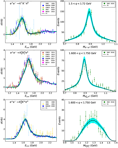
Figure 2: Fit to the cross sections and invariant mass spectra. The left three graphs are for the cross sections of $e^{+}e^{-}\to K^{+}K^{-}\pi^{0}$, $K_{S}^{0}K_{L}^{0}\pi^{0}$ and $K_{S}^{0}K^{\pm}\pi^{\mp}$, where the data are from DM1 Mane et al. (1982), DM2 Bisello et al. (1991), BABAR Aubert et al. (2008); Lees et al. (2017), SND Achasov et al. (2018, 2020), CMD-3 Solodov et al. (2016); Semenov et al. (2019) and BESIII Ablikim et al. (2022, 2024). The right three graphs are for the invariant mass spectra of $M_{K^{\pm}\pi^{0}}$, $M_{K_{S/L}^{0}\pi^{0}}$ and $M_{K_{S}^{0}K_{L}^{0}}$ from the $K^{+}K^{-}\pi^{0}$ and $K_{S}^{0}K_{L}^{0}\pi^{0}$ processes measured by SND Achasov et al. (2020, 2018).

As can be found, ours fits the data well. There is a broad peak in the energy region of $E_{\rm cm}\in[1.5-1.7]$ GeV for the cross sections. It may be caused by the complicated interaction involving the excited resonances, $V^{\prime(\prime\prime)}$, except for the $\phi(2170)$. The solution in this energy region is strongly constrained by the invariant mass spectra as given in the graphs in the right column of Fig. 2. Indeed, our solution fits the total cross sections better than that of the invariant mass spectra. In the right side graph of the second row of Fig. 2, the ‘peak’ looks like it has been shifted a bit to the left side. This may be caused by a lack of accurate methods to describe the final state interactions between the pion and kaon, of which we apply an energy-dependent width for $K^{\ast}(892)$ to restore it partly. See Eq. (D). Also, the ‘peak’ in the right side graph of the third row looks like it is shifted a bit to the right side. This may be caused by a lack of a precise model to describe $K\bar{K}$ FSI. All the experimental data sets of invariant mass spectra are from SND Achasov et al. (2020, 2018), and the statistics are not high. Nevertheless, a combination fit to the invariant mass spectra and the rich data sets of the cross sections imposes a strong constraint on the parameters of our solution, which helps to give a reliable estimation of the $K\bar{K}\pi$ contribution to HVP.

IV The muon anomalous magnetic moment

With the cross sections obtained above, one can predict their contributions to the leading order (LO) HVP of the muon anomalous magnetic moment. One has Brodsky and De Rafael (1968); Lautrup and De Rafael (1968)

$$a_{\mu}^{\rm HVP,LO}=\frac{\alpha_{e}^{2}(0)}{3\pi^{2}}\int_{s_{\rm th}}^{\infty}ds\frac{\hat{K}(s)}{s}R_{\rm h}(s),$$ (45)

where $\alpha_{e}(0)=e^{2}/(4\pi)$ is the electromagnetic fine-structure constant and the kernel function $\hat{K}(s)$ can be found in Ref. Aoyama et al. (2020). The hadronic $R$-ratio is derived as

$$R_{\rm h}(s)=\frac{3s}{4\pi\alpha_{e}^{2}(s)}\sigma\bigg{(}e^{+}e^{-}\to{\rm hadrons}\bigg{)}.$$ (46)

Here, the $\alpha_{e}(s)$ can be found in Ref. Wang et al. (2023)

$$\alpha_{e}(s)=\frac{\alpha_{e}(0)}{1-\Delta\alpha(s)}\,,~{}~{}~{}\Delta\alpha(s)=\Pi^{\prime}_{\gamma}(0)-\Pi^{\prime}_{\gamma}(s)\,,$$

where $\Pi_{\gamma}(s)$ is the vacuum polarization operator. The total cross sections of $e^{+}e^{-}\to K\bar{K}\pi$ include three kinds of final states as Keshavarzi et al. (2018)

$$\sigma(K\bar{K}\pi)\!=\!\sigma(K^{+}K^{-}\pi^{0})\!+\!\sigma(K_{S}^{0}K_{L}^{0}\pi^{0})\!+\!2\sigma(K_{S}^{0}K^{\pm}\pi^{\mp})\,.$$

The prediction of the $(g-2)_{\mu}$ from $e^{+}e^{-}\to K\bar{K}\pi$ are given in Table 4 and their contributions to HVP from other works Keshavarzi et al. (2018); Davier et al. (2020) are listed for comparison.

$a_{\mu}\times 10^{-10}$	$\rm This~{}analysis$	$\rm KNT18$ Keshavarzi et al. (2018)	$\rm DHMZ19$ Davier et al. (2020)
$a_{\mu}^{K\bar{K}\pi}[1.260\leq q\leq 1.937~{}{\rm GeV}]$	$2.62\pm 0.07$	$2.71\pm 0.12$	$-$
$a_{\mu}^{K\bar{K}\pi}[{\rm th.}\leq q\leq 1.8~{}{\rm GeV}]$	$2.30\pm 0.06$	$2.44\pm 0.11$	$2.45\pm 0.13$
$a_{\mu}^{K\bar{K}\pi}[{\rm th.}\leq q\leq 2~{}{\rm GeV}]$	$2.73\pm 0.07$	$2.80\pm 0.12$	$-$
$a_{\mu}^{K\bar{K}\pi}[{\rm th.}\leq q\leq 2.3~{}{\rm GeV}]$	$3.07\pm 0.07$	$-$	$-$

Table 4: Our predictions of the contributions of the muon anomalous magnetic moment from $e^{+}e^{-}\to K\bar{K}\pi$. We also list the results of other works to give a comparison Keshavarzi et al. (2018); Davier et al. (2020). The ${\rm th.}$ denotes the threshold of $K\bar{K}\pi$.

It is found that our estimation of the contributions of $K\bar{K}\pi$ is in good agreement with those gained by data-driven method Keshavarzi et al. (2018); Davier et al. (2020) below 2 GeV. Moreover, our calculation of $K\bar{K}\pi$ channel contribution is up to 2.3 GeV within RChT, with the corresponding $a_{\mu}$ as $(3.07\pm 0.07)\times 10^{-10}$. For reader’s convenience, we also give an estimation of the $a_{\mu}$ from threshold up to 1.8 GeV, as $(2.30\pm 0.06)\times 10^{-10}$. This is a bit smaller than those of Refs. Keshavarzi et al. (2018); Davier et al. (2020). It would be rather helpful if the experiments could perform measurements about the cross sections and angular distributions with higher statistics. Studies on other processes with multi-pseudoscalar, e.g., $e^{+}e^{-}\to 4\pi$ would refine the estimation on the theoretical prediction of HVP and give an answer to the discrepancy of $(g-2)_{\mu}$.

V Conclusion and summary

In this work, we systematically studied the processes of $e^{+}e^{-}\to K^{+}K^{-}\pi^{0}$, $K_{S}^{0}K_{L}^{0}\pi^{0}$, and $K_{S}^{0}K^{\pm}\pi^{\mp}$ within the framework of resonance chiral theory. The experimental data of scattering cross sections, invariant mass spectra, and decay widths of the vectors and tensors are fitted to fix the unknown parameters. A high-quality solution is obtained. With it, we predict the LO HVP contributions to the muon anomalous magnetic moment, $a_{\mu}^{K\bar{K}\pi}=(3.07\pm 0.07)\times 10^{-10}$, from threshold up to $E_{\rm cm}=$2.3 GeV, or for convenience of the reader, $a_{\mu}^{K\bar{K}\pi}=(2.30\pm 0.06)\times 10^{-10}$, from threshold up to $E_{\rm cm}=1.8$ GeV. Further theoretical studies and experimental measurements on the electron-positron annihilation into hadrons are needed to improve the prediction on $(g-2)_{\mu}$ from the Standard Model.

Appendix A Feynman propagator and polarization of tensor

The Feynman propagator of the tensor is defined as Bellucci et al. (1994); Ecker and Zauner (2007)

$$G_{\mu\nu,\rho\sigma}^{T}(x) = \int\frac{d^{4}k}{(2\pi)^{4}}\frac{iP_{\mu\nu,\rho\sigma}(k)}{M_{T}^{2}-k^{2}-i\epsilon}{\rm e}^{-ikx},$$ (47)

where $k$ is the momentum, and one has

$$P_{\mu\nu,\rho\sigma}(k) = \frac{1}{2}(P_{\mu\rho}P_{\nu\sigma}+P_{\nu\rho}P_{\mu\sigma})-\frac{1}{3}P_{\mu\nu}P_{\rho\sigma}\,,$$

$$P_{\mu\nu} = g_{\mu\nu}-\frac{k_{\mu}k_{\nu}}{M_{T}^{2}}\,.$$

The tensor field operator $T_{\mu\nu}$ acting on the state of a spin-2 particle is expressed in terms of the polarization tensor $\varepsilon_{\mu\nu}(k,\lambda)$ Ecker and Zauner (2007):

$$\langle 0|T_{\mu\nu}(0)|T(k;\lambda)\rangle=\varepsilon_{\mu\nu}(k;\lambda).$$ (48)

with $\lambda$ the polarization. The sum over all polarizations gives

$$\sum_{\lambda}\varepsilon_{\mu\nu}(k;\lambda)\varepsilon_{\rho\sigma}(k;\lambda)^{\ast}=P_{\mu\nu,\rho\sigma}(k).$$

Appendix B Effective Lagrangians with tensor

As is known, the effective Lagrangians should satisfy discrete symmetries Ecker et al. (1989a); Bijnens et al. (1999); Fettes et al. (2000). The properties of chiral operators transforming under the parity ($P$), charge conjugation ($C$), and hermiticity (h.c.) are given in Table 5.

$\rm Operator$	$\rm Dim$	$P$	$C$	$\rm h.c.$
$u_{\mu}$	$1$	$-u^{\mu}$	$(u_{\mu})^{T}$	$u_{\mu}$
$h_{\mu\nu}$	$2$	$-h^{\mu\nu}$	$(h_{\mu\nu})^{T}$	$h_{\mu\nu}$
$\chi_{\pm}$	$2$	$\pm\chi_{\pm}$	$(\chi_{\pm})^{T}$	$\pm\chi_{\pm}$
$f^{\mu\nu}_{\pm}$	$2$	$\pm f_{\pm\mu\nu}$	$\mp(f^{\mu\nu}_{\pm})^{T}$	$f^{\mu\nu}_{\pm}$
$V_{\mu\nu}$	$0$	$V^{\mu\nu}$	$-(V_{\mu\nu})^{T}$	$V_{\mu\nu}$
$T_{\mu\nu}$	$0$	$T^{\mu\nu}$	$(T_{\mu\nu})^{T}$	$T_{\mu\nu}$
$\varepsilon_{\mu\nu\rho\sigma}$	$0$	$-\varepsilon^{\mu\nu\rho\sigma}$	$\varepsilon_{\mu\nu\rho\sigma}$	$\varepsilon_{\mu\nu\rho\sigma}$

Table 5: The chiral dimension (Dim), $P$, $C$ and h.c. transformation properties of operators for constructing chiral Lagrangians.

Following it, we construct the Lagrangians about TJP and TVP terms mentioned in the above sections. We use the following constraints to select the linearly independent terms among all the possible combinations of the operators Ruiz-Femenia et al. (2003):

(i) Equations of motion (EOM) Bijnens et al. (1999).

$$\nabla_{\mu}u^{\mu}=\frac{i}{2}\left(\chi_{-}-\frac{1}{n_{f}}\langle\chi_{-}\rangle\right),$$ (49)

with $n_{f}$ the number of light flavors ($n_{f}=3$ in our case). With this equation, $\nabla_{\mu}u^{\mu}$ will not appear in the chiral effective Lagrangians as it can be replaced by $\chi_{-}$.

(ii) Total derivative Fearing and Scherer (1996); Ebertshauser et al. (2002).

$$\langle\nabla_{\mu}\left(ABC\cdots\right)\rangle = \langle\left(\nabla_{\mu}A\right)BC\cdots\rangle+\langle A\left(\nabla_{\mu}B\right)C\cdots\rangle$$ (50)

$$+~{}\langle AB\left(\nabla_{\mu}C\right)\cdots\rangle+\cdots,$$

where $\nabla_{\mu}$ is the covariant derivative, and $A,B,C,\cdots$ represent the operators. The total derivative would lead to a vanished action integrated from the Lagrangians with a total derivative. Correspondingly, one should reduce one of the terms on the right side of the equal sign as they are not independent.

(iii) Schouten identity.

$$g_{\alpha\lambda}\varepsilon_{\mu\nu\rho\sigma}+g_{\alpha\mu}\varepsilon_{\nu\rho\sigma\lambda}+g_{\alpha\nu}\varepsilon_{\rho\sigma\lambda\mu}$$

$$+g_{\alpha\rho}\varepsilon_{\sigma\lambda\mu\nu}+g_{\alpha\sigma}\varepsilon_{\lambda\mu\nu\rho}=0.$$ (51)

With these constraints, we are able to pick out the independent effective Lagrangians, and finally, the TJP and TVP interaction Lagrangians are given in Eqs. (32, 33).

Appendix C Notations for the form factors

The notations of the form factors employed in the text are specified below:

$$GR_{1}(q^{2},s) = (g_{1}+2g_{2}-g_{3})(q^{2}+s-4m_{K}^{2}-m_{\pi}^{2})+4(2g_{4}+g_{5})m_{K}^{2}-4g_{2}(q^{2}-2m_{K}^{2}-m_{\pi}^{2})-4g_{4}(m_{K}^{2}-m_{\pi}^{2}),$$

$$GR_{2}(q^{2},s) = (g_{1}+2g_{2}-g_{3})(q^{2}-s-m_{\pi}^{2})+2(2g_{4}+g_{5})m_{\pi}^{2}-2g_{2}(q^{2}-2m_{K}^{2}-m_{\pi}^{2})+4g_{4}(m_{K}^{2}-m_{\pi}^{2}),$$

$$CR_{1}(q^{2},x,m^{2}) = (c_{1}-c_{2}+c_{5})q^{2}-(c_{1}-c_{2}-c_{5}+2c_{6})x+(c_{1}+c_{2}+8c_{3}-c_{5})m^{2},$$

$$CR_{2}(q^{2},x) = (c_{1}-c_{2}+c_{5})q^{2}-(c_{1}-c_{2}-c_{5}+2c_{6})x+(c_{1}+c_{2}+8c_{3}-c_{5})m_{K}^{2}+24c_{4}(m_{K}^{2}-m_{\pi}^{2}),$$

$$DR(q^{2},x,m^{2}) = (d_{1}+8d_{2}-d_{3})m^{2}+d_{3}(q^{2}+x),$$

$$CR^{T}(q^{2},s,x) = (2c_{1}^{T}-2c_{2}^{T}-c_{3}^{T})\Big{[}M_{K_{2}^{\ast}}^{2}(q^{2}-2s-x+3m_{K}^{2})+(q^{2}-x-m_{K}^{2})(m_{K}^{2}-m_{\pi}^{2})\Big{]}$$

$$+2c_{3}^{T}(M_{K_{2}^{\ast}}^{2}-x)(m_{K}^{2}-m_{\pi}^{2}),$$

$$DR^{T}(q^{2},s,x) = (2d_{1}^{T}-2d_{2}^{T}-d_{3}^{T})\Big{[}M_{K_{2}^{\ast}}^{2}(q^{2}-2s-x+3m_{K}^{2})+(q^{2}-x-m_{K}^{2})(m_{K}^{2}-m_{\pi}^{2})\Big{]}$$ (52)

$$+2d_{3}^{T}(M_{K_{2}^{\ast}}^{2}-x)(m_{K}^{2}-m_{\pi}^{2}).$$

Appendix D The energy-dependent widths of the vector resonances

The energy-dependent widths of the vector resonances taken from Refs. Dai et al. (2013); Dumm et al. (2010b); Jamin et al. (2006)

$$\Gamma_{\rho}(s) = \frac{M_{\rho}s}{96\pi F^{2}}\Big{\{}\sigma_{\pi}^{3}(s)\theta(s-4m_{\pi}^{2})$$

$$+\frac{1}{2}\sigma_{K}^{3}(s)\theta(s-4m_{K}^{2})\Big{\}},$$

$$\Gamma_{\rho^{\prime}}(s) = \Gamma_{\rho^{\prime}}\frac{\sqrt{s}}{M_{\rho^{\prime}}}\Big{\{}\frac{\sigma_{\pi}^{3}(s)}{\sigma_{\pi}^{3}(M_{\rho^{\prime}}^{2})}\Big{\}}\theta(s-4m_{\pi}^{2}),$$

$$\Gamma_{\rho^{\prime\prime}}(s) = \Gamma_{\rho^{\prime\prime}}\frac{\sqrt{s}}{M_{\rho^{\prime\prime}}}\Big{\{}\frac{\sigma_{\pi}^{3}(s)}{\sigma_{\pi}^{3}(M_{\rho^{\prime\prime}}^{2})}\Big{\}}\theta(s-4m_{\pi}^{2}),$$

$$\Gamma_{K^{\ast}}\!(s)\! = \!\frac{M_{K^{\ast}}}{128\pi F^{2}s^{2}}\Big{\{}\lambda^{3/2}(s,m_{K}^{2},m_{\pi}^{2})\theta(s\!-\!(m_{K}\!+\!m_{\pi})^{2})$$

$$+\lambda^{3/2}(s,m_{K}^{2},m_{\eta}^{2})\theta(s-(m_{K}+m_{\eta})^{2})\Big{\}},$$

$$\Gamma_{K^{\ast^{\prime}}}\!(s)\! = \!\Gamma_{K^{\ast^{\prime}}}\!\frac{\!M_{K^{\ast^{\prime}}}^{4}}{s^{2}}\!\Big{\{}\!\frac{\lambda(\!s,\!m_{K}^{2},\!m_{\pi}^{2})}{\lambda(\!M_{K^{\ast^{\prime}}}^{2},\!m_{K}^{2},\!m_{\pi}^{2})}\!\Big{\}}^{3/2}\!\theta(s\!-\!(m_{K}\!+\!m_{\pi})^{2}),$$

$$\Gamma_{K^{\ast^{\prime\prime}}}\!(s)\! = \!\Gamma_{K^{\ast^{\prime\prime}}}\!\frac{\!M_{K^{\ast^{\prime\prime}}}^{4}}{s^{2}}\!\Big{\{}\!\frac{\lambda(\!s,\!m_{K}^{2},\!m_{\pi}^{2})}{\lambda(\!M_{K^{\ast^{\prime\prime}}}^{2},\!m_{K}^{2},\!m_{\pi}^{2})}\!\Big{\}}^{3/2}\!\theta(s\!-\!(m_{K}\!+\!m_{\pi})^{2}).$$

where $\sigma_{P}(s)=\sqrt{1-4m_{P}^{2}/s}$ is the phase space factor and $\theta(x)$ is the step function.

Appendix E Two-body decays

The two-body decay widths of vectors and tensors are listed below,

$$\Gamma(K^{\ast}\to K\pi) = \frac{G_{V}^{2}}{64\pi F^{4}}\frac{\lambda^{3/2}(M_{K^{\ast}}^{2},m_{K}^{2},m_{\pi}^{2})}{M_{K^{\ast}}^{3}},$$

$$\Gamma(K^{\ast 0}\to K^{0}\gamma) = \frac{\alpha(M_{K^{\ast}}^{2}\!-\!m_{K}^{2})^{3}}{24M_{K^{\ast}}^{5}}\bigg{\{}\frac{4\sqrt{2}}{3FM_{V}}\big{[}(c_{1}\!+\!c_{2}\!+\!8c_{3}\!-\!c_{5})m_{K}^{2}\!-\!(c_{1}\!-\!c_{2}\!-\!c_{5}\!+\!2c_{6})M_{K^{\ast}}^{2}\big{]}$$

$$-\frac{2F_{V}}{F}\bigg{(}\frac{1}{M_{\rho}^{2}}\!-\!\frac{1}{3M_{\omega}^{2}}\!+\!\frac{2}{3M_{\phi}^{2}}\bigg{)}\big{[}(d_{1}\!+\!8d_{2}\!-\!d_{3})m_{K}^{2}\!+\!d_{3}M_{K^{\ast}}^{2}\big{]}\bigg{\}}^{2},$$

$$\Gamma(K^{\ast\pm}\to K^{\pm}\gamma) = \frac{\alpha(M_{K^{\ast}}^{2}\!-\!m_{K}^{2})^{3}}{24M_{K^{\ast}}^{5}}\bigg{\{}\frac{2\sqrt{2}}{3FM_{V}}\big{[}(c_{1}\!+\!c_{2}\!+\!8c_{3}\!-\!c_{5})m_{K}^{2}\!-\!(c_{1}\!-\!c_{2}\!-\!c_{5}\!+\!2c_{6})M_{K^{\ast}}^{2}\!+\!24c_{4}(m_{K}^{2}\!-\!m_{\pi}^{2})\big{]}$$

$$-\frac{2F_{V}}{F}\bigg{(}\frac{1}{M_{\rho}^{2}}\!+\!\frac{1}{3M_{\omega}^{2}}\!-\!\frac{2}{3M_{\phi}^{2}}\bigg{)}\bigg{[}(d_{1}\!+\!8d_{2}\!-\!d_{3})m_{K}^{2}\!+\!d_{3}M_{K^{\ast}}^{2}\bigg{]}\bigg{\}}^{2},$$

$$\Gamma(a_{2}\to\eta\pi) = \frac{g_{T}^{2}}{360\pi F^{4}}\frac{\lambda^{5/2}(M_{a_{2}}^{2},m_{\eta}^{2},m_{\pi}^{2})}{M_{a_{2}}^{7}}\bigg{\{}-2\sqrt{2}\sin(2\theta_{P})-\cos(2\theta_{P})+3\bigg{\}},$$

$$\Gamma(a_{2}\to K\bar{K}) = \frac{g_{T}^{2}}{120\pi F^{4}}\frac{(M_{a_{2}}^{2}-4m_{K}^{2})^{5/2}}{M_{a_{2}}^{2}},$$

$$\Gamma(a_{2}\to\eta^{\prime}\pi) = \frac{g_{T}^{2}}{360\pi F^{4}}\frac{\lambda^{5/2}(M_{a_{2}}^{2},m_{\eta^{\prime}}^{2},m_{\pi}^{2})}{M_{a_{2}}^{7}}\bigg{\{}2\sqrt{2}\sin(2\theta_{P})+\cos(2\theta_{P})+3\bigg{\}},$$

$$\Gamma(a_{2}^{\pm}\to\pi^{\pm}\gamma) = \frac{\alpha}{80}\bigg{(}\frac{M_{a_{2}}^{2}-m_{\pi}^{2}}{M_{a_{2}}}\bigg{)}^{5}\bigg{\{}-\frac{\sqrt{2}}{F}(2c_{1}^{T}-2c_{2}^{T}-c_{3}^{T})+\frac{F_{V}}{FM_{\rho}^{2}}(2d_{1}^{T}-2d_{2}^{T}-d_{3}^{T})\bigg{\}}^{2},$$

$$\Gamma(K^{\ast}_{2}\to K\pi) = \frac{g_{T}^{2}}{80\pi F^{4}}\frac{\lambda^{5/2}(M_{K^{\ast}_{2}}^{2},m_{K}^{2},m_{\pi}^{2})}{M_{K^{\ast}_{2}}^{7}},$$

$$\Gamma(K^{\ast}_{2}\to K^{\ast}\pi) = \frac{3(2d_{1}^{T}-2d_{2}^{T}-d_{3}^{T})^{2}}{1280\pi F^{2}M_{K^{\ast}}^{2}}\frac{\lambda^{5/2}(M_{K^{\ast}_{2}}^{2},M_{K^{\ast}}^{2},m_{\pi}^{2})}{M_{K^{\ast}_{2}}^{5}},$$

$$\Gamma(K^{\ast}_{2}\to\rho K) = \frac{3(2d_{1}^{T}-2d_{2}^{T}-d_{3}^{T})^{2}}{1280\pi F^{2}M_{\rho}^{2}}\frac{\lambda^{5/2}(M_{K^{\ast}_{2}}^{2},M_{\rho}^{2},m_{K}^{2})}{M_{K^{\ast}_{2}}^{5}},$$

$$\Gamma(K^{\ast}_{2}\to\omega K) = \frac{(2d_{1}^{T}-2d_{2}^{T}-d_{3}^{T})^{2}}{1280\pi F^{2}M_{\omega}^{2}}\frac{\lambda^{5/2}(M_{K^{\ast}_{2}}^{2},M_{\omega}^{2},m_{K}^{2})}{M_{K^{\ast}_{2}}^{5}},$$

$$\Gamma(K^{\ast\pm}_{2}\to K^{\pm}\gamma) = \frac{\alpha}{80}\bigg{(}\frac{M_{K_{2}^{\ast}}^{2}\!-\!m_{K}^{2}}{M_{K_{2}^{\ast}}}\bigg{)}^{5}\bigg{\{}-\frac{\sqrt{2}}{F}(2c_{1}^{T}\!-\!2c_{2}^{T}\!-\!c_{3}^{T})\!+\!\frac{F_{V}}{2F}\bigg{(}\frac{1}{M_{\rho}^{2}}\!+\!\frac{1}{3M_{\omega}^{2}}\!+\!\frac{2}{3M_{\phi}^{2}}\bigg{)}(2d_{1}^{T}\!-\!2d_{2}^{T}\!-\!d_{3}^{T})\bigg{\}}^{2}.$$

References

- Gross and Wilczek (1973) D. J. Gross and F. Wilczek, Phys. Rev. Lett. 30, 1343 (1973).
- Politzer (1973) H. D. Politzer, Phys. Rev. Lett. 30, 1346 (1973).
- Weinberg (1979) S. Weinberg, Physica A 96, 327 (1979).
- Gasser and Leutwyler (1984) J. Gasser and H. Leutwyler, Annals Phys. 158, 142 (1984).
- Ecker et al. (1989a) G. Ecker, J. Gasser, A. Pich, and E. de Rafael, Nucl. Phys. B 321, 311 (1989a).
- Ecker et al. (1989b) G. Ecker, J. Gasser, H. Leutwyler, A. Pich, and E. de Rafael, Phys. Lett. B 223, 425 (1989b).
- Cirigliano et al. (2006) V. Cirigliano, G. Ecker, M. Eidemuller, R. Kaiser, A. Pich, and J. Portoles, Nucl. Phys. B 753, 139 (2006), arXiv:hep-ph/0603205 .
- Portoles (2010) J. Portoles, AIP Conf. Proc. 1322, 178 (2010), arXiv:1010.3360 [hep-ph] .
- Jegerlehner (2017) F. Jegerlehner, The Anomalous Magnetic Moment of the Muon, Vol. 274 (Springer, Cham, 2017).
- Abi et al. (2021) B. Abi et al. (Muon g-2), Phys. Rev. Lett. 126, 141801 (2021), arXiv:2104.03281 [hep-ex] .
- Bennett et al. (2006) G. W. Bennett et al. (Muon g-2), Phys. Rev. D 73, 072003 (2006), arXiv:hep-ex/0602035 .
- Aoyama et al. (2020) T. Aoyama et al., Phys. Rept. 887, 1 (2020), arXiv:2006.04822 [hep-ph] .
- Aguillard et al. (2023) D. P. Aguillard et al. (Muon g-2), Phys. Rev. Lett. 131, 161802 (2023), arXiv:2308.06230 [hep-ex] .
- Colangelo et al. (2019) G. Colangelo, M. Hoferichter, and P. Stoffer, JHEP 02, 006 (2019), arXiv:1810.00007 [hep-ph] .
- Keshavarzi et al. (2018) A. Keshavarzi, D. Nomura, and T. Teubner, Phys. Rev. D 97, 114025 (2018), arXiv:1802.02995 [hep-ph] .
- Davier et al. (2020) M. Davier, A. Hoecker, B. Malaescu, and Z. Zhang, Eur. Phys. J. C 80, 241 (2020), [Erratum: Eur.Phys.J.C 80, 410 (2020)], arXiv:1908.00921 [hep-ph] .
- Keshavarzi et al. (2020) A. Keshavarzi, D. Nomura, and T. Teubner, Phys. Rev. D 101, 014029 (2020), arXiv:1911.00367 [hep-ph] .
- Cè et al. (2022) M. Cè et al., Phys. Rev. D 106, 114502 (2022), arXiv:2206.06582 [hep-lat] .
- Borsanyi et al. (2021) S. Borsanyi et al., Nature 593, 51 (2021), arXiv:2002.12347 [hep-lat] .
- Alexandrou et al. (2023) C. Alexandrou et al. (Extended Twisted Mass), Phys. Rev. D 107, 074506 (2023), arXiv:2206.15084 [hep-lat] .
- Ignatov et al. (2023) F. V. Ignatov et al. (CMD-3), (2023), arXiv:2302.08834 [hep-ex] .
- Lees et al. (2012) J. P. Lees et al. (BaBar), Phys. Rev. D 86, 032013 (2012), arXiv:1205.2228 [hep-ex] .
- Anastasi et al. (2018) A. Anastasi et al. (KLOE-2), JHEP 03, 173 (2018), arXiv:1711.03085 [hep-ex] .
- Ablikim et al. (2016) M. Ablikim et al. (BESIII), Phys. Lett. B 753, 629 (2016), [Erratum: Phys.Lett.B 812, 135982 (2021)], arXiv:1507.08188 [hep-ex] .
- Xiao et al. (2018) T. Xiao, S. Dobbs, A. Tomaradze, K. K. Seth, and G. Bonvicini, Phys. Rev. D 97, 032012 (2018), arXiv:1712.04530 [hep-ex] .
- Qin et al. (2021) W. Qin, L.-Y. Dai, and J. Portoles, JHEP 03, 092 (2021), arXiv:2011.09618 [hep-ph] .
- Wang et al. (2023) S.-J. Wang, Z. Fang, and L.-Y. Dai, JHEP 07, 037 (2023), arXiv:2302.08859 [hep-ph] .
- Bellucci et al. (1994) S. Bellucci, J. Gasser, and M. E. Sainio, Nucl. Phys. B 423, 80 (1994), [Erratum: Nucl.Phys.B 431, 413–414 (1994)], arXiv:hep-ph/9401206 .
- Toublan (1996) D. Toublan, Phys. Rev. D 53, 6602 (1996), [Erratum: Phys.Rev.D 57, 4495 (1998)], arXiv:hep-ph/9509217 .
- Chow and Rey (1998) C.-K. Chow and S.-J. Rey, JHEP 05, 010 (1998), arXiv:hep-ph/9708355 .
- Giacosa et al. (2005) F. Giacosa, T. Gutsche, V. E. Lyubovitskij, and A. Faessler, Phys. Rev. D 72, 114021 (2005), arXiv:hep-ph/0511171 .
- Ecker and Zauner (2007) G. Ecker and C. Zauner, Eur. Phys. J. C 52, 315 (2007), arXiv:0705.0624 [hep-ph] .
- Kubis and Plenter (2015) B. Kubis and J. Plenter, Eur. Phys. J. C 75, 283 (2015), arXiv:1504.02588 [hep-ph] .
- Chen et al. (2023) C. Chen, N.-Q. Cheng, L.-W. Yan, C.-G. Duan, and Z.-H. Guo, Phys. Rev. D 108, 014002 (2023), arXiv:2302.11316 [hep-ph] .
- Mane et al. (1982) F. Mane, D. Bisello, J. C. Bizot, J. Buon, A. Cordier, and B. Delcourt, Phys. Lett. B 112, 178 (1982).
- Bisello et al. (1991) D. Bisello et al., Z. Phys. C 52, 227 (1991).
- Aubert et al. (2008) B. Aubert et al. (BaBar), Phys. Rev. D 77, 092002 (2008), arXiv:0710.4451 [hep-ex] .
- Solodov et al. (2016) E. P. Solodov et al., AIP Conf. Proc. 1735, 020005 (2016).
- Lees et al. (2017) J. P. Lees et al. (BaBar), Phys. Rev. D 95, 052001 (2017), arXiv:1701.08297 [hep-ex] .
- Achasov et al. (2018) M. N. Achasov et al., Phys. Rev. D 97, 032011 (2018), arXiv:1711.07143 [hep-ex] .
- Semenov et al. (2019) A. V. Semenov et al., EPJ Web Conf. 212, 04008 (2019).
- Achasov et al. (2020) M. N. Achasov et al. (SND), Eur. Phys. J. C 80, 1139 (2020), arXiv:2007.04527 [hep-ex] .
- Ablikim et al. (2022) M. Ablikim et al. (BESIII), JHEP 07, 045 (2022), arXiv:2202.06447 [hep-ex] .
- Ablikim et al. (2024) M. Ablikim et al. (BESIII), JHEP 01, 180 (2024), arXiv:2309.13883 [hep-ex] .
- Dai and Pennington (2014a) L.-Y. Dai and M. R. Pennington, Phys. Rev. D 90, 036004 (2014a), arXiv:1404.7524 [hep-ph] .
- Dai and Pennington (2014b) L.-Y. Dai and M. R. Pennington, Phys. Lett. B 736, 11 (2014b), arXiv:1403.7514 [hep-ph] .
- Yao et al. (2021) D.-L. Yao, L.-Y. Dai, H.-Q. Zheng, and Z.-Y. Zhou, Rept. Prog. Phys. 84, 076201 (2021), arXiv:2009.13495 [hep-ph] .
- Workman et al. (2022) R. L. Workman et al. (Particle Data Group), PTEP 2022, 083C01 (2022).
- Dai et al. (2013) L. Y. Dai, J. Portoles, and O. Shekhovtsova, Phys. Rev. D 88, 056001 (2013), arXiv:1305.5751 [hep-ph] .
- Wess and Zumino (1971) J. Wess and B. Zumino, Phys. Lett. B 37, 95 (1971).
- Witten (1983) E. Witten, Nucl. Phys. B 223, 422 (1983).
- Ruiz-Femenia et al. (2003) P. D. Ruiz-Femenia, A. Pich, and J. Portoles, JHEP 07, 003 (2003), arXiv:hep-ph/0306157 .
- Dumm et al. (2010a) D. G. Dumm, P. Roig, A. Pich, and J. Portoles, Phys. Rev. D 81, 034031 (2010a), arXiv:0911.2640 [hep-ph] .
- Dai et al. (2019) L.-Y. Dai, J. Fuentes-Martín, and J. Portolés, Phys. Rev. D 99, 114015 (2019), arXiv:1902.10411 [hep-ph] .
- Yang et al. (2023) Q.-H. Yang, L.-Y. Dai, D. Guo, J. Haidenbauer, X.-W. Kang, and U.-G. Meißner, Sci. Bull. 68, 2729 (2023), arXiv:2206.01494 [nucl-th] .
- James and Roos (1975) F. James and M. Roos, Comput. Phys. Commun. 10, 343 (1975).
- Efron (1979) B. Efron, Annals Statist. 7, 1 (1979).
- Brodsky and De Rafael (1968) S. J. Brodsky and E. De Rafael, Phys. Rev. 168, 1620 (1968).
- Lautrup and De Rafael (1968) B. E. Lautrup and E. De Rafael, Phys. Rev. 174, 1835 (1968).
- Bijnens et al. (1999) J. Bijnens, G. Colangelo, and G. Ecker, JHEP 02, 020 (1999), arXiv:hep-ph/9902437 .
- Fettes et al. (2000) N. Fettes, U.-G. Meissner, M. Mojzis, and S. Steininger, Annals Phys. 283, 273 (2000), [Erratum: Annals Phys. 288, 249–250 (2001)], arXiv:hep-ph/0001308 .
- Fearing and Scherer (1996) H. W. Fearing and S. Scherer, Phys. Rev. D 53, 315 (1996), arXiv:hep-ph/9408346 .
- Ebertshauser et al. (2002) T. Ebertshauser, H. W. Fearing, and S. Scherer, Phys. Rev. D 65, 054033 (2002), arXiv:hep-ph/0110261 .
- Dumm et al. (2010b) D. G. Dumm, P. Roig, A. Pich, and J. Portoles, Phys. Lett. B 685, 158 (2010b), arXiv:0911.4436 [hep-ph] .
- Jamin et al. (2006) M. Jamin, A. Pich, and J. Portoles, Phys. Lett. B 640, 176 (2006), arXiv:hep-ph/0605096 .