HETAL: Efficient Privacy-preserving Transfer Learning with Homomorphic Encryption

Abstract

Transfer learning is a de facto standard method for efficiently training machine learning models for data-scarce problems by adding and fine-tuning new classification layers to a model pre-trained on large datasets. Although numerous previous studies proposed to use homomorphic encryption to resolve the data privacy issue in transfer learning in the machine learning as a service setting, most of them only focused on encrypted inference. In this study, we present HETAL, an efficient Homomorphic Encryption based Transfer Learning algorithm, that protects the client’s privacy in training tasks by encrypting the client data using the CKKS homomorphic encryption scheme. HETAL is the first practical scheme that strictly provides encrypted training, adopting validation-based early stopping and achieving the accuracy of nonencrypted training. We propose an efficient encrypted matrix multiplication algorithm, which is 1.8 to 323 times faster than prior methods, and a highly precise softmax approximation algorithm with increased coverage. The experimental results for five well-known benchmark datasets show total training times of 567–3442 seconds, which is less than an hour.

1 Introduction

Transfer learning (TL) (Pan & Yang, 2010) is a de facto standard method used to enhance the model performance by adding and fine-tuning new client-specific classification layers to a generic model pre-trained on large datasets. In the machine learning as a service (MLaaS) setting, a server may grant a client (data owner) access to a pre-trained model to extract features, and the client can then send the extracted features to the server for fine-tuning. Here, however, sensitive client data can be leaked to the server because the extracted features may contain significant information about the original raw data. For example, it is well-known that a facial image can be reconstructed from its feature vector (Mai et al., 2019). There exist other recent studies demonstrating that feature reversion attacks pose severe threats against neural network-based face image recognition. For example, even SOTA face recognition systems, such as ArcFace and ElasticFace, are vulnerable to reversion attacks (Shahreza et al., 2022). A recent study achieved a successful attack rate of 99.33% against ArcFace features (Dong et al., 2023). In natural language processing (NLP), BERT embeddings can be inverted to recover up to 50–70% of the original input words because of their semantic richness (Song & Raghunathan, 2020). Therefore, a method to protect the transmitted features is critical to protect the client’s private data. Data privacy has become a worldwide concern (Walch et al., 2022), with many countries having enacted privacy laws, such as the EU General Data Protection Regulation (GDPR) (EU, 2016).

To address this data privacy issue, extensive research has been conducted on privacy-preserving machine learning, some of which can be applied to TL. Most studies used cryptographic primitives such as secure multi-party computation (SMPC) (Kantarcioglu & Clifton, 2004; Wan et al., 2007; Nikolaenko et al., 2013; Wagh et al., 2018; Liu et al., 2020), differential privacy (DP) (Wang et al., 2019; Zhu et al., 2022), and homomorphic encryption (HE) (Walch et al., 2022; van Elsloo et al., 2019; Jin et al., 2020). Some previous studies have combined SMPC and HE (Nikolaenko et al., 2013; Mohassel & Zhang, 2017; Lehmkuhl et al., 2021; Chandran et al., 2022; Hao et al., 2022). However, SMPC-based solutions require significant communication between the client and server and DP-based solutions can reduce the accuracy. Although HE-based approaches can address these issues, they require extensive computations. Therefore, it is crucial to optimize HE operations to achieve practical performance.

SecureML (Mohassel & Zhang, 2017) was the first efficient privacy-preserving protocol for neural network training. It effectively combined SMPC and linear HE but required two noncolluding servers for secure computation. Elsloo et al. (van Elsloo et al., 2019) proposed SEALion, a HE-based solution for TL with a pre-trained VAE. CryptoTL (Walch et al., 2022) also used HE to secure TL. However, in SEALion and CryptoTL, training for fine-tuning was not performed on the ciphertexts. To be precise, the server owns a private pre-trained model and the client sends encrypted queries to the server. The server then performs inference on the encrypted input and produces encrypted output features, which can be decrypted by the client. Fine-tuning is performed on these decrypted features by the client. Since fine-tuning must be conducted on the client side, the client is expected to possess certain level of knowledge in machine learning, but this is not always the case. PrivGD (Jin et al., 2020) is the first HE-based MLaaS solution that supports encrypted fine-tuning of TL. In this scenario, the client extracts features from its data using a shared feature extractor, encrypts the features using HE, and sends the encrypted features to the server to fine-tune the classifier. However, PrivGD is designed for a small-scale sensor dataset with an input feature dimension of 32. The matrix multiplication algorithm in (Jin et al., 2020) could not be implemented using a typical GPU for a dataset with many features owing to their high memory requirements. For example, it requires more than 100GB for MNIST.

In this paper, we aim to protect the client’s privacy in training tasks for TL when the client does not have the expertise in actual fine-tuning. Therefore, we consider the same scenario as that of PrivGD (Jin et al., 2020). We assume that the server is honest-but-curious (HBC). In other words, it does not deviate from the defined protocol but will attempt to learn all possible information from legitimately received messages (Goldreich, 2004). Although the server fine-tunes the classifier, it does not obtain the final model in plaintext because the model is encrypted with the client’s key. The server’s training expertise is protected against a client as all training tasks are performed on the server side.

We propose HETAL, an efficient Homomorphic Encryption based Transfer Learning algorithm for privacy-preserving TL. HETAL is the first practical scheme that strictly provides HE-based encrypted training. We applied the optimization techniques used in non-encrypted training and achieved almost the same accuracy as nonencrypted training for five well-known benchmark datasets. We adopted validation-based early stopping, the most commonly used regularization method in deep learning (Goodfellow et al., 2016) to determine when to terminate the training. To the best of our knowledge, none of the previous HE-based training methods have applied this because of performance issues. For example, PrivGD (Jin et al., 2020) fixed the number of training epochs before starting the fine-tuning process, considering the balance between the estimated multiplication depth in HE and accuracy, where the balance was experimentally found in advance. Our proposal for HETAL was achieved based on the significant acceleration of encrypted matrix multiplication, which is a dominant operation in the training task, and a highly precise approximation algorithm for the softmax function. Our key contributions are as follows:

• We propose HETAL. HETAL protects the client’s privacy in training tasks for TL by encrypting the client data using HE before sending it to the server. HETAL utilizes the CKKS scheme (Cheon et al., 2017) because CKKS supports encrypted arithmetic over real numbers.

• We implemented and evaluated HETAL using five well-known benchmark datasets (MNIST (Deng, 2012), CIFAR-10 (Krizhevsky et al., 2009), Face Mask Detection (Larxel, 2020), DermaMNIST (Yang et al., 2023), and SNIPS (Coucke et al., 2018)), in addition to two pre-trained models (ViT (Dosovitskiy et al., 2021) and MPNet (Song et al., 2020)). Our experimental results showed training times of 4.29 to 15.72 seconds per iteration and total training times of 567 to 3442 seconds (less than an hour), with almost the same classification accuracy as nonencrypted training. The accuracy loss by encrypted training was 0.5% at most.

• For HETAL, we propose a new softmax approximation algorithm, which covers a significantly wider range than the previous works with high precision. We substantially expand the domain of softmax approximation to $[-128,128]$, enabling us to train models for several hundred steps, which was impossible with reasonable approximation error using previous approximation methods. For example, PrivGD (Jin et al., 2020) could not cover $[-8,8]$. It was also impossible with direct application of the domain extension technique proposed in (Cheon et al., 2022a). We also provide a rigorous proof for the error bound of the proposed approximation algorithm.

• We also propose optimized matrix multiplication algorithms, $\mathsf{DiagABT}$ and $\mathsf{DiagATB}$, that compute matrix multiplications of the form $AB^{\operatorname{\intercal}}$ and $A^{\operatorname{\intercal}}B$ for encrypted matrices $A$ and $B$. The outstanding speed of HETAL was aided by our optimization of matrix multiplication because it costs 18% to 55% of the overall training. Our proposed algorithms are more efficient in both memory and computation than previous algorithms (Jin et al., 2020; Crockett, 2020) and show a performance improvement of 1.8 to 323 times.

2 Preliminaries

2.1 Transfer learning

In this study, we focus on a multiclass classification task. We adopted the most common approach for TL, using a pre-trained model as a feature extractor and fine-tuning a classification layer. For fine-tuning, the layer is trained using Nesterov’s accelerated gradient (NAG, (Nesterov, 1983)) method to minimize the cross-entropy loss $\mathcal{L}_{\mathsf{CE}}$, which guarantees faster convergence than the vanilla SGD and is also HE-friendly (see (Kim et al., 2018a, b; Crockett, 2020)). More specifically, let $N$, $f$, and $c$ denote the mini-batch size, number of features, and number of classes, respectively. The number of features equals the output dimension of the pre-trained feature extractor. Let $\mathbf{X}=(x_{ij})\in\mathbb{R}^{N\times(f+1)}$ and $\mathbf{Y}=(y_{ik})\in\mathbb{R}^{N\times c}$ be matrices representing the input features and one-hot encoded labels of the data in the mini-batch, respectively. Let $\mathbf{W}=(w_{kj})\in\mathbb{R}^{c\times(f+1)}$ be the parameter matrix. We assume that the last column of $\mathbf{W}$ is the bias column and that the corresponding column of $\mathbf{X}$ is filled with ones. The probability that the $i$-th data belongs to the $k$-th class is modeled using the softmax function as follows:

$$\mathrm{prob}(\mathbf{X};\mathbf{W})_{ik}=\operatorname{\mathsf{Softmax}}(\mathbf{X}_{i}\mathbf{W}^{\operatorname{\intercal}})_{k},$$

where $\mathbf{X}_{i}\in\mathbb{R}^{f+1}$ denotes the $i$th row of $\mathbf{X}$. We denote $\mathbf{P}=(\mathrm{prob}(\mathbf{X};\mathbf{W})_{ik})\in\mathbb{R}^{N\times c}$. Subsequently, the gradient $\nabla_{\mathbf{W}}\mathcal{L}_{\operatorname{\mathsf{CE}}}$ of Cross-Entropy Loss $\mathcal{L}_{\mathsf{CE}}$ with respect to $\mathbf{W}$ has the simple form of

$$\nabla_{\mathbf{W}}\mathcal{L}_{\operatorname{\mathsf{CE}}}=\frac{1}{N}(\mathbf{P}-\mathbf{Y})^{\operatorname{\intercal}}\mathbf{X}.$$

We use it to update the layer’s parameter $\mathbf{W}$ with NAG: For each step $t$,

$$\mathbf{W}_{t+1} =\mathbf{V}_{t}-\alpha\nabla_{\mathbf{V}_{t}}\mathcal{L}_{\operatorname{\mathsf{CE}}},$$

$$\mathbf{V}_{t+1} =(1-\gamma_{t})\mathbf{W}_{t+1}+\gamma_{t}\mathbf{W}_{t},$$

where $\mathbf{V}_{t}$ are auxiliary parameters with randomly initialized $\mathbf{V}_{1}=\mathbf{W}_{1}$, $\alpha$ denotes the learning rate, and $\gamma_{t}=(1-\lambda_{t})/\lambda_{t+1}$ where $\lambda_{0}=0$ and $\lambda_{t+1}=(1+\sqrt{1+4\lambda_{t}^{2}})/2$.

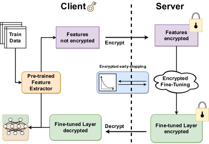
Figure 1: Our privacy-preserving transfer learning protocol (HETAL)

2.2 Homomorphic Encryption: CKKS Scheme

Homomorphic Encryption (HE) is a cryptographic primitive that can support computations on encrypted data without decryption. Particularly, the CKKS scheme (Cheon et al., 2017) is an HE scheme, supporting approximate arithmetic operations over encrypted real and complex numbers. It encrypts multiple complex numbers into a single ciphertext and supports single instruction multiple data (SIMD) operations that perform the same operation simultaneously. The following operations are available for ciphertexts:

• Addition: Element-wise addition of two ciphertexts.

• Multiplication: Element-wise multiplication of two ciphertexts. We denote $\mathsf{Mult}$ for ciphertext-ciphertext multiplication and $\mathsf{CMult}$ for plaintext-ciphertext multiplication (constant multiplication). We also denote $x\odot y$ for the multiplication of $x$ and $y$, irrespective of whether $x$ and $y$ are encrypted. The CKKS scheme is a leveled HE scheme; therefore, we can compute multivariate polynomials of bounded multiplicative depth. It is worth noting that multiplying an arbitrary complex constant also consumes a depth.

• Rotation: For a given plaintext $m=(z_{0},\dots,z_{s-1})\in\mathbb{C}^{s}$ and its ciphertext $\mathsf{ct}$, we can compute $\mathsf{ct_{rot}}=\mathsf{Lrot}(\mathsf{ct},r)$ for $0\leq r<s$, whose decryption is approximately $(z_{r},\dots,z_{s-1},z_{0},\dots,z_{r-1})$.

• Complex conjugation: Element-wise complex conjugation of a ciphertext.

• Bootstrapping: Bootstrapping (Cheon et al., 2018a) is a unique operation that allows us to compute multivariate polynomials of arbitrary degrees. Since bootstrapping is the most expensive computation among all the basic operations in homomorphic encryption, it is crucial to reduce the multiplicative depths of circuits to reduce the number of bootstrapping operations.

2.3 Threat Model

We assume an AutoML-like service, in which a client can outsource model training to a server. The proposed system comprises two parties: one is a client who owns the data and the other is a server that provides ML training services. The protocol aims to allow clients to outsource model training to a server while preserving the privacy of their data. We assume that the server and client can share a pre-trained generic model as a feature extractor, because there are many publicly available pre-trained models, including Vision Transformer (ViT) used in our experiments. During the training task, the client extracts features from its private data using the feature extractor and sends the HE-encrypted features to the server. The server performs fine-tuning for TL on the ciphertext domain and produces an encrypted model.

We assume that the server is honest-but-curious (HBC), where an HBC adversary is a legitimate participant in a communication protocol who will not deviate from the defined protocol but will attempt to learn all possible information from legitimately received messages (Goldreich, 2004). Note that HE provides a good defense to protect the data against an HBC server because the server performs computation over encrypted data without knowing the decryption key.

3 Protocol

3.1 HETAL Protocol

Protocol 1 describes HETAL, which is our privacy-preserving transfer learning protocol. We use superscript ct (resp. pt) when the matrix is encrypted (resp. not encrypted). Note that the client’s data are encrypted using the client’s key, so the server cannot decrypt it, while the server can perform computations using public operation keys. The client extracts features from the input data using a pre-trained model (step 1) and sends the encrypted features to the server (step 2). Then the server fine-tunes a classification layer with encrypted data using NAG, which results in an encrypted fine-tuned layer (step 3). The server sends the encrypted final model to the client and lets the client decrypt and use it for inference (step 4). The server can early-stop the training by computing logits of a validation set and communicating with the client (step 3 (b)-(d)). The client computes the validation loss with the (decrypted) logit and labels and then sends a signal to stop the training if needed, which can prevent overfitting. The client’s data are not revealed to the server because they remain encrypted during the training. Figure 1 shows the overall procedure of HETAL.

We remark that as an alternative to step 4 of our protocol, it is also possible to store the encrypted layer in the server for encrypted inference: the client may send the encrypted features to be classified to the server, receive the encrypted result and decrypt it.

Protocol 1 Protocol of HETAL

1. Using a pre-trained model, the client extracts features from training and validation data. 2. The client encrypts the extracted features and labels of the training set as $\mathcal{B}_{\textsf{train}}^{\textsf{ct}}=\{(\mathbf{X}_{\textsf{train}}^{\textsf{ct}},\mathbf{Y}_{\textsf{train}}^{\textsf{ct}})\}$ and sends them to the server. The client also sends the encrypted features $\mathbf{X}_{\textsf{val}}^{\textsf{ct}}$ of the validation set to the server. 3. For each epoch, repeat the following: (a) For $(\mathbf{X}^{\textsf{ct}},\mathbf{Y}^{\textsf{ct}})\leftarrow\mathcal{B}^{\textsf{ct}}_{\textsf{train}}$, server updates parameters with NAG: W^ct_t+1 = V^ct_t - αN (P^ct - Y^ct)^⊺ X^ct V_t+1^ct = (1 - γ_t)W_t+1^ct + γ_t W_t^ct where $\alpha$ is the learning rate, $N$ is the batch size, $\mathbf{P}^{\textsf{ct}}=\mathsf{ASoftmax}(\mathbf{X}^{\textsf{ct}}(\mathbf{V}^{\textsf{ct}}_{t})^{\operatorname{\intercal}})$ with (row-wise) softmax approximation $\mathsf{ASoftmax}$, and $\{\gamma_{t}\}_{t\geq 0}$ is defined in Section 2.1. (b) With the last weight $\mathbf{W}^{\textsf{ct}}$ in the epoch, the server computes logits $\ell_{\textsf{val}}^{\textsf{ct}}=\mathbf{X}^{\textsf{ct}}_{\textsf{val}}(\mathbf{W}^{\textsf{ct}})^{\operatorname{\intercal}}$ and sends them to the client. (c) The client decrypts the logits and computes the validation loss $\mathcal{L}_{\operatorname{\mathsf{CE}}}$ with $\ell_{\textsf{val}}^{\textsf{pt}}$ and $\mathbf{Y}_{\textsf{val}}^{\textsf{pt}}$. (d) If a loss is not decreased for a fixed number of epochs (patience), then the client sends a signal to the server to stop training. Otherwise, the current best weight $\mathbf{W}^{\textsf{ct}}_{*}$ is replaced with the new weight $\mathbf{W}^{\textsf{ct}}$. 4. The server sends $\mathbf{W}_{*}^{\textsf{ct}}$ to the client, and the client decrypts the parameter and obtains the fine-tuned layer $\mathbf{W}^{\textsf{pt}}_{*}$.

3.2 Security Analysis

We will demonstrate that HETAL protects the client’s data against an HBC server. If the number of training epochs is fixed, the only information a server can see is encrypted features. Therefore, HETAL protects client’s data against HBC server owing to the security of HE. Even when a validation-based early stopping (Step 2 (b) – (d)) is used, only one additional information, i.e., a signal to let the server stop training, is sent to the server, which does not seem to be useful for the server to recover the client’s private data. Additionally, HETAL protects the fine-tuned model from the server because only a client can see it.

In practice, when HETAL is used in AutoML-like MLaaS, the client software may be provided by the server because MLaaS should be available to a non-expert in ML. The client can simply run the software, which applies a pre-trained model to its own data, and then encrypt the extracted features using HE before sending them. However, in this scenario, the client’s data can be secured only if the software is trustworthy. If the source code of the client software can be open to the public, we can apply an approach such as code verification by third parties: for example, see Section 3.1 of (Knauth et al., 2018), stating, “interested parties can inspect the source code to convince themselves.” Therefore, we can ensure the trustworthiness of the HETAL client SW by making them publicly verifiable: it is not harmful for a server to open the source code to public because it consists of a known pre-trained model and encryption function, which are not the server’s secrets.

Finally, we mention that HETAL protects the server’s expertise, such as hyper-parameters and optimized software for training because all training tasks are performed on the server side.

4 Algorithm

In this section, we propose a new softmax approximation algorithm with a much wider range than those in previous studies. In addition, we propose two novel encrypted matrix multiplication algorithms, denoted $\mathsf{DiagABT}$ and $\mathsf{DiagATB}$, which compute matrix multiplications of the forms $AB^{\operatorname{\intercal}}$ and $A^{\operatorname{\intercal}}B$.

4.1 Softmax Approximation

There are several works on the approximation of softmax function with polynomials (Lee et al., 2022b; Hong et al., 2022; Jin et al., 2020). However, all of these methods have low precision (See the Table 3 in the Appendix) and permit only a small domain of approximation, which is not desirable for training with many epochs. We remark that both (Lee et al., 2022b) and (Hong et al., 2022) have been used for inference rather than training.

Regarding the domain of approximation, we experimentally found that the input values of the softmax function increase as training proceeds and easily deviate from the domain that the previous methods can handle. For example, the maximum input value of softmax varies from 0.38 to over 100 on MNIST dataset (Figure 3), which cannot be controlled by the previous approximation methods. Consequently, it is essential to expand the domain of approximation to perform as many training epochs as we want.

To approximate the softmax function on a large interval efficiently, we apply the domain extension technique by (Cheon et al., 2022a). The authors introduced domain extension functions (DEFs) and domain extension polynomials (DEPs) and provided an algorithm to approximate a sigmoid-like functions on exponentially large intervals. More precisely, they provided an algorithm to approximate a DEF that clips an input into a fixed interval as a composition of low-degree polynomials, and applied it to obtain a polynomial that approximates the sigmoid function $\sigma(x)=1/(1+e^{-x})$ on a large interval of scale $[-7683,7683]$. In general, we can approximate a polynomial on a range $[-R,R]$ with $O(\log R)$ complexity.

However, directly applying the domain extension algorithm in (Cheon et al., 2022a) does not constantly work. For example, assume that we have an approximation of a 3-variable softmax on a 3-dimensional box $[-8,8]^{3}$, and an input is given by $(8,10,13)$. Here, the actual value of softmax is $\mathsf{Softmax}(8,10,13)=(0.006,0.047,0.946)$. However, the naive application of the DEF clips the input as $(8,8,8)$ and produces $(0.333,0.333,0.333)$ as an output. A naive application of the method can lead to identical outputs and result in considerable errors. To address the issue, we first normalize input by subtracting maximum value. More precisely, we first compute approximate maximum $m=\mathsf{Amax}(\mathbf{x})$ and set $\mathbf{x}^{\prime}=\mathsf{Norm}(\mathbf{x})=(x_{1}^{\prime},\dots,x_{j}^{\prime})\in\mathbb{R}^{c}$ as $x^{\prime}_{j}=x_{j}-m$ for $1\leq j\leq c$. We use the homomorphic comparison algorithm proposed in (Cheon et al., 2020) to compute $\mathsf{Amax}$ homomorphically as $\mathsf{Amax}(a,b)=a\cdot\mathsf{Acomp}(a,b)+b\cdot(1-\mathsf{Acomp}(a,b))$, with $O(\log c)$ comparisons and rotations, where $\mathsf{Acomp}$ approximates a function $\mathsf{comp}(a,b)$ that returns 1 if $a\geq b$ and 0 otherwise. Then we can easily see that $\mathsf{Softmax}(\mathbf{x}^{\prime})=\mathsf{Softmax}(\mathbf{x})$. Now let $D_{n}:[-L^{n}R,L^{n}R]^{c}\to[-R,R]^{c}$ be a DEP obtained by Algorithm 1 of (Cheon et al., 2022a) with $n$-iterations, where $L$ is a domain extension ratio. The following theorem tells us that, if $p$ is an approximation of the softmax on a small domain, then $\mathsf{ASoftmax}:=p\circ D_{n}\circ\mathsf{Norm}$ gives an approximation of softmax on a large domain. For example, when $R=8$, $L=2$, and $n=5$, $\mathsf{ASoftmax}$ may cover $[-128,128]$, which can handle all steps in Figure 3.

Theorem.

Let $p:\mathbb{R}^{c}\to\mathbb{R}^{c}$ be an approximation of the softmax on $[-R,R]^{c}$ satisfying

$$\|\mathsf{Softmax}(\mathbf{x})-p(\mathbf{x})\|_{\infty}<\epsilon.$$

Then for $\mathbf{x}\in[-\frac{1}{2}L^{n}R,\frac{1}{2}L^{n}R]^{c}$, we have

$$\|\mathsf{Softmax}(\mathbf{x})-p(D_{n}(\mathsf{Norm}(\mathbf{x})))\|_{\infty}<\beta+\epsilon,$$

where $\beta=\beta(\delta,c,r,L,d)$ is a constant that depends only on $\delta,c,r,L,d$.

The proof is stated in Appendix A with a formal version of the theorem. (See Theorem A.6.) The theorem implies that we can approximate softmax on a given domain $[-R_{0},R_{0}]^{c}$ with $O(\log R_{0})$ operations. The precise algorithm can be found in Algorithm 1 in the Appendix.

4.2 Encrypted Matrix Multiplication

We first explain how to encode a matrix into ciphertext(s) and how to perform encrypted matrix multiplications of the forms $AB^{\operatorname{\intercal}}$ and $A^{\operatorname{\intercal}}B$ to compute logits and gradients in HETAL. The main goal of our algorithm is to reduce the number of rotations and multiplications used, which occupy most of the algorithm runtime (see Section 5.1 for the costs of each operation in HE). Note that including a transpose in multiplication is more efficient than computing matrix multiplication of the form $AB$ directly as in (Jiang et al., 2018; Huang et al., 2021), since we need to perform transpose for each iteration of training, which is a costly operation and requires additional multiplicative depth.

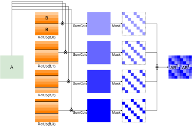
Figure 2: Demonstration of DiagABT algorithm when $A\in\mathbb{R}^{8\times 8}$ and $B\in\mathbb{R}^{4\times 8}$. We do not include the complexification optimization in the figure for simplicity.

4.2.1 Encoding

We used the same encoding method as in (Crockett, 2020), dividing a given matrix as submatrices of a fixed shape $s_{0}\times s_{1}$ and encode each submatrix in the row-major order. Here, each submatrix corresponds to a single ciphertext so that the number of entries in each submatrix equals the number of slots in a single ciphertext, i.e., $s_{0}s_{1}=s$. For convenience, we assume that all matrices are sufficiently small to fit into a single ciphertext. We also assume that the number of rows and columns of the matrices are powers of two by applying zero padding when required. The algorithms can be easily extended to larger matrices (composed of multiple ciphertexts). The details can be found in the Appendix.

4.2.2 Computation of $AB^{\operatorname{\intercal}}$

Let $A\in\mathbb{R}^{a\times b}$ and $B\in\mathbb{R}^{c\times b}$ be two matrices. Our goal is to compute $AB^{\operatorname{\intercal}}\in\mathbb{R}^{a\times c}$ using basic HE operations such as addition, multiplication, and rotation. For this, we use tiling, off-diagonal masking and complexification to reduce the computational complexity.

First, we define some operations and notations. For a given matrix $B$, we define $\operatorname{\mathsf{RotUp}}(B,k)$ as a matrix $B^{\prime}$ obtained by rotating the rows of $B$ in the upper direction by $k$, i.e.,

$$B^{\prime}_{i,j}=B_{(i+k)\,\mathrm{mod}\,c,j}.$$

When $B$ is encoded in a row-wise manner, $\operatorname{\mathsf{RotUp}}(B,k)$ can be obtained from $B$ by simply applying the left rotation of index $kb$, i.e., $\operatorname{\mathsf{RotUp}}(B,k)=\operatorname{\mathsf{Lrot}}(B,kb)$.

Next, for an $s_{0}\times s_{1}$ matrix $X$, we define $\operatorname{\mathsf{SumCols}}(X)$ as a matrix with entries

$$\operatorname{\mathsf{SumCols}}(X)_{i,j}=\sum_{0\leq k<s_{1}}X_{i,k}.$$

In other words, each column of $\operatorname{\mathsf{SumCols}}(X)$ is the sum of the columns in $X$. This can be computed with $2\log s_{1}$ rotations and one constant multiplication: see Algorithm 2 in (Crockett, 2020) for more detail.

We also define matrix $\overline{B}$ as an $s_{0}\times b$ matrix, where $(s_{0}/c)$ copies of $B$ are tiled in the vertical direction. Finally, we define $\overline{B}_{\operatorname{\mathsf{cplx}}}$, complexification of $\overline{B}$, as

$$\overline{B}_{\operatorname{\mathsf{cplx}}}=\overline{B}+\sqrt{-1}\operatorname{\mathsf{RotUp}}(\overline{B},c/2).$$

Note that multiplying $i=\sqrt{-1}$ does not consume a multiplicative depth.

Using the operations defined above, we compute $A\overline{B}^{\operatorname{\intercal}}$ as follows. Note that $A\overline{B}^{\operatorname{\intercal}}$ is a matrix containing $(s_{1}/c)$ copies of $AB^{\operatorname{\intercal}}$ in the horizontal direction.

Proposition 4.1.

Let $A$ and $B$ be defined as above. We have $A\overline{B}^{\operatorname{\intercal}}=X+\operatorname{\mathsf{Conj}}(X)$, where

$$X=\sum_{0\leq k<c/2}\operatorname{\mathsf{SumCols}}(A\odot\operatorname{\mathsf{RotUp}}(\overline{B}_{\operatorname{\mathsf{cplx}}},k))\odot M_{\operatorname{\mathsf{cplx}}}^{(k,c)}.$$

Here $M^{(k,c)}$ is an off-diagonal masking matrix with entries

$$M^{(k,c)}_{i,j}=\begin{cases}1&j\equiv i+k\,(\mathrm{mod}\,c)\\ 0&\text{otherwise}\end{cases}$$

and $M_{\operatorname{\mathsf{cplx}}}^{(k,c)}$ is a complexified version of the mask given by

$$M_{\operatorname{\mathsf{cplx}}}^{(k,c)}=\frac{1}{2}M^{(k,c)}-\frac{\sqrt{-1}}{2}M^{(k+c/2,c)}.$$

Figure 2 illustrates the proposed multiplication method based on Proposition 4.1. The detailed procedure for the proposed algorithm, $\mathsf{DiagABT}$, is presented as Algorithm 2 in the Appendix. Note that the number of rotations is a bottleneck for matrix multiplication, and tiling reduces it from $O(s_{0}\log s_{1})$ to $O(c\log s_{1})$. This also fits into our case for computing $\mathbf{X}\mathbf{W}^{\operatorname{\intercal}}$, because the number of rows of $\mathbf{W}$ equals the number of classes for the dataset, which is often small compared to $s_{0}$ or $s_{1}$. In addition, complexification reduces the complexity by half (a similar idea was used in (Hong et al., 2022)). Finally, we can extend the algorithm to compute $tAB^{\operatorname{\intercal}}$ for $t\in\mathbb{R}$ without additional multiplicative depth consumption by replacing the diagonal mask $M^{(k,c)}_{\operatorname{\mathsf{cplx}}}$ with $tM^{(k,c)}_{\operatorname{\mathsf{cplx}}}$. Algorithm 2 adopts this optimization.

4.2.3 Computation of $A^{\operatorname{\intercal}}B$

We use similar ideas as $AB^{\operatorname{\intercal}}$ for efficient computation of $A^{\operatorname{\intercal}}B$. In addition, we propose a new operation, i.e., partial rotation, to reduce multiplicative depth. Let $A\in\mathbb{R}^{a\times c}$ and $B\in\mathbb{R}^{a\times b}$. We can similarly compute $A^{\operatorname{\intercal}}B$. First, we define $\operatorname{\mathsf{RotLeft}}({A},k)$ as a matrix $A^{\prime}$ obtained by rotating the columns of $A$ in the left direction by $k$, i.e.,

$$A^{\prime}_{i,j}=A_{i,(j+k)\mathrm{mod\,}c}.$$

Unlike $\operatorname{\mathsf{RotUp}}$, this consumes a multiplication depth.

Similar to $\operatorname{\mathsf{SumCols}}$, we can also define $\operatorname{\mathsf{SumRows}}(X)$ for an $s_{0}\times s_{1}$ matrix $X$ as

$$\operatorname{\mathsf{SumRows}}({X})_{i,j}=\sum_{0\leq k<s_{0}}X_{k,j}.$$

In other words, each row of $\operatorname{\mathsf{SumRows}}({X})$ is the sum of the rows in $X$. This can be achieved using with $\log s_{0}$ rotations without additional depth consumption.

As in the case of $AB^{\operatorname{\intercal}}$, we can apply tiling and complexification to reduce the computational complexity. We denote $\underline{A}$ for an $a\times s_{1}$ matrix where $(s_{1}/c)$ copies of $A$ are tiled in the horizontal direction. We also define complexification $\underline{A}_{\operatorname{\mathsf{cplx}}}$ of $\underline{A}$ as

$$\underline{A}_{\operatorname{\mathsf{cplx}}}=\underline{A}+\sqrt{-1}\operatorname{\mathsf{RotLeft}}(\underline{A},c/2).$$

However, since $\operatorname{\mathsf{RotLeft}}$ consumes a multiplicative depth, the level of $\underline{A}_{\operatorname{\mathsf{cplx}}}$ is smaller than that of $\underline{A}$ by one. This may increase the multiplicative depth of $\underline{A}^{\operatorname{\intercal}}B$ by one when the level of $\underline{A}$ is smaller than that of $B$. To address this issue, we propose an algorithm that eventually consumes $B$’s level instead of $A$’s. We first define a new operation $\operatorname{\mathsf{PRotUp}}(-,k)$. For a matrix $B$, $\operatorname{\mathsf{PRotUp}}(B,k)$ is defined as a matrix that the last $k$ columns are rotated upwards by one position. For example, the following figure shows its effect on a matrix of shape $4\times 8$ with $k=3$.

We can compute this homomorphically with a single $\mathsf{CMult}$ and $\operatorname{\mathsf{Lrot}}$, consuming a multiplicative depth (see Algorithm 4 in Appendix). Using this new operation $\operatorname{\mathsf{PRotUp}}$, $\underline{A}^{\operatorname{\intercal}}B$ can be expressed as follows:

Proposition 4.2.

$\underline{A}^{\operatorname{\intercal}}B=X+\operatorname{\mathsf{Conj}}(X)$, where

$$X=\sum_{0\leq k<c/2}\operatorname{\mathsf{SumRows}}(\operatorname{\mathsf{Lrot}}(\underline{A}_{\operatorname{\mathsf{cplx}}},k)\odot\operatorname{\mathsf{PRotUp}}(B,k))\odot M_{\operatorname{\mathsf{cplx}}}^{(-k,a)}.$$

Like $AB^{\operatorname{\intercal}}$, tiling and complexification has an effect of reducing the number of rotations from $O(s_{1}\log s_{0})$ to $O(c\log s_{0})$. Algorithm 5 of Appendix adopts this optimization.

5 Experimental results

5.1 Experimental setup

We used HEaaN (CryptoLab, ), a homomorphic encryption library based on the RNS version of the CKKS scheme (Cheon et al., 2018b), which supports bootstrapping (Cheon et al., 2018a) and GPU acceleration. We take $2^{16}$ as a cyclotomic ring dimension (so that each ciphertext has $s=2^{16-1}=32768$ slots) and ciphertext modulus $q\approx 2^{1555}$, which ensures a 128-bit security level under the SparseLWE estimator (Cheon et al., 2022b).

We used an Intel Xeon Gold 6248 CPU at 2.50GHz, running with 64 threads, and a single Nvidia Ampere A40 GPU. Each operation’s execution time is measured as follows: Add: 0.085 ms, Rotate: 1.2 ms, CMult: 0.9 ms, Mult: 1.6 ms, and Bootstrap: 159 ms.

dataset	encrypted			not encrypted
	Running time		ACC (a)	ACC (b)	ACC loss ((b) - (a))
	Total (s)	Time / Iter (s)
MNIST	3442.29	9.46	96.73%	97.24%	0.51%
CIFAR-10	3114.30	15.72	96.57%	96.62%	0.05%
Face Mask Detection	566.72	4.29	95.46%	95.46%	0.00%
DermaMNIST	1136.99	7.06	76.06%	76.01%	-0.05%
SNIPS	1264.27	6.95	95.00%	94.43%	-0.57%

Table 1: Transfer learning results on 5 benchmark datasets.

5.2 Transfer learning

We used five benchmark datasets for image classification and sentiment analysis: MNIST (Deng, 2012), CIFAR-10 (Krizhevsky et al., 2009), Face Mask Detection (Larxel, 2020), DermaMNIST (Yang et al., 2023), and SNIPS (Coucke et al., 2018). These benchmarks are widely used or private. In addition, We used the pre-trained ViT (Dosovitskiy et al., 2021) (ViT-Base) and MPNet (Song et al., 2020) (MPNet-Base) as feature extractors for image and natural language data, respectively. Both models embed a data point into a single 768-dimensional vector.

The results are shown in Table 1. For early stopping, we set the patience to 3. Table 1 shows that we fine-tuned the encrypted models on all benchmark datasets within an hour. In addition, the accuracy drops of the encrypted models were at most 0.51%, compared to the unencrypted models with the same hyperparameters. (See Table 5 in the Appendix for hyperparameters and the number of epochs for early-stopping.). The time required to transmit logits on the validation datasets is negligible compared to the total execution time, because the total size of ciphertexts for encrypting logits is at most 8.8 MB for each epoch.

We also note that our method scales robustly with larger models, such as ViT-Large that embeds a datapoint into a 1024-dimensional vector (see Appendix C.4 and Table 8).

5.3 Softmax Approximation

In the above experiments, we used our new softmax approximation that covers inputs in the range $[-128,128]$ (See the Appendix for the detailed parameters). To estimate the approximation error, we used Monte Carlo simulation, because it is computationally intractable to find the exact maximum error of functions with many variables. To be precise, we sampled 300 M points on the domain and found that the maximum error was 0.0037–0.0224 and the average error was 0.0022–0.0046 depending on the input dimension. Table 3 in Appendix A.3 shows that these errors are significantly smaller than those of the previous methods.

Figure 3 explains the reason for this improvement. It shows how the minimum and maximum values of input of softmax vary as the training proceeds. The value increases in the order of two, which cannot be handled by previous approximation methods (Lee et al., 2022b; Hong et al., 2022; Jin et al., 2020). This shows that, with the previous approximation methods, it is hard to train a model as much as we want.

Figure 3: Maximum and minimum value of input of softmax at each step (minibatch) for each dataset.

$(a,b,c)$	$AB^{\operatorname{\intercal}}$ ($A\in\mathbb{R}^{a\times b},B\in\mathbb{R}^{c\times b}$)					$A^{\operatorname{\intercal}}B$ ($A\in\mathbb{R}^{a\times c},B\in\mathbb{R}^{a\times b}$)
	(Jin et al., 2020)∗	ColMajor†	DiagABT	Speedup		(Jin et al., 2020)∗	RowMajor†	DiagATB	Speedup
$(128,128,4)$	0.8192	0.1104	0.0601	13.63	1.84	10.0352	0.1171	0.0415	241.81	2.82
$(256,256,8)$	3.2768	0.3203	0.1211	27.06	2.64	40.1408	0.3167	0.1239	323.98	2.56
$(512,769,4)$	4.9216	0.7609	0.1223	40.24	6.22	60.2896	0.7176	0.3343	180.35	2.15
$(1024,769,8)$	9.8432	3.0428	0.3710	26.53	8.20	120.5792	2.8546	1.2558	96.02	2.27
$(2048,769,16)$	19.6864	12.6251	1.2376	15.91	10.20	241.1584	11.8220	4.9970	48.26	2.37

Table 2: Comparison of matrix multiplication algorithms (running time in seconds). ^∗For (Jin et al., 2020), we report estimated running times due to memory issues. The actual number of (constant) multiplications and rotations can be found in Appendix. ^†(Crockett, 2020).

5.4 Encrypted Matrix Multiplication

Matrix multiplication accounted for a large portion of the total training time. For example, when we fine-tuned the model on the CIFAR-10 dataset, the total running time for matrix multiplication took approximately 1712 seconds, which was more than 55% of the total training time. This explains the motivation to develop efficient matrix multiplication algorithms.

We compared our matrix multiplication algorithms with those in (Jin et al., 2020) and (Crockett, 2020), and the results are listed in Table 2. Owing to the memory limitation of the GPU, we could not measure the cost of the algorithms in (Jin et al., 2020), therefore, we report the estimated costs by counting the number of multiplications and rotations. The last three rows correspond to the shapes of the data and parameter matrices in our transfer learning experiments. The table shows that our matrix multiplication algorithms are substantially faster than the baseline algorithms, by 1.8 to 323 times. We emphasize the importance of minimizing both the number of rotations and multiplications in algorithms, even though a single multiplication takes longer than a single rotation. To illustrate this point, consider the computation of $AB^{\intercal}$ with matrices of sizes $A\in\mathbb{R}^{2048\times 769}$ and $B\in\mathbb{R}^{16\times 769}$. With the ColMajor algorithm, this operation requires 784 multiplications but 8703 rotations; hence, the rotation accounts for approximately 90% of the total cost. Our algorithm DiagABT significantly reduces the number of operations to 392 multiplications and 456 rotations and yields a speed increase by a factor of 10.2. Table 7 in Appendix C.3 reports the actual numbers of each operation with various input matrix sizes.

6 Related Work

Softmax Approximation

It is challenging to approximate the softmax function using polynomials in HE. Most previous works could not directly target the softmax but suggest alternative functions. The authors of (Al Badawi et al., 2020) used a quadratic polynomial approximation using the Minimax approximation algorithm. For the exponential function approximation, there was no difference in accuracy between Minimax and $L^{2}$-approximations. The authors of (Lee et al., 2022b) used the Gumbel softmax function instead of the original softmax function to make the input be in the approximation region. In (Hong et al., 2022), the authors used the approximation $\mathsf{AE}_{r,L}(x)=((2^{r}+x)/L)^{2^{r}}$ for the scaled exponential function and combined it with Goldschmidt’s algorithm to obtain an approximation of softmax. However, one must carefully select the scaling factor $L$, which is generally difficult. PrivGD (Jin et al., 2020) trained a model with encrypted data but used one-vs-each softmax (Titsias, 2016) instead and approximated it with a product of degree-3 $L^{2}$-approximations of the sigmoid function.

Encrypted Matrix Multiplication

The algorithms proposed in (Crockett, 2020; Jin et al., 2020) for computing encrypted matrix multiplications of the forms $AB^{\operatorname{\intercal}}$ and $A^{\operatorname{\intercal}}B$ are different from ours. The authors of (Jin et al., 2020) used three different types of packing; Row-majored packing (RP), Column-majored packing (CP), and Replicated packing (REP). A weight matrix was packed with REP, and the input/label matrices were packed with CP. Although the algorithms in (Jin et al., 2020) only consume one multiplicative depth, their computational complexity is significantly higher than that of ours. In addition, their method required many blocks to pack a matrix. In (Crockett, 2020), the author introduced ColMajor and RowMajor algorithms to compute $AB^{\operatorname{\intercal}}$ and $A^{\operatorname{\intercal}}B$, respectively. These algorithms aim to extract and replicate rows/columns and view them as matrix-vector/vector-matrix multiplications. We experimentally showed that the execution times of our algorithms are significantly smaller than that of (Crockett, 2020).

Some encrypted matrix multiplication algorithms (Jiang et al., 2018; Huang et al., 2021) are of the form $AB$, that is, they do not include transpose. As mentioned previously, these are unsuitable for our purpose because they add transpose operations for each training iteration. In addition, we cannot use (Jiang et al., 2018) since the input and weight matrices cannot be packed into a single block.

7 Conclusion

In this study, we proposed HETAL, an efficient HE-based transfer learning algorithm that protects data privacy. We demonstrated its practicality through extensive experiments on five benchmark datasets. We believe that HETAL can be applied to other domains such as speech classification. In addition, our matrix multiplication and softmax approximation can be used for various other purposes, such as the encrypted inference of neural networks with softmax activations.

Appendix A Softmax approximation

A.1 Theoretical error analysis

Lemma A.1.

Let $\mathbf{x}=(x_{1},\dots,x_{c})\in\mathbb{R}^{c}$ be a vector with $\max_{1\leq j\leq c}x_{j}=m\geq 0$. Assume that $x_{i}\leq-r$. Then the $i$-th entry of the output of the softmax is bounded as

$$0<\mathsf{Softmax}(\mathbf{x})_{i}\leq\frac{1}{1+e^{r}}.$$

Proof.

It is clear that the output is positive. For the second inequality, we have

$$\mathsf{Softmax}(x_{1},\dots,x_{c}) =\frac{e^{x_{i}}}{e^{x_{1}}+\cdots+e^{x_{i}}+\cdots+e^{x_{c}}}$$

$$\leq\frac{e^{x_{i}}}{e^{x_{1}}+\cdots+e^{x_{i-1}}+e^{x_{i}}}$$

$$\leq\frac{e^{-r}}{e^{x_{1}}+\cdots+e^{x_{i-1}}+e^{-r}}\qquad\cdots(1)$$

$$\leq\frac{e^{-r}}{1+e^{-r}}=\frac{1}{1+e^{r}}.$$

(When we fix $x_{1},\dots,x_{i-1}$, then the function $x_{i}\mapsto e^{x_{i}}/(e^{x_{1}}+\cdots+e^{x_{i}})$ is increasing and this proves (1).) ∎

Lemma A.2.

For any $\mathbf{x},\mathbf{y}\in\mathbb{R}^{c}$, we have

$$\|\mathsf{Softmax}(\mathbf{x})-\mathsf{Softmax}(\mathbf{y})\|_{\infty}\leq\frac{1}{2}\|\mathbf{x}-\mathbf{y}\|_{\infty}$$

Proof.

Let $g_{i}(t):=\mathsf{Softmax}((1-t)\mathbf{x}+t\mathbf{y})_{i}$ for $t\in\mathbb{R}$ and $1\leq i\leq c$. By the mean value theorem, for each $i$ there exists $t_{i}\in(0,1)$ such that

$$\mathsf{Softmax}(\mathbf{y})_{i}-\mathsf{Softmax}(\mathbf{x})_{i}=\frac{g_{i}(1)-g_{i}(0)}{1-0}=g_{i}^{\prime}(t_{i})=(J_{\mathsf{Softmax}}(\mathbf{z}_{i})(\mathbf{y}-\mathbf{x})^{\operatorname{\intercal}})_{i}$$

where $J_{\mathsf{Softmax}}$ is a Jacobian matrix of softmax and $\mathbf{z}_{i}:=(1-t_{i})\mathbf{x}+t_{i}\mathbf{y}$. By direct computation, one can check that the Jacobian is given by

$$J_{\mathsf{Softmax}}(\mathbf{z}_{i})=\begin{bmatrix}s_{1}-s_{1}^{2}&-s_{1}s_{2}&\cdots&-s_{1}s_{c}\\ -s_{2}s_{1}&s_{2}-s_{2}^{2}&\cdots&-s_{2}s_{c}\\ \vdots&\vdots&\ddots&\vdots\\ -s_{c}s_{1}&-s_{c}s_{2}&\cdots&s_{c}-s_{c}^{2}\end{bmatrix}$$

where $(s_{1},\dots,s_{c})=\mathsf{Softmax}(\mathbf{z}_{i})$. Then we have

$$|\mathsf{Softmax}(\mathbf{y})_{i}-\mathsf{Softmax}(\mathbf{x})_{i}| =|\langle(-s_{i}s_{1},-s_{i}s_{2},\dots,s_{i}-s_{i}^{2},\dots,-s_{i}s_{c}),\mathbf{y}-\mathbf{x}\rangle|$$

$$\leq\|(-s_{i}s_{1},-s_{i}s_{2},\dots,s_{i}-s_{i}^{2},\dots,-s_{i}s_{c})\|_{1}\|\mathbf{y}-\mathbf{x}\|_{\infty}$$

$$=\left(\sum_{j=1}^{c}s_{i}s_{j}+(s_{i}-2s_{i}^{2})\right)\|\mathbf{y}-\mathbf{x}\|_{\infty}$$

$$=2(s_{i}-s_{i}^{2})\|\mathbf{y}-\mathbf{x}\|_{\infty}\leq\frac{1}{2}\|\mathbf{y}-\mathbf{x}\|_{\infty}$$

where the last inequality follows from $\sum_{j=1}^{c}s_{j}=1$ and $2(s_{i}-s_{i}^{2})=\frac{1}{2}-2(s_{i}-\frac{1}{2})^{2}$. This proves the desired inequality. ∎

Lemma A.3.

Let $\mathbf{x}\in\mathbb{R}^{c}$ with $x_{1}\geq x_{2}\geq\cdots\geq x_{c}$ and $x_{1}\geq 0$. For $1\leq k\leq c$, define $\mathbf{x}_{:k}\in\mathbb{R}^{k}$ as $\mathbf{x}_{:k}=(x_{1},\dots,x_{k})$. If $x_{k+1}<-r\leq x_{k}$, for $1\leq i\leq k$ we have

$$0\leq\mathsf{Softmax}(\mathbf{x}_{:k})_{i}-\mathsf{Softmax}(\mathbf{x})_{i}\leq\frac{c-k}{i(c-1+e^{r})}.$$

In particular, we have $0\leq\mathsf{Softmax}(\mathbf{x}_{:k})_{i}-\mathsf{Softmax}(\mathbf{x})_{i}\leq(c-1)/(c-1+e^{r})$.

Proof.

The left inequality is clear. For the right one, we have

$$\mathsf{Softmax}(\mathbf{x}_{:k})_{i}-\mathsf{Softmax}(\mathbf{x})_{i} \leq\frac{e^{x_{i}}}{e^{x_{1}}+\cdots+e^{x_{k}}}-\frac{e^{x_{i}}}{e^{x_{1}}+\cdots+e^{x_{k}}+(c-k)e^{-r}}$$

$$=\frac{e^{x_{i}}}{e^{x_{1}}+\cdots+e^{x_{k}}}\cdot\frac{(c-k)e^{-r}}{e^{x_{1}}+\cdots+e^{x_{k}}+(c-k)e^{-r}}.$$

The first term can be bounded as

$$\mathsf{Softmax}(\mathbf{x}_{:k})_{i}\leq\mathsf{Softmax}(x_{i},x_{i},\dots,x_{i},-r,\dots,-r)_{i}<\frac{1}{i},$$

and the second term can be bounded as

$$\frac{(c-k)e^{-r}}{e^{x_{1}}+\cdots+e^{x_{k}}+(c-k)e^{-r}}\leq\frac{(c-k)e^{-r}}{1+(c-1)e^{-r}}=\frac{c-k}{c-1+e^{r}}.$$

(Here we use $x_{1}\geq 0$ and $x_{2},\dots,x_{k}\geq-r$.) This proves the inequality. ∎

From now, we assume that $d(\cdot)\in\mathscr{D}(\delta,r,R,LR)$ for some $\delta,r,R,L$ with $L>0$ and for $i\geq 1$,

$$d_{0}(x) :=d(x)$$

$$d_{i}(x) :=L^{i}d\left(\frac{x}{L^{i}}\right)$$

$$D_{i}(x) :=(d_{0}\circ d_{1}\circ\dots\circ d_{i-1})(x).$$

Lemma A.4.

Let $d(\cdot)\in\mathscr{D}(\delta,r,R,LR)$. For all $i\geq 1$ and $x\in[-r,r]$, we have $0\leq D_{i}^{\prime}(x)\leq 1$.

Proof.

Use induction on $i$. It is true for $i=1$ by definition ($D_{1}(x)=d(x)$). Assume that we have $0\leq D_{i-1}(x)\leq 1$ for $x\in[-r,r]$. Since $D_{i}(x)=D_{i-1}(d_{i-1}(x))$, we have

$$D_{i}^{\prime}(x)=D_{i-1}^{\prime}(d_{i-1}(x))\cdot d_{i-1}^{\prime}(x)=D_{i-1}^{\prime}(d_{i-1}(x))\cdot d^{\prime}\left(\frac{x}{L^{i-1}}\right).$$

Now combining the induction hypothesis with $d_{i-1}(x)\in[-r,r]$ and $x/L^{i-1}\in[-r,r]$ results that the above expression lies between 0 and 1. ∎

The following lemma gives a lower bound of $D_{n}(x)$ for $x\in[-r,r]$ that does not depend on $n$.

Lemma A.5.

For all $n\geq 1$ and $x\in[0,r]$, we have

$$D_{n}(x)\geq x-\frac{\delta L^{2}}{L^{2}-1}x^{3}.$$

Proof.

By mean value theorem, for each $i\geq 2$, we have

$$D_{i-1}(x)-D_{i}(x) =D_{i-1}(x)-D_{i-1}(d_{i-1}(x))$$

$$=D_{i-1}^{\prime}(c)(x-d_{i-1}(x))\qquad\qquad(\text{for some }d_{i-1}(x)<c<x)$$

$$\leq x-d_{i-1}(x)$$

$$=L^{i-1}\left(\frac{x}{L^{i-1}}-d\left(\frac{x}{L^{i-1}}\right)\right)$$

$$\leq L^{i-1}\cdot\delta\left(\frac{x}{L^{i-1}}\right)^{3}=\frac{\delta}{L^{2(i-1)}}$$

where the first inequality follows from Lemma A.4. Hence we get

$$D_{n}(x) =x-(x-D_{1}(x))-(D_{1}(x)-D_{2}(x))-\cdots-(D_{n-1}(x)-D_{n}(x))$$

$$\geq x-\left(\delta x^{3}+\frac{\delta}{L^{2}}x^{3}+\cdots+\frac{\delta}{L^{2(n-1)}}x^{3}\right)$$

$$=x-\delta\frac{1-L^{-2n}}{1-L^{-2}}x^{3}$$

$$\geq x-\frac{\delta L^{2}}{L^{2}-1}x^{3}.$$

∎

Now we prove our main theorem.

Theorem A.6.

Let $d(\cdot)\in\mathscr{D}(\delta,r,R,LR)$ be a DEP and abuse a notation so that $d:\mathbb{R}^{c}\to\mathbb{R}^{c}$ is a function that applies $d:\mathbb{R}\to\mathbb{R}$ component-wise. Let $p:[-R,R]^{c}\to[-R,R]^{c}$ be a polynomial approximation of $\mathsf{Softmax}$ with minimax error $\|\mathsf{Softmax}(\mathbf{x})-p(\mathbf{x})\|_{\infty}<\epsilon$. Let $\mathsf{Amax}:[-L^{n}R,L^{n}R]^{c}\to[-L^{n}R,L^{n}R]^{c}$ be a given polynomial appproximation of max function satisfying $\mathsf{Amax}(\mathbf{x})\leq\mathsf{max}(\mathbf{x})$ and $\|\mathsf{Amax}(\mathbf{x})-\mathsf{max}(\mathbf{x})\|_{\infty}\leq r$. Define a normalized vector $\mathbf{x}^{\prime}=\mathrm{Norm}(\mathbf{x})=(x_{1}^{\prime},\dots,x_{c}^{\prime})\in\mathbb{R}^{c}$ as $x^{\prime}_{j}=x_{j}-m$ for $1\leq j\leq c$, where $m=\mathsf{Amax}(\mathbf{x})$. For $p_{n}:=p\circ D_{n}$ with $D_{n}:=d_{0}\circ\cdots\circ d_{n-1}$ and $d_{i}(x):=L^{i}d(x/L^{i})$, if $\mathbf{x}\in[-\frac{1}{2}L^{n}R,\frac{1}{2}L^{n}R]^{c}$, we have

$$\|\mathsf{Softmax}(\mathbf{x})-p_{n}(\mathbf{x}^{\prime})\|_{\infty}<\beta(c,\delta,r,L,d)+\epsilon$$

where

$$\beta(c,\delta,r,L,d):=\frac{1}{1+\frac{e^{r}}{c-1}}+\frac{1}{1+\frac{e^{r-\delta L^{2}r^{3}/(L^{2}-1)}}{c-1}}+\frac{\delta r^{3}L^{2}}{2(L^{2}-1)}.$$

Note that the upper bound does not depend on $n$.

Proof.

One can assume that $x_{1}\geq x_{2}\geq\cdots\geq x_{c}$. By the assumption on $\mathsf{ApproxMax}$, $x_{c}\leq m\leq x_{1}$ and $r\geq x_{1}^{\prime}=x_{1}-m\geq 0$. In other words, $\mathbf{x}^{\prime}\in[-L^{n}R,r]^{c}$. Since $\mathsf{Softmax}(\mathbf{x}^{\prime})=\mathsf{Softmax}(\mathbf{x})$, we have. We have

$$\|\mathsf{Softmax}(\mathbf{x})-p_{n}(\mathbf{x^{\prime}})\|_{\infty} =\|\mathsf{Softmax}(\mathbf{x}^{\prime})-p_{n}(\mathbf{x}^{\prime})\|_{\infty}$$

$$\leq\|\mathsf{Softmax}(\mathbf{x}^{\prime})-\mathsf{Softmax}\circ D_{n}(\mathbf{x}^{\prime})\|_{\infty}+\|\mathsf{Softmax}\circ D_{n}(\mathbf{x}^{\prime})-p\circ D_{n}(\mathbf{x}^{\prime})\|_{\infty}$$

For $1\leq i\leq c$, if $x_{i}^{\prime}\leq-r$, then by Lemma A.1, we have

$$0<\mathsf{Softmax}(\mathbf{x}^{\prime})_{i}\leq\frac{1}{1+e^{r}},\quad 0<\mathsf{Softmax}(D_{n}(\mathbf{x}^{\prime}))_{i}\leq\frac{1}{1+e^{D_{n}(r)}}.$$

(Second inequality follows from $D_{n}(x_{1}^{\prime})\geq 0$ and $D_{n}(x_{i}^{\prime})\leq-D_{n}(r)$.) If $x_{i}^{\prime}\geq-r$, let $k\in\{1,\dots,c\}$ be a minimal number such that $x_{k}^{\prime}\geq-r$, so that $x_{c}^{\prime}\leq\cdots\leq x_{k+1}^{\prime}<-r\leq x_{k}^{\prime}\leq\cdots\leq x_{1}^{\prime}$. Let $\mathbf{x}_{:k}^{\prime}:=(x_{1}^{\prime},\dots,x_{k}^{\prime})\in\mathbb{R}^{k}$. Then

$$|\mathsf{Softmax}(\mathbf{x}^{\prime})_{i}-\mathsf{Softmax}(D_{n}(\mathbf{x}^{\prime}))_{i}| \leq|\mathsf{Softmax}(\mathbf{x}^{\prime})_{i}-\mathsf{Softmax}(\mathbf{x}_{:k}^{\prime})_{i}|$$

$$+|\mathsf{Softmax}(\mathbf{x}_{:k}^{\prime})_{i}-\mathsf{Softmax}(D_{n}(\mathbf{x}_{:k}^{\prime}))_{i}|$$

$$+|\mathsf{Softmax}(D_{n}(\mathbf{x}_{:k}^{\prime}))_{i}-\mathsf{Softmax}(D_{n}(\mathbf{x}^{\prime}))_{i}|.$$

By Lemma A.3, the first and third terms are bounded above by $(c-1)/(c-1+e^{r})$ and $(c-1)/(c-1+e^{D_{n}(r)})$, respectively. The second term can be bounded using Lemma A.2 and Theorem 1 of (Cheon et al., 2022a) as

$$|\mathsf{Softmax}(\mathbf{x}^{\prime}_{:k})_{i}-\mathsf{Softmax}(D_{n}(\mathbf{x}^{\prime}_{:k}))_{i}|\leq\frac{1}{2}\|\mathbf{x}^{\prime}_{:k}-D_{n}(\mathbf{x}^{\prime}_{:k})\|_{\infty}\leq\frac{\delta r^{3}L^{2}}{2(L^{2}-1)}.$$

Hence we get

$$|\mathsf{Softmax}(\mathbf{x}^{\prime})_{i}-\mathsf{Softmax}(D_{n}(\mathbf{x}^{\prime}))_{i}|\leq\beta(c,\delta,r,L,d).$$

Since $1/(1+e^{r})\leq 1/(1+e^{r}/(c-1))<\beta(c,\delta,r,L,d)$ and $1/(1+e^{D_{n}(r)})\leq 1/(1+e^{D_{n}(r)}/(c-1))\leq 1/({1+e^{r-\delta L^{2}r^{3}/(L^{2}-1)}}/(c-1))<\beta(c,\delta,r,L,d)$, we get

$$\|\mathsf{Softmax}(\mathbf{x}^{\prime})-\mathsf{Softmax}(D_{n}(\mathbf{x}^{\prime}))\|_{\infty}\leq\beta(c,\delta,r,L,d).$$

For the other term, since $D_{n}(\mathbf{x}^{\prime})\in[-R,R]^{c}$, we have $\|\mathsf{Softmax}(D_{n}(\mathbf{x}^{\prime}))-p(D_{n}(\mathbf{x}^{\prime}))\|_{\infty,[-L^{n}R,L^{n}R]^{c}}<\epsilon$. By combining these, we get the inequality. ∎

A.2 Algorithm

Based on our softmax approximation, Algorithm 1 computes the row-wise softmax of a matrix $M\in\mathbb{R}^{a\times c}$, which gives $\mathbf{P}\in\mathbb{R}^{a\times c}$ when given $M=\mathbf{X}\mathbf{W}^{\operatorname{\intercal}}$, the probability matrix for each input in a minibatch. Here $\mathsf{AExp}$ and $\mathsf{AInv}$ are approximated exponential and inverse functions with the algorithms in (Lee et al., 2022b), with our modified parameters. Also $\langle{M}\rangle$ stands for the encoding of a matrix $M$ with submatrices of size $s_{0}\times s_{1}$ - see Appendix B for the details. Note that the $\mathbf{X}\mathbf{W}^{\operatorname{\intercal}}$ is tiled horizontally (assuming that the matrix $\mathbf{W}$ is zero-padded and tiled vertically), and we also want that the result of softmax is tiled horizontally, to apply our matrix multiplication algorithm. Line 1–19 corresponds to the normalization of input that computes a row-wise max and subtracts it from the input. The loop in line 21–27 is the domain extension step, where line 24–27 yields a high accuracy. After computing the softmax (line 28–32), line 33–35 make the result matrix tiled horizontally. For the comparison function, we followed the algorithm in (Cheon et al., 2020). More precisely, we approximate $x\mapsto(\mathsf{sgn}(x)+1)/2$ on $[-1,1]$ as a polynomial $f(g(g(x)))$ where

$$f(x)=-\frac{5}{16}\left(x^{7}-\frac{21}{5}x^{5}+7x^{3}-7x\right),\quad g(x)=-\frac{12860}{1024}\left(x^{7}-\frac{25614}{12860}x^{5}+\frac{16577}{12860}x^{3}-\frac{4589}{12860}x\right),$$

and get an approximation for $\mathsf{comp}(a,b):=(\mathsf{sgn}(a-b)+1)/2$ with $-1/2\leq a,b\leq 1/2$. Note that increasing the number of compositions of $f$ and $g$ gives a better approximation of the comparison. However, we have experimentally found that $f(g(g(x))$ is enough for our experiments.

Algorithm 1 Row-wise softmax approximation

Input: $\langle{\underline{M}}\rangle$, for $M\in\mathbb{R}^{a\times c}$, $c\leq s_{1}$, $c^{\prime}=2^{\lceil\log_{2}c\rceil}$, $R_{\mathsf{orig}}$ (original approximation range), $L$ (domain extension ratio), $n$ (domain extension index), $\mathsf{Acomp}(\cdot,\cdot)$ (homomorphic approximate comparison function), precise (boolean).
Output: $\langle{\underline{\mathsf{ASoftmax}(M)}}\rangle$

1:  $R_{\mathsf{max}}=\lceil R_{\mathsf{orig}}\cdot L^{n}\rceil$

2:  $D_{c}=(d_{ij})$ where

$$d_{ij}=\begin{cases}1&0\leq j<c\\ 0&\text{otherwise}\end{cases}$$

3:  $\langle{M^{\prime}}\rangle=\langle{\underline{M}}\rangle\times\left(\frac{1}{2R_{\mathsf{max}}}\right)$

4:  if $c\neq c^{\prime}$ then

5:     $D_{\mathsf{padmask}}=(m_{ij})$ where

$$m_{ij}=\begin{cases}0&0\leq j<c\\ 1/2&\text{otherwise}\end{cases}$$

6:     $\langle{M^{\prime}}\rangle=\langle{M^{\prime}}\rangle-\langle{D_{\mathsf{padmask}}}\rangle$

7:  end if

8:  $D_{\mathsf{firstcol}}=(m_{ij}^{\prime})$ where

$$m_{ij}^{\prime}=\begin{cases}1&j=0\\ 0&\text{otherwise}\end{cases}$$

9:  for $j=0$ to $\log_{2}(c^{\prime})$ do

10:     $\langle{M_{\mathsf{rot}}}\rangle=\mathsf{Lrot}(\langle{M_{\mathsf{max}}}\rangle,2^{j})$

11:     $\langle{M_{\mathsf{comp}}}\rangle=\mathsf{Acomp}(\langle{M_{\mathsf{max}}}\rangle,\langle{M_{\mathsf{rot}}}\rangle)$

12:     $\langle{M_{\mathsf{max}}}\rangle=\langle{M_{\mathsf{max}}}\rangle\odot\langle{M_{\mathsf{comp}}}\rangle+\langle{M_{\mathsf{rot}}}\rangle\odot(1-\langle{M_{\mathsf{comp}}}\rangle)$

13:  end for

14:  $\langle{M_{\mathsf{max}}}\rangle=\langle{M_{\mathsf{max}}}\rangle\cdot\langle{D_{\mathsf{firstcol}}}\rangle$

15:  for $j=0$ to $\log_{2}(s_{1})$ do

16:     $\langle{M_{\mathsf{max}}}\rangle=\langle{M_{\mathsf{max}}}\rangle+\mathsf{Rrot}(\langle{M_{\mathsf{max}}}\rangle,2^{i}\cdot s_{1})$

17:  end for

18:  $\langle{M_{\mathsf{max}}}\rangle=\langle{M_{\mathsf{max}}}\rangle\times(2R_{\mathsf{max}})$

19:  $\langle{{M_{\mathsf{norm}}}}\rangle=(\langle{\underline{M}}\rangle-\langle{{M_{\mathsf{max}}}}\rangle)\odot\langle{D_{c}}\rangle$

20:  $B(x):=x-\frac{4x^{3}}{27R_{\mathsf{orig}}^{2}}$

21:  for $i=n-1$ to 0 do

22:     $\langle{{M_{\mathsf{norm}}}}\rangle=L^{i}\odot B(\langle{{M_{\mathsf{norm}}}}\rangle\odot L^{-i})$

23:  end for

24:  if precise then

25:     $B_{\mathsf{inv}}(x):=x-\frac{4}{27}\frac{L^{2}(L^{2n}-1)}{L^{2n}(L^{2}-1)}\left(\frac{x^{3}}{R_{\mathsf{orig}}^{2}}-\frac{x^{5}}{R_{\mathsf{orig}}^{4}}\right)$

26:     $\langle{M_{\mathsf{norm}}}\rangle=B_{\mathsf{inv}}(\langle{M_{\mathsf{norm}}}\rangle)$

27:  end if

28:  $M_{\mathsf{exp}}=\mathsf{AExp}(\langle{{M_{\mathsf{norm}}}}\rangle)$

29:  $M_{\mathsf{exp}}=M_{\mathsf{exp}}\odot\langle{D_{c}}\rangle$

30:  $M_{\mathsf{expsum}}=\operatorname{\mathsf{SumRows}}(M_{\mathsf{exp}})$

31:  $M_{\mathsf{Z}}=\mathsf{AInv}(M_{\mathsf{expsum}})$

32:  $M_{\mathsf{Softmax}}=M_{\mathsf{expsum}}\odot M_{\mathsf{Z}}$

33:  for $j=0$ to $\log_{2}(s_{1}/c^{\prime})$ do

34:     $M_{\mathsf{Softmax}}=M_{\mathsf{Softmax}}+\operatorname{\mathsf{Rrot}}(M_{\mathsf{Softmax}},2^{j}\cdot s_{1}\cdot c^{\prime})$

35:  end for

36:  $\langle{\underline{\mathsf{ASoftmax}(M)}}\rangle=M_{\mathsf{Softmax}}$

A.3 Comparison with previous approaches

The following Table 3 shows the maximum and average errors of the softmax approximations including (Lee et al., 2022b; Hong et al., 2022; Jin et al., 2020) and ours, for each input dimension $c$ and range $R$. Since it is computationally intractable to find the exact maximum error of functions in several variables, we randomly sample points on each domain of approximation instead and report its maximum. More precisely, according to the value of $R$, we sample as

• $R=4$: sample 100M points uniformly on $[-4,4]^{c}$,

• $R=8$: sample 100M points on $[-4,4]^{c}$ and $[-8,8]^{c}$ uniformly, total 200M points,

• $R=32$: sample 100M points on $[-4,4]^{c}$, $[-8,8]^{c}$, and $[-32,32]^{c}$ uniformly, total 300M points.

• $R=128$: sample 100M points on $[-4,4]^{c}$, $[-8,8]^{c}$, $[-32,32]^{c}$, and $[-128,128]^{c}$ uniformly, total 400M points.

(we sample the points in such an accumulative way since uniformly randomly sampled points become more sparse as $R$ increases, so we additionally sample points on smaller intervals to consider possible large error on small intervals, too.) We can see that our approximation could cover the widest range with smallest error. When the error is too large (e.g. Goldschmidt’s algorithm fail to converge due to large input value), we filled up the corresponding entry with -.

For the comparison, we use the following parameters.

• (Lee et al., 2022b): We use the same parameters given in the paper. In particular, we use degree 12 $L^{2}$-approximation of the exponential function on $[-1,1]$ with $B=64$, $R=10000$ and $n=8$ for inverse approximation, and Gumbel softmax function is used with $\lambda=4$.

• (Hong et al., 2022): We use the same parameters given in the paper. In particular, we use $(r,L)=(4,32)$ for $\mathsf{AExp}_{r,L}$ and $M=80$ and $d=30$ for inverse (which are the same as $R=80$ and $d=30$ if we use the notations from (Lee et al., 2022b)).

• (Jin et al., 2020): They used degree 3 $L^{2}$-approximation of sigmoid on $[-8,8]$ (that is $y=0.5+0.15012x-0.00159x^{3}$, used in (Kim et al., 2018b)) which has a minimax error of 0.0098 on $[-8,8]$. So we have observed the resulting one-vs-each softmax approximation error on $[-4,4]^{c}$. (Since we take differences between inputs for each class, the actual input of each sigmoid could fit into $[-8,8]$ when the input themselves are in $[-4,4]$.)

• Ours: Our initial softmax approximation is based on (Lee et al., 2022b), but with different parameters. We use $B=8$ for exponential (approximation on $[-8,8]$) and $R=100$ and $n=16$ for inverse. Since normalization subtracts (approximate) maximum value from inputs, the possible range of the resulting normalized input becomes twice; hence our softmax can only cover $[-4,4]^{c}$ without domain extension. For domain extension, we set the domain extension ratio as $L=2$ and domain extension index as $5$, so that the new domain of approximation becomes $[-128,128]^{c}$. Also, we can increase precision by applying Algorithm 2 of (Cheon et al., 2020) which applies an additional degree 5 polynomial which approximates the inverse of DEP.

$c$	$R$	(Lee et al., 2022b)		(Hong et al., 2022)		(Jin et al., 2020)		Ours (norm)		Ours (norm+extn)		Ours (norm+extn+prec)
3	4	0.9243	0.6957	0.0755	0.0162	0.1841	0.0910	3.7e-7	4.3e-8	0.0037	0.0015	0.0013	0.0003
	8	0.9651	0.7131	0.6041	0.0199	-	-	-	-	0.0037	0.0015	0.0013	0.0004
	32	0.9997	0.5812	-	-	-	-	-	-	0.0037	0.0015	0.0022	0.0006
	128	-	-	-	-	-	-	-	-	0.0037	0.0014	0.0022	0.0006
5	4	0.9138	0.5784	0.0965	0.0239	0.3093	0.1148	7.2e-7	7.4e-8	0.0071	0.0029	0.0026	0.0004
	8	0.9591	0.5320	0.4121	0.0313	-	-	-	-	0.0071	0.0029	0.0026	0.0005
	32	0.9996	0.4806	-	-	-	-	-	-	0.0071	0.0024	0.0044	0.0008
	128	-	-	-	-	-	-	-	-	0.0116	0.0023	0.0044	0.0010
7	4	0.9051	0.4926	0.1030	0.0297	0.4930	0.1296	1.0e-6	9.1e-8	0.0065	0.0031	0.0026	0.0003
	8	0.9522	0.5320	0.2095	0.0416	-	-	-	-	0.0073	0.0029	0.0030	0.0005
	32	0.9992	0.4252	-	-	-	-	-	-	0.0087	0.0029	0.0065	0.0010
	128	-	-	-	-	-	-	-	-	0.0089	0.0029	0.0066	0.0013
10	4	0.8942	0.3992	0.0948	0.0339	0.8018	0.1501	1.4e-6	1.0e-7	0.0153	0.0046	0.0040	0.0006
	8	0.9438	0.4476	0.2167	0.0516	-	-	-	-	0.0153	0.0042	0.0050	0.0014
	32	0.9985	0.3768	-	-	-	-	-	-	0.0153	0.0039	0.0094	0.0012
	128	-	-	-	-	-	-	-	-	0.0224	0.0039	0.0097	0.0016

Table 3: Maximum and average errors of softmax approximation with 100–300M sampled points. Ours (norm+extn+prec) represents our approach combined with Algorithm 2 of (Cheon et al., 2022a).

The errors of previous works are fairly large, considering that softmax values lie between 0 and 1, and one can ask if it is possible to use these approximations in practice. The authors of (Lee et al., 2022a). (resp. (Hong et al., 2022)) proposed a softmax approximation and showed it is useful for ResNet-20 inference (resp. shallow neural network), where it is sufficient to identify the largest of many values rather than to calculate the exact values. This explains why their approximation works well for their purpose. However, for training, we need a softmax approximation that works well uniformly on large intervals; therefore, previous algorithms are not exactly suitable for training. Although the one-vs-rest softmax is used for training in (Jin et al., 2020), the input range is limited to $[-4,4]$.

A.4 Softmax input with vanilla SGD training

Figure 4: Maximum and minimum value of input of softmax at each step (minibatch) for each dataset, where the model is trained with vanilla SGD.

Figure 4 shows how the minimum and maximum values of input of softmax vary as training proceeds when we use vanilla SGD instead of NAG. Although the input values increase slower than that with NAG, the values are still significant and cannot be covered by the previous softmax approximation methods. (Note that it took about 10 times longer than NAG to train models.)

Appendix B Encrypted matrix multiplication

B.1 Matrix composed of multiple blocks

In the main article, we assumed that each matrix could fit into a single block (message or ciphertext) to simplify explanations. Now we give a detailed description of the matrix multiplication algorithms for matrices whose encodings are composed of multiple blocks.

Let $A\in\mathbb{R}^{a\times b}$ be a matrix. Fix a unit matrix shape $s_{0}\times s_{1}$, where $s=s_{0}s_{1}$ equals the number of slots in a single ciphertext. When $a\leq s_{0}$ and $b\leq s_{1}$, we apply zero-padding to the right end and bottom of $A$ and encode it into a single block in a row-major manner. $\langle{A}\rangle$ denotes this encoding. For example, if $a=b=3$ and $s_{0}=s_{1}=4$, the matrix $A=(a_{ij})_{0\leq i,j<3}$ is encoded as

$$\langle{A}\rangle=(a_{00},a_{01},a_{02},0,a_{10},a_{11},a_{12},0,a_{20},a_{21},a_{22},0,0,0,0,0).$$

If $a>s_{0}$ or $b>s_{1}$, we first zero-pad $A$ so that the number of rows and columns are multiples of $s_{0}$ and $s_{1}$, respectively, and then split $A$ into submatrices of shape $s_{0}\times s_{1}$. Then encoding each submatrix gives an encoding $\langle{A}\rangle$ of $A$,

$$\langle{A}\rangle=\{\langle{A}\rangle_{i,j}\}_{0\leq i<\lceil a/s_{0}\rceil,0\leq j<\lceil b/s_{1}\rceil},$$

where $\langle{A}\rangle_{i,j}$ is the encoding of $(i,j)$-th submatrix. (See also Figure 5.) As explained in (Crockett, 2020), we can extend the $\operatorname{\mathsf{SumRows}}$ and $\operatorname{\mathsf{SumCols}}$ algorithm for large matrices.

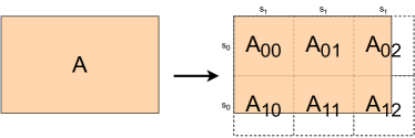
Figure 5: Encoding of a matrix $A\in\mathbb{R}^{13\times 21}$ into 6 blocks where each encoded matrix of unit shape $8\times 8$.

B.2 Proofs

Here we give proofs for the propositions on encrypted matrix multiplication algorithms.

Proposition B.1.

Let $A,B$ as above. We have $A\overline{B}^{\operatorname{\intercal}}=X+\operatorname{\mathsf{Conj}}(X)$ where

$$X=\sum_{0\leq k<c/2}\operatorname{\mathsf{SumCols}}(A\odot\operatorname{\mathsf{RotUp}}(\overline{B}_{\operatorname{\mathsf{cplx}}},k))\odot M_{\operatorname{\mathsf{cplx}}}^{(k,c)}.$$ (1)

Here $M^{(k,d)}$ is an off-diagonal masking matrix with entries

$$M^{(k,d)}_{i,j}=\begin{cases}1&j\equiv i+k\,(\mathrm{mod}\,d)\\ 0&\text{otherwise}\end{cases}$$

and $M_{\operatorname{\mathsf{cplx}}}^{(k,c)}$ is a complexified version of the mask, which is

$$M_{\operatorname{\mathsf{cplx}}}^{(k,c)}=\frac{1}{2}M^{(k,c)}-\frac{\sqrt{-1}}{2}M^{(k+c/2,c)}$$

Proof.

We will first show that

$$A\overline{B}^{\operatorname{\intercal}}=\sum_{0\leq k<c}\operatorname{\mathsf{SumCols}}(A\odot\operatorname{\mathsf{RotUp}}(\overline{B},k))\odot M^{(k,c)}.$$ (2)

It is enough to show that the $(i,j)$-th entry of the right-hand side equals $\mathbf{a}_{i}\mathbf{b}_{j}^{\operatorname{\intercal}}$, where $\mathbf{a}_{i}$ (resp. $\mathbf{b}_{j}$) is $i$-th (resp. $j$-th) row of $A$ (resp. $\overline{B}$). Choose $0\leq k_{0}<c$ such that $j-i\equiv k_{0}\,(\mathrm{mod}\,c)$. Then all the $(i,j)$-th entries of summands of the right hand side vanishes except for the summand with index $k=k_{0}$ because of the masking. For $k=k_{0}$, the $(i,j)$-th entry equals the dot product of the $i$-th row of $A$ and the $i$-th row of $\operatorname{\mathsf{RotUp}}(B,k_{0})$, and the latter is $i+k_{0}\equiv j$-th row of $B$.

Now, we can see that

$$\operatorname{\mathsf{RotUp}}({\overline{B}_{\operatorname{\mathsf{cplx}}}},k)=\operatorname{\mathsf{RotUp}}({\overline{B}},k)+\sqrt{-1}\operatorname{\mathsf{RotUp}}({\overline{B}},k+c/2)$$

and by the linearity of $\operatorname{\mathsf{SumCols}}$ and bi-linearity of $\odot$, we get

$$\operatorname{\mathsf{SumCols}}(A\odot\operatorname{\mathsf{RotUp}}(\overline{B}_{\operatorname{\mathsf{cplx}}},k))=\operatorname{\mathsf{SumCols}}(A\odot\operatorname{\mathsf{RotUp}}(\overline{B},k))+\sqrt{-1}\operatorname{\mathsf{SumCols}}(A\odot\operatorname{\mathsf{RotUp}}(\overline{B},k+c/2)).$$

Now, combining this with equation,

$$\Re((x+zi)(y-wi))=xy+zw,\quad x,y,z,w\in\mathbb{R},$$

we get

$$2\Re(\operatorname{\mathsf{SumCols}}(A\odot\operatorname{\mathsf{RotUp}}(\overline{B}_{\operatorname{\mathsf{cplx}}},k))\odot M_{\operatorname{\mathsf{cplx}}}^{(k,c)})$$

$$=\operatorname{\mathsf{SumCols}}(A\odot\operatorname{\mathsf{RotUp}}(\overline{B},k))\odot M^{(k,c)}$$

$$+\operatorname{\mathsf{SumCols}}(A\odot\operatorname{\mathsf{RotUp}}(\overline{B},k+c/2))\odot M^{(k+c/2,c)}.$$

In other words, the $k$-th summand of Equation (1) equals to the sum of the $k$-th and $(k+c/2)$-th summands of Equation (2), and this completes the proof. ∎

Proposition B.2.

$\underline{A}^{\operatorname{\intercal}}B=X+\mathsf{conj}(X)$, where

$$X=\sum_{0\leq k<c/2}\operatorname{\mathsf{SumRows}}(\operatorname{\mathsf{Lrot}}(\underline{A}_{\operatorname{\mathsf{cplx}}},k)\odot\operatorname{\mathsf{PRotUp}}(B,k))\odot M_{\operatorname{\mathsf{cplx}}}^{(-k,c)}.$$

Proof.

Once we show the following identity

$$\operatorname{\mathsf{SumRows}}(\operatorname{\mathsf{Lrot}}(\underline{A}_{\operatorname{\mathsf{cplx}}},k)\odot\operatorname{\mathsf{PRotUp}}(B,k))=\operatorname{\mathsf{SumRows}}(\operatorname{\mathsf{RotLeft}}(\underline{A}_{\operatorname{\mathsf{cplx}}},k)\odot B),$$

our equation is equivalent to

$$X=\sum_{0\leq k<c/2}\operatorname{\mathsf{SumRows}}(\operatorname{\mathsf{RotLeft}}(\underline{A}_{\operatorname{\mathsf{cplx}}},k)\odot B)\odot M_{\operatorname{\mathsf{cplx}}}^{(-k,c)}.$$

which can be proved in a similar way as Proposition 2. We can check that the first $(b-k)$ columns of $\operatorname{\mathsf{RotLeft}}^{*}(\underline{A}_{\operatorname{\mathsf{cplx}}},k)$ coincide with them of $\operatorname{\mathsf{RotLeft}}(\underline{A}_{\operatorname{\mathsf{cplx}}},k)$, and same thing holds for $\operatorname{\mathsf{PRotUp}}(B,k)$ and $B$. The last $k$ columns of $\operatorname{\mathsf{RotLeft}}^{*}(\underline{A}_{\operatorname{\mathsf{cplx}}},k)\odot\operatorname{\mathsf{PRotUp}}(B,k)$ are

$$\begin{bmatrix}x_{2,1}\cdot y_{2,b-k+1}&\dots&x_{2,k}\cdot y_{2,b}\\ x_{3,1}\cdot y_{3,b-k+1}&\dots&x_{3,k}\cdot y_{3,b}\\ \vdots&\ddots&\vdots\\ x_{1,1}\cdot y_{1,b-k+1}&\dots&x_{1,k}\cdot y_{1,b}\\ \end{bmatrix}$$

where $\underline{A}_{\operatorname{\mathsf{cplx}}}=(x_{i,j})$ and $B=(y_{i,j})$, and the sums of entries in each column equal to them of $\operatorname{\mathsf{RotLeft}}(\underline{A}_{\operatorname{\mathsf{cplx}}})\odot B$. ∎

B.3 Algorithms

We give detailed algorithms that we used for computing encrypted matrix multiplications. It is worth noting that there are some restrictions on the shape of matrices and unit matrices for encoding. For example, Algorithm 2 requires that the number of rows $c$ of $B$ should satisfy $1<c\leq s_{0}$. Hence we set the unit matrix shape $s_{0},s_{1}$ to satisfy the restriction for the actual implementation.

We first briefly explain how the operations like addition, multiplication, $\operatorname{\mathsf{SumRows}}$, $\operatorname{\mathsf{SumCols}}$, $\operatorname{\mathsf{Lrot}}$, and $\operatorname{\mathsf{Rrot}}$ are extended to encodings composed of several blocks, i.e. when

$$\langle{A}\rangle=\{\langle{A}\rangle_{i,j}\}_{0\leq i<m,0\leq j<n}.$$

Addition and multiplication are simple. Let $\langle{A_{1}}\rangle=\{\langle{A_{1}}\rangle_{i,j}\}_{0\leq i<m_{1},0\leq j<n_{1}}$ and $\langle{A_{2}}\rangle=\{\langle{A_{2}}\rangle_{i,j}\}_{0\leq i<m_{2},0\leq j<n_{1}}$. If $m_{1}=m_{2}$ and $n_{1}=n_{2}$, we define addition and multiplication as

$$\langle{A_{1}}\rangle+\langle{A_{2}}\rangle =\{\langle{A_{1}}\rangle_{i,j}+\langle{A_{2}}\rangle_{i,j}\}_{0\leq i<m_{1},0\leq j<n_{1}},$$

$$\langle{A_{1}}\rangle\odot\langle{A_{2}}\rangle =\{\langle{A_{1}}\rangle_{i,j}\odot\langle{A_{2}}\rangle_{i,j}\}_{0\leq i<m_{1},0\leq j<n_{1}}.$$

We can also define addition and multiplication when $m_{1}=1$ (or $m_{2}=1$) and $n_{1}=n_{2}$, or $m_{1}=m_{2}$ and $n_{1}=1$ (or $n_{2}=1$) by duplicating sub-encodings.

To compute $\operatorname{\mathsf{SumRows}}(\langle{A}\rangle)$, we first add the sub-encodings vertically and apply $\operatorname{\mathsf{SumRows}}$ to each block to get

$$\operatorname{\mathsf{SumRows}}(\langle{A}\rangle)=\{\operatorname{\mathsf{SumRows}}(\sum_{0\leq i<m}\langle{A}\rangle_{i,j})\}_{0\leq j<n}.$$

Similarly, we define $\operatorname{\mathsf{SumCols}}(\langle{A}\rangle)$ as

$$\operatorname{\mathsf{SumCols}}(\langle{A}\rangle)=\{\operatorname{\mathsf{SumCols}}(\sum_{0\leq j<n}\langle{A}\rangle_{i,j})\}_{0\leq i<m}.$$

Finally, we define $\operatorname{\mathsf{Lrot}}$ and $\operatorname{\mathsf{Rrot}}$ for $\langle{A}\rangle=\{\langle{A}\rangle_{i,j}\}$ as

$$\operatorname{\mathsf{Lrot}}(\langle{A}\rangle,k) =\{\operatorname{\mathsf{Lrot}}(\langle{A}\rangle_{i,j},k)\},$$

$$\operatorname{\mathsf{Rrot}}(\langle{A}\rangle,k) =\{\operatorname{\mathsf{Rrot}}(\langle{A}\rangle_{i,j},k)\},$$

and we extend $\operatorname{\mathsf{RotUp}},\operatorname{\mathsf{RotLeft}},\operatorname{\mathsf{PRotUp}}$ similarly.

The following algorithms (Algorithms 1 to 4) are the actual algorithms we use for implementation.

Algorithm 2 DiagABT: Homomorphic evaluation of $tAB^{\operatorname{\intercal}}$

Input: $\langle{A}\rangle$, $\langle{\overline{B}}\rangle$, for $A\in\mathbb{R}^{a\times b},B\in\mathbb{R}^{c\times b}$, $1<c\leq s_{0}$, and $t\in\mathbb{R}$
Output: $\langle{tA\overline{B}^{\operatorname{\intercal}}}\rangle$

1:  ${B_{\operatorname{\mathsf{cplx}}}}=\langle{\overline{B}}\rangle+\sqrt{-1}\operatorname{\mathsf{RotUp}}(\langle{\overline{B}}\rangle,c/2)$

2:  for $0\leq k<\frac{c}{2}$ do

3:     $B_{k}=\operatorname{\mathsf{RotUp}}(B_{\operatorname{\mathsf{cplx}}},k)$

4:     $R_{k}=\langle{A}\rangle\odot B_{k}$

5:     $R_{k}=\operatorname{\mathsf{SumCols}}(R_{k})$

6:     $R_{k}=R_{k}\odot{tM_{\operatorname{\mathsf{cplx}}}^{(k,c)}}$

7:  end for

8:  $X=\sum_{0\leq k<c/2}R_{k}$

9:  $\langle{tA\overline{B}^{\operatorname{\intercal}}}\rangle=X+\operatorname{\mathsf{Conj}}(X)$

Algorithm 3 $\operatorname{\mathsf{RotLeft}}(\langle{\underline{A}}\rangle,k)$

Input: $\langle{{A}}\rangle$ where $A\in\mathbb{R}^{a\times s_{1}}$, $0\leq k<s_{1}$
Output: $\operatorname{\mathsf{RotLeft}}(\langle{{A}}\rangle,k)$

1:  $D_{k}=(d_{ij})$ where

$$d_{ij}=\begin{cases}1&0\leq j<s_{1}-k\\ 0&\text{otherwise}\end{cases}$$

2:  $A_{1}=\operatorname{\mathsf{Lrot}}(\langle{A}\rangle,k)$

3:  $A_{2}=A_{1}\odot\langle{D_{k}}\rangle$

4:  $\operatorname{\mathsf{RotLeft}}(\langle{A}\rangle,k)=A_{2}+\operatorname{\mathsf{Rrot}}(A_{1}-A_{2},s_{1})$

Algorithm 4 $\operatorname{\mathsf{PRotUp}}({B},k)$

Input: $\langle{B}\rangle$ for $B\in\mathbb{R}^{a\times b}$, $0\leq k<s_{1}$
Output: $\operatorname{\mathsf{PRotUp}}({B},k)$

1:  $D_{k}=(d_{ij})$ where

$$d_{ij}=\begin{cases}1&0\leq j<s_{1}-k\\ 0&\text{otherwise}\end{cases}$$

2:  $B^{\prime}=\langle{B}\rangle\odot\langle{D_{k}}\rangle$

3:  $\operatorname{\mathsf{PRotUp}}(B,k)=B^{\prime}+\operatorname{\mathsf{RotUp}}(\langle{B}\rangle-B^{\prime},1)$

Algorithm 5 DiagATB: Homomorphic evaluation of $tA^{\operatorname{\intercal}}B$

Input: $\langle{\overline{A}}\rangle$, $\langle{B}\rangle$, for $A\in\mathbb{R}^{a\times c},B\in\mathbb{R}^{a\times b}$, and $t\in\mathbb{R}$
Output: $\langle{t\overline{A}^{\operatorname{\intercal}}B}\rangle$

1:  ${\overline{A}_{\mathsf{cplx}}}=\langle{\overline{A}}\rangle+\sqrt{-1}\operatorname{\mathsf{RotLeft}}(\langle{\overline{A}}\rangle,c/2)$

2:  for $0\leq k<\frac{c}{2}$ do

3:     if $\mathsf{level}(A)<\mathsf{level}(B)$ then

4:        $A_{k}=\operatorname{\mathsf{Lrot}}(\overline{A}_{\operatorname{\mathsf{cplx}}},k)$

5:        $B_{k}=\operatorname{\mathsf{PRotUp}}(\langle{B}\rangle,k)$

6:        $R_{k}=A_{k}\odot B_{k}$

7:     else

8:        $A_{k}=\operatorname{\mathsf{RotLeft}}(\overline{A}_{\operatorname{\mathsf{cplx}}},k)$

9:        $R_{k}=A_{k}\odot\langle{B}\rangle$

10:     end if

11:     $R_{k}=\operatorname{\mathsf{SumRows}}(R_{k})$

12:     $R_{k}=R_{k}\odot{tM_{\operatorname{\mathsf{cplx}}}^{(-k,a)}}$

13:  end for

14:  $X=\sum_{0\leq k<b/2}R_{k}$

15:  $\langle{t\overline{A}^{\operatorname{\intercal}}B}\rangle=X+\operatorname{\mathsf{Conj}}(X)$

Appendix C Experiments

C.1 Dataset description

• MNIST (Deng, 2012) is one of the most widely used image classification dataset, consisting of 70k images of handwritten digits, from 0 to 9.

• CIFAR-10 (Krizhevsky et al., 2009) is another famous image classification dataset, consisting of 60k color images of 10 classes: airplane, automobile, bird, cat, deer, dog, frog, horse, sheep, truck.

• Face Mask Detection (Larxel, 2020) is a dataset from Kaggle that contains 853 images with several peoples. Each face is classified as one of the following three: wearing a mask correctly, wearing a mask incorrectly, and not wearing a mask. With given metadata on each image, we crop faces and make them into single images, which results in total 4072 images.

• DermaMNIST (Yang et al., 2023) is one of the MedMNIST collection, which is a medical dataset of 10015 common pigmented skin lesions images based on the HAM10000 dataset (Tschandl et al., 2018), where each image is labeled as one of the 7 diseases.

• SNIPS (Coucke et al., 2018) is a dataset of crowd-sourced queries collected from Snips Voice Platform, distributed along 7 user intents.

Table 4 describes the number of samples in each split (train, validation, test) for each benchmark. The splits are already given for DermaMNIST and SNIPS datasets, and we randomly split original train sets into train and validation sets for the other datasets of the ratio 7:1. We used these splits to find hyperparameters and report the final performances (execution time and model accuracy) in Table 2 of the main article.

Dataset	Train	Validation	Test	Total
MNIST	52500	7500	10000	70000
CIFAR-10	43750	6250	10000	60000
Face Mask Detection	2849	408	815	4072
DermaMNIST	7007	1003	2005	10015
SNIPS	13084	700	700	14484

Table 4: Number of samples in each benchmark dataset.

C.2 Hyperparameters

Table 5 shows a list of hyperparameters (minibatch sizes and learning rates) that are used for experiments. For early-stopping, we set patience as 3 so that the server trains until the validation loss does not decrease further for 3 epochs.

Dataset	total epochs	best epoch	batch size	learning rate
MNIST	7	4	1024	2.0
CIFAR-10	9	6	2048	1.0
Face Mask Detection	22	19	512	0.5
DermaMNIST	23	20	1024	0.3
SNIPS	14	11	1024	1.0

Table 5: Batch size, learning rate, and number of epochs (early-stopped and best) for each benchmark dataset.

C.3 Encrypted matrix multiplication

First of all, for the comparison of encrypted matrix multiplication algorithms (Table 4 of the main article), we set $s_{0}=a$ for all experiments (our $\mathsf{DiagABT},\mathsf{DiagATB}$ algorithms and $\mathsf{ColMajor},\mathsf{RowMajor}$ of (Crockett, 2020)). The Table 6 shows the computational complexity of each algorithm, and Table 7 shows the actual number of constant multiplications, multiplications, and rotations used for each encrypted matrix multiplication algorithm.

Ops	$AB^{\operatorname{\intercal}}$ ($A\in\mathbb{R}^{a\times b},B\in\mathbb{R}^{c\times b}$)			$A^{\operatorname{\intercal}}B$ ($A\in\mathbb{R}^{a\times c},B\in\mathbb{R}^{a\times b}$)
	(Jin et al., 2020)∗	ColMajor	DiagABT	(Jin et al., 2020)∗	RowMajor	DiagATB
$\mathsf{CMult}$	0	$O(c(\frac{a}{s_{0}}+\frac{b}{s_{1}}))$	$O(\frac{ac}{2s_{0}})$	0	$O(c(\frac{a}{s_{0}}+\frac{b}{s_{1}}))$	$O(\frac{abc}{2s})$
$\mathsf{Mult}$	$O(bc)$	$O(\frac{abc}{s})$	$O(\frac{abc}{2s})$	$O(bc)$	$O(\frac{abc}{s})$	$O(\frac{abc}{2s})$
$\mathsf{Rot}$	0	$O(c(\frac{a}{s_{0}}\log s_{1}+\frac{b}{s_{1}}\log s_{0}))$	$O(c(\frac{a}{s_{0}}\log s_{1}+\frac{b}{2s_{1}}))$	$O(bc\log s)$	$O(c(\frac{a}{s_{0}}\log s_{1}+\frac{b}{s_{1}}\log s_{0}))$	$O(c(\frac{ab}{2s}+\frac{b}{2s_{1}}\log s_{0}))$

Table 6: Complexity of matrix multiplication algorithms. Note that $s=s_{0}s_{1}$.

$(a,b,c)$	$AB^{\operatorname{\intercal}}$ ($A\in\mathbb{R}^{a\times b},B\in\mathbb{R}^{c\times b}$)			$A^{\operatorname{\intercal}}B$ ($A\in\mathbb{R}^{a\times c},B\in\mathbb{R}^{a\times b}$)
	(Jin et al., 2020)∗	ColMajor	DiagABT	(Jin et al., 2020)∗	RowMajor	DiagATB
$(128,128,4)$	0	4	0	0	4	2
	512	4	2	512	4	0
	0	63	34	7680	63	18
$(256,256,8)$	0	16	0	0	8	4
	2048	16	8	2048	16	0
	0	191	64	30720	191	72
$(512,769,4)$	0	52	0	0	4	2
	3076	52	26	3076	52	0
	0	495	50	46140	495	238
$(1024,769,8)$	0	200	0	0	8	4
	6152	200	100	6152	200	0
	0	2047	140	92280	2047	1008
$(2048,769,16)$	0	784	0	0	16	8
	12304	784	392	12304	784	0
	0	8703	456	184560	8703	4328

Table 7: The number of constant multiplications (CMult, first rows), multiplications (Mult, second rows), and rotations (Rot, third rows).

C.4 Using larger pre-trained models

We also conducted experiments with larger pre-trained models. Especially, we replace the ViT-Base model for the image dataset with the ViT-Large model and see how the performance changes. The hidden dimensions of the models are 768 and 1024, respectively, and the other information on the architectures of the models can be found in (Dosovitskiy et al., 2021). The overall results with these larger models can be found in Table 8, which shows that we can still apply HETAL and fine-tune the models with encrypted data in a reasonable amount of time (in 1.2 hours). The results from these experiments illustrate that HETAL is flexible and scales well with larger models.

We used the same minibatch sizes as in Table 5, and also set patience as 3 for early-stopping. The list of learning rates and number of epochs for each experiment can be found in Table 9.

dataset	model	encrypted			unencrypted
		Running time		ACC (a)	ACC (b)	ACC loss ((b) - (a))
		Total (s)	Time / Iter (s)
MNIST	Base	3442.29	9.46	96.73%	97.24%	0.51%
	Large	4159.60	11.43	97.46%	98.13%	0.67%
CIFAR-10	Base	3114.30	15.72	96.57%	96.62%	0.05%
	Large	3073.06	19.95	97.36%	97.39%	0.03%
Face Mask Detection	Base	566.72	4.29	95.46%	95.46%	0.00%
	Large	347.94	5.80	95.34%	95.34%	0.00%
DermaMNIST	Base	1136.99	7.06	76.06%	76.01%	-0.05%
	Large	879.27	8.37	76.86%	76.76%	-0.10%

Table 8: HETAL with different sizes of ViTs.

Dataset	model	total epochs	best epoch	batch size	learning rate
MNIST	Base	7	4	1024	2.0
	Large	7	4		0.05
CIFAR-10	Base	9	6	2048	1.0
	Large	7	4		0.1
Face Mask Detection	Base	22	19	512	0.5
	Large	10	7		0.1
DermaMNIST	Base	23	20	1024	0.3
	Large	15	12		0.03

Table 9: Batch size, learning rate, and number of epochs (early-stopped and best) for each benchmark dataset and model size.

C.5 Comparison between encrypted and unencrypted training

Dataset	encrypted (s)	epochs	unencrypted (s)
MNIST	3442	14	194
CIFAR-10	3114	10	113
Face Mask Detection	567	22	22
DermaMNIST	1137	23	41
SNIPS	1264	25	84

Table 10: Comparison of total runtime for encrypted and unencrypted training across various datasets.

We ran HETAL on the unencrypted datasets and compared the runtimes with those for encrypted datasets in Table 10. It is important to note that we implemented the fine-tuning module of HETAL for unencrypted data using NumPy (Harris et al., 2020) from scratch for a fair comparison, and the results are obtained without using a GPU.

Though the runtimes for encrypted training are longer, it is crucial to highlight that we have achieved practical performance levels with our homomorphic encryption implementation. The experimental results demonstrate that the training was completed in less than an hour for all five datasets with a dimension of 768, reinforcing the practical feasibility of HETAL.

We remark that both the unencrypted and encrypted versions could be further improved if additional optimizations were implemented.

Appendix D Updates after publication

Here, we document revisions to our paper subsequent to its official publication at ICML 2023. We extend our gratitude to those who have provided valuable feedback. Any necessary updates to the codes and .whl files on GitHub (https://github.com/CryptoLabInc/HETAL) will also be made available.

D.1 Correction of the Table 7

We have made revisions to Table 7, now referenced as Table 11. During the creation of Table 7, we identified an oversight in the inclusion of counters within function calls for basic operations, resulting in the omission of lines tallying CMult and Mult. This discrepancy has been rectified, and the counts for CMult and Mult across all four algorithms (ColMajor, RowMajor, DiagABT, and DiagATB) have been updated accordingly, as depicted in Table 11. The revised code has been integrated into the latest version of the .whl files on the GitHub repository. Notably, Table 2 remains accurate.

Furthermore, in the experimentation for Table 2, both levels of matrices $A$ and $B$ were set to $12$, representing the maximum achievable level within our CKKS parameter. Consequently, the DiagATB algorithm did not utilize PRotUp for depth optimization during the comparison. As discussed in the paper, when $\mathsf{level}(A)<\mathsf{level}(B)$, a depth can be conserved by one, albeit with an increase in the number of operations, as detailed in Table 11. Additionally, Table 12 has been introduced, offering precise operation counts for a given shape and $s_{0},s_{1}$, supplementing the computational complexity presented in Table 6.

We express our gratitude to Miran Kim for bringing these discrepancies to our attention.

D.2 Proof of Theorem A.6

In the proof of Theorem A.6, we implicitly assumed that $D_{n}(r)$ is an odd function. This is true for the actual polynomials we used for domain extension (the same polynomials as in (Cheon et al., 2022a)). We thank Hojune Shin for pointing this out.

$(a,b,c)$	$AB^{\operatorname{\intercal}}$ ($A\in\mathbb{R}^{a\times b},B\in\mathbb{R}^{c\times b}$)			$A^{\operatorname{\intercal}}B$ ($A\in\mathbb{R}^{a\times c},B\in\mathbb{R}^{a\times b}$)
	(Jin et al.)	ColMajor	DiagABT	(Jin et al.)	RowMajor	DiagATB
$(128,128,4)$	0	8	4	0	8	4
						4
	512	4	2	512	4	2
	0	63	34	7680	63	18
						18
$(256,256,8)$	0	24	8	0	24	12
						15
	2048	16	8	2048	16	8
	0	191	64	30720	191	72
						75
$(512,769,4)$	0	56	4	0	56	28
						40
	3076	52	26	3076	52	26
	0	495	50	46140	495	238
						250
$(1024,769,8)$	0	208	8	0	208	104
						176
	6152	200	100	6152	200	100
	0	2047	140	92280	2047	1008
						1080
$(2048,769,16)$	0	800	16	0	800	400
						736
	12304	784	392	12304	784	392
	0	8703	456	184560	8703	4328
						4664

Table 11: The number of constant multiplications (CMult, first rows), multiplications (Mult, second rows), and rotations (Rot, third rows). For DiagATB, the first row (resp. second row) of CMult and Rot represent the case when $\mathsf{level}(A)\geq\mathsf{level}(B)$ (resp. $\mathsf{level}(A)<\mathsf{level}(B)$).

Ops	$AB^{\operatorname{\intercal}}$ ($A\in\mathbb{R}^{a\times b},B\in\mathbb{R}^{c\times b}$)			$A^{\operatorname{\intercal}}B$ ($A\in\mathbb{R}^{a\times c},B\in\mathbb{R}^{a\times b}$)
	(Jin et al.)	ColMajor	DiagABT	(Jin et al.)	RowMajor	DiagATB
$\mathsf{CMult}$	0	$c(\lceil\frac{a}{s_{0}}\rceil\lceil\frac{b}{s_{1}}\rceil+\lceil\frac{a}{s_{0}}\rceil)$	$c$	0	$c\lceil\frac{a}{s_{0}}\rceil\lceil\frac{b}{s_{1}}\rceil+c$	$1+\frac{c}{2}(\lceil\frac{a}{s_{0}}\rceil+\lceil\frac{b}{s_{1}}\rceil)-\lceil\frac{a}{s_{0}}\rceil$
						$1+\frac{c}{2}(\lceil\frac{a}{s_{0}}\rceil\lceil\frac{b}{s_{1}}\rceil+\lceil\frac{b}{s_{1}}\rceil)-\lceil\frac{a}{s_{0}}\rceil$
$\mathsf{Mult}$	$bc$	$c\lceil\frac{a}{s_{0}}\rceil\lceil\frac{b}{s_{1}}\rceil$	$\frac{c}{2}\lceil\frac{a}{s_{0}}\rceil\lceil\frac{b}{s_{1}}\rceil$	$bc$	$c\lceil\frac{a}{s_{0}}\rceil\lceil\frac{b}{s_{1}}\rceil$	$\frac{c}{2}\lceil\frac{a}{s_{0}}\rceil\lceil\frac{b}{s_{1}}\rceil$
$\mathsf{Rot}$	0	$c(\lceil\frac{b}{s_{1}}\rceil\log s_{0}+\lceil\frac{a}{s_{0}}\rceil(\log s_{1}+1))-\lceil\frac{a}{s_{0}}\rceil$	$\frac{c}{2}(1+2\lceil\frac{a}{s_{0}}\rceil\log s_{1})$	$bc\log s$	$c(\lceil\frac{b}{s_{1}}\rceil\log s_{0}+\lceil\frac{a}{s_{0}}\rceil(\log s_{1}+1))-\lceil\frac{a}{s_{0}}\rceil$	$2+\frac{c}{2}(2\lceil\frac{a}{s_{0}}\rceil+\log s_{0}\lceil\frac{b}{s_{1}}\rceil)-2\lceil\frac{a}{s_{0}}\rceil$
						$2+\frac{c}{2}(\lceil\frac{a}{s_{0}}\rceil+\lceil\frac{a}{s_{0}}\rceil\lceil\frac{b}{s_{1}}\rceil+\log s_{0}\lceil\frac{b}{s_{1}}\rceil)-\lceil\frac{a}{s_{0}}\rceil-\lceil\frac{a}{s_{0}}\rceil\lceil\frac{b}{s_{1}}\rceil$

Table 12: Exact number of operations in terms of $a,b,c,s_{0},s_{1}$. Here $s=s_{0}s_{1}$. For DiagATB, the first row (resp. second row) of CMult and Rot represent the case when $\mathsf{level}(A)\geq\mathsf{level}(B)$ (resp. $\mathsf{level}(A)<\mathsf{level}(B)$).

References

- Al Badawi et al. (2020) Al Badawi, A., Hoang, L., Mun, C. F., Laine, K., and Aung, K. M. M. Privft: Private and fast text classification with homomorphic encryption. IEEE Access, 8:226544–226556, 2020.
- Chandran et al. (2022) Chandran, N., Gupta, D., Obbattu, S. L. B., and Shah, A. SIMC: ML inference secure against malicious clients at semi-honest cost. In 31st USENIX Security Symposium, USENIX Security 2022, pp. 1361–1378. USENIX Association, 2022.
- Cheon et al. (2017) Cheon, J. H., Kim, A., Kim, M., and Song, Y. Homomorphic encryption for arithmetic of approximate numbers. In International conference on the theory and application of cryptology and information security, pp. 409–437. Springer, 2017.
- Cheon et al. (2018a) Cheon, J. H., Han, K., Kim, A., Kim, M., and Song, Y. Bootstrapping for approximate homomorphic encryption. In Annual International Conference on the Theory and Applications of Cryptographic Techniques, pp. 360–384. Springer, 2018a.
- Cheon et al. (2018b) Cheon, J. H., Han, K., Kim, A., Kim, M., and Song, Y. A full RNS variant of approximate homomorphic encryption. In International Conference on Selected Areas in Cryptography, pp. 347–368. Springer, 2018b.
- Cheon et al. (2020) Cheon, J. H., Kim, D., and Kim, D. Efficient homomorphic comparison methods with optimal complexity. In International Conference on the Theory and Application of Cryptology and Information Security, pp. 221–256. Springer, 2020.
- Cheon et al. (2022a) Cheon, J. H., Kim, W., and Park, J. H. Efficient homomorphic evaluation on large intervals. IEEE Transactions on Information Forensics and Security, 17:2553–2568, 2022a.
- Cheon et al. (2022b) Cheon, J. H., Son, Y., and Yhee, D. Practical FHE parameters against lattice attacks. Journal of the Korean Mathematical Society, 59(1):35–51, 2022b.
- Coucke et al. (2018) Coucke, A., Saade, A., Ball, A., Bluche, T., Caulier, A., Leroy, D., Doumouro, C., Gisselbrecht, T., Caltagirone, F., Lavril, T., et al. Snips voice platform: an embedded spoken language understanding system for private-by-design voice interfaces. arXiv preprint arXiv:1805.10190, 2018.
- Crockett (2020) Crockett, E. A low-depth homomorphic circuit for logistic regression model training. Cryptology ePrint Archive, 2020.
- (11) CryptoLab. HEaaN. http://heaan.it/. Accessed: 2022.
- Deng (2012) Deng, L. The mnist database of handwritten digit images for machine learning research. IEEE Signal Processing Magazine, 29(6):141–142, 2012.
- Dong et al. (2023) Dong, X., Miao, Z., Ma, L., Shen, J., Jin, Z., Guo, Z., and Teoh, A. B. J. Reconstruct face from features based on genetic algorithm using GAN generator as a distribution constraint. Computers & Security, 125:103026, 2023.
- Dosovitskiy et al. (2021) Dosovitskiy, A., Beyer, L., Kolesnikov, A., Weissenborn, D., Zhai, X., Unterthiner, T., Dehghani, M., Minderer, M., Heigold, G., Gelly, S., Uszkoreit, J., and Houlsby, N. An image is worth 16x16 words: Transformers for image recognition at scale. In International Conference on Learning Representations, 2021. URL https://openreview.net/forum?id=YicbFdNTTy.
- EU (2016) EU. Regulation (eu) 2016/679 of the european parliament and of the council on the protection of natural persons with regard to the processing of personal data and on the free movement of such data, and repealing directive 95/46/ec (general data protection regulation). https://https://eur-lex.europa.eu/legal-content/EN/TXT/, 2016.
- Goldreich (2004) Goldreich, O. Foundations of Cryptography, Volume 2. Cambridge university press Cambridge, 2004.
- Goodfellow et al. (2016) Goodfellow, I., Bengio, Y., and Courville, A. Deep Learning. MIT Press, 2016. http://www.deeplearningbook.org.
- Hao et al. (2022) Hao, M., Li, H., Chen, H., Xing, P., Xu, G., and Zhang, T. Iron: Private inference on transformers. In Advances in Neural Information Processing Systems (NeurIPS), 2022.
- Harris et al. (2020) Harris, C. R., Millman, K. J., van der Walt, S. J., Gommers, R., Virtanen, P., Cournapeau, D., Wieser, E., Taylor, J., Berg, S., Smith, N. J., Kern, R., Picus, M., Hoyer, S., van Kerkwijk, M. H., Brett, M., Haldane, A., del Río, J. F., Wiebe, M., Peterson, P., Gérard-Marchant, P., Sheppard, K., Reddy, T., Weckesser, W., Abbasi, H., Gohlke, C., and Oliphant, T. E. Array programming with NumPy. Nature, 585(7825):357–362, September 2020. doi: 10.1038/s41586-020-2649-2. URL https://doi.org/10.1038/s41586-020-2649-2.
- Hong et al. (2022) Hong, S., Park, J. H., Cho, W., Choe, H., and Cheon, J. H. Secure tumor classification by shallow neural network using homomorphic encryption. BMC genomics, 23(1):1–19, 2022.
- Huang et al. (2021) Huang, Z., Hong, C., Lu, W.-j., Weng, C., and Qu, H. More efficient secure matrix multiplication for unbalanced recommender systems. IEEE Transactions on Dependable and Secure Computing, 2021.
- Jiang et al. (2018) Jiang, X., Kim, M., Lauter, K., and Song, Y. Secure outsourced matrix computation and application to neural networks. In Proceedings of the 2018 ACM SIGSAC conference on computer and communications security, pp. 1209–1222, 2018.
- Jin et al. (2020) Jin, C., Ragab, M., and Aung, K. M. M. Secure transfer learning for machine fault diagnosis under different operating conditions. In International Conference on Provable Security, pp. 278–297. Springer, 2020.
- Kantarcioglu & Clifton (2004) Kantarcioglu, M. and Clifton, C. Privacy-preserving distributed mining of association rules on horizontally partitioned data. IEEE Transactions on Knowledge and Data Engineering, 16(9):1026–1037, 2004. doi: 10.1109/TKDE.2004.45.
- Kim et al. (2018a) Kim, A., Song, Y., Kim, M., Lee, K., and Cheon, J. H. Logistic regression model training based on the approximate homomorphic encryption. BMC medical genomics, 11(4):23–31, 2018a.
- Kim et al. (2018b) Kim, M., Song, Y., Wang, S., Xia, Y., Jiang, X., et al. Secure logistic regression based on homomorphic encryption: Design and evaluation. JMIR medical informatics, 6(2):e8805, 2018b.
- Knauth et al. (2018) Knauth, T., Steiner, M., Chakrabarti, S., Lei, L., Xing, C., and Vij, M. Integrating remote attestation with transport layer security. arXiv preprint arXiv:1801.05863, 2018.
- Krizhevsky et al. (2009) Krizhevsky, A., Hinton, G., et al. Learning multiple layers of features from tiny images. 2009.
- Larxel (2020) Larxel. Face mask detection. https://www.kaggle.com/datasets/andrewmvd/face-mask-detection, 2020.
- Lee et al. (2022a) Lee, G., Kim, M., Park, J. H., Hwang, S.-w., and Cheon, J. H. Privacy-preserving text classification on BERT embeddings with homomorphic encryption. In Proceedings of the 2022 Conference of the North American Chapter of the Association for Computational Linguistics: Human Language Technologies, pp. 3169–3175, Seattle, United States, July 2022a. Association for Computational Linguistics. doi: 10.18653/v1/2022.naacl-main.231. URL https://aclanthology.org/2022.xfnaacl-main.231.
- Lee et al. (2022b) Lee, J.-W., Kang, H., Lee, Y., Choi, W., Eom, J., Deryabin, M., Lee, E., Lee, J., Yoo, D., Kim, Y.-S., et al. Privacy-preserving machine learning with fully homomorphic encryption for deep neural network. IEEE Access, 10:30039–30054, 2022b.
- Lehmkuhl et al. (2021) Lehmkuhl, R., Mishra, P., Srinivasan, A., and Popa, R. A. Muse: Secure inference resilient to malicious clients. In 30th USENIX Security Symposium, USENIX Security 2021, pp. 2201–2218. USENIX Association, 2021.
- Liu et al. (2020) Liu, Y., Kang, Y., Xing, C., Chen, T., and Yang, Q. A secure federated transfer learning framework. IEEE Intelligent Systems, 35(4):70–82, 2020. doi: 10.1109/MIS.2020.2988525.
- Mai et al. (2019) Mai, G., Cao, K., Yuen, P. C., and Jain, A. K. On the reconstruction of face images from deep face templates. IEEE Transactions on Pattern Analysis and Machine Intelligence, 41(5):1188–1202, 2019.
- Mohassel & Zhang (2017) Mohassel, P. and Zhang, Y. SecureML: A system for scalable privacy-preserving machine learning. In 2017 IEEE Symposium on Security and Privacy (SP), pp. 19–38, 2017. doi: 10.1109/SP.2017.12.
- Nesterov (1983) Nesterov, Y. E. A method for solving the convex programming problem with convergence rate . In Dokl. akad. nauk Sssr, volume 269, pp. 543–547, 1983.
- Nikolaenko et al. (2013) Nikolaenko, V., Weinsberg, U., Ioannidis, S., Joye, M., Boneh, D., and Taft, N. Privacy-preserving ridge regression on hundreds of millions of records. In 2013 IEEE Symposium on Security and Privacy, pp. 334–348, 2013. doi: 10.1109/SP.2013.30.
- Pan & Yang (2010) Pan, S. J. and Yang, Q. A survey on transfer learning. IEEE Transactions on Knowledge and Data Engineering, 22(10):1345–1359, 2010.
- Shahreza et al. (2022) Shahreza, H. O., Hahn, V. K., and Marcel, S. Face reconstruction from deep facial embeddings using a convolutional neural network. In 2022 IEEE International Conference on Image Processing (ICIP), pp. 1211–1215, 2022.
- Song & Raghunathan (2020) Song, C. and Raghunathan, A. Information leakage in embedding models. In Proceedings of the 2020 ACM SIGSAC conference on computer and communications security, pp. 377–390, 2020.
- Song et al. (2020) Song, K., Tan, X., Qin, T., Lu, J., and Liu, T.-Y. Mpnet: Masked and permuted pre-training for language understanding. Advances in Neural Information Processing Systems, 33:16857–16867, 2020.
- Titsias (2016) Titsias, M. K. One-vs-each approximation to softmax for scalable estimation of probabilities. Advances in Neural Information Processing Systems, 29, 2016.
- Tschandl et al. (2018) Tschandl, P., Rosendahl, C., and Kittler, H. The HAM10000 dataset, a large collection of multi-source dermatoscopic images of common pigmented skin lesions. Scientific data, 5(1):1–9, 2018.
- van Elsloo et al. (2019) van Elsloo, T., Patrini, G., and Ivey-Law, H. SEALion: A framework for neural network inference on encrypted data. arXiv preprint arXiv:1904.12840, 2019.
- Wagh et al. (2018) Wagh, S., Gupta, D., and Chandran, N. Securenn: Efficient and private neural network training. Cryptology ePrint Archive, Paper 2018/442, 2018. URL https://eprint.iacr.org/2018/442. https://eprint.iacr.org/2018/442.
- Walch et al. (2022) Walch, R., Sousa, S., Helminger, L., Lindstaedt, S., Rechberger, C., and Trügler, A. CryptoTL: Private, efficient and secure transfer learning. arXiv preprint arXiv:2205.11935, 2022.
- Wan et al. (2007) Wan, L., Ng, W. K., Han, S., and Lee, V. C. S. Privacy-preservation for gradient descent methods. In Proceedings of the 13th ACM SIGKDD International Conference on Knowledge Discovery and Data Mining, KDD ’07, pp. 775–783, New York, NY, USA, 2007. Association for Computing Machinery. ISBN 9781595936097. doi: 10.1145/1281192.1281275. URL https://doi.org/10.1145/1281192.1281275.
- Wang et al. (2019) Wang, Y., Gu, Q., and Brown, D. Differentially private hypothesis transfer learning. In Berlingerio, M., Bonchi, F., Gärtner, T., Hurley, N., and Ifrim, G. (eds.), Machine Learning and Knowledge Discovery in Databases, pp. 811–826, Cham, 2019. Springer International Publishing. ISBN 978-3-030-10928-8.
- Yang et al. (2023) Yang, J., Shi, R., Wei, D., Liu, Z., Zhao, L., Ke, B., Pfister, H., and Ni, B. Medmnist v2-a large-scale lightweight benchmark for 2d and 3d biomedical image classification. Scientific Data, 10(1):41, 2023.
- Zhu et al. (2022) Zhu, T., Ye, D., Wang, W., Zhou, W., and Yu, P. S. More than privacy: Applying differential privacy in key areas of artificial intelligence. IEEE Transactions on Knowledge and Data Engineering, 34(6):2824–2843, 2022. doi: 10.1109/TKDE.2020.3014246.