Reinforcement Learning Design for Quickest Change Detection

Abstract

The field of quickest change detection (QCD) concerns design and analysis of algorithms to estimate in real time the time at which an important event takes place, and identify properties of the post-change behavior.

It is shown in this paper that approaches based on reinforcement learning (RL) can be adapted based on any “surrogate information state” that is adapted to the observations. Hence we are left to choose both the surrogate information state process and the algorithm. For the former, it is argued that there are many choices available, based on a rich theory of asymptotic statistics for QCD. Two approaches to RL design are considered:

• Stochastic gradient descent based on an actor-critic formulation. Theory is largely complete for this approach: the algorithm is unbiased, and will converge to a local minimum. However, it is shown that variance of stochastic gradients can be very large, necessitating the need for commensurately long run times.

• Q-learning algorithms based on a version of the projected Bellman equation. It is shown that the algorithm is stable, in the sense of bounded sample paths, and that a solution to the projected Bellman equation exists under mild conditions.

Numerical experiments illustrate these findings, and provide a roadmap for algorithm design in more general settings.

1 Introduction

The goal of the research surveyed in this paper is to create algorithms for quickest change detection (QCD), for applications in which statistics are only partially known, particularly after the change has occurred. While the authors were initially motivated by applications in power systems, the setting here is entirely general. Examples of events that we wish to detect include human or robotic intruders, computer attack, faults in a power system, and onset of heart attack for a patient [11, 12].

The standard QCD model includes a sequence of observations $\{Y_{k}:k\geq 0\}$, assumed here to evolve as a real-valued stochastic process. The statistics of these observations change at a time denoted $\uptau_{\text{\scriptsize\sf a}}\geq 0$. The goal is to construct an estimate of the change time, denoted $\uptau_{\text{\scriptsize\sf s}}$, that is adapted to the observations. That is, for each $k$ we may write $\hbox{\large\bf 1}\{\uptau_{\text{\scriptsize\sf s}}\leq k\}=s_{k}(Y_{0}^{k})$ for some Borel-measurable mapping $s_{k}\colon\mathbb{R}^{k+1}\to\{0,1\}$. The estimate must balance two costs: 1. Delay, which is expressed $(\uptau_{\text{\scriptsize\sf s}}-\uptau_{\text{\scriptsize\sf a}})_{+}\mathbin{:=}\max(0,\uptau_{\text{\scriptsize\sf s}}-\uptau_{\text{\scriptsize\sf a}})$, and 2. false alarm, meaning that $\uptau_{\text{\scriptsize\sf s}}-\uptau_{\text{\scriptsize\sf a}}<0$.

There are two general models that lead to practical solutions: Bayesian and minimax approaches. Typical measures of performance for the former approach are based on mean detection delay ${\sf MDD}$ and probability of false alarm $p_{\textsf{\tiny FA}}$:

$${\sf MDD}={\sf E}[(\uptau_{\text{\scriptsize\sf s}}-\uptau_{\text{\scriptsize\sf a}})_{+}] p_{\textsf{\tiny FA}}={\sf P}\{\uptau_{\text{\scriptsize\sf s}}<\uptau_{\text{\scriptsize\sf a}}\}$$   and   . (1)

The focus of this paper is on the Bayesian approach, based on a partially observed Markov Decision Process (POMDP). See Section 2.1 for canonical examples.

Successful approaches to algorithm design are typically based on the construction of a real-valued stochastic process $\{{\cal X}_{n}\}$ that plays a role similar to the celebrated information state of POMDP theory, and a threshold policy is adopted: for a pre-assigned threshold $\text{\rm H}>0$, the stopping rule is

$$\uptau_{\text{\scriptsize\sf s}}=\min\{n\geq 0:{\cal X}_{n}\geq\text{\rm H}\}\,.$$ (2)

Two famous examples are defined recursively: with $${\cal X}_{0}=0$$,

1. Shiryaev–Roberts: $${\cal X}_{n+1}=\exp\bigl{(}L_{n+1}\bigr{)}[{\cal X}_{n}+1]$$ (3a)

2. CUSUM: $${\cal X}_{n+1}=\max\{0,{\cal X}_{n}+L_{n+1}\}$$ (3b)

in which $$L_{n}=L(Y_{n}) 0\leq n<\uptau_{\text{\scriptsize\sf a}}$$ is a log-likelihood ratio for the conditional i.i.d. settings in which these models are typically posed (see Section 2). In particular, the CUSUM statistic evolves as a reflected random walk (RRW) with negative drift for .

Analysis of the threshold policy (2) is typically posed in an asymptotic setting, considering a sequence of models with threshold H tending to infinity. Approximate optimality results for either statistic may be found in [15, 17]. See [18, 24] for further history.

Contributions  This paper develops theory for QCD in a Bayesian setting, and demonstrates how the solution structure lends itself to RL design. One theme is the application of observation-driven statistics such as (3b) to form a “surrogate” information state for policy synthesis.

$\bullet$  Performance of the CUSUM test is approximated in the asymptotic setting in which there is a strong penalty for false alarm. It is argued that the conclusions hold in far greater generality than the conditional i.i.d. setting posed, which justifies the control architectures proposed for RL design. In particular:

$\triangleright$  An actor-critic approach is introduced and shown to be consistent under mild conditions (see Prop. 3.2).

$\triangleright$  A Q-learning algorithm is introduced and shown to be stable provided the input used for training is sufficiently optimistic [14].

$\bullet$  The theory is illustrated with many experiments, comparing resulting policies with common heuristics as well as the true optimal. Among the findings are

$\triangleright$  Stability for the scalar gain algorithm requires extremely high level of optimism, resulting in poor numerical performance. A version of Zap Q-learning is far more reliable.

$\triangleright$  The resulting policies performed well using a basis obtained via binning, and a linear function class inspired by results obtained via binning.

Literature  See [11, 12] for excellent recent surveys on QCD theory. Much of this theory is cast in a minimax rather than Bayesian setting. Numerical techniques to solve the QCD problem in the Bayesian setting may be found in [27].

The analysis in Section 2.2 is cast in the conditionally i.i.d.  model of [19]. Extension to a conditionally Markov model or hidden Markov model is possible by adapting techniques from the recent work [26, 25]; while cast in an adversarial setting, many approximations remain valuable in the Bayesian setting adopted here.

Stability theory of Q-learning for optimal stopping was resolved in [21]; conditions for consistency are similar to those for the simpler TD-learning algorithm. However, the specific algorithm considered required that the cost function be fully observed. This is why Q-learning is re-considered in the present article.

In this prior work it is recognized that the state is inherently partially observed. In [21] along with many papers in the RL literature, a a truncated history of observations is adopted as a surrogate information state, ${\cal X}_{k}=(Y_{k};\cdots;Y_{k-m})$, with $m>1$. An innovations process obtained from the Kalman filter is used to define $\{{\cal X}_{k}\}$ in applications to power systems [9]. General theory surrounding the approximation of the information state may be found in [20] (along with substantial history).

There is a long history of application of techniques from reinforcement learning (RL) to approximate the solution to the optimal stopping problem. The first stability analysis of Q-learning with linear function approximation appeared in [21], which inspired significant research such as [10, 3]. The algorithms conceived in this prior work are not applicable in the applications considered in this paper because the cost (or rewards) is assumed to be fully observed. The RL algorithms introduced in this paper are more complex, and have a weaker supporting stability theory, precisely because this assumption is violated.

Organization  Section 2 provides background on the standard Bayesian QCD problem as well as an alternate cost criterion for which approximations are formulated. Section 3 includes formulations of two RL approaches to optimal stopping. The paper then turns to design and experimental findings of Q-learning applied to our Bayesian QCD problem in Section 4. Section 5 provides concluding thoughts and directions for future work.

2 Bayesian QCD

This section contains background on approaches to modeling and algorithm design for QCD. We begin with a canonical Bayesian model, cast as a POMDP.

2.1 POMDP model

In this model both the change time and the observations are deterministic functions of a time-homogeneous Markov chain $\Phi$, evolving on a state space ${\sf X}$. It is assumed that $Y_{k}=h(\Phi_{k})$, $k\geq 0$, for a function $h\colon{\sf X}\to{\sf Y}$ (measurable in an appropriate sense). Assume moreover that there is a decomposition ${\sf X}={\sf X}_{0}\cup{\sf X}_{1}$, for which ${\sf X}_{1}$ is absorbing: $\Phi_{k}\in{\sf X}_{1}$ for all $k\geq 0$ if $\Phi_{0}\in{\sf X}_{1}$. The change time is defined by $\uptau_{\text{\scriptsize\sf a}}=\min\{k\geq 0:\Phi_{k}\in{\sf X}_{1}\}$.

We arrive at a POMDP with input $U_{k}\in{\sf U}=\{0,1\}$, and $\uptau_{\text{\scriptsize\sf s}}$ defined as the first value of $k$ such that $U_{k}=1$. The control problems of interest are optimal stopping problems: For any cost functions $c_{\circ},c_{\bullet}\colon{\sf X}\to\mathbb{R}$, we wish to minimize over all inputs adapted to the observations,

$$J(\Phi_{0},U_{0}^{\infty})={\sf E}\Big{[}\sum_{k=0}^{\uptau_{\text{\scriptsize\sf s}}-1}c_{\circ}(\Phi_{k})+c_{\bullet}(\Phi_{\uptau_{\text{\scriptsize\sf s}}})\Big{]}$$ (4)

Consistent with the standard QCD framework is $c_{\circ}(z)=\hbox{\large\bf 1}\{z\in{\sf X}_{1}\}$ and $c_{\bullet}(z)=\kappa\hbox{\large\bf 1}\{z\in{\sf X}_{0}\}$ with $\kappa>0$, so that $J(\Phi_{0},U_{0}^{\infty})={\sf MDD}+\kappa p_{\textsf{\tiny FA}}$ (recall (1)).

The structure of an optimal solution can be expressed as state feedback with suitable choice of state process. We use the term information state, denoted $\{{\cal X}_{k}:k\geq 0\}$. This is defined as a sufficient statistic for optimal control, in the sense that an optimal solution is expressed as “information state feedback”, $U_{k}^{*}=\upphi^{*}({\cal X}_{k})$. The canonical example is $\{{\cal X}_{k}\}=\{\Uppi_{k}\}$, the sequence of conditional distributions (often called the belief state) [5, 8]. This structure leads to a practical solution when ${\sf X}$ is finite, with $K$ elements, so that $\Uppi_{k}$ evolves on the $K$-dimensional simplex ${\cal S}^{K}$, and $\upphi^{*}\colon{\cal S}^{K}\to{\sf U}$ is measurable.

Shiryaev’s model  The POMDP model is a generalization of Shiryaev’s conditional i.i.d. model, in which observations are expressed

$$Y_{k}=X^{0}_{k}\hbox{\large\bf 1}_{k<\uptau_{\text{\scriptsize\sf a}}}+X^{1}_{k}\hbox{\large\bf 1}_{k\geq\uptau_{\text{\scriptsize\sf a}}}\,,\qquad k\geq 0\,,$$ (5)

with ${\mathchoice{\mbox{\boldmath$X$}}{\mbox{\boldmath$X$}}{\mbox{\boldmath$\scriptstyle X$}}{\mbox{\boldmath$\scriptscriptstyle X$}}}^{0}$ and ${\mathchoice{\mbox{\boldmath$X$}}{\mbox{\boldmath$X$}}{\mbox{\boldmath$\scriptstyle X$}}{\mbox{\boldmath$\scriptscriptstyle X$}}}^{1}$ i.i.d.  and mutually independent stochastic processes; the change time $\uptau_{\text{\scriptsize\sf a}}$ is independent of ${\mathchoice{\mbox{\boldmath$X$}}{\mbox{\boldmath$X$}}{\mbox{\boldmath$\scriptstyle X$}}{\mbox{\boldmath$\scriptscriptstyle X$}}}^{0},{\mathchoice{\mbox{\boldmath$X$}}{\mbox{\boldmath$X$}}{\mbox{\boldmath$\scriptstyle X$}}{\mbox{\boldmath$\scriptscriptstyle X$}}}^{1}$, and has a geometric distribution. Under these strong assumptions, the real-valued process $\{p_{k}={\sf P}\{\uptau_{\text{\scriptsize\sf a}}\leq k\mid Y_{0}^{k}\}:k\geq 0\}$ serves as an information state, and an optimal test is of the form $U_{k}^{*}=\hbox{\large\bf 1}\{p_{k}\geq\text{\rm H}\}$ for some threshold $\text{\rm H}>0$ (see [19] and the tutorial [23]).

The observation model (5) is valuable in analysis of common heuristics. Suppose that the marginal distributions of $\{X^{0}_{k},X^{1}_{k}\}$ have densities on $\mathbb{R}$, denoted $f_{0}$, $f_{1}$, and denote $L(y)=\log(f_{1}(y)/f_{0}(y))$—the log likelihood ratio (LLR). Crucial for analysis of either of the algorithms (3) is that $L$ has positive mean under $f_{1}$ and negative mean under $f_{0}$.

It is known that either of the algorithms (3) is approximately optimal for Shiryaev’s model, for large $\kappa$ and large mean change time ${\sf E}[\uptau_{\text{\scriptsize\sf a}}]$ [24].

Alternative to the standard cost criterion  The standard cost criterion is ${\sf MDD}+\kappa p_{\textsf{\tiny FA}}$ is sensible in Shiryaev’s model in which the change time is independent of $\{X^{0}_{k},X^{1}_{k}:k\geq 0\}$. In the general POMDP model there may be evidence that a change is imminent; in such cases, a (common sense) good decision rule might make an early declaration of change. These decision rules might be far from optimal under the usual cost criterion since it is insensitive to the value of eagerness, defined as $(\uptau_{\text{\scriptsize\sf s}}-\uptau_{\text{\scriptsize\sf a}})_{-}\mathbin{:=}\max(0,-[\uptau_{\text{\scriptsize\sf s}}-\uptau_{\text{\scriptsize\sf a}}])$. In this paper we consider the mean detection eagerness ${\sf MDE}={\sf E}[(\uptau_{\text{\scriptsize\sf s}}-\uptau_{\text{\scriptsize\sf a}})_{-}]$ in the cost criterion ${\sf MDD}+\kappa{\sf MDE}$, leading to what we believe is a more reasonable objective,

$$J(\Phi_{0},U_{0}^{\infty})={\sf E}\big{[}(\uptau_{\text{\scriptsize\sf s}}-\uptau_{\text{\scriptsize\sf a}})_{+}+\kappa(\uptau_{\text{\scriptsize\sf s}}-\uptau_{\text{\scriptsize\sf a}})_{-}\big{]}$$ (6)

This may be placed in the POMDP standard form (4), with

$$c_{\circ}(z)=\hbox{\large\bf 1}\{z\in{\sf X}_{1}\}\,,\qquad c_{\bullet}(z)=\kappa{\sf E}[\uptau_{\text{\scriptsize\sf a}}\mid\Phi_{0}=z]$$ (7)

2.2 Asymptotic statistics

The remainder of this section concerns CUSUM test. Analysis is restricted to Shiryaev’s model (5) under the standard independence assumptions on $\{X^{0}_{k}\,,\,X^{1}_{k}\,,\,\uptau_{\text{\scriptsize\sf a}}\}$. It is assumed that the marginal densities $f_{0}$ and $f_{1}$ exist, and that the LLR $L=\log(f_{1}/f_{0})$ exists is integrable with respect to either $f_{1}$ or $f_{0}$.

Our interest is approximating the performance of the CUSUM test, and also approximating the optimal threshold for a given value of $\kappa$. The analysis allows for two significant relaxations:

1.  We consider $L_{n}=F(Y_{n})$ for a Borel measurable function $F\colon{\sf Y}\to\mathbb{R}$, not necessarily the LLR. Letting $m_{i}=\int F(y)\,f_{i}(y)dy$ for $i=0,1$, it is assumed that $m_{0}<0$ and $m_{1}>0$. Hence the RRW (3b) is a positive recurrent Markov chain if $\uptau_{\text{\scriptsize\sf a}}=\infty$.

2.  The strong distributional assumption on the change time is replaced by a regularity condition:

Regular geometric tail:  for some $\varrho_{\text{\scriptsize\sf a}}<\infty$,

$$\lim_{n\to\infty}\frac{1}{n}\log{\sf P}\{\uptau_{\text{\scriptsize\sf a}}\geq n\}=-\varrho_{\text{\scriptsize\sf a}}$$ (8)

We allow for $\varrho_{\text{\scriptsize\sf a}}=0$, in which case our conclusions are similar to what is expected in the minimax setting.

The regularity assumption obviously holds in Shiryaev’s model, in which case $\varrho_{\text{\scriptsize\sf a}}>0$ is the parameter in the geometric distribution. We obtain $\varrho_{\text{\scriptsize\sf a}}>0$ in the POMDP model under mild assumptions. The proof of Lemma 2.1 may be found in the Appendix.

Lemma 2.1

Consider the POMDP model with ${\sf X}$ finite, ${\sf P}\{\uptau_{\text{\scriptsize\sf a}}=\infty\}=0$, yet ${\sf P}\{\uptau_{\text{\scriptsize\sf a}}>N\}>0$ for each $N>0$ and $\Phi_{0}\in{\sf X}_{1}$. Then (8) holds for some $\varrho_{\text{\scriptsize\sf a}}>0$.

The cost of delay is easily approximated for this model: After a change has occurred, the most likely path is linear with slope $m_{1}>0$. For a threshold $\text{\rm H}\gg 1$, the delay $(\uptau_{\text{\scriptsize\sf s}}-\uptau_{\text{\scriptsize\sf a}})_{+}$ is overwhelmingly likely to be close to $\text{\rm H}/m_{1}$.

Approximation of the mean of $(\uptau_{\text{\scriptsize\sf s}}-\uptau_{\text{\scriptsize\sf a}})_{-}$ is based on well-established large deviations theory for RRWs. The main results of this theory require that the log moment generating functions $\Lambda_{i}(\theta)\mathbin{:=}\log\int\exp(\theta x)f_{i}(x)\,dx$, $i=0,1$, be finite over a suitable range of $\theta\in\mathbb{R}$.

Denote by ${\bar{J}}(\text{\rm H},\kappa)$ the value of the expectation (6) using CUSUM with threshold $\text{\rm H}>0$. Approximations for this cost, minimized over H, and the optimal threshold are denoted,

$${\bar{H}}_{\infty}^{*}(\kappa)=\frac{1}{\theta^{*}_{+}}\log(\kappa m_{1}\theta^{*}_{+})\,,\quad{\bar{J}}_{\infty}^{*}(\kappa)=\frac{1}{m_{1}}\Bigl{[}\frac{1}{\theta^{*}_{+}}+{\bar{H}}_{\infty}^{*}(\kappa)\Bigr{]}$$

Proposition 2.2

Suppose the following conditions hold: 1) the limit (8) holds with $\varrho_{\text{\scriptsize\sf a}}\in[0,\infty)$, 2) $\Lambda_{0}$ has two distinct roots $\{0,\theta^{*}\}$, a unique solution $\theta^{*}_{+}>\theta^{*}$ to $\Lambda_{0}(\theta^{*}_{+})=\varrho_{\text{\scriptsize\sf a}}$, and $\Lambda_{0}$ is finite-valued in a neighborhood of $[0,\theta^{*}_{+}]$, 3) $\Lambda_{1}$ is finite-valued in a neighborhood of the origin. Then,

$${\bar{J}}(\text{\rm H},\kappa)=\text{\rm H}[1/m_{1}+o(1)]+\kappa\exp(-\text{\rm H}[\theta^{*}_{+}+o(1)])$$ (9a)

in which $o(1)\to 0$ as $\text{\rm H}\to\infty$ for $i=1,2$. Consequently,

$$\mathop{\rm arg\,min}_{\text{\rm H}}{\bar{J}}(\text{\rm H},\kappa) ={\bar{H}}_{\infty}^{*}(\kappa)+o(\log(\kappa))$$ (9b)

$$\min_{\text{\rm H}}{\bar{J}}(\text{\rm H},\kappa) ={\bar{J}}_{\infty}^{*}(\kappa)+o(\log(\kappa))$$ (9c)

$\blacksquare$

Approximations for two choices of $F$ are shown in LABEL:f:CostAndThresholdApproximations compared to estimates obtained through Monte Carlo. Details can be found in Section 4.

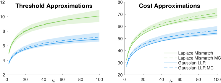
Figure 1: Approximations $\bar{\text{\rm H}}_{2}(\kappa)$ and ${\bar{J}}_{2}(\kappa)$.

figure]f:CostAndThresholdApproximations

3 Reinforcement Learning and QCD

In the few examples we have considered we have found that the approximations in Prop. 2.2 are highly accurate. In non-ideal settings the proposition is valuable in the construction of RL algorithms. We provide algorithms, and full justification in some cases. Algorithm design and analysis is set in the POMDP (Bayesian) setting, with cost criterion (6).

Assumed given is a surrogate belief state: a stochastic process $\{{\cal X}_{k}:k\geq 0\}$, evolving on a closed subset of Euclidean space S, and which is adapted to the observations ${\cal Y}_{k}=\sigma\{Y_{0},\dots,Y_{k}\}$. We do not require that ${\cal X}_{k}$ is in any sense an approximation of an information state. In particular, the numerical experiments largely focus on the CUSUM statistic (3b).

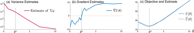
Figure 2: Statistics of the gradient estimate as a function of $\theta$, based on the Actor Critic method: (a) Empirical variance of the gradient estimates. (b) Gradient estimates using $N=10^{4}$ episodes. (c) Objective and its approximation obtained from integrating the gradient estimate.

figure]f:AC

We first consider a version of the actor-critic method, followed by approaches to Q-learning.

Actor-critic method  Assumed given is a collection of randomized stationary policies $\{\widetilde{\upphi}^{\theta}:\theta\in\mathbb{R}^{d}\}$. For each $\theta$ the statistics of the decision rule is defined for each $k$ via

$${\sf P}\{U_{k}=u\mid{\cal Y}_{k};{\cal X}_{k}=x\}=\widetilde{\upphi}^{\theta}(u\mid x)\,,\ \ u\in{\sf U}\,,\ x\in\textsf{S}$$

We fix an initial distribution $\nu$ for the Markov chain $\Psi$, and denote $\mu_{\theta}(\xi,u)=\nu(\xi)\widetilde{\upphi}^{\theta}(u\mid x)$ for $\xi=(\phi;x)\in{\sf X}\times\textsf{S}$ and $u\in{\sf U}$. Our goal is to minimize

$$\Upgamma(\theta)={\sf E}^{\theta}_{\mu_{\theta}}\Big{[}\sum_{k=0}^{\uptau_{\text{\scriptsize\sf s}}}c(\Phi_{k},U_{k})\Big{]}$$ (10)

The subscript indicates that $(\Phi_{0},{\cal X}_{0},U_{0})\sim\mu_{\theta}$, and the superscript “$\theta$” indicates that the policy $\widetilde{\upphi}^{\theta}$ determines the input.

We consider stochastic gradient descent (SGD),

$$\theta_{n+1}=\theta_{n}-\alpha_{n+1}G_{n}{\breve{\nabla}\!}_{\Upgamma}(n)\,,$$ (11)

in which the stepsize $\alpha_{n+1}$ and the matrix gain $G_{n}$ are design choices.

In the actor-critic algorithm the stochastic gradient ${\breve{\nabla}\!}_{\Upgamma}(n)$ is represented in terms of the score function,

$$\Uplambda^{\theta}(x,u)=\nabla_{\theta}\log[\widetilde{\upphi}^{\theta}(u\mid x)]$$ (12)

defined to be zero for any values for which $\widetilde{\upphi}^{\theta}(u\mid x)=0$.

The following result follows from a long history surveyed in the Notes section of [13, Ch. 10]:

Proposition 3.1

Suppose that $\Upgamma$ and $\nabla\Upgamma$ are continuous. Then $\nabla\Upgamma\,(\theta)={\sf E}^{\theta}_{\mu_{\theta}}[{\breve{\nabla}\!}_{\Upgamma}]$, for either of the two options:

$${\breve{\nabla}\!}_{\Upgamma} =\sum_{k=0}^{\uptau_{\text{\scriptsize\sf s}}}c(\Phi_{k},U_{k})S_{k}^{\theta}$$ (13a)

$$\textit{or}\qquad{\breve{\nabla}\!}_{\Upgamma} =\sum_{k=0}^{\uptau_{\text{\scriptsize\sf s}}}Q_{\theta}(\Psi_{k},U_{k})\Uplambda^{\theta}_{k}$$ (13b)

in which $\Uplambda^{\theta}_{k}\mathbin{:=}\Uplambda^{\theta}({\cal X}_{k},U_{k})$, $S_{k}^{\theta}=\Uplambda^{\theta}_{0}+\cdots+\Uplambda^{\theta}_{k}$, and

$$Q_{\theta}(\xi,u)={\sf E}^{\theta}\Big{[}\sum_{k=0}^{\uptau_{\text{\scriptsize\sf s}}}c(\Phi_{k},U_{k})\mid\Psi_{0}=\xi,U_{0}=u\Big{]}$$ (13c)

The two representations for the stochastic gradient (13a) or (13b) lead to two algorithms for SGD without bias. Each of those described here are episodic: data is collected over the period $0\leq k\leq\uptau_{\text{\scriptsize\sf s}}(n)$ with $\theta_{n}$ fixed, and the input defined using $\widetilde{\upphi}^{\theta_{n}}$.

The natural gradient descent algorithm updates the matrix gain via $G_{n}=\widehat{R}_{n}^{-1}$, where $\widehat{R}_{0}>0$ with updates obtained recursively,

$$\widehat{R}_{n} =\widehat{R}_{n-1}+\beta_{n}[-\widehat{R}_{n-1}+R_{n}]\,,\quad n\geq 1\,,$$ (14)

$$R_{n} =\sum_{k=0}^{\uptau_{\text{\scriptsize\sf s}}(n)}\Uplambda^{\theta_{n}}_{k}[\Uplambda^{\theta_{n}}_{k}]^{\intercal}\,,\qquad\Uplambda^{\theta_{n}}_{k}=\Uplambda^{\theta_{n}}({\cal X}_{k},U_{k})$$

with $\beta_{n}\gg\alpha_{n}$ (see [13, Ch. 10]).

The two representations for the gradients prompt two choices for the stochastic gradient. We focus here on the first,

$${\breve{\nabla}\!}_{\Upgamma}(n)=\sum_{k=0}^{\uptau_{\text{\scriptsize\sf s}}(n)}c(\Phi_{k},U_{k})S_{k}^{\theta_{n}}$$

leaving out the extension of the standard algorithm based on TD(1) learning to estimate the Q-function [13, Ch. 10].

The Polyak-Ruppert (PR) estimates are defined by

$$\theta^{\text{\tiny\sf PR}}_{n}=\frac{1}{n}\sum_{i=1}^{n}\theta_{i}\,,\qquad n\geq 1\,.$$ (15)

Its asymptotic covariance is defined as

$$\Sigma^{\text{\tiny\sf PR}}_{\text{\tiny$\Theta$}}=\lim_{n\to\infty}n\,{\sf E}[\tilde{\theta}^{\text{\tiny\sf PR}}_{n}\{\tilde{\theta}^{\text{\tiny\sf PR}}_{n}\}^{\intercal}]$$ (16)

When this exists and is finite, then the estimates achieve the optimal mean-square convergence rate of $O(1/n)$.

The following is a consequence of recent stochastic approximation theory in [2].

Proposition 3.2

Suppose that the assumptions of Prop. 3.1 hold, and in addition (i) $\Upgamma$ is coercive with unique minimum $\theta^{*}$ and $\nabla\Upgamma$ is globally Lipschitz continuous. (ii) $A^{*}\mathbin{:=}\nabla^{2}\Upgamma\,(\theta^{*})$ is Hurwitz, and the steady-state covariance $R^{*}=\hbox{\sf Cov}(\Uplambda^{\theta^{*}})$ is full rank. (iii) The stepsize sequence is $\alpha_{n}=\alpha_{0}n^{-\rho}$ with $1/2<\rho<1$ and $\alpha_{0}>0$.

Then, the SGD algorithm (11) is convergent almost surely and in mean square. The PR-estimates are also convergent in both senses.

The Central Limit Theorem (CLT) holds, as well as the limit (16), in which the asymptotic covariance is $\Sigma^{\text{\tiny\sf PR}}_{\text{\tiny$\Theta$}}=[(R^{*})^{-1}A^{*}]^{\intercal}\Sigma_{\nabla}^{*}(R^{*})^{-1}A^{*}$ with $\Sigma_{\nabla}^{*}$ is the steady-state covariance of (13b) using the policy $\widetilde{\upphi}^{\theta^{*}}$.     $\blacksquare$

Example  Consider the one-dimensional family of policies in which $\theta$ approximates a threshold rule: for a fixed large constant $\upbeta>0$, define $\widetilde{\upphi}^{\theta}(u\mid w)=[1+\exp(\upbeta[w-\theta])]^{-1}\exp(\upbeta u[w-\theta])$, so that the score function is

$$\Uplambda^{\theta}(u\mid w)=-\upbeta u+\upbeta\widetilde{\upphi}^{\theta}(1\mid w)$$

In this scalar example we can adapt the natural gradient actor critic method to estimate $\nabla\Upgamma\,(\theta)$ for any fixed $\theta$.

LABEL:f:AC shows results from a typical experiment using $\upbeta=20$. Details on the simulation environment designed to obtain these approximations are postponed to the Appendix.

Rather than demonstrate results from an application of SGD, the first two plots show estimates of the mean and variance of the random variable in the expectation (13b) for a range of values of $\theta$; the precise means are $\Sigma_{\nabla}\,(\theta)$ and $\nabla\Upgamma\,(\theta)$.

Part (c) shows estimates of the objective function $\Upgamma(\theta)$ obtained via standard Monte-Carlo, and the estimate obtained from gradient estimates via $\widehat{\Upgamma}(\theta)\mathbin{:=}\kappa+\int_{0}^{\theta}\widehat{\nabla}\Upgamma(r)\,dr$. It was found that the plots of $\Upgamma$ and $\widehat{\Upgamma}$ closely match the cost plots obtained from the threshold policies (2) using $\text{\rm H}=\theta$.

Plot (b) indicates good news: in spite of the enormous variance shown in (a), especially high for smaller values of $\theta$, the zero of the gradient estimate $\widehat{\nabla}\Upgamma\,(\theta)$ is very close to the optimal threshold value for CUSUM. However, the massive variance presents a challenge in running the actor-critic algorithm to estimate $\theta^{*}$.

Q-learning  Recall the solution to the POMDP model in which the optimal policy is a function of an information state. Consider the canonical example in which this is the belief state (the sequence of conditional distributions), and assume that the underlying Markov chain $\Phi$ evolves on a finite set so that the simplex ${\cal S}$ is finite-dimensional.

The Q-function $Q^{*}\colon{\cal S}\times{\sf U}\to\mathbb{R}$ is the optimal value function associated with the objective (4). To place the equations in standard form denote $c(x,u)=(1-u)c_{\circ}(x)+uc_{\bullet}(x)$ for $x\in{\sf X}$ and $u\in\{0,1\}$ (recall (4)). For any $\beta,u$ denote ${\cal C}(\beta,u)=\sum_{x}\beta(x)c(x,u)$.

The value $Q^{*}(\beta,u)$ is defined to be the minimum of $\sum_{\phi}\beta(\phi)J(\phi,U_{0}^{\infty})$ over all admissible $U_{1}^{\infty}$, subject to $(\Uppi_{0},U_{0})=(\beta,u)$. It satisfies the dynamic programming (DP) equation,

$$Q^{*}(\beta,u)={\cal C}(\beta,u)+{\sf E}[\underline{Q}^{*}(\Uppi_{k+1})\mid\Uppi_{k}=\beta,U_{k}=u]$$

with $\underline{H}(\beta)=\min\{H(\beta,0),H(\beta,1)\}$ for any function $H\colon{\cal S}\times{\sf U}\to\mathbb{R}$.

Q-learning algorithms are based on the characterization: ${\sf E}\bigl{[}\mathcal{D}^{*}_{k+1}\mid{\cal Y}_{k}\big{]}=0$ or each $k$ and any adapted input, with $\mathcal{D}^{*}_{k+1}=-Q^{*}(\Uppi_{k},U_{k})+c_{k}+\underline{Q}^{*}(\Uppi_{k+1})$. with $c_{k}=(1-U_{k})\hbox{\large\bf 1}\{\uptau_{\text{\scriptsize\sf a}}<k\}+\kappa\,U_{k}(\uptau_{\text{\scriptsize\sf a}}-k)_{+}$.

This motivates typical Q-learning algorithms.

Given a parameterized family of real-valued functions $\{Q^{\theta}:\theta\in\mathbb{R}^{d}\}$ on $\textsf{S}\times{\sf U}$, the goal is to solve the projected Bellman equation: ${\widebar{f}}(\theta^{*})=0$ with

$${\widebar{f}}(\theta)\mathbin{:=}{\sf E}\bigl{[}\{-Q^{\theta}({\cal X}_{k},U_{k})+c_{k}+\underline{Q}^{\theta}({\cal X}_{k+1})\}\zeta_{k}\bigr{]}$$ (17)

where $\{\zeta_{k}\}$ is a $d$-dimensional stochastic process adapted to the observations.

It is typical to take $\zeta_{k}=\nabla_{\theta}Q^{\theta}({\cal X}_{k},U_{k})\big{|}_{\theta_{k}}$, with $\theta_{k}$ the estimate at iteration $k$. Theory to-date is largely restricted to a linear function class in which $Q^{\theta}=\theta^{\intercal}\psi$ with $\psi\colon\textsf{S}\times{\sf U}\to\mathbb{R}^{d}$, and in this case $\zeta_{k}=\psi({\cal X}_{k},U_{k})$.

Data required in an algorithm is based on successive runs up to time $\uptau_{\text{\scriptsize\sf s}}(n)$ for $n\geq 1$, which results in the observations $\{{\cal X}_{k}^{n},{\cal X}_{k+1}^{n},U_{k}^{n},c(\Phi_{k}^{n},U_{k}^{n})\}$ for $0\leq k<\uptau_{\text{\scriptsize\sf s}}(n)$. We suppress dependency on $n$ by stringing data together, so that for example

$$U_{k}\mathbin{:=}U_{k-\uptau_{\text{\scriptsize\sf s}}(n-1)}^{n}\ \ \textit{for $\uptau_{\text{\scriptsize\sf s}}(n-1)\leq k<\uptau_{\text{\scriptsize\sf s}}(n)$ and $n\geq 1$,}$$

with $\uptau_{\text{\scriptsize\sf s}}(0)\mathbin{:=}0$.

A version of Q-learning is expressed as the recursion

$$\theta_{k+1} =\theta_{k}+\alpha_{k+1}G_{k}\zeta_{k}\mathcal{D}_{k+1}\,,\qquad\qquad k\geq 0$$ (18a)

$$\mathcal{D}_{k+1} =-Q^{\theta_{k}}({\cal X}_{k},U_{k})+c_{k}+\underline{Q}^{\theta_{k}}({\cal X}_{k+1})$$ (18b)

where the matrix gain sequence $\{G_{k}\}$ is a design choice; Zap Q-learning is in some sense optimal [13]; This matrix gain was used in [3] for applications to optimal stopping.

We cannot apply [3], based on the elegant algorithm of [21], since the resulting policy will depend on the cost $\{c(\Phi_{k},U_{k})\}$ (assumed observed in this prior work).

While there is great empirical success in the history of Q-learning, to-date we only have general conditions for stability of the algorithm, and existence of a solution to the projected Bellman equation [14]. Most crucial is the requirement that the input used for training is an $\varepsilon$-greedy policy (or a smoothed variant). It is shown that, subject to a mild full rank condition for $\psi$, that for sufficiently small $\varepsilon>0$ the algorithm (18a) is stable in the sense of ultimate boundedness, and there exists at least one solution $\theta^{*}\in\mathbb{R}^{d}$ to the projected Bellman equation ${\widebar{f}}(\theta^{*})=0$. Convergence remains a topic of research.

Stability of Zap Q-learning with an oblivious policy (independent of parameter) is virtually universal [4], but this paper makes no claims of existence of $\theta^{*}$ in this setting. It is very likely that the main result of [4] can be extended to $\varepsilon$-greedy policies.

4 Numerical Results

The results surveyed here consider conditionally Gaussian observations, $X^{0}_{k}\sim{\cal{N}}(0,\sigma^{2})=\breve{f}^{0}$ and $X^{1}_{k}\sim{\cal{N}}(\mu_{1},\sigma^{2})=\breve{f}^{1}$ with $\mu_{1}=0.5$ and $\sigma=1$. We present findings using $\widehat{L}=\log(\breve{f}^{1}/\breve{f}^{0})$ for three choices of $\{\breve{f}^{0},\breve{f}^{1}\}$:

Case 1: The ideal Gaussian case, in which $\breve{f}^{0}$ and $\breve{f}^{1}$ are the true densities.
Case 2: $\breve{f}^{0}$ is Laplace$(0,b)$ and $\breve{f}^{1}$ Laplace$(\mu_{1},b)$ with $\mu_{1}=0.5$ and $b=\sqrt{\sigma/2}$ (matching second order statistics).
Case 3: $\breve{f}^{0}$ is Cauchy$(0,\gamma)$ and $\breve{f}^{1}$ Cauchy$(x_{1},\gamma)$ with $x_{1}=0.5$ and $\gamma$ chosen so that the Gaussian and Cauchy cdfs evaluated at $\sigma=1$ are equal.

Ground truth  The observations were specified by Shiryaev’s conditional i.i.d. model (5) and with $\uptau_{\text{\scriptsize\sf a}}\sim\text{Geometric}($0.02$)$, so that we have in hand the optimal policy for comparison.

The policies of interest will be functions of the the RRW (3b). The term optimal CUSUM refers to the test obtained with threshold $\text{\rm H}_{\textsf{\tiny CU}}(\kappa)$ obtained via

$$\text{\rm H}_{\textsf{\tiny CU}}(\kappa)=\mathop{\rm arg\,min}_{\text{\rm H}\geq 0}\{\kappa{\sf MDE}(\text{\rm H})+{\sf MDD}(\text{\rm H})\}$$ (19)

where ${\sf MDE}(\text{\rm H})$ and ${\sf MDD}(\text{\rm H})$ are obtained using CUSUM with threshold $\text{\rm H}\geq 0$. These thresholds and those for Shiryaev’s optimal test were estimated via Monte-Carlo—details are postponed to the Appendix.

We find that optimal CUSUM is nearly optimal, even in non-asymptotic settings, for the model considered (see LABEL:f:Performance and discussion below).

4.1 Cost approximation

Approximations based on the analysis in Section 2.2 were obtained for $\varrho_{\text{\scriptsize\sf a}}=0.02$ (recall (8)).

For the ideal case $\widehat{L}$ is the true LLR with respect to the observations, so that $F(x)=\widehat{L}(x)=\mu_{1}x-\mu_{1}^{2}/2$. The log moment generating function is $\Lambda_{0}(\theta)=m_{1}\theta(\theta-1)$. The equation $\varrho_{\text{\scriptsize\sf a}}=\Lambda_{0}(\theta^{*}_{+})$ is easily inverted to obtain $\theta^{*}_{+}>0$. For the mismatched cases $\theta^{*}_{+}$ was approximated through simulation: see LABEL:f:Lam0GaussLaplace.

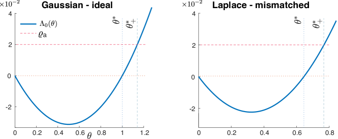
Figure 3: $\Lambda_{0}(\theta)$ for ideal Gaussian and Laplace mismatched detector

figure]f:Lam0GaussLaplace

For each choice of $F$ we obtained threshold and cost approximations ${\bar{H}}_{\infty}^{*}(\kappa)$ and ${\bar{J}}_{\infty}^{*}(\kappa)$ as defined in Section 2. In the plots that follow, approximations are shifted:

$$\bar{\text{\rm H}}_{2}(\kappa) ={\bar{H}}_{\infty}^{*}(\kappa)-{\bar{H}}_{\infty}^{*}(2)+{\bar{H}}^{*}_{\tiny{\sf true}}(2)$$

$${\bar{J}}_{2}(\kappa) ={\bar{J}}_{\infty}^{*}(\kappa)-{\bar{J}}_{\infty}^{*}(2)+{\bar{J}}_{\tiny{\sf true}}(2)$$

where the true values are based on results for $\kappa=2$, the smallest in our selected range.

The final approximations are shown in LABEL:f:CostAndThresholdApproximations, compared to ground truth estimates with $1\sigma$ confidence intervals. We find that the approximations are remarkably accurate. Compared to the ideal, the results predict a 25% increase in cost for Case 2 and a 43% increase for Case 3 at the highest value in our experimental range $\kappa=100$.

4.2 Q-learning

The remainder of this section presents the design and evaluation of Q-learning for our Bayesian QCD problem.

Basis selection  Bases considered for Q-learning took the form $\psi(x,u)=(1-u)\psi^{0}(x)+u\psi^{1}(x)$. The numerical results shown in the following used

$$\psi^{0}(x)=[x;q(x);0;0;0]$$

$$\psi^{1}(x)=[0;0;1;x;q(x))]$$ (20)

with $q(x)=x\exp(-x/b_{q})$ for a choice of constant $b_{q}$.

This basis was designed based on preliminary experiments with a particular choice of binning: $\psi_{i}(x,u)=\hbox{\large\bf 1}\{x\in S_{k_{i}},u=u^{i}\}$ for a collection of intervals $\{S_{j}\}$ and input values $\{u^{j}\}$. Further details are provided below.

Exploration.  Recent theory recalled in Section 3 shows that exploration implies stability of the algorithm under mild assumptions on the basis and the oblivious policy. The value of $\varepsilon$ was taken to be time varying, with a typical choice illustrated in LABEL:f:TypicalTrajectories: $\varepsilon_{n}=\max\{\varepsilon_{f},\varepsilon_{0}+(1-n/n_{0})(\varepsilon_{f}-\varepsilon_{0})\}$, defined so that $\varepsilon_{n}=\varepsilon_{f}<\varepsilon_{0}$ for $n\geq n_{0}$. The values $\varepsilon_{0}=0.75$ and $\varepsilon_{f}=0.1$ worked well with Zap Q-learning, whereas standard scalar gain Q-learning required $\varepsilon_{f}\ll 0.1$ for stability.

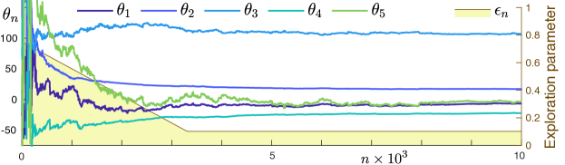
Figure 4: Parameter estimates using a decaying exploration schedule.

figure]f:TypicalTrajectories

Exploration was designed to depend on $\kappa$ based on properties of the CUSUM statistic (3b). It is known that a threshold $\text{\rm H}^{*}=\left|\log\upsilon\right|$ is optimal in the minimax setting where $\upsilon$ is a constraint on false alarm rate (${\sf FAR}$) [23]. In our Bayesian setting, we show that a similar logarithmic relationship exists between $\text{\rm H}^{*}$ and $\kappa$ in Prop. 2.2. We leveraged this analysis for the oblivious policy, which is described as follows: at the start of episode $i$, a threshold $\text{\rm H}^{\varepsilon,i}(\kappa)$ was drawn uniformly at random from interval $[a_{\kappa},b_{\kappa}]$, where $a_{\kappa}=\eta\log\left(\kappa+1-\kappa_{\min}\right)$ and $b_{\kappa}=a_{\kappa}+\delta$. Parameters $\delta$ and $\eta$ determine the width and rate of increase of $[a_{\kappa},b_{\kappa}]$ as $\kappa$ increases. $\kappa_{\min}$ is the smallest multiplier in our range. Then, $U_{n}=\hbox{\large\bf 1}\{{\cal X}_{n}\geq\text{\rm H}^{\kappa,i}\}$ for each $n$ in this episode. This ensured significant exploration, even when considering high dimensional bases obtained through binning.

Numerical experiments  Recall that in Q-learning any parameter $\theta\in\mathbb{R}^{d}$ defines a policy, $\upphi^{\theta}(x)=\mathop{\rm arg\,min}_{u}Q^{\theta}(x,u)$ for $x\in\mathbb{R}_{+}$. In the applications considered here this becomes

$$\upphi^{\theta}(x)=\hbox{\large\bf 1}\{Q^{\theta}(x,0)\geq Q^{\theta}(x,1)\}\,,\qquad x\in\mathbb{R}_{+}\,.$$ (21)

In every successful application of Q-learning it was found that this policy had a threshold form

$$\upphi^{\theta}(x)=\hbox{\large\bf 1}\{x\geq\text{\rm H}^{\theta}\}\,,\quad\text{\rm H}^{\theta}>0$$ (22)

Algorithm performance is investigated in the remainder of this section. For each algorithm, PR-averaging is used to define the final estimate ${\hat{\theta}}$, and from this a final policy $\widehat{\upphi}\mathbin{:=}\upphi^{{\hat{\theta}}}$ whose performance is compared to the optimal.

Recall that initial experiments involved a choice of binning, resulting in $d=2(d_{0}-1)$, with $d_{0}$ the number of bins. Given the structure of the problem it was decided that the bin boundaries should be spaced logarithmically. We assigned wider bins to capture larger values of $x$, which are expected to occur less frequently given an adequate threshold policy of the form (22). However, binning proved insufficient for obtaining thresholds close to optimal over all $\kappa$, due in part to a tradeoff between the choice of bin spacing and granularity of the linear interpolation required to obtain $\text{\rm H}^{\theta}$.

This shortcoming is illustrated in Fig. 5, where bin spacing influences the intersection $Q^{\theta}(w,0)=Q^{\theta}(w,1)$ and the policy (recall (21)). This inspired the “smooth” basis defined in (20) for which we observed two advantages compared to binning: 1/ consistent improvement of $\text{\rm H}^{\theta}$ compared to optimal over all $\kappa$, and 2/ reduced computation time.

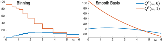
Figure 5: Insights from binning led to the basis in (20)

.

Histograms were generated to evaluate the variance of the parameter estimates. Let $\upxi=\upxi(N)\geq N$ denote the total number of samples $({\cal X}_{k},U_{k})$ collected over $N$ episodes, so that ${\hat{\theta}}=\theta^{\text{\tiny\sf PR}}_{\upxi}$ is the final estimate. The batch means method was used to estimate the asymptotic covariance of the error $\tilde{\theta}^{\text{\tiny\sf PR}}_{\upxi}\mathbin{:=}\theta^{\text{\tiny\sf PR}}_{\upxi}-\theta^{*}$, defined on scaling, taking expectations, and letting $N\to\infty$:

$$\Sigma^{\text{\tiny\sf PR}}_{\text{\tiny$\Theta$}}=\lim_{N\to\infty}{\sf E}[\upxi\,\tilde{\theta}^{\text{\tiny\sf PR}}_{\upxi}\{\tilde{\theta}^{\text{\tiny\sf PR}}_{\upxi}\}^{\intercal}]$$

This was estimated by performing $M>1$ independent runs to obtain $\{\theta^{\text{\tiny\sf PR}}_{\upxi^{i}},\upxi^{i}:1\leq i\leq M\}$, and a histogram of $Z^{i}=\sqrt{\upxi^{i}}[\theta^{\text{\tiny\sf PR}}_{\upxi^{i}}-\bar{\theta}^{\text{\tiny\sf PR}}]$ to estimate the variance of each entry. An example is shown in LABEL:f:Hists for the case $\kappa=27$, using $M=400$ and three different values of $N$. Only the fourth component of the five dimensional histogram is shown—the others are similar.

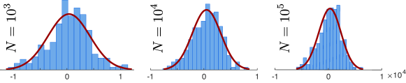
Figure 6: Histograms of $\{Z^{i}_{1}:1\leq i\leq M\}$ for three values of $N$.

figure]f:Hists

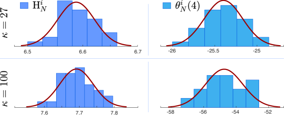
Figure 7: Histograms of $\{\text{\rm H}_{N}^{i},\theta_{N}^{i}(4):1\leq i\leq M\}$ for $N=10^{6}$

figure]f:HistsPar+Thresh27+100

What is crucial here is that the empirical variance is nearly identical for the last two values of $N$ chosen. This is an example of how the CLT can be used to estimate required run lengths by first conducting a large number of independent experiments with a relatively short run length—in this example, $N=10^{4}$ provides a reasonable estimate of the variance of $Z^{i}=\sqrt{\upxi^{i}}[\theta^{\text{\tiny\sf PR}}_{\upxi^{i}}-\bar{\theta}^{\text{\tiny\sf PR}}]$ for each $i$ and $N\gg 10^{4}$.

We further observed a relative sensitivity between thresholds obtained through Q-learning and parameter estimates: thresholds $\text{\rm H}_{N}^{i}$ consistently yielded smaller empirical variance than $\theta_{N}^{i}$ for all $\kappa$. Example histograms showing the fourth parameter $\theta_{N}^{i}(4)$ are included in LABEL:f:HistsPar+Thresh27+100 for $M=30$ and $N=10^{6}$.

LABEL:f:Performance shows the average cost of the policy $\widehat{\upphi}$ for the ideal Gaussian case, along with what is obtained with the optimal test and optimal CUSUM with confidence intervals of $\sigma/3$ standard deviation. As $\kappa$ increases, Q-learning quickly yields average cost close to optimal.

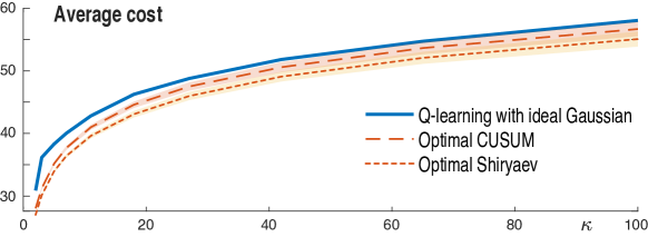
Figure 8: Average cost comparisons.

figure]f:Performance

Mismatched cases.  We consider a setting where the goal is achieving the best performance for the ideal Gaussian case, while evaluating performance of the mismatched cases in parallel. The surrogate information state $\{{\cal X}_{n}\}$ differs between each case based on the three respective log-likelihood ratios, shown in LABEL:f:3LLRs. Laplace and Cauchy are very far from the ideal.

Clues for tuning exploration parameters values $\eta$ and $\delta$ came from asymptotic analysis of our eagerness and delay costs. The interval $[a_{\kappa},b_{\kappa}]$ was designed such that threshold approximations $\bar{\text{\rm H}}_{2}(\kappa)$ follow uniform interval mean ${\mathchoice{\genfrac{}{}{}{1}{1}{2}}{\genfrac{}{}{}{1}{1}{2}}{\genfrac{}{}{}{3}{1}{2}}{\genfrac{}{}{}{3}{1}{2}}}(a_{\kappa}+b_{\kappa})$ for all $\kappa$. Initial experiments sought to produce random thresholds $\text{\rm H}^{\varepsilon}(\kappa)$ encouraging an equal balance of eagerness and delay throughout each episode, but it was later found that a greater ratio of eagerness yielded $\text{\rm H}^{\theta}$ closer optimal.

A choice of large $\delta$ was tried universally for each case, leading to $\text{\rm H}^{\theta}$ far greater than their respective CUSUM optimal threshold. Resulting average costs were highest for Case 3, followed by Case 2 and Case 1 for all $\kappa$. This was consistent with cost approximations ${\bar{J}}_{2}(\kappa)$ for each case. Another metric for success is that the shape of the average cost curve obtained through Q-learning resembles its optimal counterpart. This indicates flexibility in learning near-optimal policies of the form (22) over a wide range of $\kappa$, as shown in LABEL:f:Performance for Case 1. For each case with was not yet observed until $\delta$ was lowered, narrowing $[a_{\kappa},b_{\kappa}]$. This lowered the average cost across all three cases, with Case 1 improving the most. As the exploration strategy improved to produce near-optimal average cost for Case 1, we obtain $\text{\rm H}^{\theta}=\infty$ for Cases 2 and 3 for $\kappa>11$, where $Q^{\theta}(w,1)>Q^{\theta}(w,0)$ for all $w$. These findings suggest a tight link between our choice of exploration and the asymptotic statistics for our Bayesian QCD problem–as Q-learning for the ideal case improves, the mismatched cases fail for higher $\kappa$.

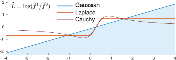
Figure 9: Three LLRs

figure]f:3LLRs

Alternatives to Zap.  Associated with any stochastic approximation algorithm such as the Q-learning algorithm (18a) is an ODE ${\mathchoice{\genfrac{}{}{}{1}{d}{dt}}{\genfrac{}{}{}{1}{d}{dt}}{\genfrac{}{}{}{3}{d}{dt}}{\genfrac{}{}{}{3}{d}{dt}}}\upvartheta=G(\theta){\widebar{f}}(\upvartheta)$, in which ${\widebar{f}}$ is the mean increment of the recursion without matrix gain. For Zap Q-learning we have $G=-{\bar{A}}^{-1}$, with ${\bar{A}}(\theta)\mathbin{:=}-\partial_{\theta}{\widebar{f}}\,(\theta)$. To see if the algorithm is convergent without a matrix gain we examine the linearization to see if the ODE is locally asymptotically stable. In all cases it was not: some eigenvalues of ${\bar{A}}(\theta^{*})$ lay in the strict right half plane.

Theory in [14] predicts stability without a matrix gain, so further testing was performed to investigate the behavior with a scalar gain, and also the popular choice $G=R^{-1}$ in which $R(\theta)={\sf E}[\psi_{k}\psi_{k}^{\intercal}]$ (expectation in steady-state with fixed policy $\upphi^{\theta}$). Estimates are obtained precisely through the recursion (14), with $\Uplambda^{\theta_{n}}_{k}$ replaced by $\psi_{k}=\psi({\cal X}_{k};U_{k})$. The scalar gain algorithm used $g_{n}=1/\hbox{\rm trace\,}(R_{n})$, so that $G_{n}=g_{n}I$ in (18a).

The parameter estimates were unbounded using the exploration schedule with $\varepsilon_{f}=0.1$. Theory in [14] predicts stability with a sufficiently small value, and indeed we observed convergence with $\varepsilon_{f}=0.001$.

We consistently find that the policy is of the threshold form (22) but with $\text{\rm H}^{\theta}$ smaller than optimal, leading to high eagerness cost. We further observed a lack of sensitivity between $\text{\rm H}^{\theta}$ and $\kappa$ compared to Zap Q-learning. This resulted in worsening average cost for higher $\kappa$, which is the regime of greatest interest in typical applications. Very similar results are obtained using $G_{n}=R_{n}^{-1}$.

In all Zap Q-learning applications, ${\bar{A}}(\theta^{*})$ was non-Hurwitz even for exploration schedules with values as small as $\varepsilon_{f}=10^{-4}$. This suggests there are solutions to the projected Bellman equation using Zap Q-learning that could never be found using standard scalar gain algorithms.

5 Conclusions

The theory and numerical results in this paper motivate many directions for future research. For actor critic methods it is crucial to find ways to reduce variance, perhaps through other approaches to gradient free optimization. Within the ideal setting of Section 4, we present results closely matching the performance of optimal CUSUM using Q-learning.

This work is intended to be a starting point for consideration of highly non-ideal settings faced in practice. In applications of interest to us there may be well understood behavior before a change (which might represent a fault in a transmission line, or a computer attack). We cannot expect to have a full understanding of post-change behavior. The choice of surrogate information state must be reconsidered in these settings. We must take into account correlation of observations before a change has occurred.

Prior work in [11] provides a roadmap for analysis of non-stationary post-change behavior. Design of new architectures, that may be trained using techniques surveyed in this paper, might be inspired by the rich literature on composite hypothesis testing (see [22, 7] and the references therein).

Appendix A Appendix

Below we include proofs the asymptotic analysis of our Bayesian QCD problem, followed by simulation details for the QCD and RL experiments.

A.1 Asymptotic statistics for Bayesian QCD

Most of this subsection is devoted to a proof of Prop. 2.2. We begin with the simpler,

Proof of Lemma 2.1  Let $M$ denote the non-negative sub-matrix $M_{i,j}=P_{i,j}\hbox{\large\bf 1}\{j\in{\sf X}_{1}\}$, defined only for $i,j\in{\sf X}_{1}$. The assumptions on $\uptau_{\text{\scriptsize\sf a}}$ imply irreducibility in a weak sense: for some $i_{0}\in{\sf X}_{1}$ we have $\sum_{k=1}^{n}M^{k}_{i,i_{0}}>0$ for all $i\in{\sf X}_{1}$ and all $n\geq 1$ sufficiently large. Let $(\lambda,v)$ denote the Perron Frobenious eigenvalue/eigenvector [16]. The eigenvalue $\lambda>0$ is maximal, the vector $v$ entries that are strictly positive, and $\sum_{j\in{\sf X}_{1}}M_{i,j}v_{j}=\lambda v_{i}$ for $i\in{\sf X}_{1}$.

The twisted transition matrix has entries ${\check{P}}_{i,j}=\lambda^{-1}v_{i}^{-1}M_{i,j}v_{j}:i,j\in{\sf X}_{1}$; the finiteness assumption for ${\sf X}_{1}$ is imposed to ensure that ${\check{P}}$ defines a Markov chain on ${\sf X}_{1}$ that is positive recurrent. Let $\check{\pi}$ denote its unique invariant pmf.

Positive recurrence implies something far stronger than the limit claimed in the proposition: We have for each $i,j\in{\sf X}_{1}$,

$$\check{\pi}(j)=\lim_{n\to\infty}{\check{P}}^{n}_{i,j}=v_{i}^{-1}v_{j}\lim_{n\to\infty}\lambda^{-n}M_{i,j}^{n}$$

where convergence holds at a geometric rate. Multiplying each side by $1/v_{j}$ and summing over $j$ gives

$$\check{\pi}(1/v)=v_{i}^{-1}\lim_{n\to\infty}\lambda^{-n}{\sf P}\{\uptau_{\text{\scriptsize\sf a}}>n\}$$

where the probability is conditional on $\Phi_{0}=i$. Again, the rate of convergence is geometric, so for each $i$ there is a geometrically decaying sequence $\{\varepsilon_{n}(i)\}$ such that

$${\sf P}\{\uptau_{\text{\scriptsize\sf a}}\geq n+1\}=[\check{\pi}(1/v)+\varepsilon_{n}(i)]\lambda^{n}v_{i}$$

Consequently, (8) holds with $\varrho_{\text{\scriptsize\sf a}}=-\log(\lambda)$.     $\blacksquare$

The bulk of the proof of Prop. 2.2 is based on approximating the cost of eagerness.

For each $i=0,1$, the log moment generating function for $f_{i}$ is denoted $\Lambda_{i}(\theta)=\log\int\exp(\theta F(y))f_{i}(y)\,dy$, $\theta\in\mathbb{R}$, with convex dual $I_{i}(m)=\sup_{\theta}\{m\theta-\Lambda_{i}(\theta)\}$, $m\in\mathbb{R}$. Each is a convex, possibly extended-valued function on $\mathbb{R}$.

Most significant in this analysis is the case $i=0$:

Lemma A.1

The log moment generating function $\Lambda_{0}$ is convex. Provided it is finite in a neighborhood of the origin, it satisfies $\Lambda_{0}^{\prime}(0)=m_{0}<0$ and $\Lambda_{0}^{\prime\prime}(0)=\sigma^{2}_{0}$, the variance of $F(Y)$ under $f_{0}$. If there is a second root $\theta^{*}>0$, then $\Lambda_{0}(\theta)<0$ on the open interval $(0,\theta^{*})$.

The special case $F=\log(f_{1}/f_{0})$ gives $\Lambda_{0}^{\prime}(0)=m_{0}=-D(f_{0}\|f_{1})$; $\theta^{*}=1$, and $\Lambda_{0}^{\prime}(\theta^{*})=m_{1}=D(f_{1}\|f_{0})$.     $\blacksquare$

For any $\tau\geq 0$, the approximation of ${\sf E}[(\uptau_{\text{\scriptsize\sf s}}-\uptau_{\text{\scriptsize\sf a}})_{-}\mid\uptau_{\text{\scriptsize\sf a}}=\tau]$ is made possible through the rich literature on rare events for RRWs, e.g. [1, 6]: It is known that the most likely path for the random walk to hit a high level is piecewise linear, with identifiable slope equal to $m^{*}=\Lambda_{0}^{\prime}(\theta^{*})$. Since $\theta^{*}$ is a second root of $\Lambda_{0}$ it easily follows that $I_{0}(m^{*})=m^{*}\theta^{*}$.

To make precise the term “likely path” we perform the standard temporal and spatial scaling. Suppose that $\{{\cal X}_{n}\}$ is defined as the RRW (3b) initialized with ${\cal X}_{0}=0$, and $\uptau_{\text{\scriptsize\sf a}}=\infty$ so that $L_{n}=F(X_{k}^{0})$ for all $k$. For a given threshold $\text{\rm H}>0$ denote by $\{x^{\text{\sf\tiny(H)}}_{t}:t\geq 0\}$ the continuous function defined by $x^{\text{\sf\tiny(H)}}_{t}=\text{\rm H}^{-1}{\cal X}_{k}$ for $t=k/\text{\rm H}$, and by piecewise linear interpolation for all other $t\geq 0$. When $\uptau_{\text{\scriptsize\sf s}}$ is defined using threshold H, then $\uptau_{\text{\scriptsize\sf s}}\leq T\text{\rm H}$ if and only if $x^{\text{\sf\tiny(H)}}_{t}\geq 1$ for some $t\leq T$.

For any $T>0$, denote $m(T)=\max(1/T,m^{*})$ and $e_{0}(T)=I_{0}(m(T))/m(T)$.

Lemma A.2

Under the assumptions of Prop. 2.2 we have

$$\lim_{\text{\rm H}\to\infty}\frac{1}{\text{\rm H}}\log{\sf P}\Bigl{\{}\sup_{0\leq t\leq T}x^{\text{\sf\tiny(H)}}_{t}\geq 1\Bigr{\}}=-e_{0}(T)\,,\ \ T>0\,.$$

The exponent $e_{0}(T)$ is minimized when $T\geq 1/m^{*}$.

Proof  This is explained in [6, Section 6.4] through the contraction principle of large deviations theory. A rate function on sample paths is defined by $I(m,x)=I_{0}(m)$ for $x>0$ and $I(m,x)=0$ otherwise; the contraction principle gives

$$\lim_{\text{\rm H}\to\infty}\frac{1}{\text{\rm H}}\log{\sf P}\Bigl{\{}\sup_{0\leq t\leq T}x^{\text{\sf\tiny(H)}}_{t}\geq 1\Bigr{\}}=-\inf\int_{0}^{T}I(\dot{x}_{t},x_{t})\,dt$$

where the infimum is over all absolutely continuous paths $\{x_{t}:0\leq t\leq T\}$ satisfying $x_{0}=0$ and $\max_{0\leq t\leq T}x_{t}\geq 1$. An optimal solution is known to be piecewise linear, with a single value $t_{1}\in(0,T]$ at which $x^{*}_{t_{1}}=1$. Two possible cases are illustrated in LABEL:f:MostLikelyPaths.

The figure on the left hand side illustrates $x^{*}$ when $T>1/m^{*}$. In this case the optimal solution is not unique: for any value $1/m^{*}\leq t_{1}\leq T$, an optimal solution is obtained with $x^{*}_{t}=0$ for $0\leq t\leq t_{0}=t_{1}-1/m^{*}$, ${\mathchoice{\genfrac{}{}{}{1}{d}{dt}}{\genfrac{}{}{}{1}{d}{dt}}{\genfrac{}{}{}{3}{d}{dt}}{\genfrac{}{}{}{3}{d}{dt}}}x_{t}^{*}=m^{*}>0$ for $t_{0}<t<t_{1}$, and $x_{t}^{*}=\max(0,1+m_{0}(t-t_{1})$ for $t\geq t_{1}$.

If $0<T\leq 1/m^{*}$ then $t_{0}=0$ and $t_{1}=T$ so that $x_{t}^{*}=\max(0,\min(t/T,1+(t-T)m_{0}))$, as shown on the right hand side of the figure.

In either case we have by the definitions ${\mathchoice{\genfrac{}{}{}{1}{d}{dt}}{\genfrac{}{}{}{1}{d}{dt}}{\genfrac{}{}{}{3}{d}{dt}}{\genfrac{}{}{}{3}{d}{dt}}}x_{t}^{*}=m(T)$ for $t_{0}<t<t_{1}=t_{0}+1/m(T)$, and

$$\int_{0}^{T}I(\dot{x}_{t}^{*},x_{t}^{*})\,dt=[t_{1}-t_{0}]I_{0}(m(T))=\frac{1}{m(T)}I_{0}(m(T))$$

$\blacksquare$

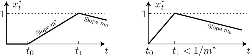
Figure 10: Most likely paths: the path shown on the left is far more probable than the one shown on the right.

figure]f:MostLikelyPaths

Proof of Prop. 2.2  To approximate the cost of eagerness we require approximations of ${\sf P}\{\uptau_{\text{\scriptsize\sf s}}\leq n\mid\uptau_{\text{\scriptsize\sf a}}=n+k\}$ for any $n$ and all $k\geq 1$. Since $\uptau_{\text{\scriptsize\sf a}}$ is independent of $\{X_{k}^{0}\}$, it suffices to restrict to the setting of Lemma A.2 in which $\uptau_{\text{\scriptsize\sf a}}=\infty$. In particular, for any $n\geq 1$ let $T_{n}=n/\text{\rm H}$. Independence combined with Lemma A.2 gives, for any $k\geq 1$,

$${\sf P}\{\uptau_{\text{\scriptsize\sf s}}\leq n \mid\uptau_{\text{\scriptsize\sf a}}=n+k\}={\sf P}\{\max_{0\leq t\leq T_{n}}x^{\text{\sf\tiny(H)}}_{t}\geq 1\}$$

$$=\exp\big{(}-\text{\rm H}[e_{0}(T_{n})+\varepsilon_{\text{\scriptsize\sf s}}(\text{\rm H},T_{n})]\big{)}$$

in which $\varepsilon_{\text{\scriptsize\sf s}}(\text{\rm H},T)\to 0$ as $\text{\rm H}\to\infty$, uniformly for $T$ in compact sets of $(0,\infty)$.

The expected eagerness is thus

$${\sf E}[(\uptau_{\text{\scriptsize\sf s}}-\uptau_{\text{\scriptsize\sf a}})_{-}] =\sum_{\tau=1}^{\infty}\sum_{n=0}^{\tau-1}{\sf P}\{\uptau_{\text{\scriptsize\sf s}}\leq n\mid\uptau_{\text{\scriptsize\sf a}}=\tau\}{\sf P}\{\uptau_{\text{\scriptsize\sf a}}=\tau\}$$

$$=\sum_{n=0}^{\infty}{\sf P}\{\max_{0\leq t\leq T_{n}}x^{\text{\sf\tiny(H)}}_{t}\geq 1\}{\sf P}\{\uptau_{\text{\scriptsize\sf a}}>n\}$$

We next write ${\sf P}\{\uptau_{\text{\scriptsize\sf a}}>n\}=\exp(-n[\varrho_{\text{\scriptsize\sf a}}+\varepsilon_{\text{\scriptsize\sf c}}(n)])$ where $\varepsilon_{\text{\scriptsize\sf c}}(n)\to 0$ as $n\to\infty$. Combining these approximations, we write the expected eagerness as

$$\sum_{n=0}^{\infty}\exp\bigl{(}-\text{\rm H}[e_{0}(T_{n})+\varepsilon_{\text{\scriptsize\sf s}}(\text{\rm H},T_{n})]-n[\varrho_{\text{\scriptsize\sf a}}+\varepsilon_{\text{\scriptsize\sf c}}(n)]\bigr{)}$$

The dominant term in the exponent is $\text{\rm H}e_{0}(T_{n})+n\varrho_{\text{\scriptsize\sf a}}=\text{\rm H}[e_{0}(T_{n})+T_{n}\varrho_{\text{\scriptsize\sf a}}]$, which is affine with slope $\varrho_{\text{\scriptsize\sf a}}$ for $T_{n}\geq 1/m^{*}$. This is illustrated in LABEL:f:EagerExp in which $n^{*}_{0}=\lfloor\text{\rm H}/m^{*}\rfloor$ with $m^{*}=\Lambda_{0}^{\prime}(\theta^{*})$, and we will see that the minimizer is approximately $n^{*}=\lfloor\text{\rm H}/m^{*}_{+}\rfloor$ with $m^{*}_{+}=\Lambda_{0}^{\prime}(\theta^{*}_{+})$.

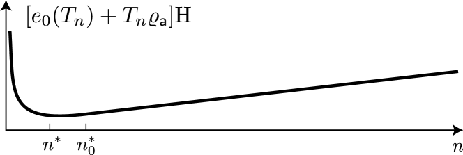
Figure 11: Negative logarithm of eagerness cost approximation.

figure]f:EagerExp

To minimize over $T_{n}$, we consider $m=\max(m^{*},1/T_{n})$ as a variable, so that $e_{0}(T_{n})+T_{n}\varrho_{\text{\scriptsize\sf a}}=[I_{0}(m)+\varrho_{\text{\scriptsize\sf a}}]/m$ for $m\geq m^{*}$. This is a convex function of $m$, whose unique minimum is found by computing the stationary point: $0=[mI_{0}^{\prime}(m)-[I_{0}(m)+\varrho_{\text{\scriptsize\sf a}}]/m^{2}$. We have $I_{0}(m)=\theta(m)m-\Lambda(\theta(m))$ and $I_{0}^{\prime}(m)=\theta(m)$, from which it follows that $\theta^{*}_{+}$ is the unique minimizer. This completes the proof of (9a).

To establish (9b) we optimize the approximation,

$${\bar{J}}_{\infty}(\text{\rm H},\kappa)\mathbin{:=}\text{\rm H}/m_{1}+\kappa\exp(-\text{\rm H}\theta^{*}_{+})$$

Letting ${\bar{H}}_{\infty}^{*}(\kappa)$ denote its minimizer,

$$\frac{1}{m_{1}}=\theta^{*}_{+}\kappa\exp(-{\bar{H}}_{\infty}^{*}(\kappa)\theta^{*}_{+})\ \Longrightarrow\ {\bar{H}}_{\infty}^{*}(\kappa)=\frac{1}{\theta^{*}_{+}}\log(\kappa m_{1}\theta^{*}_{+})$$

The approximation of $\min_{\text{\rm H}}{\bar{J}}(\text{\rm H},\kappa)$ in (9b) is precisely ${\bar{J}}_{\infty}^{*}(\kappa)$.     $\blacksquare$

A.2 Details on numerical experiments

The remainder of the Appendix concerns details on the QCD numerical results.

Actor-critic method  Estimates of $\Sigma_{\nabla}$ were obtained by averaging $N=10^{7}$ independent episodes. The gradient estimates ${\breve{\nabla}\!}_{\Upgamma}(\theta)$ were obtained using a much shorter run, with $N=10^{4}$. Two estimates of the objective were produced with $N=10^{4}$: $\Upgamma(\theta)$ using Monte-Carlo to estimate the expectation in (10) directly.

Q-learning for QCD  For the ideal and mismatched cases, Monte Carlo simulations were used to estimate ${\sf MDE}$ and ${\sf MDD}$ for optimal CUSUM and optimal Shiryaev. Parameters for the stochastic processes $\{X^{0}_{k},X^{1}_{k}$} and $\uptau_{\text{\scriptsize\sf a}}$ matched those used for Q-learning. The test statistic for optimal Shiryaev is ${\cal X}_{n}=p_{n}={\sf P}\{\uptau_{\text{\scriptsize\sf a}}\leq n\mid Y_{0}^{n}\}.$ For both simulations, $N=2e4$ sample paths were run. To evaluate eagerness and delay with respect to $\uptau_{\text{\scriptsize\sf a}}$, a range of $T=10^{3}$ thresholds $0\leq\text{\rm H}\leq 20$ was used for optimal CUSUM, and $0\leq\text{\rm H}\leq 1$ for optimal Shiryaev. For each H, a pair ${\sf MDE}(\text{\rm H})$ and ${\sf MDD}(\text{\rm H})$ was obtained by averaging over $N$ runs. This repeated for $M=200$ independent runs, averaging again to obtain for each optimal test a $T\times 2$ matrix $[{\sf MDE},{\sf MDD}]$, where each row corresponds to a different threshold H. Estimates of these quantities are random variables, whose variances were found to be very small.

A range of $2\leq\kappa\leq 100$ was generated. For each $\kappa$, the matrix $[{\sf MDE},{\sf MDD}]$ was used to calculate the average cost vector ${\widehat{C}}(\kappa)=\kappa{\sf MDE}+{\sf MDD}$. After minimizing over all rows, following (19) for optimal CUSUM, the minimizing H and average cost were obtained for each $\kappa$.

References

- [1] V. Anantharam. How large delays build up in a queue. Queueing Systems Theory Appl., 5(4):345–367, 1989.
- [2] V. Borkar, S. Chen, A. Devraj, I. Kontoyiannis, and S. Meyn. The ODE method for asymptotic statistics in stochastic approximation and reinforcement learning. arXiv e-prints:2110.14427, pages 1–50, 2021.
- [3] S. Chen, A. M. Devraj, A. Bušić, and S. Meyn. Zap Q-learning for optimal stopping. In Proc. of the American Control Conf., pages 3920–3925, 2020.
- [4] S. Chen, A. M. Devraj, F. Lu, A. Bušić, and S. Meyn. Zap Q-Learning with nonlinear function approximation. In H. Larochelle, M. Ranzato, R. Hadsell, M. F. Balcan, and H. Lin, editors, Proc. Conference on Neural Information Processing Systems (NeurIPS), and arXiv e-prints 1910.05405, volume 33, pages 16879–16890, 2020.
- [5] R. J. Elliott, L. Aggoun, and J. B. Moore. Hidden Markov models, volume 29 of Applications of Mathematics (New York). Springer-Verlag, New York, 1995. Estimation and control.
- [6] A. Ganesh and N. O’Connell. A large deviation principle with queueing applications. Stochastics and Stochastic Reports, 73(1-2):25–35, 2002.
- [7] D. Huang and S. Meyn. Generalized error exponents for small sample universal hypothesis testing. IEEE Trans. Inform. Theory, 59(12):8157–8181, 2013.
- [8] V. Krishnamurthy. Structural results for partially observed Markov decision processes. ArXiv e-prints, page arXiv:1512.03873, 2015.
- [9] M. N. Kurt, O. Ogundijo, C. Li, and X. Wang. Online cyber-attack detection in smart grid: A reinforcement learning approach. IEEE Transactions on Smart Grid, 10(5):5174–5185, 2019.
- [10] Y. Li, C. Szepesvari, and D. Schuurmans. Learning exercise policies for american options. In D. van Dyk and M. Welling, editors, Proceedings of the Twelth International Conference on Artificial Intelligence and Statistics, volume 5 of Proceedings of Machine Learning Research, pages 352–359, Hilton Clearwater Beach Resort, Clearwater Beach, Florida USA, 16–18 Apr 2009. PMLR.
- [11] Y. Liang, A. G. Tartakovsky, and V. V. Veeravalli. Quickest change detection with non-stationary post-change observations. arXiv 2110.01581, 2021.
- [12] Y. Liang and V. V. Veeravalli. Non-parametric quickest mean-change detection. Transactions on Information Theory, pages 8040–8052, 2022.
- [13] S. Meyn. Control Systems and Reinforcement Learning. Cambridge University Press, Cambridge, 2022.
- [14] S. Meyn. Stability of Q-learning through design and optimism. arXiv 2307.02632, 2023.
- [15] G. V. Moustakides. Optimal stopping times for detecting changes in distributions. The Annals of Statistics, 14(4):1379 – 1387, 1986.
- [16] E. Nummelin. General Irreducible Markov Chains and Nonnegative Operators. Cambridge University Press, Cambridge, 1984.
- [17] M. Pollak and A. G. Tartakovsky. On optimality properties of the Shiryaev-Roberts procedure. Statistica Sinica, 19(4):1729–1739, 2009.
- [18] A. S. Polunchenko and A. G. Tartakovsky. On optimality of the Shiryaev–Roberts procedure for detecting a change in distribution. The Annals of Statistics, 38(6):3445 – 3457, 2010.
- [19] A. N. Shiryaev. Optimal stopping rules, volume 8. Springer Science & Business Media, 2007 (reprint from 1977 ed.).
- [20] J. Subramanian, A. Sinha, R. Seraj, and A. Mahajan. Approximate information state for approximate planning and reinforcement learning in partially observed systems. The Journal of Machine Learning Research, 23(1):483–565, 2022.
- [21] J. Tsitsiklis and B. van Roy. Optimal stopping of Markov processes: Hilbert space theory, approximation algorithms, and an application to pricing high-dimensional financial derivatives. IEEE Trans. Automat. Control, 44(10):1840 –1851, 1999.
- [22] J. Unnikrishnan, D. Huang, S. P. Meyn, A. Surana, and V. V. Veeravalli. Universal and composite hypothesis testing via mismatched divergence. IEEE Trans. Inform. Theory, 57(3):1587 –1603, 2011.
- [23] V. V. Veeravalli and T. Banerjee. Quickest change detection. In Academic press library in signal processing, volume 3, pages 209–255. Elsevier, 2014.
- [24] L. Xie, S. Zou, Y. Xie, and V. V. Veeravalli. Sequential (quickest) change detection: Classical results and new directions. IEEE Journal on Selected Areas in Information Theory, 2(2):494–514, 2021.
- [25] Q. Zhang, Z. Sun, L. C. Herrera, and S. Zou. Data-driven quickest change detection in hidden Markov models. In IEEE International Symposium on Information Theory (ISIT), pages 2643–2648, June 2023.
- [26] Q. Zhang, Z. Sun, L. C. Herrera, and S. Zou. Data-driven quickest change detection in Markov models. In IEEE International Conference on Acoustics, Speech and Signal Processing (ICASSP), pages 1–5, June 2023.
- [27] E. Zhou. Optimal stopping under partial observation: Near-value iteration. IEEE Transactions on Automatic Control, 58(2):500–506, 2013.