Surface Reconstruction from Point Clouds via Grid-based Intersection Prediction

Abstract

Surface reconstruction from point clouds is a crucial task in the fields of computer vision and computer graphics. SDF-based methods excel at reconstructing smooth meshes with minimal error and artifacts but struggle with representing open surfaces. On the other hand, UDF-based methods can effectively represent open surfaces but often introduce noise near the surface, leading to artifacts in the mesh. In this work, we propose a novel approach that directly predicts the intersection points between sampled line segments of point pairs and implicit surfaces. This method not only preserves the ability to represent open surfaces but also eliminates artifacts in the mesh. Our approach demonstrates state-of-the-art performance on three datasets: ShapeNet, MGN, and ScanNet. The code will be made available upon acceptance.

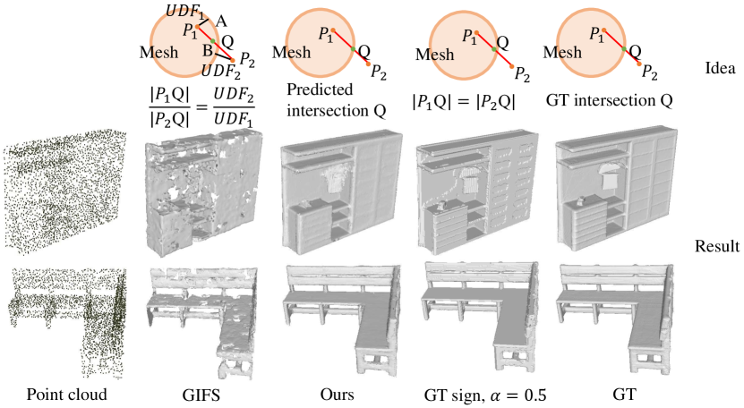
Figure 1: The idea and reconstruction quality of GIFS [28], $\alpha=0.5$, ours and ground-truth, where $\alpha=\frac{|P_{1}Q|}{|P_{1}P_{2}|}$. We can see that ours reconstructs surface with better details and less artifacts.

1 Introduction

Surface reconstruction from point clouds is a long-standing and essential task that has been studied for many years. It plays a crucial role in various modern applications, including visual navigation and robotics. Numerous notable works [13, 15, 14, 7, 17, 1, 2, 27, 23, 24, 20, 25] have significantly advanced this field. Among the traditional methods, Poisson Surface Reconstruction [11], a well-known approach, has yielded good results. However, its performance may deteriorate in the absence of normals and faces with open-surface challenges. With the emergence of deep learning, many researchers have sought to enhance reconstruction results by leveraging the robust representation and predictive capabilities of deep neural networks. These methods can generally be categorized into SDF-based and UDF-based approaches in terms of geometry representation. UDF-based methods excel at representing open surfaces, whereas SDF-based methods struggle in this regard. Yet, predicting UDF values near the surface often introduces noise, despite the critical role these values play in achieving high-quality surface reconstruction. In this study, a novel approach is proposed to enhance surface reconstruction by directly predicting the intersection points between surfaces and line segments. This method not only improves reconstruction quality but also maintains the capacity to represent open surfaces effectively.

Most methods for reconstructing surfaces from point clouds ultimately rely on Marching Cubes or its variants. Marching Cubes require two key pieces of information to generate a triangle mesh. As depicted in Fig. 2 (b), the first piece is the sign of the eight corners in a cube, while the second is the intersection points between the surface and the edges of the cube, such as the exact position of point P after determining that P lies on line AB in Fig. 2 (b). Therefore, in order to achieve better surface reconstruction, it is crucial to enhance the accuracy of both the sign of the eight corners in a cube and the exact intersection positions. While most researchers agree on the importance of the accuracy of the sign of the eight corners in a cube, the significance of the exact intersection position is often overlooked. However, the second aspect is equally important. This can be illustrated through a simple comparison. As demonstrated in Fig. 1, the shape in the fourth column is reconstructed using Marching Cubes with ground-truth signs, and all intersection points are precisely in the middle of the cube edges. On the other hand, the shape in the fifth column is reconstructed with ground-truth signs and ground-truth intersection positions. It is evident that the shape in the fifth column appears smoother, whereas the one in the fourth column exhibits numerous artifacts. These artifacts mainly stem from incorrect intersection positions when $\alpha=0.5$, where $\alpha=\frac{|P_{1}Q|}{|P_{1}P_{2}|}$ in Fig. 1. Therefore, the accuracy of intersection positions significantly impacts the quality of surface reconstruction.

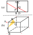
Figure 2: (a) aims to clarify the intersection module symmetry is necessary. (b) indicate the two parts, cube corner sign and intersection position, we need to predict in reconstructing mesh

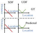
Figure 3: When predicting UDF near the zero-level set, it is easy to generate lots errors due to discontinuity of gradient near the zero-level set.

It is a common phenomenon that predicting the UDF in the vicinity of the surface tends to introduce noise. This is due to the discontinuity of the UDF gradient near the surface. When using a neural network to represent the UDF, accurately predicting the sharp changes near the zero-level set becomes challenging. This issue is illustrated in Fig. 3. The CAP method [31] also highlights this challenge. The presence of UDF noise near the surface can lead to incorrect intersection points between the cube edge and the surface, ultimately resulting in artifacts in the reconstructed mesh. This discrepancy explains why SDF-based methods typically yield smoother results compared to UDF-based approaches.

Although UDF can represent a wider range of surfaces than SDF, it tends to introduce noise near the surface due to the discontinuity of its gradient around the surface. Therefore, we have chosen to avoid predicting UDF and instead focus on directly predicting the intersection points between surfaces and cube edges. The pipeline is illustrated in Fig. 4. This approach allows us to maintain the ability to represent open surfaces while generating smoother surfaces with fewer artifacts compared to UDF-based methods. Furthermore, to ensure surface continuity, we have implemented a special design to predict intersections with a property similar to an odd function. In summary, we can list our main contribution here,

• Initially proposed to directly predict the intersection point between the cube edge and the surface, leading to enhanced accuracy in determining the intersection point.

• Developed a specialized module designed to predict these intersections while maintaining the surface’s continuity.

• Successfully achieved high-quality reconstruction results on three datasets: ShapeNet, MGN, and ScanNet.

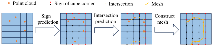
Figure 4: The pipeline of our method. First, we predict the relative sign of the cube. Then, we predict the intersection between the segment of point pair and implicit surface. Finally, we construct the mesh using the template in Marching Cube.

2 Related Works

Traditional point cloud reconstruction.

Point cloud reconstruction has been a persistent challenge in the fields of graphics and computer vision. Among the traditional methods, Poisson surface reconstruction [11] and ball-pivoting reconstruction [3] stand out as the most significant. The Poisson surface reconstruction method categorizes the query points based on the Poisson indicator function, while the ball-pivoting method generates a continuous surface by simulating a ball rolling over the points. Although these approaches yield satisfactory surface reconstructions, there is still room for further enhancement in performance.

SDF-based implicit surface reconstruction.

Implicit surface reconstruction methods based on signed distance functions (SDF) utilize deep learning techniques to either classify the occupancy of query points or directly predict the SDF value. These methods can be categorized into global approaches, which leverage overall shape information to classify query points, and local approaches, which classify query points based on their neighboring points.

Prominent global methods in this field include DeepSDF[21] and BSP-Net[6], which extract shape features and reconstruct the surface from these features. On the other hand, ConvOccNet[22], SSR-Net[20], DeepMLS[15], and POCO[4] are representative local methods. ConvOccNet[22] converts point cloud features into voxels and enhances features through volume convolution. SSR-Net[20] extracts point features, maps neighborhood point features to octants, and classifies them accordingly. DeepMLS[15] predicts normal and radius for each point and classifies query points based on the moving least-squares equation.

In addition to global and local methods, there are techniques that combine both global and local information, such as Points2Surf[9]. This method aims to regress the absolute SDF value using local information and determine the sign using global information.

Other SDF-based implicit surface reconstruction methods include SAL[1], SALD[2], and On-Surface Prior[18], which aim to transform explicit representations like point clouds and 3D triangle soups into implicit SDF representations. These methods require unique training processes and network parameters for each 3D model. SAL[1] employs MLP to predict shape SDFs with UDF-based metric supervision, while SALD[2] adds a derivative regularization term. On-Surface Prior[18] utilizes a pre-trained UDF-based network to improve SDF predictions.

While SDF methods have shown significant advancements in point cloud reconstruction, they have limitations in representing open surfaces or partial scans. This is important in realistic application, because we usually cannot guarantee that the scan is watertight.

UDF-based implicit surface reconstruction.

UDF has been a focal point in the realm of surface representation due to its ability to capture more general surfaces, including open surfaces and partial scans. Various research efforts have delved into leveraging UDF for implicit surface reconstruction. For instance, NDF [7] utilizes UDF to encode surface information and introduces a method for up-sampling point clouds during mesh reconstruction, employing the Ball Pivoting [3] technique. On the other hand, DUDE [27] adopts a volumetric UDF representation encoded within a neural network to describe shapes, leading to promising results in implicit surface reconstruction tasks. Nevertheless, a common challenge across these approaches is the reliance on 3D ground truth labels for training. Furthermore, a key unresolved issue pertains to the direct extraction of iso-surfaces from UDF. In a different approach, UWED [24] leverages Moving Least Squares (MLS) to convert UDF into a dense point cloud, showcasing an alternative strategy for handling UDF representations in surface reconstruction tasks.

3 Methods

3.1 Overview

In this section, we will initially present the complete pipeline of our method. Subsequently, we will delve into the prediction of intersection points and the pair-based sampling technique. Following that, we will discuss the two distinct components: predicting the sign and the intersection point individually. Lastly, we will elucidate the training loss.

3.2 Architecture

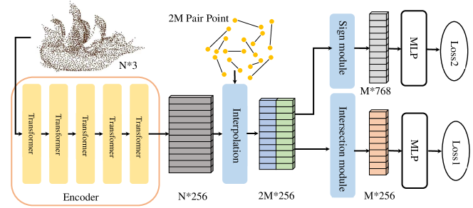
Figure 5: The UDF estimation network. Given the input point cloud $\mathcal{P}$ and the upsampled point cloud $\mathcal{P}_{\text{upsample}}$, the network estimates the per-point UDF projection flow in two stages with the guidance of the predicted approaching vector and the point-wise feature, respectively.

The network architecture is depicted in a straightforward manner, as illustrated in Fig. 5. Initially, the input point cloud with a total of $N$ points is inputted into the encoder to extract features with a dimension of $N*256$. The encoder comprises 4 transformer layers[30, 29], outputting dimensions of $64$, $256$, $256$, and $256$ respectively. Following a similar approach to GIFS [28], we adopt a paired query point sampling method, generating a total of $M$ pairs. Subsequently, an interpolation layer is employed to derive the features of the $2M$ query points. The network then diverges into two distinct paths. In the upper path, the focus is on predicting the relationship between the two points. The feature of the point pair is fed into the sign module to capture the relationship between the points. A multi-layer perceptron (MLP) is utilized to predict whether the two points exhibit the same sign, with a binary cross-entropy loss function applied. In the bottom path, the aim is to predict the position of the intersection point. The feature of the point pair is inputted into the intersection module, followed by the use of an MLP to predict the relative distance from the starting point to the intersection point. A simple regression loss is employed for this prediction. However, in cases where no intersection occurs between the cube edge and the surface, this term is disregarded in the loss calculation.

3.3 Pair Prediction

To sample point pairs for training and testing, we start by considering a point cloud $\mathcal{P}=\{p_{1},p_{2},\cdots,p_{N}\}$. During training, we uniformly sample points around $\mathcal{P}$ at varying scales and ratios. For each point $p_{i}$, a query point $q=p_{i}+U(-1,1)*s$ is randomly sampled, where $s$ takes values of 0.005, 0.01, and 0.02, corresponding to sample ratios of 0.6, 0.3, and 0.1 respectively. Subsequently, a cube with an edge length of 1/256 and $q$ as the upper-left corner is generated, allowing us to sample 12 point pairs corresponding to the 12 edges of the cube. Following this, we determine the intersection point of each edge with the surface and assess whether the point pairs lie on the same side of the surface.

During testing, to reconstruct the entire surface within the given space, we begin by identifying the bounding box of the shape and dividing it into cube meshes with an edge length of 1/256. For each cube within the bounding box, we predict the sign of the cube’s corners and the intersection positions. Utilizing the template matching method in Marching Cubes, we can then generate the triangle mesh. After sampling, we will elaborate on the specific predictions made by our network. Illustrated in Fig. 5, the lower pathway involves selecting a point pair AB, with point $A$ designated as the starting point and $B$ as the endpoint. The intersection point is denoted as $P$, and our aim is to forecast the proportionate distance from $A$ to $P$, expressed as $\frac{|AP|}{|AB|}$. Furthermore, as depicted in Fig. 5, within the upper pathway, we predict whether the point pairs lie on the same or different sides of the surface. The sign module’s name suggests that we solely predict the relationship between the corners of the cube and the upper-left corner within the cube. It is not the sign in the global view but a relative sign to the upper-left corner.

3.4 Sign Module

In the sign module, we formalize the problem as follows: given a start point $A$ and an end point $B$ with features $f_{A}$ and $f_{B}$ respectively, we denote the sign module as $G(f_{A},f_{B})$. The sign module $G(f_{A},f_{B})$ is required to exhibit the following property: when the positions of $A$ and $B$ are exchanged, $G(f_{A},f_{B})$ should vanish, i.e., $G(f_{A},f_{B})=G(f_{B},f_{A})$. This is because the relationship between $A$ and $B$ remains unchanged when their positions are swapped. To maintain this property and enhance the expressive capacity of $G(\cdot,\cdot)$, we design the sign module as follows:

$$G(f_{A},f_{B})=concat(f_{A}+f_{B}+pos,f_{A}*f_{B}+pos,max(f_{A},f_{B})+pos),$$ (1)

where $pos$ is the positional encoding[26] of $A-B$. Here, in order to keep the property $G(f_{A},f_{B})=G(f_{B},f_{A})$, we abandon the traditional sin-cos positional encoding and adopt only cosine positional encoding. Specifically, $pos(A,B)=cos(\frac{A-B}{2^{i}})$, $i\in\{1,2,\cdots,19\}$.

3.5 Intersection Module

In the intersection module, we aim to predict the position of the intersection point $P$ between point pair $A$ and $B$, each associated with features $f_{A}$ and $f_{B}$ respectively. The position of $P$ is represented by $\alpha\in[0,1]$, where $\alpha=\frac{|PA|}{|AB|}$. To ensure the continuity of the surface, we define the intersection module as $H(f_{A},f_{B})$, which should satisfy the property $H(f_{A},f_{B})=1-H(f_{B},f_{A})$. This condition is crucial for maintaining surface continuity. The relationship can be intuitively understood by observing that $\frac{|PA|}{|AB|}=1-\frac{|PB|}{|AB|}$. Based on this, we formulate the design of the intersection module as follows,

$$H(f_{A},f_{B})=sigmoid(f_{A}-f_{B}+pos_{2}),$$ (2)

where $pos_{2}$ is also the positional encoding of $A-B$. However, in this part, in order to keep the property $H(f_{A},f_{B})=1-H(f_{B},f_{A})$, we adopt only sine positional encoding. Specifically, $pos_{2}(A,B)=sin(\frac{A-B}{2^{i}})$, $i\in\{0,2,\cdots,19\}$.

Next, we can delve into the explanation for why a surface may not exhibit continuity if $H(f_{A},f_{B})\neq 1-H(f_{B},f_{A})$. Referring to Fig. 2 (a), the black cubes represent adjacent cubes in the Marching Cube algorithm. It is evident that $A$ is equivalent to $C$ and $B$ is equivalent to $D$. If a mesh is depicted by the red line, points $P$ and $Q$ must coincide; otherwise, the mesh will lack continuity. Therefore, the relationship $\frac{|AP|}{|AB|}=1-\frac{|DQ|}{|CD|}$ must be upheld. This condition serves as both necessary and sufficient for ensuring $H(f_{A},f_{B})=1-H(f_{B},f_{A})$.

3.6 Losses

In this approach, we utilize two types of loss functions for training. For sign prediction, we employ a straightforward binary cross-entropy loss. For intersection prediction, we apply a regression loss to minimize the disparity between the predicted $\alpha_{j}$ and the ground-truth $\alpha_{j_{GT}}$, as illustrated below:

$$Loss_{1}=\sum_{j=1}^{M}[\alpha_{j}-\alpha_{j_{GT}}]_{+},$$ (3)

where $\alpha_{j}$ means the predicted intersection position of $j-th$ point pair, $\alpha_{j_{GT}}$ means the ground-truth intersection position of $j-th$ point pair,

$$[\alpha-\alpha_{GT}]_{+}=\left\{\begin{array}[]{lc}|\alpha-\alpha_{GT}|&\alpha_{GT}\in[0,1]\\ 0&\alpha_{GT}\notin[0,1].\\ \end{array}\right.$$ (4)

4 Experiments

4.1 Dataset and Experiment Settings

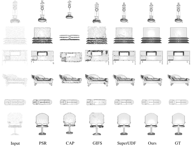
Figure 6: Visualized results of our method and state-of-the-art alternatives. Note that we provide the ground-truth normal as input for PSR as it requires. Methods are PSR[11], CAP[31], GIFS[28], SuperUDF[10]. The number of input point cloud is 3000.

Our methodology is assessed on three prominent open-source datasets. Initially, we randomly select 1300 shapes from 13 distinct categories within the ShapeNet dataset [5], with each category comprising 100 shapes. The point number of each input point cloud is 3000. Subsequently, we employ the MGN dataset, encompassing both pants and shirts. The point number of each input point cloud is 3000. Finally, we include 100 scenes from the real-world ScanNet dataset [8], obtained through scanning technology, resulting in 10,000 input point clouds. To facilitate a comprehensive comparison with existing techniques, we utilize standard evaluation metrics commonly employed in surface reconstruction. One such metric is Chamfer-$L_{1}$ ($CD_{1}$), which measures the distance between two sets of points. Additionally, to demonstrate enhancements in artifact elimination, we utilize normal consistency ($NC$) as a metric to evaluate the smoothness of the reconstructed surface.

When calculating $CD_{1}$, we follow O-Net[19] and randomly sample 100000 points on the reconstructed mesh and 100000 points on ground-truth mesh. $CD_{1}$ equation is shown as the Eq.5

$$\mathrm{CD}_{1}= \frac{1}{2N_{x}}\sum_{i=1}^{N_{x}}\left\|\mathbf{x}_{i}-\mathcal{S}_{y}\left(\mathbf{x}_{i}\right)\right\|_{1}+$$ (5)

$$\frac{1}{2N_{y}}\sum_{i=1}^{N_{y}}\left\|\mathbf{y}_{i}-\mathcal{S}_{x}\left(\mathbf{y}_{i}\right)\right\|_{1},$$

$\{\mathbf{x}_{i},i=0\cdots N_{x}\}$ is the points set sampled from ground-truth mesh. $\{\mathbf{y}_{i},i=0\cdots N_{y}\}$ is the point set sampled from reconstructed mesh. $\mathcal{S}_{y}(\mathbf{x}_{i})$ means the nearest point to $\mathbf{x}_{i}$ in reconstructed point set. $\mathcal{S}_{x}(\mathbf{y}_{i})$ means the nearest point to $\mathbf{y}_{i}$ in ground-truth point set. $\|\cdot\|_{1}$ means $L1-distance$.

Normal consistency is closely related to $CD_{1}$, shown in Eq.6

$$\mathrm{NC}= \frac{1}{2N_{x}}\sum_{i=1}^{N_{x}}|<\mathbf{n}\left(\mathbf{x}_{i}),\mathbf{n}(\mathcal{S}_{y}\left(\mathbf{x}_{i}\right)\right)>|+$$ (6)

$$\frac{1}{2N_{y}}\sum_{i=1}^{N_{y}}|<\mathbf{n}\left(\mathbf{y}_{i}),\mathbf{n}(\mathcal{S}_{x}\left(\mathbf{y}_{i}\right)\right)>|.$$

$\mathbf{n}(x)$ means the normal of point $x$. $<,>$ means inner-product. Here, we calculate the absolute value of inner product, because our mesh is not orientated.

4.2 Watertight Surface Reconstruction

Indicator	$CD_{1}\downarrow$					$NC\uparrow$
Class	GIFS	CAP	PSR	SuperUDF	Ours	GIFS	CAP	PSR	SuperUDF	Ours
	[28]	[31]	[11]	[10]		[28]	[31]	[11]	[10]
airplane	0.0026	0.0031	0.0023	0.0022	0.0012	0.9322	0.9318	0.9435	0.9469	0.9716
bench	0.0058	0.0059	0.0037	0.0029	0.0019	0.8865	0.8874	0.9062	0.9234	0.9449
cabinet	0.0104	0.0048	0.0056	0.0039	0.0026	0.9370	0.9331	0.9357	0.9456	0.9700
car	0.0052	0.0054	0.0039	0.0029	0.0024	0.8825	0.8879	0.8975	0.9014	0.9133
chair	0.0041	0.0042	0.0053	0.0039	0.0024	0.9415	0.9447	0.9311	0.9498	0.9601
display	0.0055	0.0047	0.0043	0.0034	0.0021	0.9456	0.9513	0.9643	0.9712	0.9834
lamp	0.0078	0.0082	0.0036	0.0030	0.0018	0.9108	0.9025	0.9366	0.9334	0.9476
speaker	0.0081	0.0063	0.0050	0.0041	0.0026	0.9015	0.9243	0.9531	0.9589	0.9712
rifle	0.0029	0.0013	0.0012	0.0011	0.0009	0.9345	0.9533	0.9685	0.9668	0.9776
sofa	0.0069	0.0050	0.0038	0.0033	0.0022	0.9370	0.9413	0.9534	0.9520	0.9758
table	0.0065	0.0088	0.0043	0.0025	0.0023	0.9235	0.9109	0.9381	0.9428	0.9749
phone	0.0049	0.0024	0.0024	0.0021	0.0017	0.9537	0.9725	0.9790	0.9713	0.9869
vessel	0.0033	0.0025	0.0012	0.0021	0.0015	0.9167	0.9355	0.9464	0.9487	0.9625
Mean	0.0057	0.0048	0.0037	0.0028	0.0019	0.9239	0.9284	0.9423	0.9470	0.9648

Table 1: $CD_{1}$ and $NC$ comparison on ShapeNet within 13 classes. $\downarrow$ means lower is better. $\uparrow$ means higher is better.

Several previous studies [21, 22, 19, 7] have commonly utilized the watertight surface reconstruction approach for implicit surface reconstruction, a key focus of this point cloud reconstruction research. In order to evaluate the effectiveness of our proposed method, we conducted a comprehensive analysis of watertight surface reconstruction using the ShapeNet dataset [5]. Specifically, we uniformly sampled 3000 points from the watertight mesh to serve as input data. We compared our method against four well-known techniques, excluding PSR [11], all of which are UDF-based methods. The methods included GIFS [28], CAP [31], and SuperUDF [10]. For the PSR [11] method, we incorporated ground-truth normals as input data. The visualization results are presented in Fig. 6. Our method not only preserves more details but also produces smoother results. The quantitative evaluation results are summarized in Table 1. These results demonstrate that our method achieves excellent performance across all 13 classes with a significant margin, showcasing its state-of-the-art capabilities. Particularly noteworthy is the performance on the $NC$, indicating that our reconstructed surfaces are not only faithful to the ground truth but also exhibit smoothness.

4.3 Open Surface Reconstruction

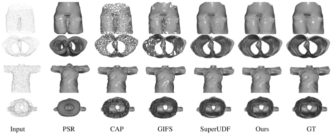
Figure 7: Visualized results of our method and state-of-the-art alternatives. Note that we provide the ground-truth normal as input for PSR as it requires. Methods are PSR[11], CAP[31], GIFS[28], SuperUDF[10]. The number of input point cloud is 3000.

	CAP [31]	PSR [11]	GIFS [28]	SUDF[10]	Ours
$CD_{1}\downarrow$	0.0035	0.0045	0.0033	0.0024	0.0019
$NC\uparrow$	0.9407	0.9356	0.9418	0.9645	0.9758

Table 2: $CD_{1}$ and $NC$ comparison results on MGN dataset.

By leveraging a pair-point structure akin to GIFS for representing surfaces within our framework, we are able to proficiently reconstruct open surfaces. We achieve this by uniformly sampling 3000 points on each MGN mesh to reconstruct the implicit surface, a task that poses challenges for SDF-based methods given the characteristics of open surfaces. The comparative analysis presented in Table 2 illustrates the superior performance of our approach in comparison to various methods including PSR [11], CAP [31], GIFS [28], and SuperUDF [10]. Moreover, the visual results depicted in Fig.  7 exhibit the faithfulness of our reconstructed mesh, capturing intricate details and closely mirroring the ground-truth.

4.4 Scene Reconstruction

Real scene reconstruction is characterized by a heightened level of complexity, primarily due to the inherent openness and incompleteness of the input point cloud data. In this study, we meticulously selected 100 scenes from ScanNet and illustrated the visualization results in Fig. 8, along with the quantitative results in Table 3, in comparison with other methods.

Upon examining the visualization results, our reconstructed surface exhibits a notably smoother appearance compared to other methods. Furthermore, the quantitative analysis reveals that our approach outperforms other methods in terms of both $CD_{1}$ and $NC$, underscoring the efficacy of our design in accurately predicting the intersection points between the surface and cube edges.

	CAP [31]	PSR [11]	GIFS [28]	SuperUDF [10]	Ours
$CD_{1}\downarrow$	0.0044	0.0240	0.0043	0.0039	0.0037
$NC\uparrow$	0.8679	0.8420	0.8713	0.8722	0.8810

Table 3: $CD_{1}$ comparison on ScanNet with different number of sample point.

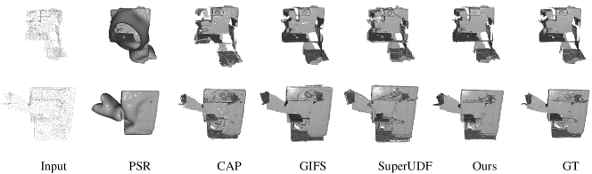
Figure 8: Visualized results of our method and state-of-the-art alternatives. Note that we provide the ground-truth normal as input for PSR as it requires. Methods are PSR[11], CAP[31], GIFS[28], SuperUDF[10]. The number of input point cloud is 3000.

4.5 Ablation Study

Contribution of sign module and intersection module.

To enhance the quality of surface reconstruction, it is essential to predict the sign of cube corners. This allows for the selection of appropriate triangle templates akin to the Marching Cube algorithm. Additionally, accurate intersection point prediction is crucial. By leveraging this information, adjustments can be made to the triangle positions, resulting in smoother surfaces with reduced artifacts. Our approach consists of two key components: the sign module and the intersection module. Consequently, we aim to conduct experiments to evaluate the impact of each component on surface quality. In pursuit of this objective, we have devised 9 comparative experiments to demonstrate the contributions of each component, as presented in Table 4 and Table 5. Upon examining the results row-wise, it is evident that regardless of the chosen sign prediction method, our intersection results outperform those of GIFS [28]. Furthermore, the disparity between our intersection prediction outcomes and ground truth (GT) predictions is minimal, indicating the enhanced accuracy of our intersection module. When analyzing the results column-wise, it is apparent that regardless of the chosen intersection prediction method, our sign prediction results surpass those of GIFS [28]. Moreover, the difference between our sign prediction outcomes and GT sign predictions is negligible, highlighting the efficacy of our sign module in improving sign prediction accuracy.

$CD_{1}\downarrow$	GIFS Intersection	Our Intersection	GT Intersection
GIFS Sign	0.0057	0.0042	0.0037
Our Sign	0.0025	0.0019	0.0018
GT Sign	0.0023	0.0018	0.0017

Table 4: The contribution of sign module and intersection module. The $CD_{1}$ is obtained on ShapeNet 13 classes.

$NC\uparrow$	GIFS Intersection	Our Intersection	GT Intersection
GIFS Sign	0.9239	0.9312	0.9403
Our Sign	0.9435	0.9648	0.9703
GT Sign	0.9677	0.9801	0.9812

Table 5: The contribution of sign module and intersection module. The $NC$ is obtained on ShapeNet 13 classes.

Accuracy of intersection point.

Except for the final metrics $CD_{1}$ and $NC$ on the mesh, we also present intermediate results to demonstrate the enhancements made to the intersection module. When reconstructing the mesh, both UDF-based methods and ours attempt to compute the intersection point of the surface and the cube edge. The key difference lies in the approach: the UDF-based method determines the intersection position by inversely considering the UDF value between two points, while our method directly predicts the intersection using a neural network. Specifically, we evaluate the distance between the predicted intersection point and the ground-truth intersection point generated by different methods in Table 6. To elaborate, we initially divide the space into cubes with a resolution of 256. Subsequently, for each cube edge intersecting with the implicit surface, we calculate the distance from the predicted intersection to the ground-truth intersection as $d=|p_{\text{predicted}}-p_{\text{gt}}|\times 256$. These results are obtained from the ShapeNet dataset. It is evident that our method significantly enhances the accuracy of the intersection point.

Method	GIFS [28]	SuperUDF[10]	CAP [31]	Ours
Distance $\downarrow$	0.0131	0.0127	0.0095	0.0084

Table 6: The distance from predicted intersection to GT intersection on ShapeNet.

Method	$CD_{1}\downarrow$	$NC\uparrow$
$\hat{G}(f_{A},f_{B})$	0.0023	0.9573
$G(f_{A},f_{B})$	0.0019	0.9648

Table 7: The reconstruction result comparison when sign module is invariant or variant to the exchange of start and end point. The result is average on 13 classes of ShapeNet.

Method	$CD_{1}\downarrow$	$NC\uparrow$
$\hat{H}(f_{A},f_{B})$	0.0024	0.9425
$H(f_{A},f_{B})$	0.0019	0.9648

Table 8: The Comparison when intersection module satisfies $H(f_{A},f_{B})=1-H(f_{B},f_{A})$ or not. The result is average on 13 classes of ShapeNet.

Sign module in-variance.

In our design, the sign module remains invariant when the start point and end point exchange their positions, i.e., $G(f_{A},f_{B})=G(f_{B},f_{A})$. Here, we aim to quantitatively evaluate the influence of this design feature. Therefore, we compare the reconstruction results when $G(\cdot,\cdot)$ does not maintain this invariance with the results when $G(\cdot,\cdot)$ does maintain this invariance. Specifically, when $G(\cdot,\cdot)$ does not maintain the invariance, we set

$$\hat{G}(f_{A},f_{B})=concat(f_{A}+pos_{3},f_{B}+pos_{3}),$$ (7)

where $pos_{3}$ is the standard positional encoding of both sine and cosine encoding. The quantitative result is in Table 7. We can see the invariance works.

Intersection module symmetry.

In our design, the intersection module exhibits the symmetry of the point pair, i.e., $H(f_{A},f_{B})=1-H(f_{B},f_{A})$. This symmetry is ensured by the Sigmoid activation function and the unique design of positional encoding. Here, we seek to assess the influence of this symmetry. Therefore, we compare the results when the symmetry is absent versus when it is present. Specifically, we define the function $\hat{H}(\cdot,\cdot)$ as

$$\hat{H}(f_{A},f_{B})=sigmoid(concat(f_{A}+pos_{3},f_{B}+pos_{3})).$$ (8)

The quantitative result is in Table 8 and visualization result is in Fig. 9, we can see that the discontinuity indeed appear when the symmetry is absent.

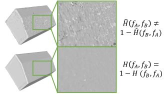
Figure 9: When the intersection module satisfy $H(f_{A},f_{B})=1-H(f_{B},f_{A})$, the surface is continuous, otherwise it is not continuous and has lots of errors.

5 Conclusion and Limitations

This study introduces a method that predicts the intersection between a segment of a point pair and an implicit surface to effectively eliminate artifacts. Additionally, it proposes two novel modules that utilize neural networks to predict the sign of cube corners and intersections. This approach results in a more detailed surface reconstruction with fewer artifacts, leading to excellent outcomes on three datasets: ShapeNet, MGN, and ScanNet. However, there are some limitations to this method. It performs accurately when the surface is parallel to the bounding box face; yet, significant changes in the angle between the tangent plane of the surface and the bounding box face in a local region can lead to errors in intersection prediction, resulting in a less smooth surface. This issue will be addressed in future research. Furthermore, the method struggles to generate satisfactory meshes near the edges of open surfaces.

Appendix 0.A Details

Training.

During training, we utilize 16,000 randomly sampled point pairs every iteration. The trainig epoch is 100. We employ the Adam optimizer [12] and incorporate cosine learning rate adjustment [16]. The initial learning rate is set to 0.001, and the batch size is 1.

Testing.

During testing, to assess the quality of the reconstructed mesh, we randomly sample 100,000 points with normals on both the reconstructed mesh and the ground-truth mesh. Subsequently, we calculate the Chamfer Distance ($CD_{1}$) and Normal Consistency ($NC$) between these point sets.

Training/Testing splitting.

During training, we sampled 1300 shapes for ShapeNet, 71 for MGN, and 100 for ScanNet, respectively. For testing, the same number of shapes was sampled. It is important to note that the shapes used for training and testing do not overlap.

Two prediction ways.

In fact, we have experimented with two methods for constructing the mesh. The first method involves first predicting the relative sign of the cube corners and then predicting the intersection point when the point pair is on different sides of the surface, with the intersection parameter $\alpha\in[0,1]$. On the other hand, the second method directly predicts the intersection parameter $\alpha\in\mathbb{R}$ without the need to predict the cube corner sign first. By observing that if $\alpha\in[0,1]$, an intersection exists between the two points, while no intersection point exists for other values of $\alpha$, we found that the convergence of the second method was unsatisfactory in our experiments. Therefore, we have decided to adopt the first method for constructing the mesh.

Similarities and differences between GIFS [28].

Our approach shares a common point with GIFS in that both methods involve predicting the relative sign of a point pair, indicating whether the two points are on the same side or opposite sides of the surface. However, a key distinction between our method and GIFS lies in the approach to determining the intersection point: we directly predict the intersection between a segment and a surface, whereas GIFS utilizes $\alpha=\frac{UDF_{1}}{UDF_{2}}=\frac{|PA|}{|AB|}$ to define point $P$. Additionally, a minor difference is observed in the network architecture, as we employ a point transformer and interpolation layer to extract query point features, while GIFS utilizes 3D convolution for the same purpose.

Post-processing.

After generating the mesh, we design a method to remove the triangle soup which is obviously wrong. The idea is very simple. In short, if the normal of the triangle is far from its neighbors, we will remove this triangle. Specifically, we calculate the following indicator

$$I=\frac{1}{k}\sum_{i=0}^{k-1}|<n,n_{i}>|,$$ (9)

where $k$ is number of k-nearest neighbor, $<\cdot,\cdot>$ is inner-product. $n$ is the normal of triangle, $n_{i}$ is the normal of its neighbor triangles. If $I<0.65$, we will remove the triangle.

Appendix 0.B Additional visualization result

In order to show the quality of reconstructed mesh, we provide additional visualization result in Fig. 10, Fig. 11 and Fig. 12.

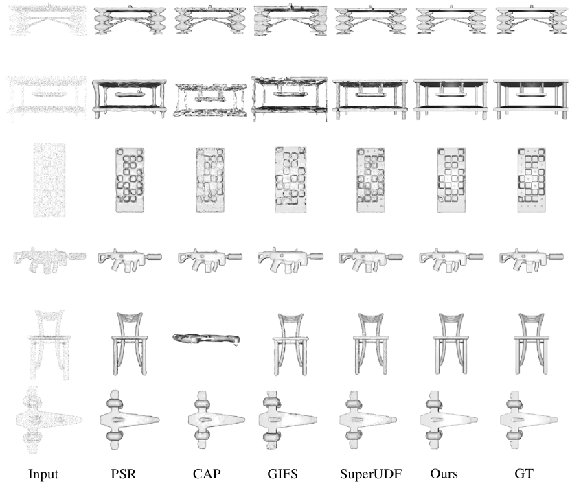
Figure 10: Visualized results of our method and state-of-the-art alternatives. Note that we provide the ground-truth normal as input for PSR as it requires. Methods are PSR[11], CAP[31], GIFS[28], SuperUDF[10]. The number of input point cloud is 3000.

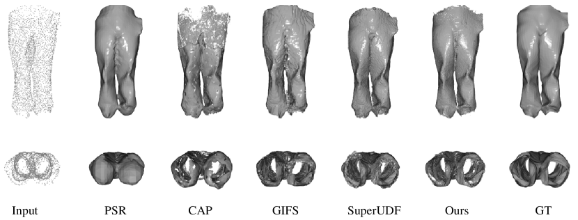
Figure 11: Visualized results of our method and state-of-the-art alternatives. Note that we provide the ground-truth normal as input for PSR as it requires. Methods are PSR[11], CAP[31], GIFS[28], SuperUDF[10]. The number of input point cloud is 3000.

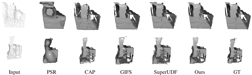
Figure 12: Visualized results of our method and state-of-the-art alternatives. Note that we provide the ground-truth normal as input for PSR as it requires. Methods are PSR[11], CAP[31], GIFS[28], SuperUDF[10]. The number of input point cloud is 10000.

Appendix 0.C Efficiency Analysis

Here, we present the GPU memory usage and time required for mesh reconstruction in Table 9. The average reconstruction time was calculated across 1300 shapes from ShapeNet. The experiments were conducted using a Titan X 12GB GPU and an Intel(R) i9-9900k@3.60GHz CPU. It is evident that our approach achieves high reconstruction speed, albeit at the expense of increased GPU memory utilization.

Method	GPU Memory(MB)	Inference Time(s)
GIFS [28]	3478	8min46s
CAP [31]	1398	21min56s
Ours	6756	6min52s

Table 9: The time and memory comparison between GIFS [28], CAP [31] and ours in inference. The result is on the ShapeNet.

References

- [1] Atzmon, M., Lipman, Y.: SAL: Sign Agnostic Learning of Shapes From Raw Data. In: 2020 IEEE/CVF Conference on Computer Vision and Pattern Recognition (CVPR). pp. 2562–2571. IEEE, Seattle, WA, USA (Jun 2020). https://doi.org/10.1109/CVPR42600.2020.00264
- [2] Atzmon, M., Lipman, Y.: SALD: Sign Agnostic Learning with Derivatives (Oct 2020)
- [3] Bernardini, F., Mittleman, J., Rushmeier, H., Silva, C., Taubin, G.: The ball-pivoting algorithm for surface reconstruction. Visualization and Computer Graphics, IEEE Transactions on (1999)
- [4] Boulch, A., Marlet, R.: Poco: Point convolution for surface reconstruction. In: Proceedings of the IEEE/CVF Conference on Computer Vision and Pattern Recognition (2022)
- [5] Chang, A.X., Funkhouser, T., Guibas, L., Hanrahan, P., Huang, Q., Li, Z., Savarese, S., Savva, M., Song, S., Su, H., et al.: Shapenet: An information-rich 3d model repository. arXiv preprint arXiv:1512.03012 (2015)
- [6] Chen, Z., Tagliasacchi, A., Zhang, H.: Bsp-net: Generating compact meshes via binary space partitioning. In: Proceedings of the IEEE/CVF Conference on Computer Vision and Pattern Recognition. pp. 45–54 (2020)
- [7] Chibane, J., Mir, A., Pons-Moll, G.: Neural unsigned distance fields for implicit function learning (2020)
- [8] Dai, A., Chang, A.X., Savva, M., Halber, M., Funkhouser, T., Nießner, M.: Scannet: Richly-annotated 3d reconstructions of indoor scenes. In: Proc. Computer Vision and Pattern Recognition (CVPR), IEEE (2017)
- [9] Erler, P., Guerrero, P., Ohrhallinger, S., Wimmer, M., Mitra, N.J.: Points2surf: Learning implicit surfaces from point cloud patches (2020)
- [10] Hui Tian, Chenyang Zhui, Y.S., Xu, K.: Superudf: Self-supervised udf estimation for surface reconstruction. https://arxiv.org/abs/2308.14371 (2023)
- [11] Kazhdan, M., Bolitho, M., Hoppe, H.: Poisson surface reconstruction. The Japan Institute of Energy 67(224), 1517–1531 (2013)
- [12] Kingma, D.P., Ba, J.: Adam: A method for stochastic optimization. arXiv preprint arXiv:1412.6980 (2014)
- [13] Li, T., Wen, X., Liu, Y.S., Su, H., Han, Z.: Learning deep implicit functions for 3d shapes with dynamic code clouds. In: Proceedings of the IEEE/CVF Conference on Computer Vision and Pattern Recognition (2022)
- [14] Liao, Y., Donné, S., Geiger, A.: Deep marching cubes: Learning explicit surface representations. In: 2018 IEEE/CVF Conference on Computer Vision and Pattern Recognition (2018)
- [15] Liu, S.L., Guo, H.X., Pan, H., Wang, P.S., Tong, X., Liu, Y.: Deep implicit moving least-squares functions for 3d reconstruction. In: Proceedings of the IEEE/CVF Conference on Computer Vision and Pattern Recognition. pp. 1788–1797 (2021)
- [16] Loshchilov, I., Hutter, F.: Sgdr: Stochastic gradient descent with restarts (2016)
- [17] Ma, B., Han, Z., Liu, Y.S., Zwicker, M.: Neural-pull: Learning signed distance functions from point clouds by learning to pull space onto surfaces (2020)
- [18] Ma, B., Liu, Y.S., Han, Z.: Reconstructing Surfaces for Sparse Point Clouds With On-Surface Priors. In: 2022 IEEE/CVF Conference on Computer Vision and Pattern Recognition. p. 11
- [19] Mescheder, L., Oechsle, M., Niemeyer, M., Nowozin, S., Geiger, A.: Occupancy networks: Learning 3d reconstruction in function space. In: 2019 IEEE/CVF Conference on Computer Vision and Pattern Recognition (CVPR) (2019)
- [20] Mi, Z., Luo, Y., Tao, W.: Ssrnet: Scalable 3d surface reconstruction network. In: 2020 IEEE/CVF Conference on Computer Vision and Pattern Recognition (CVPR) (2020)
- [21] Park, J., Florence, P., Straub, J., Newcombe, R., Lovegrove, S.: Deepsdf: Learning continuous signed distance functions for shape representation. In: 2019 IEEE/CVF Conference on Computer Vision and Pattern Recognition (CVPR) (2019)
- [22] Peng, S., Niemeyer, M., Mescheder, L., Pollefeys, M., Geiger, A.: Convolutional Occupancy Networks (2020)
- [23] Peng-Shuai Wang, Yang Liu, X.T.: Dual octree graph networks for learning adaptive volumetric shape representations. In: ACM Transactions on Graphics (2022)
- [24] Richa, J.P., Deschaud, J.E., Goulette, F., Dalmasso, N.: UWED: Unsigned Distance Field for Accurate 3D Scene Representation and Completion p. 20
- [25] T Zhao, L Busé, D.C.S.T.B.J.T.P.A.: Variational shape reconstruction via quadric error. In: ACM SIGGRAPH 2023 Conference Proceedings. pp. 1–10 (2023)
- [26] Tancik, M., Srinivasan, P.P., Mildenhall, B., Fridovich-Keil, S., Raghavan, N., Singhal, U., Ramamoorthi, R., Barron, J.T., Ng, R.: Fourier features let networks learn high frequency functions in low dimensional domains (2020)
- [27] Venkatesh, R., Sharma, S., Ghosh, A., Jeni, L., Singh, M.: DUDE: Deep Unsigned Distance Embeddings for Hi-Fidelity Representation of Complex 3D Surfaces (Dec 2020)
- [28] Ye, J., Chen, Y., Wang, N., Wang, X.: GIFS: Neural Implicit Function for General Shape Representation. In: Proceedings of the IEEE/CVF Conference on Computer Vision and Pattern Recognition. p. 11 (2022)
- [29] Zhao, H., Jia, J., Koltun, V.: Exploring self-attention for image recognition (2020)
- [30] Zhao, H., Jiang, L., Jia, J., Torr, P.H., Koltun, V.: Point transformer. In: Proceedings of the IEEE/CVF International Conference on Computer Vision. pp. 16259–16268 (2021)
- [31] Zhou, J., Ma, B., Yu-Shen, L., Yi, F., Zhizhong, H.: Learning consistency-aware unsigned distance functions progressively from raw point clouds. In: Advances in Neural Information Processing Systems (NeurIPS) (2022)