Hopfions of massive gauge bosons in early universe

Abstract

This letter presents a novel model that characterizes the curvature of space-time, influenced by a massive gauge field in the early universe. This curvature can lead to a multitude of observations, including the Hubble tension issue and the isotropic stochastic gravitational-wave background. We introduce, for the first time, the concept of gauge field Hopfions, which exist in the space-time. We further investigate how hopfions can influence Hubble parameter values. Our findings open the door to utilizing hopfions as a topological source which links both gravitation and the gauge field.

Introduction. During the inflationary period, the interplay between coupled axion and SU(2) gauge fields [1, 2] offers a diverse range of phenomena, distinguishing itself from the characteristics observed in conventional single scalar field inflation models [3, 4]. Notably, this coupling gives rise to intriguing outcomes, such as the generation of a stochastic background comprising chiral gravitational waves [5, 6], characterized by their non-Gaussian nature [7, 8]. Moreover, recent studies [9, 10, 11] have demonstrated that the production of these chiral gravitational waves results in a non-zero parity-violating gravitational anomaly. This anomaly breaks lepton number symmetry and helps to explain the observed baryon asymmetry in the universe. Massless gauge bosons generate gravitational wave signals, as studied in [12, 13]. Gravitational waves from tensor perturbations are a common outcome of simple inflation models. In [14], they show how massive gauge bosons also produce gravitational wave signals through tensor fluctuations during inflation. Massive particles are usually hard to produce during inflation due to a Boltzmann-like factor $exp(-\pi m/H)$, where $m$ is the particle’s mass and $H$ is the Hubble rate, the inflationary scale. This reduces the signals at the cosmological collider. Within the realm of topological solitons, magnetic skyrmions are two-dimensional entities resembling particles, characterized by a continuous twist of magnetization. On the other hand, magnetic Hopfions are three-dimensional structures that can be constructed from a closed loop of intertwined skyrmion strings. Theoretical frameworks propose that magnetic Hopfions can achieve stability in frustrated or chiral magnetic systems, and that target skymions can be converted into Hopfions by adjusting their perpendicular magnetic anisotropy. However, experimental confirmation of these theories remains elusive to date [15, 16, 17].
Recently, there has been a significant orientation towards the study of magnetic Hopfions [18, 19, 20, 21, 22]. Our aim in this letter is to present, for the first time, the concept of gauge field Hopfions. These exist in space-time in the early universe and could potentially resolve the tension issue of Hubble and the signal from pulsar timing arrays.

Inflation with massive gauge bosons. We study how to generate a force field with mass using the Chern-Simons interaction. We use a U(1) gauge field $A_{\mu}$ and add a term $\phi F_{\mu\nu}\tilde{F}^{\mu\nu}$ that connects it with the inflaton field $\phi$ [23, 14]

$$S = \int d^{4}x\sqrt{-g}(-\frac{1}{2}\partial_{\mu}\phi\partial^{\mu}\phi-V\left(\phi\right)-\frac{1}{4}F_{\mu\nu}F^{\mu\nu}.$$

$$-\frac{\sigma}{4\Lambda}\phi F_{\mu\nu}\tilde{F}^{\mu\nu}+\frac{1}{2}m_{A}^{2}A^{\mu}A_{\mu}).$$

Here, $\Lambda$ represents the mass scale that suppresses higher-dimensional operators in the theory, while $\sigma$ is the dimensionless coupling of the inflaton-gauge field. Here $A_{\mu}$ is U(1) gauge field $A_{\mu}$ and its field strength tensor $F_{\mu\nu}=\partial_{\mu}A_{\nu}-\partial_{\nu}A_{\mu}$. We also have its dual $\tilde{F}^{\mu\nu}=\frac{1}{2}\frac{\epsilon^{\mu\nu\alpha\beta}}{\sqrt{-g}}F_{\alpha\beta}$. We focus on the key role of $\frac{1}{2}m_{A}^{2}A^{\mu}A_{\mu}$, which connects the gauge field and the gravitational waves through the mass $m_{A}$. The energy of the Chern-Simons interaction is $-\frac{\sigma}{8\Lambda}\int d^{3}xe^{-i\mathbf{k\cdot x}}\delta\phi\epsilon^{\mu\nu\alpha\beta}F_{\mu\nu}F_{\alpha\beta}$. We consider a homogeneous and isotropic universe described by the Friedmann-Lemaître-Robertson-Walker (FLRW) metric $ds^{2}=-dt^{2}+a^{2}(t)g_{ij}dx^{i}dx^{j}$ where $a(t)$ is the scale factor and $H=da/dt$ is the Hubble parameter. We also assume the inflaton $\phi$ that only depends on time $t$. This field is similar to an axion, a light pseudoscalar particle with a shift symmetry $\phi\rightarrow\phi+\phi_{0}$. We take a simple quadratic potential for the inflaton, $V\left(\phi\right)=\frac{1}{2}m^{2}\phi^{2}$, where $m=1.9\times 10^{13}GeV\left(\propto\Lambda^{2}\right)$ [24]. The background dynamics of $\phi\left(t\right)$ and $A(t,x)$ [25] are given by

$$\ddot{\phi}+3H\dot{\phi}+\frac{dV\left(\phi\right)}{d\phi}-\frac{\nabla^{2}\phi}{a^{2}\left(t\right)}=\frac{\sigma}{\Lambda}\left\langle\mathbf{E\cdot B}\right\rangle,$$ (2)

$$3M_{p}^{2}H^{2}-\frac{1}{2}\dot{\phi}^{2}-V\left(\phi\right)-\frac{\left(\nabla\phi\right)^{2}}{2a^{2}\left(t\right)}=\frac{1}{2}\left\langle\mathbf{E}^{2}+\mathbf{B}^{2}+\frac{m_{A}^{2}}{a^{2}}\mathbf{A}^{2}\right\rangle,$$ (3)

where $\mathbf{E}=-\frac{\mathbf{A}\prime}{a^{2}}=-\frac{1}{a^{2}}\frac{\partial\mathbf{A}}{\partial\tau}$ and $\mathbf{B}=\frac{\mathbf{\nabla}\times\mathbf{A}}{a^{2}}$ are the electric and magnetic fields corresponding to the gauge field respectively. Here $M_{p}^{2}\approx 2.4\times 10^{18}GeV$ is the reduced Planck mass. We now consider that the evolution of the scale factor is written as a power law $a=a_{0}t^{q}$. That implies the Hubble parameter can rewrite as $H=\frac{1}{a\tau}$, where $\tau$ is the conformal time with $dt=a\left(\tau\right)d\tau$. The inflaton perturbations follow the equation of motion

$$\delta\ddot{\phi}+3\beta H\delta\dot{\phi}-\left(\frac{\nabla^{2}}{a^{2}}-\frac{d^{2}V\left(\phi\right)}{d\phi^{2}}\right)\delta\phi=\frac{\sigma}{\Lambda}\left(\mathbf{E\cdot B-}\left\langle\mathbf{E\cdot B}\right\rangle\right).$$ (4)

We define the curvature perturbation on hypersurfaces characterized by uniform density as $\zeta\left(\tau,\mathbf{x}\right)=-\frac{H}{\dot{\phi}}\delta\phi\left(\tau,\mathbf{x}\right)$. Without the presence of gauge fields, the inflaton perturbation’s classical vacuum solution can be formulated as follows: $\delta\phi\left(\tau,\mathbf{x}\right)=\frac{H}{\sqrt{2k^{3}}}\left(1+ik\tau\right)e^{-ik\tau}$, and we take

$$\zeta\left(\tau,\mathbf{x}\right)=-\frac{H^{2}}{\dot{\phi}\sqrt{2k^{3}}}\left(1+ik\tau\right)e^{-ik\tau}.$$ (5)

The decoupling of modes can be achieved by breaking down the quantum field $\mathbf{A}\left(\tau,\mathbf{x}\right)$ into components:

$$\mathbf{A}\left(\tau,\mathbf{x}\right) = \sum_{\lambda=\pm,0}\int\frac{d^{3}k}{\left(2\pi\right)^{3}}\mathbf{\epsilon}_{\lambda}\left(\mathbf{k}\right)e^{i\mathbf{k\cdot x}}(a_{\lambda}\left(\mathbf{k}\right)A_{\lambda}\left(\tau,k\right)$$

$$+a_{-\lambda}^{\dagger}\left(\mathbf{k}\right)A_{\lambda}^{\ast}\left(\tau,k\right).)$$

The polarization vector, $\mathbf{\epsilon}_{\lambda}\left(\mathbf{k}\right)$, and the annihilation operator, $a_{\lambda}\left(\mathbf{k}\right)$, adhere to the standard commutation and orthonormality relations. The commutation relation of the creation ($a_{-\lambda}^{\dagger}$) and annihilation ($a_{\lambda}\left(\mathbf{k}\right)$) operators can be expressed as $\left[a_{\lambda}\left(\mathbf{k}\right),a_{-\lambda^{\prime}}^{\dagger}\left(\mathbf{k}^{\prime}\right)\right]=\left(2\pi\right)^{3}\delta_{\lambda\lambda^{\prime}}\delta^{\left(3\right)}\left(\mathbf{k}-\mathbf{k}^{\prime}\right).$ The generation of the dominant vector field is controlled by the field equations governing the transverse Fourier modes

$$\frac{\partial^{2}A_{\mathbf{\pm}}\left(\tau,k\right)}{\partial\tau^{2}}+\left(k^{2}+a^{2}\left(\mathbf{\tau}\right)m_{A}^{2}\pm\frac{\sigma k\dot{\phi}}{\Lambda H\tau}\right)A_{\pm}\left(\tau,k\right)=0.$$ (7)

where $\dot{\phi}=\frac{\partial\phi}{\partial\tau}$, $A_{\pm}\left(\tau,k\right)$ represents the mode function, with the longitudinal mode denoted as $\lambda=0$ and the two transverse modes as $\lambda=\pm$, respectively. The expression for the two helicity modes function of the vector field can be formulated using the $W_{\mp i\xi,i\omega}$ as

$$A_{\mathbf{\pm}}\left(\tau,k\right)=\frac{1}{\sqrt{2k}}e^{\pm\frac{\pi\xi}{2}}W_{\mp i\xi,i\omega}\left(2ik\tau\right).$$ (8)

where $W_{\mp i\xi,i\omega}$ is the Whittaker W function. Here we have introduced a convenient notation

$$\xi = \frac{\sigma\dot{\phi}}{2\Lambda H},$$ (9)

$$\omega^{2} = \frac{m_{A}^{2}}{H^{2}}-\frac{1}{4}.$$ (10)

The Taylor expansion of the Whittaker function around a point $2ik\tau_{0}$ can be expressed as follows:

$$W_{\mp i\xi,i\omega}\left(2ik\tau\right) = e^{-ik\tau}z^{i\omega+\frac{1}{2}}\sum_{n=0}^{\infty}\frac{\left(-1\right)^{n}}{n!}$$

$$\times\frac{\Gamma\left(i\omega\mp i\xi+\frac{1}{2}-n\right)}{\Gamma\left(i\omega\mp i\xi+\frac{1}{2}\right)}\left(2ik\tau-2ik\tau_{0}\right)^{n}.$$

In this case, we can deduce the expression for $A_{\mathbf{\pm}}$ as

$$A_{\mathbf{\pm}} = \frac{z^{i\omega+\frac{1}{2}}}{\sqrt{2k}}e^{\pm\frac{\pi\xi}{2}-ik\tau}\sum_{n=0}^{\infty}\frac{\left(-1\right)^{n}\left(2ik\right)^{n}}{n!}$$

$$\times\frac{\Gamma\left(i\omega\mp i\xi+\frac{1}{2}-n\right)}{\Gamma\left(i\omega\mp i\xi+\frac{1}{2}\right)}\left(\tau-\tau_{0}\right)^{n}.$$

We can use this approximation $A_{\mathbf{\pm}}\sim\frac{z^{i\omega+\frac{1}{2}}}{\sqrt{2k}}e^{\pm\frac{\pi\xi}{2}-ik\tau}\left[1-2ik\left(\tau-\tau_{0}\right)\frac{\Gamma\left(i\left(\omega\mp\xi\right)-\frac{1}{2}\right)}{\Gamma\left(i\left(\omega\mp\xi\right)+\frac{1}{2}\right)}\right]$ to plot Figs. (1)-(2)-(3). For $\tau=\tau_{0}$, the gauge field can be expressed as

$$A_{\mathbf{\pm}}\left(\tau_{0}\right)\sim\frac{1}{\sqrt{2k}}z^{i\omega+\frac{1}{2}}e^{\pm\frac{\pi\xi}{2}-ik\tau_{0}}.$$ (13)

We can relate the gauge field to the Hubble parameter with this ratio $\frac{A_{\mathbf{+}}\left(\tau_{0},k\right)}{A_{\mathbf{-}}\left(\tau_{0},k\right)}\sim e^{\pi\xi}$. In the Figs. (1)-(2)-(3) we will only study the evolution of $A_{\mathbf{+}}$ in term of $\left(\omega,\xi\right)$.

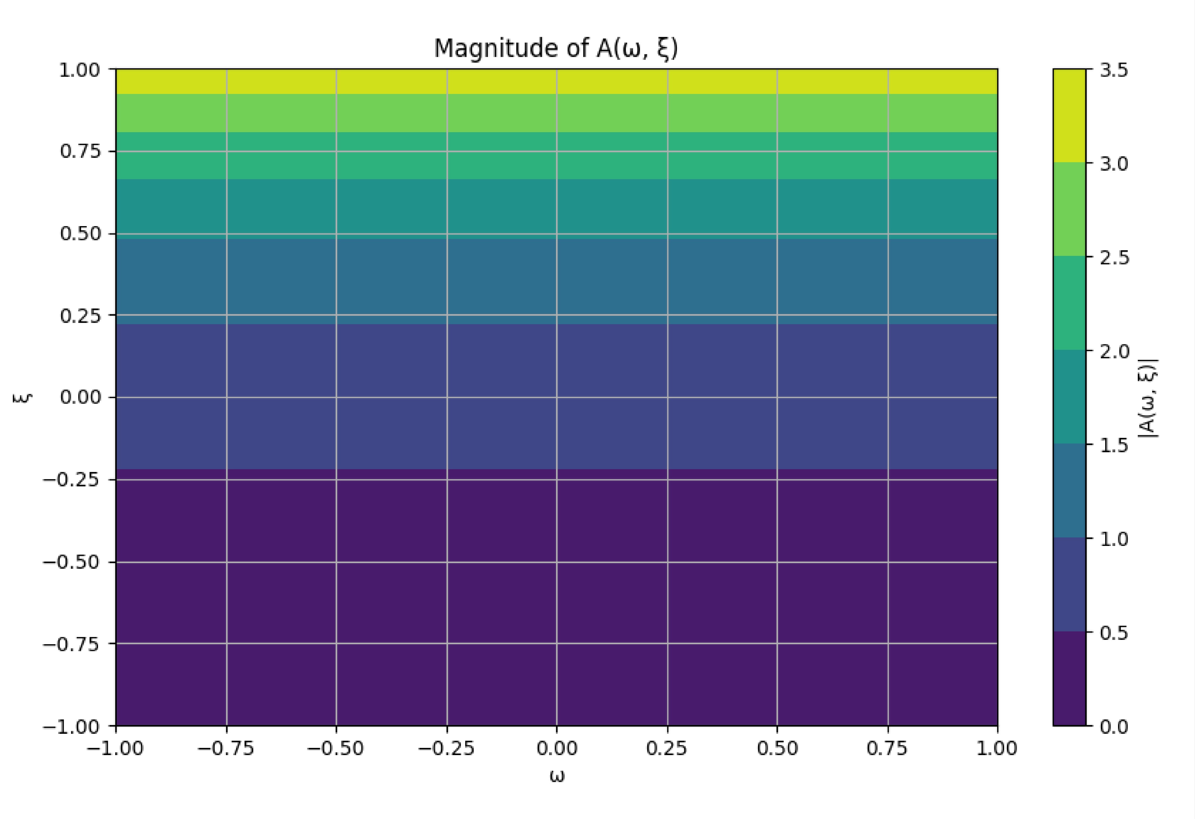
Figure 1: The plot shows how the gauge field $A_{\mathbf{+}}$ changes with respect to $\left(\omega,\xi\right)$. Parametersare defined. as $z=k=\tau=1$ and $\tau_{0}=1.$

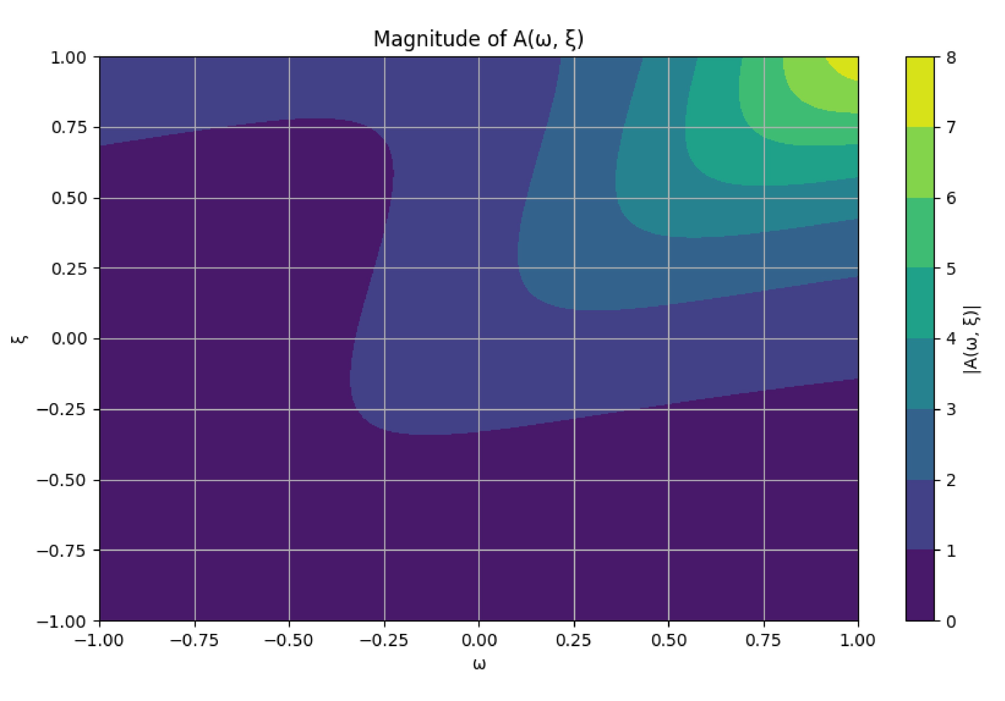
Figure 2: The plot shows how the gauge field $A_{\mathbf{+}}$ changes with respect to $\left(\omega,\xi\right)$. Parametersare defined. as $z=k=\tau=1$ and $\tau_{0}=1.5$.

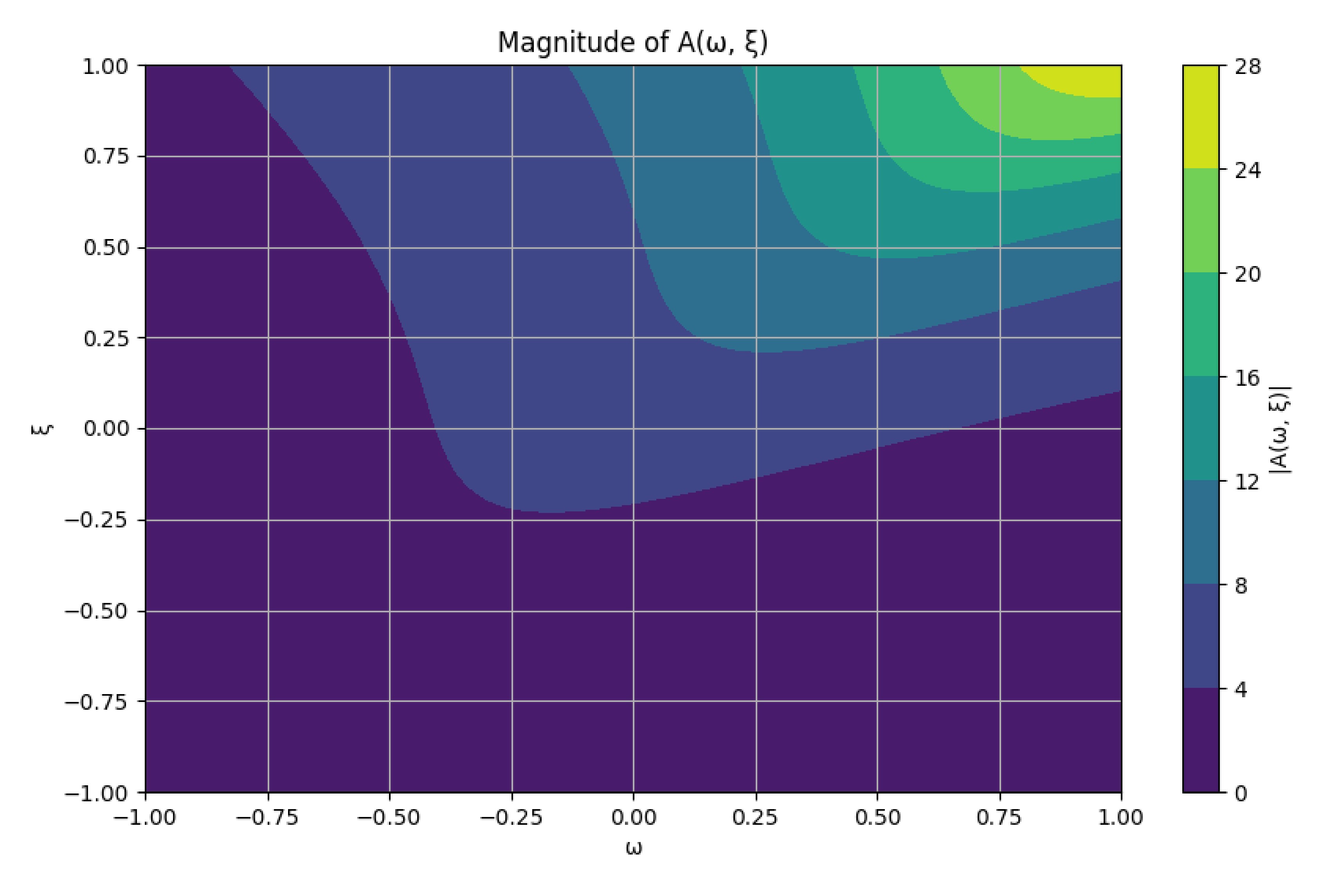
Figure 3: The plot shows how the gauge field $A_{\mathbf{+}}$ changes with respect to $\left(\omega,\xi\right)$. Parametersare defined. as $z=k=\tau=1$ and $\tau_{0}=3$.

We generate a grid of $\omega$ and $\xi$ values to compute $A_{\mathbf{+}}$ over an interval in Fig. 1. As shown in Figs. (1)-(2), the parameter $\tau_{0}$ is crucial for describing how $A_{\mathbf{+}}$ changes. Moreover, the diagram in Fig. (3) not only shows the case for $\tau_{0}=3$, but also illustrates how $A_{\mathbf{+}}$ evolves for all other values of $\tau_{0}\geq 3$. The goal of this study is to examine how the mass of the gauge field $m_{A}\sim\omega$ affects the Hubble parameter $H\sim\frac{1}{\xi}$. Perhaps the discrepancy in the measurements of the universe’s expansion rate, known as the Hubble tension [27, 28, 29], is related to how the Hubble parameter $H$ depends on the mass of the gauge bosons in the early universe. The value of $\tau_{0}=3$ signifies the critical point at which the mass of the gauge boson begins to affect the Hubble parameter. This effect is primarily due to the space-time curvature induced by these massive bosons.

Hopf fibration. In the study [26], they showed the existence of gravitational type gravitational hopfions. Likewise, we will consider that the additional term $M_{\mp i\xi,-i\omega}$ which is added to $A_{\mathbf{\pm}}$ describes the hopfions in the early universe. In this section, our objective is to demonstrate the presence of hopfions in the early universe. The average energy density of the gauge field $A_{\mu}$ can be written as $\rho_{A}=\frac{1}{2}\left\langle\mathbf{E}^{2}+\mathbf{B}^{2}+\frac{m_{A}^{2}}{a^{2}}\mathbf{A}^{2}\right\rangle.$ We express the term $\mathbf{E\cdot B}$ in the form given by [24]

$$\left\langle\mathbf{E\cdot B}\right\rangle=-\frac{1}{a^{4}}\int\frac{d^{3}k}{\left(2\pi\right)^{3}}\frac{k}{2}\frac{d}{d\tau}\left(\left|A_{\mathbf{+}}\right|^{2}-\left|A_{\mathbf{-}}\right|^{2}\right).$$ (14)

Next, we introduce the conjugate term:

$$\left\langle\mathbf{E\cdot B}\right\rangle^{\ast}\equiv-\frac{1}{a^{4}}\int\frac{d^{3}k}{\left(2\pi\right)^{3}}\frac{k}{2}\frac{d}{d\tau}\left(2A_{\mathbf{+}}A_{\mathbf{-}}^{\ast}\right).$$ (15)

The spherically equivariant map to compactifiy $\mathbb{R}^{3}\rightarrow S_{A_{\mathbf{+}},A_{\mathbf{-}}}^{3}\subset\mathbb{C}^{2}$ is

$$S_{A_{\mathbf{+}},A_{\mathbf{-}}}^{3}\cong\left\{\left(A_{\mathbf{+}}A_{\mathbf{-}}\right)\in\mathbb{C}^{2},\left|A_{\mathbf{+}}\right|^{2}+\left|A_{\mathbf{-}}\right|^{2}=1\right\},$$ (16)

where $S_{A_{\mathbf{+}},A_{\mathbf{-}}}^{3}\simeq SU(2)$. The Hopf fibration $\mathbf{P}_{h}$ is then defined as [30, 31, 32]

$$\mathbf{P}_{h}\left(A_{\mathbf{+}},A_{\mathbf{-}}\right)=\left(2A_{\mathbf{+}}A_{\mathbf{-}}^{\ast},\left|A_{\mathbf{+}}\right|^{2}-\left|A_{\mathbf{-}}\right|^{2}\right),$$ (17)

which satisfies $\frac{d\mathbf{P}_{h}\left(A_{\mathbf{+}},A_{\mathbf{-}}\right)}{d\tau}=-3\left(2\pi\right)^{3}\left(\frac{2a}{k}\right)^{4}\left(\left\langle\mathbf{E\cdot B}\right\rangle^{\ast},\left\langle\mathbf{E\cdot B}\right\rangle\right).$ The Hopf index $\mathcal{H}$ emerges as the most appropriate topological invariant for characterizing these phenomena

$$\mathcal{H}=\frac{1}{\left(8\pi\right)^{2}}\int d^{3}x\mathbf{A\cdot B.}$$ (18)

The spacetime Hopf index $\mathcal{H}$ emerges as the most appropriate topological invariant for characterizing these phenomena $\frac{d\mathcal{H}}{d\tau}=-\frac{\pi a^{2}}{\left(2\pi\right)^{3}}\int d^{3}x\mathbf{E\cdot B-}\frac{\pi a}{\left(2\pi\right)^{3}}\int d^{3}x\mathbf{A\cdot}\nabla\times\mathbf{E,}$ where $\frac{\partial\mathbf{B}}{\partial t}=\frac{\partial\mathbf{B}}{a\partial\tau}=-\nabla\times\mathbf{E}$. This perturbation can be expressed as

$$\frac{d\mathcal{H}}{d\tau}\mathbf{\approx}-\frac{\pi a^{2}}{\left(2\pi\right)^{3}}\int d^{3}x\left\langle\mathbf{E\cdot B}\right\rangle.$$ (19)

Substituting Eq. (14) into Eq. (19), we ascertain that

$$\frac{d\mathcal{H}}{d\tau}\mathbf{=}\frac{\pi}{2\left(2\pi\right)^{3}a^{2}}\int d^{3}x\int\frac{d^{3}k}{\left(2\pi\right)^{3}}k\frac{d}{d\tau}\left(\left|A_{\mathbf{+}}\right|^{2}-\left|A_{\mathbf{-}}\right|^{2}\right)e^{ikx}e^{-ikx},$$

or equivalently

$$\frac{d\mathcal{H}}{d\tau}\mathbf{=}\frac{\pi k}{2\left(2\pi\right)^{3}a^{2}}\frac{d}{d\tau}\left(\left|A_{\mathbf{+}}\right|^{2}-\left|A_{\mathbf{-}}\right|^{2}\right).$$ (20)

Subsequently we assume that $a^{2}=\frac{\pi k}{2\left(2\pi\right)^{3}}$ and we find

$$\mathcal{H}\mathbf{=}\left|A_{\mathbf{+}}\right|^{2}-\left|A_{\mathbf{-}}\right|^{2}.$$ (21)

The terms $\left|A_{\mathbf{+}}\right|$ and $\left|A_{\mathbf{-}}\right|^{2}$ can be linked to energy or load density associated with these fields. From this relationship we notice for $\mathcal{H}=0$, the magnitudes of $\left|A_{\mathbf{+}}\right|$ and $\left|A_{\mathbf{-}}\right|$ are equal. On the other hand we can calculate the conjugate of $\mathcal{H}$ as follows

$$\frac{d\mathcal{H}^{\ast}}{d\tau}=-\frac{\pi a^{2}}{\left(2\pi\right)^{3}}\int d^{3}x\left\langle\mathbf{E\cdot B}\right\rangle^{\ast}.$$ (22)

Replacing the expression from Eq. (15) into Eq. (22), we establish that

$$\frac{d\mathcal{H}^{\ast}}{d\tau}=\frac{\pi k}{2a^{2}\left(2\pi\right)^{3}}\frac{d}{d\tau}\left(2A_{\mathbf{+}}A_{\mathbf{-}}^{\ast}\right).$$

Setting $a^{2}=\frac{\pi k}{2\left(2\pi\right)^{3}}$, we derive that

$$\mathcal{H}^{\ast}=2A_{\mathbf{+}}A_{\mathbf{-}}^{\ast}.$$ (23)

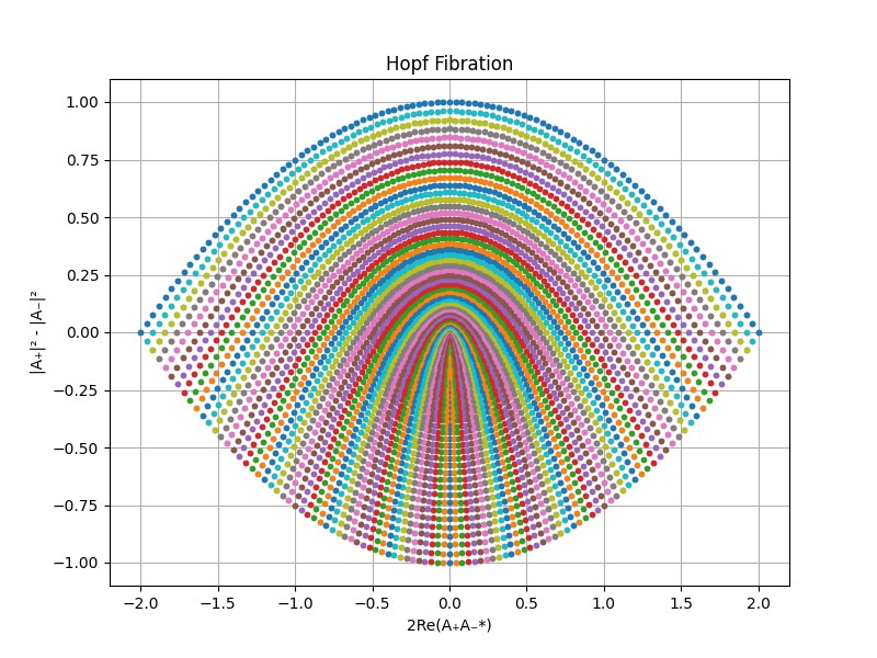
Figure 4: This figure represents the Hopf fibration $\mathbf{P}_{h}$ about the gauge field modes $A_{\mathbf{+}}$ and $A_{\mathbf{-}}$. Each point on the plot signifies the outcome of the Hopf fibration for a specific pair of $A_{\mathbf{+}}$ and $A_{\mathbf{-}}$ values.

Fig. (4) illustrates the outcome of our research, demonstrating that the massive gauge field can produce a Hopf fibration, representing regions in space-time where Hopfions are applicable. These Hopfions encompass points that form lines, adhering to the space-time curvature induced by the mass $m_{A}$. From Eqs. (17)-(21)-(23) we get

$$\mathbf{P}_{h}\left(A_{\mathbf{+}},A_{\mathbf{-}}\right)=\left(\mathcal{H}^{\ast},\mathcal{H}\right).$$ (24)

We have shown that the Hopf fibration is articulated through the presence of two Hopf index components Fig. (4). This revelation enables the characterization of the Hopfion state in the early universe. Following the inflationary epoch characterized by the inflation field, the radiation era begins, orchestrated by the electromagnetic field. However, the emergence of topological defects in spacetime, specifically hopfions, occurs during this phase. Within these regions, novel fluctuations manifest, potentially serving as the source of the pulsar timing arrays signal [33, 34, 35, 36]. On the other hand, the $\mathbf{P}_{h}\left(A_{\mathbf{+}},A_{\mathbf{-}}\right)$ resides on the unit 2-sphere in $\mathbb{C}\times\mathbb{R}$. Conclusion. This study introduces a new method for examining the dynamics of inflation fields in conjunction with a massive gauge boson. We developed a new model that characterizes the curvature of space-time, influenced by a massive gauge field in the early universe. This curvature can lead to numerous observations, such as the Hubble tension issue and the isotropic stochastic gravitational-wave background. To address this, we are introducing the concept of gauge field Hopfions. The solution for the gauge field is represented by the Whittaker function. This framework allows for the direct determination of the relationships between the mode functions of the gauge field $A_{\mathbf{\pm}}$, the Hubble parameter $H$, and the mass of the gauge field $m_{A}$. Additionally, our results show a significant correlation between the Hubble parameter and the mass $m_{A}$, as shown in the curves Figs. (1)-(2)-(3), which illustrate that the parameter $\tau_{0}$ is crucial for determining the variation of mode $A_{\mathbf{+}}$. This correlation could potentially offer a comprehensive explanation for the Hubble tension. Moreover, Fig. (3) presents the case for $\tau_{0}=3$ and also the evolution of mode $A_{\mathbf{+}}$ for all other values of $\tau\geq 3$. The goal of this research is to investigate how the Hubble parameter is affected by the mass of the gauge field. Furthermore, we have shown that the mode functions of the gauge field can be expressed within the context of a component of the Hopf fibration. After our calculations, we confirmed the accuracy of this proposition by demonstrating that the Hopf fibration of the gauge field is articulated in terms of the Hopf index $\mathcal{H}$ and their combination. We have demonstrated that the Hopf fibration is expressed via the existence of two components of the Hopf index as shown in Fig. (4). This discovery allows for the description of the Hopfion state in the early universe. After the inflationary period defined by the inflation field, the era of radiation begins, governed by the electromagnetic field. However, during this phase, topological defects in space-time, particularly hopfions, emerge. Within these areas, new fluctuations appear, which could potentially be the origin of the pulsar timing arrays.

References

[1] Maleknejad, A., & Sheikh-Jabbari, M. M. (2011), Physical
Review D, 84(4), 043515.
[2] Maleknejad, A., & Sheikh-Jabbari, M. (2013), Physics Letters
B, 723(1-3), 224-228.
[3] Guth, A. H. (1981), Physical Review D, 23(2), 347.
[4] Linde, A. D. (1982), Physics Letters B, 108(6), 389-393.
[5] Maleknejad, A., Sheikh-Jabbari, M. M., & Soda, J. (2013),
Physics Reports, 528(4), 161-261.
[6] Adshead, P., Martinec, E., & Wyman, M. (2013), Physical
Review D, 88(2), 021302.
[7] Agrawal, A., Fujita, T., & Komatsu, E. (2018), Physical
Review D, 97(10), 103526.
[8] Agrawal, A., Fujita, T., & Komatsu, E. (2018), Journal of
Cosmology and Astroparticle Physics, 2018(06), 027.
[9] Alexander, S. H., Peskin, M. E., & Sheikh-Jabbari, M. M.
(2006), Physical Review Letters, 96(8), 081301.
[10] Corianò, C., Lionetti, S., & Maglio, M. M. (2024),
Physical Review D, 109(4), 045004.
[11] Prokhorov, G. Y., Teryaev, O. V., & Zakharov, V. I. (2023),
Physics Letters B, 840, 137839.
[12] Cook, J. L., & Sorbo, L. (2012), Physical Review D, 85(2),
023534.
[14] Niu, X., Rahat, M. H., Srinivasan, K., & Xue, W. (2023).
Journal of Cosmology and Astroparticle Physics, 2023(02), 013.
[15] Kent, N., Reynolds, N., Raftrey, D., Campbell, I. T.,
Virasawmy, S., Dhuey, S., … & Fischer, P. (2021), Nature communications,
12(1), 1562.
[16] Wang, X. S., Qaiumzadeh, A., & Brataas, A. (2019), Physical
Review Letters, 123(14), 147203.
[17] Sutcliffe, P. (2018), Journal of Physics A: Mathematical and
Theoretical, 51(37), 375401.
[18] Raftrey, D., & Fischer, P. (2021), Field-driven dynamics of
magnetic hopfions. Physical Review Letters, 127(25), 257201.
[19] Liu, Y., Watanabe, H., & Nagaosa, N. (2022). Emergent
magnetomultipoles and nonlinear responses of a magnetic hopfion. Physical
Review Letters, 129(26), 267201.
[20] Wang, H., & Fan, S. (2023). Photonic Spin Hopfions and
Monopole Loops. Physical Review Letters, 131(26), 263801.
[21] Liu, Y., Hou, W., Han, X., & Zang, J. (2020).
Three-dimensional dynamics of a magnetic hopfion driven by spin transfer
torque. Physical review letters, 124(12), 127204.
[22] Saji, C., Troncoso, R. E., Carvalho-Santos, V. L., Altbir,
D., & Nunez, A. S. (2023). Hopfion-Driven Magnonic Hall Effect and Magnonic
Focusing. Physical Review Letters, 131(16), 166702.
[23] Niu, X., & Rahat, M. H. (2023), Physical Review D, 108(11),
115023.
[24] Fujita, T., Namba, R., Tada, Y., Takeda, N., & Tashiro, H.
(2015). Journal of Cosmology and Astroparticle Physics, 2015(05), 054.
[25] Kuroyanagi, S., Chiba, T., and Takahashi, T., 2018, Journal
of Cosmology and Astroparticle Physics, 2018(11), 038.
[26] Swearngin, J., Thompson, A., Wickes, A., Dalhuisen, J. W., &
Bouwmeester, D. (2013), arXiv preprint arXiv:1302.1431.
[27] Di Valentino, E., Mena, O., Pan, S., Visinelli, L., Yang, W.,
Melchiorri, A., … & Silk, J. (2021), Classical and Quantum Gravity,
38(15), 153001.
[28] Poulin, V., Smith, T. L., Karwal, T., & Kamionkowski, M.
(2019), Physical Review Letters, 122(22), 221301.
[29] Feeney, S. M., Peiris, H. V., Williamson, A. R., Nissanke, S.
M., Mortlock, D. J., Alsing, J., & Scolnic, D. (2019), Physical Review
Letters, 122(6), 061105.
[30] Lyons, D. W. (2003). Mathematics magazine, 76(2), 87-98.
[31] Urbantke, H. K. (2003). Journal of geometry and physics,
46(2), 125-150.
[32] Roa, J., Urrutxua, H., & Peláez, J. (2016). Monthly
Notices of the Royal Astronomical Society, 459(3), 2444-2454.
[33] Afzal, A., et al. and NANOGrav Collaboration, 2023, The
Astrophysical Journal Letters, 951(1), L11.
[34] G. Agazie et al. and NANOGrav Collaboration, 2023, The
Astrophysical Journal Letters, 951(1), L8.
[35] Arzoumanian, Z., et al. and NANOGrav Collaboration, 2020,
The Astrophysical Journal Letters, 905(2), L34.
[36] Arzoumanian, Z., et al. and NANOGrav Collaboration, 2021,
Physical Review Letters, 127(25), 251302.