Dirac and Majorana Fermions in the Anti-de Sitter spacetime with Tachyonic approaches

Abstract

We analyze the Dirac equation in Anti-de Sitter (AdS) spacetime upon the comformally flat spacetime. We also apply the analysis to the Majorana condition. The analytical solutions are neat. We observe that Dirac fermions and Majorana fermions behave differently in AdS background. The wavefunction of tachyonic neutrinos leaves an track, clumping in a special flatland, embedded in the curved 3+1-D AdS spacetime. Besides, there emerges a boundary, and neutrinos also oscillate.

.

I Introduction

The task to find solutions of Dirac equations in curved spacetime relies on decoupling the equations, especially in curved spacetime. The well-known examples of Dirac equations in Kerr geometry and de Sitter spacetime can be seen from Chandrasekhar[1] and Dirac[2]. In this paper, we will study the Dirac equation in Anti-de Sitter (AdS) spacetime. Instead of going directly to the curved spacetime [3], we take advantage of the conformally flat coordinate in AdS spacetime, which is rarely discussed. Then with Newman-Penrose (NP) formalism [4] and tricks in section II, we decouple the equations neatly and have profound results.

Physically, AdS spacetime is a solution of Einstein’s field equation with a negative constant $\Lambda$, giving an attracting geometry. And the metric can be read as $ds^{2}=(1+\frac{\Lambda}{3}r^{2})d\bar{t}^{2}-\frac{dr^{2}}{1+\frac{\Lambda}{3}r^{2}}-r^{2}(d\theta^{2}+\sin^{2}\theta d\phi^{2})$, with cosmological constant $\Lambda$. We can transform it into a conformally flat spacetime without changing physical meaning (just seen from another frame)

$$ds^{2}=\frac{1}{z^{2}}(dt^{2}-dz^{2}-dx^{2}-dy^{2})$$ (1)

by the recipe[5]

$$\begin{split}&\sqrt{r^{2}+a^{2}}\cos\bar{t}=\frac{1}{2z}(a^{2}+x^{2}+y^{2}+z^{2}-t^{2})\\ &\sqrt{r^{2}+a^{2}}\sin\bar{t}=\frac{at}{z}\\ &r\sin\theta\cos\phi=\frac{ax}{z}\\ &-r\sin\theta\sin\phi=\frac{ay}{z}\\ &-r\cos\theta=\frac{1}{2z}(-a^{2}+x^{2}+y^{2}+z^{2}-t^{2}),\end{split}$$ (2)

where $a^{2}=\frac{3}{|\Lambda|}$ and the $\Lambda$ is absorbed. Alternatively, the AdS metric (1) can be obtained as a result of reflecting null-shells from a boundary [6]. we can see that for constant z the AdS spacetime can be reduced to a $2+1-D$ flat spacetime, that is, every slice of constant z corresponds to a lower/flat spacetime.

In addition to solving the Dirac equations, a wavefunction of tachyon is also introduced. We resemble the wavefunctions as neutrinos, which inspires some interesting phenomena. Besides, we also derive the Majorana fermions in the AdS spacetime. Since gravity distinguishes Dirac and Majorana particles [7], then, we may ask the question: Can the attractive AdS geometry also distinguish between Dirac and Majorana?

Our paper is organized as follows. In section II, we discuss the differential equations and derive the wavefunctions and the boundary. We consider the tachyonic fields in the AdS background in section III. In Section IV, th Majorana condition is imposed. We complete the paper with our discussion and conclusion in section V.

II The Method

Consider the Dirac equation in AdS spacetime by using the Newman-Penrose (NP) formalism [4] refering to Chandrasekhar [1].

$$\begin{split}&(D+\epsilon-\rho)F_{1}+(\bar{\delta}+\pi-\alpha)F_{2}=imG_{1}\\ &(\Delta+\mu-\gamma)F_{2}+(\delta+\beta-\tau)F_{1}=imG_{2}\\ &(D+\bar{\epsilon}-\bar{\rho})G_{2}-(\delta+\bar{\pi}-\bar{\alpha})G_{1}=imF_{2}\\ &(\Delta+\bar{\mu}-\bar{\gamma})G_{1}-(\bar{\delta}+\bar{\beta}-\bar{\tau})G_{2}=imF_{1},\end{split}$$ (3)

where $\alpha,\beta,\gamma,\rho,\epsilon,\mu,\pi,\tau$ are spin coefficients, $D,\Delta,\delta$, the directional derivatives, m the mass and $F_{1},F_{2},G_{1},G_{2}$ the spinor components. From the Eqn (1), we may choose the null tetrad basis 1-forms as

$$\begin{split}&\sqrt{2}l=\frac{1}{z}(dt-dz)\\ &\sqrt{2}n=\frac{1}{z}(dt+dz)\\ &\sqrt{2}m=\frac{1}{z}(dx+idy)\\ &\sqrt{2}\bar{m}=\frac{1}{z}(dx-idy),\end{split}$$ (4)

which gives us the only non-zero spin coefficients $\epsilon=\gamma=-\frac{1}{2\sqrt{2}},\mu=\rho=\frac{1}{\sqrt{2}}$ ,Ricci scalar $R=-12$ and the directional derivatives

$$\begin{split}&D=\frac{z}{\sqrt{2}}(\partial_{t}+\partial_{z})\\ &\Delta=\frac{z}{\sqrt{2}}(\partial_{t}-\partial_{z})\\ &\delta=-\frac{z}{\sqrt{2}}(\partial_{x}+i\partial_{y})\\ &\bar{\delta}=-\frac{z}{\sqrt{2}}(\partial_{x}-i\partial_{y}).\end{split}$$ (5)

Therefore, we have the Dirac equations

$$\begin{split}&(D-\frac{3}{2\sqrt{2}})F_{1}+\bar{\delta}F_{2}=imG_{1}\\ &(\Delta+\frac{3}{2\sqrt{2}})F_{2}+\delta F_{1}=imG_{2}\\ &(D-\frac{3}{2\sqrt{2}})G_{2}-\delta G_{1}=imF_{2}\\ &(\Delta+\frac{3}{2\sqrt{2}})G_{1}-\bar{\delta}G_{2}=imF_{1}.\end{split}$$ (6)

To solve these equations, we consider the ansatz

$$\begin{split}&F_{i}=f_{i}(z)e^{i\omega t+ip_{1}x+ip_{2}y}\\ &G_{i}=g_{i}(z)e^{i\omega t+ip_{1}x+ip_{2}y}.\end{split}$$ (7)

Therefore, we derive

$$\begin{split}&Pf_{1}-(p_{2}+ip_{1})f_{2}=\frac{i\sqrt{2}mg_{1}}{z}\\ &\bar{P}f_{2}-(p_{2}-ip_{1})f_{1}=-\frac{i\sqrt{2}mg_{2}}{z}\\ &Pg_{2}-(p_{2}-ip_{1})g_{1}=\frac{i\sqrt{2}mf_{2}}{z}\\ &\bar{P}g_{1}-(p_{2}+ip_{1})g_{2}=-\frac{i\sqrt{2}mf_{1}}{z},\end{split}$$ (8)

with the definition of operator, $P=\partial_{z}-\frac{3}{2z}+i\omega$ and its complex conjugate $\bar{P}$. By multiplying all the equations with its complex conjugate operator, we obtain

$$\begin{split}&f^{\prime\prime}_{1}-\frac{3}{z}f^{\prime}_{1}+(\frac{15-8m^{2}}{4z^{2}}+\omega^{2}-p^{2}_{1}-p^{2}_{2})f_{1}=-\frac{i\sqrt{2}m}{z^{2}}g_{1}\\ &f^{\prime\prime}_{2}-\frac{3}{z}f^{\prime}_{2}+(\frac{15-8m^{2}}{4z^{2}}+\omega^{2}-p^{2}_{1}-p^{2}_{2})f_{2}=\frac{i\sqrt{2}m}{z^{2}}g_{2}\\ &g^{\prime\prime}_{2}-\frac{3}{z}g^{\prime}_{2}+(\frac{15-8m^{2}}{4z^{2}}+\omega^{2}-p^{2}_{1}-p^{2}_{2})g_{2}=-\frac{i\sqrt{2}m}{z^{2}}f_{2}\\ &g^{\prime\prime}_{1}-\frac{3}{z}g^{\prime}_{1}+(\frac{15-8m^{2}}{4z^{2}}+\omega^{2}-p^{2}_{1}-p^{2}_{2})g_{1}=\frac{i\sqrt{2}m}{z^{2}}f_{1},\end{split}$$ (9)

Now consider the on-shell condition and set $\omega^{2}-p^{2}_{1}-p^{2}_{2}=p^{2}_{3}+m^{2}=k^{2}$. One observes that from the equations the choices $f_{1}=ig_{1}$ and $f_{2}=ig_{2}$ decouple the equations and the Dirac equations are in consistent with each other. To solve the Dirac equations, we consider

$$\begin{split}&f_{1}=A+iB\\ &f_{2}=C+iD\\ &g_{1}=E+iF\\ &g_{2}=G+iH\\ \end{split}$$ (10)

where A, B,… are real functions and set $\Box f=f^{\prime\prime}-\frac{3}{z}f^{\prime}+(\frac{15-8m^{2}}{4z^{2}}+k^{2})f$. We then derive

$$\begin{split}&\Box A=\frac{\sqrt{2}m}{z^{2}}F,\Box B=-\frac{\sqrt{2}m}{z^{2}}E\\ &\Box C=-\frac{\sqrt{2}m}{z^{2}}H,\Box D=\frac{\sqrt{2}m}{z^{2}}G\\ &\Box G=\frac{\sqrt{2}m}{z^{2}}D,\Box H=-\frac{\sqrt{2}m}{z^{2}}C\\ &\Box E=-\frac{\sqrt{2}m}{z^{2}}B,\Box F=\frac{\sqrt{2}m}{z^{2}}A.\\ \end{split}$$ (11)

Equation (11) plays the crucial to get the consistent Dirac equaitons. However, to decouple the equations, one may choose

$$\begin{split}&A=-F,C=-H\\ &B=E,D=G.\\ \end{split}$$ (12)

Thus,

$$\begin{split}&f_{1}=A+iB,f_{2}=C+iD\\ &g_{1}=B-iA,g_{2}=D-iC,\\ \end{split}$$ (13)

and $f_{1}=ig_{1}$, $f_{2}=ig_{2}$ are satisfied. The equation (11) should be reduced to $\Box A=\frac{\sqrt{2}m}{z^{2}}A$, $\Box B=-\frac{\sqrt{2}m}{z^{2}}B$ or

$$\begin{split}&A^{\prime\prime}-\frac{3}{z}A^{\prime}+(\frac{15-8m^{2}-4\sqrt{2}m}{4z^{2}}+k^{2})A=0\\ &B^{\prime\prime}-\frac{3}{z}B^{\prime}+(\frac{15-8m^{2}+4\sqrt{2}m}{4z^{2}}+k^{2})B=0.\\ \end{split}$$ (14)

To solve A and B, we refer to Lommel [8] that

$$z^{2}f^{\prime\prime}+(2\alpha-2\beta\nu+1)zf^{\prime}+[\alpha(\alpha-2\beta\nu)+\beta^{2}\gamma^{2}z^{2\beta}]f=0$$ (15)

with a solution

$$f=z^{\beta\nu-\alpha}[a_{0}J_{\nu}(\gamma z^{\beta})+b_{0}J_{-\nu}(\gamma z^{\beta})],$$ (16)

where $a_{0}$ and $b_{0}$ are constants. Therefore,

$$A(z)=z^{2}[a_{0}J_{\nu}(kz)+b_{0}J_{-\nu}(kz)],$$ (17)

where $\nu=\pm\sqrt{\frac{1}{4}+\sqrt{2}m(\sqrt{2}m+1)}$, and

$$B(z)=z^{2}[c_{0}J_{\nu}(kz)+d_{0}J_{-\nu}(kz)]$$ (18)

with $\nu=\pm\sqrt{\frac{1}{4}+\sqrt{2}m(\sqrt{2}m-1)}$ and ($c_{0},d_{0}$) constants. For massless case, $\nu=\pm\frac{1}{2}$, we got $z^{2}J_{\pm\frac{1}{2}}$. The Bessel function performs as a periodic function with decay. We may consider that asymptotic approach, $z>>1$, the differential equation reduces to

$$f^{\prime\prime}-\frac{3}{z}f^{\prime}+k^{2}f=0,$$ (19)

which gives a neat solution, $z^{2}J_{2}(kz)$ or $z^{2}N_{2}(kz)$, where $N(kz)$ is the Neumann function. Therefore, from our ansatz (7), we can build the spinor.

In the kinetic energy dominated regime, $k>>1$ , we can see from the differential equations that

$$f^{\prime\prime}+k^{2}f\approx 0,$$ (20)

which brings us the solution, $f=A_{0}sin(kz)+B_{0}cos(kz)$. One may regard these solutions as neutrino because we cannot bring it to rest. For simplicity, we let 2 mass states to be

$$\begin{split}&f_{\nu 1}=A_{0}sin(k_{1}z)\\ &f_{\nu 2}=A_{0}sin(k_{2}z),\end{split}$$ (21)

where $k_{1}=\sqrt{p^{2}_{3}+m^{2}_{1}}\approx p_{3}+\frac{m^{2}_{1}}{2p_{3}}$ and $k_{2}\approx p_{3}+\frac{m^{2}_{2}}{2p_{3}}$. Set $k=\frac{k_{1}+k_{2}}{2}$ and $\Delta k=\frac{m^{2}_{1}-m^{2}_{2}}{4p_{3}}$, then $k_{1}=k+\Delta k$ and $k_{2}=k-\Delta k$. The combination of neutrinos becomes

$$\nu_{1}+\nu_{2}=2A_{0}sin(kz)cos(\Delta kz).$$ (22)

The simple version of neutrino beat or neutrino oscillation is recovered in the AdS background.

The AdS spacetime is an attractive geometry as it is well-known from AdS/CFT correspondence [9]. Particles tend to deviate inward. We can observe that $z^{2}$ accompanies all the Bessel functions, which makes all the wavefunctions become zero as $z\to$ 0. There emerges a boundary at $z=0$. In this way all the information would be lost in the boundary, the wavefunction would disappear. However, after examining the geodesic (in the Appendix), we find that the wavefunction can only diminish and fall into a $z=z_{0}$ plane. We may choose the $\xi$ to be very large, so that $z_{0}=\frac{1}{\xi}$ would be in the edge of boundary $z=0$ (in the Appendix). Therefore, $z^{2}_{0}J(kz_{0})$ becomes constant, the other components still propagate in the $z_{0}$ plane, the $2+1-D$ lower and flat spacetime, see Figure 1. As a result, we find that higher dimension may collapse into lower dimension and the wavefunctions are special signals to mediate between higher and lower dimensions in the AdS geometry,.

III Tachyonic condition

The equation of motion includes not only usual Dirac fermions but tachyons. The motivation comes from Chodos [10] that neutrinos may be in the tachyonic form. Therefore, in this section we assume the tachyonic condition, that is,

$$\omega^{2}-p^{2}_{1}-p^{2}_{2}=p^{2}_{3}+m^{2}=-\kappa^{2}.$$ (23)

Obviously, $p^{2}_{3}>0$. So $m$ has to be replaced by $im$ for $\kappa^{2}>0$. The equations of motion now become

$$\begin{split}&\bar{\Box}f_{1}=\frac{\sqrt{2}m}{z^{2}}g_{1},\bar{\Box}f_{2}=-\frac{\sqrt{2}m}{z^{2}}g_{2}\\ &\bar{\Box}g_{1}=-\frac{\sqrt{2}m}{z^{2}}f_{1},\bar{\Box}g_{2}=\frac{\sqrt{2}m}{z^{2}}f_{2}\\ ,\end{split}$$ (24)

where $\bar{\Box}f=f^{\prime\prime}-\frac{3}{z}f^{\prime}+(\frac{15+8m^{2}}{4z^{2}}-\kappa^{2})f$. The condition $f_{1}=ig_{1}$, $f_{2}=ig_{2}$ also applies here, but the function can not be decomposed into real and imaginary part easily. We have to directly solve equations

$$\bar{\Box}f_{1}=-i\frac{\sqrt{2}m}{z^{2}}f_{1},\bar{\Box}f_{2}=i\frac{\sqrt{2}m}{z^{2}}f_{2},$$ (25)

The solutions are $z^{2}K_{\nu}(\kappa z)$, where $K_{\nu}(\kappa z)$ is modified Bessel function, and $\nu=\frac{1}{2}-i\sqrt{2}m$ for $f_{1}$, and $\nu={\frac{1}{2}+i\sqrt{2}m}$ for $f_{2}$.

If the neutrinos are tachyons [10], we see that the index $\nu=\frac{1}{2}$ dominates the modified Bessel function due to negligible mass of neutrinos. As one can see from Figure 2, before the wavefunction diminishes to the boundary, it has a higher chance to be seen at constant slice $z_{d}$. The particles here are fermions, therefore they are more likely to clump in a $z=z_{d}$ slice, that is, a $2+1-D$ spacetime. There arises a phenomenon: In AdS spacetime, we have found a special shell that all 3 types of neutrinos inhabit. In other words, we find a ”Flatland” for neutrinos, since the shell is a $2+1-D$ flat spacetime. It is important to find a flat frame embedded in the curved spacetime. Thus, in curved AdS background, there may exist a flat shell, and in this shell, one could discuss the propagation with no curvature effects.

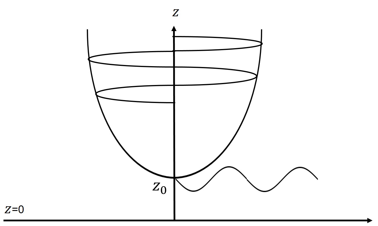
Figure 1: The $3+1-D$ wavefunction diminishes and collapses into a $2+1-D$ plane wave at $z=z_{0}$.

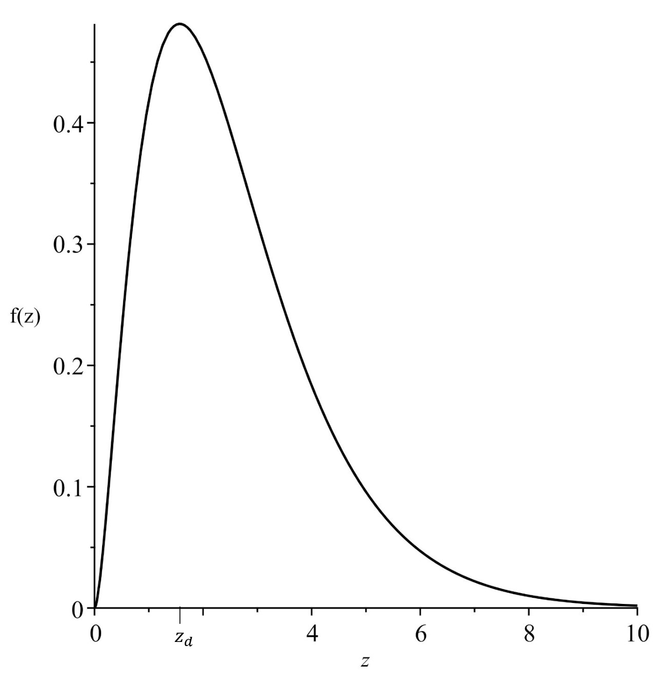
Figure 2: The wavefunction of tachyon has a maximum at $z=z_{d}$.

IV Majorana condition

In Dirac equations, we may impose the Majorana condition [11],

$$\Psi_{M}=\begin{bmatrix}\phi\\ i\sigma_{2}\phi^{*}\end{bmatrix},$$ (26)

such that $\Psi_{M}$ would be its own antiparticle, where $\sigma_{2}=\begin{bmatrix}0&-i\\ i&0\end{bmatrix}$. Set $\phi=\begin{bmatrix}A\\ B\end{bmatrix}$.

$$\therefore\Psi_{M}=\begin{bmatrix}A\\ B\\ B^{*}\\ -A^{*}\end{bmatrix}.$$ (27)

Comparing Chandrasekhar’s assumption [1] with the Majorana condition leads to

$$\begin{bmatrix}P^{A}\\ \bar{Q}^{A^{\prime}}\end{bmatrix}=\begin{bmatrix}P^{0}\\ P^{1}\\ \bar{Q}^{0^{\prime}}\\ \bar{Q}^{1^{\prime}}\end{bmatrix}=\begin{bmatrix}F_{1}\\ F_{2}\\ -G_{2}\\ G_{1}\end{bmatrix}=\begin{bmatrix}A\\ B\\ B^{*}\\ -A^{*}.\end{bmatrix}$$ (28)

In the equation, $A\rightarrow F_{1},B\rightarrow F_{2},B^{*}\rightarrow-G_{2},-A^{*}\rightarrow G_{1}$, we therefore find the Majorana condition for Dirac equation in AdS spacetime,

$$F_{1}=-G_{1}^{*},F_{2}=-G_{2}^{*}.$$ (29)

Since the fields are Majorana, we may suggest that each component is complex conjugate to itself,

$$F_{i}=F_{i}^{*},G_{i}=G_{i}^{*}$$ (30)

and cast the ansatz as

$$\begin{split}&F_{i}=f_{i}(z)e^{-\omega t-p_{1}x-p_{2}y}\\ &G_{i}=g_{i}(z)e^{-\omega t-p_{1}x-p_{2}y}.\end{split}$$ (31)

Bringing (31) into (3) gives

$$\begin{split}&Mf_{1}+(p_{1}-ip_{2})f_{2}=\frac{i\sqrt{2}mg_{1}}{z}\\ &\bar{M}f_{2}+(p_{1}+ip_{2})f_{1}=\frac{i\sqrt{2}mg_{2}}{z}\\ &Mg_{2}+(-p_{1}-ip_{2})g_{1}=\frac{i\sqrt{2}mf_{2}}{z}\\ &\bar{M}g_{1}+(-p_{1}+ip_{2})g_{2}=\frac{i\sqrt{2}mf_{1}}{z},\end{split}$$ (32)

where we define $M=-\omega+\partial_{z}-\frac{3}{2z}$ and $\bar{M}=-\omega-\partial_{z}-\frac{3}{2z}$, and multiply $M$ and $\bar{M}$ for each as we did previously. The differential equations read

$$\begin{split}&f^{\prime\prime}_{1}-\frac{3\omega}{z}f_{1}-(\frac{3+8m^{2}}{4z^{2}}+k^{2})f_{1}=\frac{i\sqrt{2}m}{z^{2}}g_{1}\\ &f^{\prime\prime}_{2}-\frac{3\omega}{z}f_{2}-(\frac{15+8m^{2}}{4z^{2}}+k^{2})f_{2}=\frac{i\sqrt{2}m}{z^{2}}g_{2}\\ &g^{\prime\prime}_{1}-\frac{3\omega}{z}g_{1}-(\frac{15+8m^{2}}{4z^{2}}+k^{2})g_{1}=\frac{i\sqrt{2}m}{z^{2}}f_{1}\\ &g^{\prime\prime}_{2}-\frac{3\omega}{z}g_{2}-(\frac{3+8m^{2}}{4z^{2}}+k^{2})g_{2}=\frac{i\sqrt{2}m}{z^{2}}f_{2},\end{split}$$ (33)

and also the on-shell condition applies here. The difference between $f_{i}$ and $g_{i}$ are due to that $M$ and $\bar{M}$ do not commute. Then considering (29) and (30), $g_{1}\rightarrow-f_{1}^{*}\rightarrow-f_{1}$, we obtain the Whittaker equation (see [12])

$$\begin{split}f^{\prime\prime}_{1}-\frac{3\omega}{z}f_{1}-(\frac{3+8m^{2}-i4\sqrt{2}m}{4z^{2}}+k^{2})f_{1}=0\end{split},$$ (34)

and similar for the rest equations.

For heavily sterile Majorana particles in seesaw mechanism [13], $m>>1$ and $z<<1$, eqn (34) can be reduced to

$$\begin{split}f^{\prime\prime}_{1}-\frac{2m^{2}}{z^{2}}f_{1}\approx 0.\end{split}$$ (35)

The wavefunction of Majorana particles is

$$f_{1}=a_{0}e^{k_{1}\ln z}+b_{0}e^{k_{2}\ln z},$$ (36)

where $k_{1,2}=\frac{1\pm\sqrt{1+8m^{2}}}{2}$ with ($a_{0},b_{0}$) constants, and similarly for the $g_{i}$ functions but picking up a minus sign. Then $f_{i}=-g_{i}^{*}$ and $f_{i}=f_{i}^{*}$ fit the criteria of our assumptions (29) and (30).

If we loosely regard condition (29) as a boundary only involved in solving differential equations, we got some interesting results. From the ansatz (31), we may focus on $z<<1$, therefore

$$f_{1}^{{}^{\prime\prime}}-\frac{3+8m^{2}+i4\sqrt{2}m}{4z^{2}}f_{1}\approx 0.$$ (37)

We can see from the massless case, the solution is $f_{1}$ =$z^{\frac{-1}{2}}$ or $z^{\frac{3}{2}}$, and $f^{*}_{1}=f_{1}$ is satisfied. And the solution of massive case gives

$$f_{1}=e^{\frac{1}{2}(1+c+id)\ln z}+e^{\frac{1}{2}(1-c-id)\ln z},$$ (38)

where $c^{2}=\frac{1+4a\pm\sqrt{(1+4a)^{2}+16b^{2}}}{2},d=2b/c,a=\frac{3+8m^{2}}{4},b=-\sqrt{2}m$. The massive $f_{1}$ is obviously not complex conjugate to itself, unless $c=0$. However, $c=0$ implies $m=0$. To fix this, we may replace $m$ by $im$. $f_{1}$ becomes

$$f_{1}=a_{0}e^{k_{1}\ln z}+b_{0}e^{k_{2}\ln z},$$ (39)

where $k_{1,2}=\frac{1\pm\sqrt{4-8m^{2}+4\sqrt{2}m}}{2}$ with ($a_{0},b_{0}$) constants. We may choose $a_{0}=b_{0}$. Therefore, $f^{*}_{1}=f_{1}$.

We could also consider that $f_{1}$ is a wavefunction consisted of a pair of electron and hole. Then one may observe that this self-complex conjugated wavefunction evanesce or grow in z direction but with limitation, $z<<1$, if we can create a AdS-like potential in condensed matter.

V Discussion and Conclusion

We would like to promote a concept here. Spacetime like AdS can be projected to the Ginzburg-Landau theory [14]. Vice versa, quantum mechanical materials can simulate spacetime [15]. One may consider the electromagnetic interaction and gravitational effect in the derivative of the spinor $\Psi$[16, 17], $D_{\mu}\Psi=\partial_{\mu}\Psi+iq_{1}A_{\mu}\Psi+q_{2}\Gamma_{\mu}\Psi$, where $A_{\mu}$ and $\Gamma_{\mu}$ are vector potential and Riemannian connection with coupling constant $q_{1}$ and $q_{2}$, respectively. We can find a proper $A_{\mu}$ to replace $\Gamma_{\mu}$, or we can say, we mimic the non-flat space by $A_{\mu}$. Then we may try the AdS-like potential to test the wavefunction $z^{2}J_{\nu}(kz)$ of electrons and finally applying to find the Majorana particles in condensed matter [18].

By exploiting the conformally flat spacetime, we find a general form of Dirac fermions in AdS spacetime, which can be applied to free neutrinos, electrons, quarks and so on. The Majorana fermions are also discussed, and we derive the wavefunction of sterile Majorana particles. Now we can respond to the question. Can AdS geometry distinguish between Dirac and Majorana particles? Upon our calculation, we may support that Dirac and Majorana wavefunctions can be distinguished in AdS spacetime. For theoretical interest, we introduce tachyons in Dirac and Majorana equations. A ”Flatland” for tachyonic neutrinos and boundaries are naturally built. In addition, the wavefunctions we found here play the role to bridge higher and lower dimensions. Finally, we hope our finding can deepen the understanding of Dirac equations in non-flat spacetime and inspire the searching of Majorana particles as well.

Appendix

Since we have

$$ds^{2}=\frac{1}{z^{2}}(dt^{2}-dz^{2}-dx^{2}-dy^{2}),$$ (40)

the geodesic lagrangian is

$$L=\frac{1}{2z^{2}}(\dot{t}^{2}-\dot{z}^{2}-\dot{x}^{2}-\dot{y}^{2}).$$ (41)

Because x, y, and t parts are cyclic, we have

$$\begin{split}&\frac{\partial L}{\partial\dot{t}}=\frac{\dot{t}^{2}}{z^{2}}=\alpha_{0}\\ &\frac{\partial L}{\partial\dot{x}}=\frac{\dot{x}^{2}}{z^{2}}=\beta_{0}\\ &\frac{\partial L}{\partial\dot{y}}=\frac{\dot{y}^{2}}{z^{2}}=\gamma_{0},\end{split}$$ (42)

where a ’dot’ denotes derivative with respect to the proper time $\tau$. As for the z part, we should consider $1=\frac{1}{z^{2}}(\alpha_{0}^{2}z^{4}-\dot{z}^{2}-\beta_{0}^{2}z^{4}-\gamma_{0}^{2}z^{4})$, therefore

$$\dot{z}^{2}=-z^{2}+(\alpha_{0}^{2}-\beta_{0}^{2}-\gamma_{0}^{2})z^{4}=\xi^{2}z^{4}-z^{2},$$ (43)

where $\xi^{2}=\alpha_{0}^{2}-\beta_{0}^{2}-\gamma_{0}^{2}$. Also, $\frac{dz}{d\tau}=\frac{dz}{dt}\frac{dt}{d\tau}=\frac{dz}{dt}\alpha_{0}z^{2}$. As a result, $\frac{dz}{dt}=\frac{1}{\alpha_{0}}\sqrt{\frac{\xi^{2}z^{2}-1}{z^{2}}}$, and brings us

$$z=\sqrt{\frac{(t-t_{l})^{2}\xi^{2}}{\alpha_{0}^{2}}+\frac{1}{\xi^{2}}}.$$ (44)

We define the constant $t_{l}$ for life time in z-axis.

Data Availability Statement: No Data associated in the manuscript.

References

Chandrasekhar [1983]
S. Chandrasekhar, The Mathematical Theory of Black Holes, Clarendon, Oxford (1983).
Dirac [1935]
P. A. M. Dirac, Ann. Math. Vol. 36, No. 3, pp. 657-669 (1935)
Newman [1962]
E.T. Newman, and R. Penrose, Journal of Mathematical Physics, 3, 566 (1962).
Kawamoto [2022]
T. Kawamoto, T. Mori, Y.-k. Suzuki, T. Takayanagi and T. Ugajin, JHEP, 05, 060 (2022).
Halilsoy [2023]
M. Halilsoy and V.Memari, arXiv:2304.14771 (2023).
Singh [2006]
D. Singh, N. Mobed and G. Papini, Phys. Rev. Lett. 97 041101 (2006).
Lommel [1871]
E. Lommel, Math. Ann. 3, 475 (1871).
Maldacena [1999]
J. M. Maldacena, Int.J.Theor.Phys. 38, 1113–1133, (1999).
Chodos [2023]
A. Chodos and J. Riordon, Ghost Particle: In Search of the Elusive and Mysterious Neutrino, The MIT Press (2023).
Aitchison [2004]
I. J. R. Aitchison and A. J. G. Hey, Gauge Theories in Particle Physics: QCD and the Electroweak Theory vol 2 (New York: Taylor and Francis) (2004).
Arfken [2013]
G. B. Arfken, H. J. Weber, F. E. Harris, Mathematical Methods for Physicists, Elsevier, ed. 7 (2013).
Bilenky [2018]
S. Bilenky, Introduction to the Physics of Massive and Mixed Neutrinos, 2nd ed., Springer-Verlag, Berlin, (2018).
Wu [2016]
W. Wu, M. Pierpoint, D. Forrester, et al., JHEP, 2016, 17 (2016).
Viermann [2022]
C. Viermann, M. Sparn, N. Liebster, et al. Nature 611, 260–264 (2022).
Atiyah [1984]
M.F. Atiyah and I.M. Singer, Proc. Natl. Acad. Sci., 81, p. 2597 (1984).
Mukhopadhyay [2000]
B. Mukhopadhyay, Classical Quantum Gravity, 17, p. 2017 (2000).
Wilczek [2009]
F. Wilczek, Nature Phys 5, 614–618 (2009).