Bayesian inversion with Student’s $t$ priors based on Gaussian scale mixtures

Abstract

Many inverse problems focus on recovering a quantity of interest that is a priori known to exhibit either discontinuous or smooth behavior. Within the Bayesian approach to inverse problems, such structural information can be encoded using Markov random field priors. Here, we propose a class of priors that combine Markov random field structure with Student’s $t$ distribution. This approach offers flexibility in modeling diverse structural behaviors depending on available data. Flexibility is achieved by including the degrees of freedom parameter of Student’s $t$ in the formulation of the Bayesian inverse problem. To facilitate posterior computations, we employ Gaussian scale mixture representation for the Student’s $t$ Markov random field prior which allows expressing the prior as a conditionally Gaussian distribution depending of auxiliary hyperparameters. Adopting this representation, we can derive most of the posterior conditional distributions in closed form and utilize the Gibbs sampler to explore the posterior. We illustrate the method with two numerical examples: signal deconvolution and image deblurring.

top=1in,left=1in,bottom=1in,right=1in

1 Introduction

Inverse problems aim at recovering a quantity of interest from indirect observations based on a (forward) mathematical model [1]. Depending on the structural features of unknown to be recovered, inverse problems can be divided into different types. Some problems seek reconstruction of unknown with discontinuous structure exhibiting large jumps, while others aim at recovering unknown functions that are almost surely continuous. Examples of inverse problems requiring preservation of the edges or sharp features in the solution occur in imaging science such as X-ray computed tomography, image deblurring, segmentation and denoising [2]. Conversely, the emphasis in many inverse problems often lies in recovering smooth features, typically when determining coefficients of partial differential equations [3, 4, 5].

One of the peculiarities of inverse problems is their instability or ill-posed nature, where even minor perturbations in observations can lead to nonexistence or lack of uniqueness in the solution. To obtain a stable solution, deterministic regularization techniques such as Tikhonov regularization are often used (see, e.g., [2]). An alternative approach reformulates inverse problems as problems of statistical inference [6]. In particular, in Bayesian statistics the unknown quantity, observations and noise are treated as random variables, and the solution to the inverse problem is formulated in the form of posterior distribution.

Bayesian framework naturally allows incorporating prior knowledge about the structure of unknown in the form of prior distribution. Markov random field (MRF) priors serve as a useful tool in constructing structural priors (see, e.g., [7]). Such models can be integrated with the Student’s $t$ distribution, offering a flexible prior capable of capturing diverse solution behaviors. The Student’s $t$ distribution can be tuned through its degrees of freedom parameter. With lower degrees of freedom, the Student’s $t$ distribution exhibits heavy-tailed characteristics (sharpness). Conversely, as the degrees of freedom parameter approaches infinity, the distribution converges towards a Gaussian distribution (smoothness).

While providing enhanced flexibility, the combination of MRF priors with Student’s $t$ distributions can lead to complex posterior distributions that are hard to explore. To alleviate some of these difficulties, we utilize the Gaussian scale mixture (GSM) representation of the Student’s $t$ distribution [8]. GSMs allow for the representation of a random variable in terms of a conditionally Gaussian variable and a mixing random variable, offering several advantages, particularly in sampling procedures. By employing the GSM for the Student’s $t$ distribution, we express it in terms of Gaussian and inverse-gamma distributions. Consequently, many conditional terms of the associated posterior simplify into products of Gaussian and inverse-gamma densities, enabling closed-form expressions through conjugacy. This construction motivates the adoption of the Gibbs sampler for posterior sampling [9].

One notable challenge in our approach arises from the inference of the degrees of freedom parameter, as obtaining the conditional posterior for this parameter in closed form is unfeasible. To address this, we employ the classic Metropolis algorithm to sample the conditional within the Gibbs structure, thereby constructing a hybrid Gibbs sampler [10, p.389], commonly referred to as Metropolis-within-Gibbs [11]. Furthermore, the statistical modeling of the degrees of freedom parameter of the Student’s $t$ distribution is a challenging task. Oftentimes this parameter is not clearly determined by the data. Finding tractable informative prior distributions for such parameter is necessary. Popular prior choices existing in statistics are: exponential prior [12, 13], Jeffreys prior [14], gamma prior [15], penalized complexity prior [16], reference prior [17], and log-normal prior [18]. In this work, we also computationally compare some of the previous priors, aiming to offer recommendations tailored to linear inverse problem scenarios.

Related work.

In linear Bayesian inverse problems, MRF priors are commonly employed to induce structural characteristics in the solution. For instance, Gaussian MRF priors are utilized to introduce smoothing structure [19, 20], while piecewise constant structure are modeled using Laplace MRF [21], Cauchy and alpha-stable MRF [22, 23, 24], and horseshoe MRF [25]. Additionally, hierarchical prior models, as described in [26, 27, 28], also adopt an MRF structure, particularly effective for representing sharp features in the solution.

The modeling of the Student’s $t$ distribution in terms of a GSM has been explored in the previous literature, with seminal works dating back to [29, 8]. Furthermore, applications of Gibbs sampling based on the GSM formulation of the Student’s $t$ have been investigated across various domains, including macroeconomic time series [12], random effects models [30], and empirical data analysis [13].

Contributions and structure of the paper.

The main highlights of this work are outlined as follows

• We introduce a class of flexible priors based on MRF structure combined with Student’s $t$ distribution. These priors can accommodate reconstruction of either sharp or smooth features in the solution depending on the data available.

• We achieve the flexibility in modeling different structural behaviour by solving a hierarchical Bayesian inverse problem that also estimates the degrees of freedom parameter of the Student’s $t$ distribution, for which we test different types of informative priors.

• We exploit GSM representations of Student’s $t$ to sample the resulting posterior more efficiently using the Gibbs sampler.

• We compare the accuracy and performance of the Gibbs sampler with the results obtained by Hamiltonian Monte Carlo based on its No-U-Turn Sampler (NUTS) adaptation [31]. We demonstrate the performance of our method through numerical experiments on linear inverse problems.

This article proceeds as follows. In Section 2, we introduce the mathematical framework for finite-dimensional Bayesian inverse problems; we present an approach for encoding structural information based on MRFs and discuss GSM representation. In Section 3, we define our priors by combining the structure of first-order MRFs with the family of Student’s $t$ distribution; we also discuss how GSM can be used to represent these distributions and facilitate the posterior inference. Section 4 presents the computational framework and introduces two algorithms used to sample from the posterior distribution: Gibbs and NUTS. Numerical examples illustrating the proposed method are described in Section 5. Section 6 provides the main findings of this study.

2 Preliminaries

We begin with a mathematical background introducing a discrete perspective on Bayesian inverse problems and its formulation for encoding structural information using MRFs. We also include a succinct presentation on GSM models.

2.1 Discrete Bayesian inverse problems

We consider the inverse problem of finding unknown parameter functions of a mathematical model that are defined over a domain $\mathcal{D}$, using noisy observed data of an underlying physical process that the mathematical model describes. This represents an infinite-dimensional inverse problem that we approach by first discretizing all functions and then using a finite-dimensional perspective. In this case, the dimension $d$ of the discretized function will depend on the discretization size $N$, for example, in one- and two-dimensional problems $d=N$ and $d=N^{2}$ (assuming equal discretization in both directions), respectively.

We employ the Bayesian approach to inverse problems [6]. The unknown parameter function is represented as a discretized random field given by a random vector $\bm{X}$ taking values $\bm{x}\in\mathcal{X}:=\mathbb{R}^{d}$ indexed on $\mathcal{D}$. Hence, we assume the distribution of $\bm{X}$ is absolutely continuous with respect to the Lebesgue measure, and it has a well-defined prior probability density $p(\bm{x})$.

Now let $\mathcal{Y}:=\mathbb{R}^{m}$ be the data space. The mathematical model is represented via a forward operator $\bm{A}:\mathcal{X}\to\mathcal{Y}$ coupling parameters and data. We assume to have data $\bm{y}\in\mathcal{Y}$ arising from observations of some $\bm{x}$ under $\bm{A}$ corrupted by additive observational noise $\bm{e}\in\mathcal{Y}$, that is

$$\bm{y}=\bm{A}(\bm{x})+\bm{e},\qquad\bm{e}\sim\mathcal{N}(\bm{0},\bm{\Sigma}_{\mathrm{obs}}),$$ (1)

where the noise covariance matrix is defined as $\bm{\Sigma}_{\mathrm{obs}}:=\sigma_{\mathrm{obs}}^{2}\bm{I}_{m}$ with the noise variance $\sigma_{\mathrm{obs}}^{2}$, and $\bm{I}_{m}$ is the identity matrix of size $m$. From the Gaussian model used for the noise and further assuming that the noise and model parameters are independent, the likelihood is defined as

$$p(\bm{y}\;|\;\bm{x})=\frac{1}{(2\pi)^{\nicefrac{{m}}{{2}}}\sigma_{\mathrm{obs}}^{m}}\exp\left(-\frac{1}{2\sigma_{\mathrm{obs}}^{2}}\left\|\bm{y}-\bm{A}(\bm{x})\right\|_{2}^{2}\right).$$ (2)

The solution of the Bayesian inverse problem is the posterior distribution; Bayes’ theorem provides a way to construct such posterior as

$$p\left(\bm{x}\;|\;\bm{y}\right)=\frac{1}{Z}\,p(\bm{y}\;|\;\bm{x})\,p(\bm{x}),$$ (3)

where $Z=\int_{\mathcal{X}}p(\bm{y}\;|\;\bm{x})\,p(\bm{x})\,\mathrm{d}\bm{x}$ is the normalization constant.

Having defined the posterior, we are typically faced with the task of extracting information from it. This is in general not a trivial task in high dimensions. One practical option is to employ variational methods, which assume that most of the information resides in a single peak of the posterior, e.g., the maximum a posteriori (MAP) estimator, which is a point $\bm{x}_{\scriptscriptstyle\rm MAP}$ that maximizes eq. 3. Depending on the forward operator and the choice of the prior, this task can be a non-convex optimization problem; we likely find local maximizers that can still be used to build approximations to the posterior. Another method for characterizing the posterior in high dimensions is sampling. The idea is to generate a set of points $\{\bm{x}_{i}\}_{i=1}^{n}$ distributed, sometimes only approximately, according to $p\left(\bm{x}\;|\;\bm{y}\right)$. This enables the estimation of several summary statistics via Monte Carlo methods, in particular the posterior mean (PM), which is an optimal point estimate $\bm{x}_{\scriptscriptstyle\rm PM}$ in the sense that it minimizes the Bayes risk (see, e.g., [32, p.88]).

Our focus is to estimate posterior distributions arising in imaging science, including cases where the unknown solutions can have either sharp or smooth features. These characteristics are specified via prior distributions that have the flexibility to express different behaviour of the unknown.

2.2 Encoding structural information

In infinite-dimensional Bayesian inverse problem, priors are usually constructed directly in functional spaces. Following this approach, Gaussian priors promoting the smooth behavior can be represented using, e.g., the Karhunen-Loève expansion [33]. Besov space priors are defined on a wavelet basis and, unlike Gaussian priors, are able to produce discontinuous samples, which is useful in the problems requiring edge preservation [34]. Neural networks can also be used to impose smooth or sharp behaviors depending on the distribution chosen for the weights and biases of the network [35].

Since our focus is on discrete Bayesian inverse problems, we follow a different approach in which the functional space is first discretized and then priors are constructed. Under this formulation, MRF models can be used to incorporate structural information into the prior. MRFs are defined in connection with an undirected graph that contains vertices and edges associating dependencies between elements of the solution vector. For example, when the distribution of the MRF is Gaussian, the graph is defined by the nonzero pattern of the precision matrix [36, p.21]. When there is strong dependency between neighbouring elements of the solution, a common way to define the precision matrix is via the forward difference matrix (with zero boundary condition)

$$\bm{D}=\begin{bmatrix}1&&&&\\ -1&1&&&\\ &-1&1&&\\ &&\ddots&\ddots&\\ &&&-1&1\\ \end{bmatrix}_{N\times N},$$ (4)

where $N$ is the discretization size. In two-dimensional applications, we often distinguish between horizontal and vertical differences, $\bm{D}^{(1)}=\bm{I}_{N}\otimes\bm{D},\quad\bm{D}^{(2)}={\bm{D}}\otimes\bm{I}_{N}$, respectively ($\otimes$ denotes the Kronecker product and $\bm{I}_{N}$ is a square identity matrix of size $N$). We remark that in practice one works with intrinsic Gaussian MRFs that have precision matrices not of full rank. Moreover, since we utilize first-order forward differences, the intrinsic MRF is known to be of first order as its precision matrix has rank $d-1$ [36, p.87].

Using the pairwise difference structure set via eq. 4, we can define a new parameter vector $\bm{u}$ containing differences

$$\bm{u}=\bm{L}\bm{x},\qquad\text{where}\quad\begin{cases}\bm{L}=\bm{D}&\text{in one-dimensional cases},\\ \bm{L}=\begin{bmatrix}\bm{D}^{(1)}\\ \bm{D}^{(2)}\end{bmatrix}&\text{in two-dimensional cases}.\end{cases}$$ (5)

Then the posterior eq. 3 can be reformulated as one of the following densities

$$p\left(\bm{u}\;|\;\bm{y}\right) \propto p(\bm{y}\;|\;\bm{L}^{-1}\bm{u},{\lambda})\,p(\bm{u}),$$ (6a)

$$p\left(\bm{x}\;|\;\bm{y}\right) \propto p(\bm{y}\;|\;\bm{x},{\lambda})\,p(\bm{L}\bm{x}).$$ (6b)

The posterior eq. 6a uses a reparameterization of the inverse problem in terms of the unknown parameter differences $\bm{u}$ which facilitates computations involving the prior term, however, it does complicate the likelihood term as one requires inverting the difference matrix $\bm{L}$, which is not straightforward in other than one-dimensional problems (see, e.g., [26]). The posterior eq. 6b keeps the inverse problems in terms of the unknown parameter $\bm{x}$, however, computations of the prior term are more involved (see, e.g.,[7]). Both densities are targeting the same problem, however, we focus on the second parameterization as it does not require especial methods to invert matrix $\bm{L}$.

We have seen that MRF models can be used to set a prior that incorporates strong dependence information. We still require the specification of the probability distribution of the MRF.

Since we aim at defining a flexible model that can also account for smooth features in the solution, we consider a special yet rather wide class of distributions — Student’s $t$ distribution. Our intention is to combine Student’s $t$ with the MRF structure presented in this subsection. The main advantage is that such distribution family can be controlled by a degrees of freedom parameters defining how heavy-tailed the distribution is. Samples from heavy-tailed distributions have larger jumps, compared to those sampled from Gaussian. The main difficulty is that resulting prior models can complicate the characterization of high-dimensional posteriors. To circumvent this, we explore GSM representations, which are discussed next.

2.3 Gaussian scale mixture representation

The posterior can be examined in some depth by exploiting certain properties of the assumed priors. This is the case when the prior distributions can be constructed as GSM [29, 8]. This class of distributions has densities that are expressed as an integral of a Gaussian density. The random variable being expressed as a GSM is usually referred to as sub-Gaussian, i.e., its distribution has strong tail decay, at least as fast as the tails of a Gaussian [37, p.77].

Let $Y\sim\mathcal{N}(0,1)$ be a standard Gaussian random variable, and $Z$ a positive random variable with density $p_{\scriptscriptstyle Z}(z)$. Moreover, $Y$ and $Z$ are independent. We say that the density of the random variable $X=Y\,Z^{\nicefrac{{1}}{{2}}}$ is a GSM with mixing density $p_{\scriptscriptstyle Z}(z)$, and it is given by

$$p_{\scriptscriptstyle X}(x)=\int_{0}^{\infty}p_{\scriptscriptstyle X|Z}(x\;|\;z)p_{\scriptscriptstyle Z}(z)\,\mathrm{d}z\quad\text{with}\quad p_{\scriptscriptstyle X|Z}(x\;|\;z)=\frac{1}{\sqrt{2\pi z}}\exp\left(-\frac{1}{2}\frac{x^{2}}{z}\right),$$ (7)

where the density $p_{\scriptscriptstyle X|Z}(x\;|\;z)$ is conditionally Gaussian given a realization $z$. Essentially, the GSM density involves a marginalization of the mixing random variable $Z$. In some cases this marginalization is analytical. For example, several continuous distributions can be constructed using a GSM representation: the logistic and Laplace distributions [8], generalized Gaussian distributions [38], as well as, the Student’s $t$ and $\alpha$-stable families of distributions [39, p.173].

When GSMs are used as priors for Bayesian inference, they induce a hierarchical structure that assumes Gaussianity at the first layer, and the mixing random variable becomes a hyperparameter at the second layer (see, e.g., [30, 40]). This representation is ideal in iterative algorithms such as Markov chain Monte Carlo (MCMC), since upon the introduction of the auxiliary mixing variable, the target random variable becomes conditionally Gaussian. Standard and efficient techniques are available to deal with Gaussian distributions compared to those required for more involved sub-Gaussian distributions.

3 Student’s $t$ MRF prior based on Gaussian scale mixture representation

We introduce a prior that integrates the MRF structure with the parametric family of Student’s $t$ distributions. This distribution is characterized by tail-heaviness, which is modulated through the degrees of freedom parameter. Subsequently, we outline a method to explore the posterior distribution under this prior, with a particular focus on the modeling of the degrees of freedom parameter.

3.1 Formulation of the prior

We investigate a parametric family of MRF priors designed to capture both sharp and smooth features. This family utilizes the Gosset distribution, commonly known as the Student’s $t$ distribution or simply the $t$ distribution (we use this names interchangeably throughout the presentation). We employ this general family as a prior for each component in the difference random vector

$${u}_{i}=[\bm{L}\bm{x}]_{i}\sim\mathcal{T}_{\nu}\left(\mu,\tau^{2}\right),\qquad\text{for}\leavevmode\nobreak\ i=1,\ldots,d,$$ (8)

where $\mathcal{T}_{\nu}\left(\mu,\tau^{2}\right)$ denotes the Student’s $t$ distribution, and it has density function [39, p.49]

$$p(u)=\frac{c(\nu)}{\sqrt{\tau^{2}}}\left(1+\frac{(u-\mu)^{2}}{\nu\tau^{2}}\right)^{-\frac{(\nu+1)}{2}},$$ (9)

here the number of degrees of freedom $\nu\in\mathbb{R}_{>0}$ defines the rate at which the tails of the distribution decrease, $\mu\in\mathbb{R}$ is the location parameter, $\tau^{2}\in\mathbb{R}_{>0}$ is the scale-squared parameter, and $c(\nu)={\Gamma(\nicefrac{{(\nu+1)}}{{2}})}/{\left(\Gamma(\nicefrac{{\nu}}{{2}})\sqrt{\pi\nu}\right)}$ is a normalization constant (with $\Gamma$ denoting the gamma function).

Notably, in the limit $\nu\to\infty$, the $t$ distribution approaches a Gaussian distribution. Conversely, when $\nu=1$, the distribution corresponds to a Cauchy distribution. It is worth noting that in practical applications, the degrees of freedom parameter is typically constrained to values greater than one or two, ensuring a well-defined mean or variance for the prior distribution, respectively. Consequently, to emphasize edge preservation, attention is directed towards distributions with lower degrees of freedom; in the opposite case, when aiming to represent smooth features, distributions with higher degrees of freedom become necessary. To illustrate the relationship between the degrees of freedom and the tail-heaviness of a $t$ distribution, we visually depict in Figure 1 the logarithm of the density function of the univariate standard $t$ distribution $\mathcal{T}_{\nu}\left(0,1\right)$ with increasing degrees of freedom.

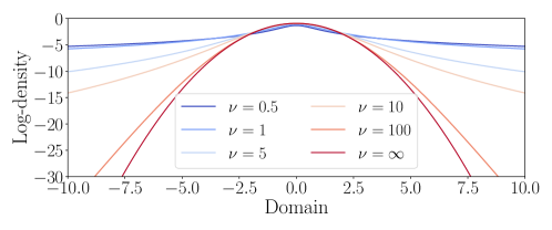
Figure 1: Logarithm of the probability density of the univariate standard Student’s $t$ distribution $\mathcal{T}_{\nu}\left(0,1\right)$ for different values of the degrees of freedom parameter $\nu$. As $\nu=\infty$, Student’s $t$ $\mathcal{T}_{\infty}\left(0,1\right)$ is equivalent to the univariate standard Gaussian distribution $\mathcal{N}(0,1)$.

Sampling from posterior distributions in high dimensions under the Student’s $t$ MRF prior is cumbersome. To improve the efficiency of the prior implementation one can utilize the GSM representation of the Student’s $t$ distribution. In this case, the mixing distribution is inverse-gamma [8]. By incorporating this property, we can transform the original prior model into a hierarchical one, where the target difference random vector follows (conditionally) a more tractable Gaussian distribution. Therefore, we can write the GSM prior density for the $i$-th component of difference random vector as follows

$$p({u}_{i})=\int_{0}^{\infty}p({u}_{i}\;|\;\tau^{2},{w}_{i}^{2})p({w}_{i}^{2})\,\mathrm{d}{w}_{i}^{2},$$ (10a)

$$({u}_{i}\;|\;\tau^{2},{w}_{i}^{2})\sim\mathcal{N}\left({\mu},\tau^{2}w_{i}^{2}\right),\quad{w}_{i}^{2}\sim\text{IG}\left(\nicefrac{{\nu}}{{2}},\nicefrac{{\nu}}{{2}}\right),$$ (10b)

where ${w}_{i}^{2}$ is the mixing random variable and $\text{IG}(a,b)$ denotes the inverse-gamma distribution with shape and scale parameters $a,b$, such that the density is defined as

$$p(w_{i}^{2})=\frac{b^{a}}{\Gamma(a)}(w_{i}^{2})^{-a-1}\exp\left(-\frac{b}{w_{i}^{2}}\right).$$ (11)

Note that each mixing variable $w_{i}^{2}$ appears to control the variance locally for each difference component $u_{i}$. Analogously, the scale-squared parameter $\tau^{2}$ controls the prior variance globally across the domain. As this parameter becomes important for the prior specification, we assume it is uncertain and endow it with another inverse-gamma hyperprior. In this case, we set the shape parameter as $a=1$ and the scale parameter as $b=10^{-4}$ (see, e.g., [41]).

By utilizing GSM in eq. 10b and the linear relation described in eq. 5, we can establish a conditionally Gaussian MRF prior for the random vector $\bm{X}$. In Gaussian MRFs, the precision matrix plays a crucial role, as its sparsity structure determines the neighborhood system that explains conditional relationships among the elements of $\bm{X}$. In edge-preserving inverse problems, the precision matrix is constructed based on the differences between the elements of the parameter vector. Specifically, it depends on the matrix $\bm{L}$ (for detailed information, refer to [7, p.68]). Consequently, we can express the prior precision matrix as

$$\bm{\Lambda}(\tau^{2},\bm{w}^{2})=\bm{L}^{\mathsf{T}}\bm{W}(\tau^{2},\bm{w}^{2})\bm{L},\qquad\bm{W}(\tau^{2},\bm{w}^{2}):=\operatorname{diag}\left(\frac{1}{\tau^{2}w_{1}^{2}},\ldots,\frac{1}{\tau^{2}w_{d}^{2}}\right).$$ (12)

As a result, by using the GSM of the $t$ distribution on the random vector of differences $\bm{U}$, we establish a hierarchical prior for $\bm{X}$ as follows

$$p(\bm{x},\tau^{2},\bm{w}^{2})=p(\bm{x}\;|\;\tau^{2},\bm{w}^{2})p(\bm{w}^{2}\;|\;\nu)p(\nu)p(\tau^{2}),$$ (13a)

$$(\bm{x}\;|\;\tau^{2},\bm{w}^{2})\sim\mathcal{N}\left(\bm{\mu},\bm{\Lambda}^{-1}(\tau^{2},\bm{w}^{2})\right),$$ (13b)

$$\tau^{2}\sim\text{IG}\left(a,b\right),\quad\bm{w}^{2}\;|\;\nu\sim\prod_{i=1}^{d}\text{IG}\left(\nicefrac{{\nu}}{{2}},\nicefrac{{\nu}}{{2}}\right),\quad\nu\sim p(\nu),$$ (13c)

where the squaring $\bm{w}^{2}$ applies element-wise, and $p(\nu)$ denotes the prior on the degrees of freedom parameter $\nu$, which is discussed next.

Remark 3.1.

The global-local scheme associated with the hierarchical prior eq. 13a shares similarities with the horseshoe prior [25], however, the hyperpriors for the local and global scale parameters are defined as half-Cauchy distributions for which the GSM representation has a different form. Moreover, the hierarchical prior eq. 13a is also related to the models discussed in [42, 43], which employ a generalized inverse-gamma distribution as hyperprior.

3.2 Modeling the degrees of freedom

The estimation of the degrees of freedom parameter $\nu$ of the Student’s $t$ distribution has been actively studied [12, 13, 14]. The choice of the prior distribution is known to be challenging as this parameter is typically poorly identified from the data [44].

We consider two popular prior choices [15, 18]:

1. $\text{Ga}(\nu;\,a=2,b=0.1,\mu=0)$, the gamma distribution with the shape parameter $a\in\mathbb{R}_{>0}$, rate parameter $b\in\mathbb{R}_{>0}$ and location parameter $\mu\in\mathbb{R}_{>0}$. The gamma probability density is defined as

   $$p(\nu)=\frac{b^{a}}{\Gamma(a)}(\nu-\mu)^{a-1}\exp\left[-b(\nu-\mu)\right],\qquad\nu\geq\mu.$$ (14)

2. $\log\mathcal{N}\left(\nu;\,\mu=1,\sigma=1\right)$, the log-normal distribution with parameters $\mu\in\mathbb{R}$ and $\sigma^{2}\in\mathbb{R}_{>0}$. The log-normal probability density is defined as

   $$p(\nu)=\frac{1}{\nu\sqrt{2\pi\sigma^{2}}}\exp\left(-\frac{(\log\nu-\mu)^{2}}{2\sigma^{2}}\right).$$ (15)

In computational statistics, it is recommended to set a lower limit $\nu>1$ on the gamma distribution. This ensures the first moment (mean) of the $t$ distribution exists. Therefore, in addition to the previous prior choices, we compare the following thresholded gamma distributions:

1. $\text{Ga}(\nu;\,a=2,b=0.1,\mu=1)$, a thresholded Gamma distribution which is equivalent to the prior choice $1$, but now excluding values $\nu\leq 1$. We remark that in this case $\mu\neq 0$, and we further employ notation $\mathrm{Ga}_{\nu>\mu}(\nu;\,a,b)$ to emphasise the application of a threshold.

2. $\text{Ga}(\nu;\,a=3,b=0.1,\mu=1)$, a thresholded Gamma distribution with shape $a=3$. This distribution has mode at $20$ and puts more probability mass away from the interval $(1,10)$ as compared to the first three prior options. Thus, it promotes larger values of $\nu$ resulting in the smooth behavior rather than piecewise constant. This can be beneficial, if the task is to reconstruct smooth features in the object rather than sharp edges.

We illustrate the performance of the four chosen priors in Section 5.1.

3.3 Posterior under the Student’s $t$ prior

The Bayesian inverse problem of estimating the posterior eq. 6b under the hierarchical prior in eq. 13a is written as the hierarchical Bayesian inverse problem of determining the posterior density

$$p(\bm{x},\sigma_{\mathrm{obs}}^{2},\tau^{2},\bm{w}^{2},\nu\;|\;\bm{y})=p(\bm{y}\;|\;\bm{x},\sigma_{\mathrm{obs}}^{2})p(\sigma_{\mathrm{obs}}^{2})\,p(\bm{x}\;|\;\tau^{2},\bm{w}^{2})p(\tau^{2})p(\bm{w}^{2}\;|\;\nu)p(\nu).$$ (16)

In particular, the full conditional densities for each parameter are

$$p\left(\bm{x}\;|\;\sigma_{\mathrm{obs}}^{2},\tau^{2},\bm{w}^{2}\right) \propto p(\bm{y}\;|\;\bm{x},\sigma_{\mathrm{obs}}^{2})p(\bm{x}\;|\;\tau^{2},\bm{w}^{2}),$$ (17a)

$$p(\sigma_{\mathrm{obs}}^{2}\;|\;\bm{x}) \propto p(\bm{y}\;|\;\bm{x},\sigma_{\mathrm{obs}}^{2})p(\sigma_{\mathrm{obs}}^{2}),$$ (17b)

$$p(\tau^{2}\;|\;\bm{x},\bm{w}^{2}) \propto p(\bm{x}\;|\;\tau^{2},\bm{w}^{2})p({\tau}^{2}),$$ (17c)

$$p(\bm{w}^{2}\;|\;\bm{x},\tau^{2},\nu) \propto p(\bm{x}\;|\;\tau^{2},\bm{w}^{2})p(\bm{w}^{2}\;|\;\nu),$$ (17d)

$$p(\nu\;|\;\bm{w}^{2}) \propto p(\bm{w}^{2}\;|\;\nu)p(\nu).$$ (17e)

Now we can replace the corresponding densities on each conditional to derive them in closed form when possible.

Conditional 1. The density on $\bm{x}\;|\;\sigma_{\mathrm{obs}}^{2},\tau^{2},\bm{w}^{2}$ sets a linear Gaussian Bayesian inverse problem which has closed form solution for the posterior (see, e.g., [6, p.78]). Therefore

$$p\left(\bm{x}\;|\;\sigma_{\mathrm{obs}}^{2},\tau^{2},\bm{w}^{2}\right) \propto\exp\left(-\frac{1}{2}\left(\frac{1}{\sigma_{\mathrm{obs}}^{2}}\left\|\bm{y}-\bm{A}\bm{x}\right\|_{2}^{2}+\bigl{\|}\bm{\Lambda}^{\nicefrac{{1}}{{2}}}(\tau^{2},\bm{w}^{2})\,\bm{x}\bigr{\|}_{2}^{2}\right)\right)$$ (18a)

$$\bm{x}\;|\;\sigma_{\mathrm{obs}}^{2},\tau^{2},\bm{w}^{2} \sim\mathcal{N}\left(\widetilde{\bm{\mu}}(\tau^{2},\bm{w}^{2})\,,\,\widetilde{\bm{\Lambda}}^{-1}(\tau^{2},\bm{w}^{2})\right),$$ (18b)

with the precision and mean parameters

$$\widetilde{\bm{\Lambda}}(\tau^{2},\bm{w}^{2})=\frac{1}{\sigma_{\mathrm{obs}}^{2}}\bm{A}^{\mathsf{T}}\bm{A}+\bm{\Lambda}(\tau^{2},\bm{w}^{2}),\qquad\widetilde{\bm{\mu}}=\widetilde{\bm{\Lambda}}^{-1}(\tau^{2},\bm{w}^{2})\left(\frac{1}{\sigma_{\mathrm{obs}}^{2}}\bm{A}^{\mathsf{T}}\bm{y}\right);$$ (19)

recall the prior precision matrix $\bm{\Lambda}(\tau^{2},\bm{w}^{2})$ is defined in eq. 12. The Cholesky factorization provides the most direct sampling algorithm for a Gaussian distribution. In this approach, a sample is obtained as $\bm{x}^{\star}=\widetilde{\bm{\mu}}+\widetilde{\bm{\Lambda}}^{-\nicefrac{{1}}{{2}}}\bm{u}$, where $\bm{u}\sim\mathcal{N}(\bm{0},\bm{I}_{d})$ represents a standard Gaussian random vector, and $\widetilde{\bm{\Lambda}}^{\nicefrac{{1}}{{2}}}$ denotes a lower triangular matrix with positive real diagonal entries. However, the Cholesky strategy becomes computationally prohibitive due to the need for factorizing the matrix $\widetilde{\bm{\Lambda}}(\tau^{2},\bm{w}^{2})$. This difficulty also arises in MCMC algorithms for Gaussian distributions, such as preconditioned Crank–Nicolson [45]. To overcome this, we can use Krylov subspace methods to sample from the Gaussian conditional distribution in eq. 18. In particular, we can draw a sample from $p\left(\bm{x}\;|\;\sigma_{\mathrm{obs}}^{2},\tau^{2},\bm{w}^{2}\right)$ through randomized optimization. For further details on this formulation, refer to [7, p.81].

Conditional 2. The conditional density for the noise variance $\sigma_{\mathrm{obs}}^{2}$ is obtained as the product of Gaussian and inverse-gamma densities. Through conjugate relations, this results is another inverse-gamma density that can be directly simulated

$$p(\sigma_{\mathrm{obs}}^{2}\;|\;\bm{x}) \propto p(\bm{y}\;|\;\bm{x},\sigma_{\mathrm{obs}}^{2})p(\sigma_{\mathrm{obs}}^{2})$$ (20a)

$$\propto(\sigma_{\mathrm{obs}}^{2})^{-\nicefrac{{m}}{{2}}}\exp\left(-\frac{1}{2\sigma_{\mathrm{obs}}^{2}}\left\|\bm{y}-\bm{A}\bm{x}\right\|_{2}^{2}\right)\left[(\sigma_{\mathrm{obs}}^{2})^{-a-1}\exp\left(-\frac{b}{\sigma_{\mathrm{obs}}^{2}}\right)\right]$$ (20b)

$$\propto(\sigma_{\mathrm{obs}}^{2})^{-(\nicefrac{{m}}{{2}}+a)-1}\exp\left(-\left[\frac{1}{2}\left\|\bm{y}-\bm{A}\bm{x}\right\|_{2}^{2}+b\right]\frac{1}{\sigma_{\mathrm{obs}}^{2}}\right)$$ (20c)

$$\sigma_{\mathrm{obs}}^{2}\;|\;\bm{x} \sim\text{IG}\left(\frac{m}{2}+a,\frac{1}{2}\left\|\bm{y}-\bm{A}\bm{x}\right\|_{2}^{2}+b\right),$$ (20d)

recall the hyperprior shape and scale parameters can be fixed as $a=1$ and $b=10^{-4}$, respectively.

Conditional 3. The conditional density for the squared-scale parameter $\tau^{2}$ is another inverse-gamma density

$$p(\tau^{2}\;|\;\bm{x},\bm{w}^{2}) \propto p(\bm{x}\;|\;\tau^{2},\bm{w}^{2})p({\tau}^{2})$$ (21a)

$$\propto(\tau^{2})^{-\nicefrac{{k}}{{2}}}\exp\left(-\sum_{i=1}^{k}\frac{([\bm{L}\bm{x}]_{i}-\mu)^{2}}{2\tau^{2}w_{i}^{2}}\right)\left[(\tau^{2})^{-a-1}\exp\left(-\frac{b}{\tau^{2}}\right)\right]$$ (21b)

$$\propto(\tau^{2})^{-(\nicefrac{{k}}{{2}}+a)-1}\exp\left(-\left[\sum_{i=1}^{k}\frac{([\bm{L}\bm{x}]_{i}-\mu)^{2}}{2w_{i}^{2}}+b\right]\frac{1}{\tau^{2}}\right)$$ (21c)

$$\tau^{2}\;|\;\bm{x},\bm{w}^{2} \sim\text{IG}\left(\frac{k}{2}+a,\sum_{i=1}^{d}\frac{([\bm{L}\bm{x}]_{i}-\mu)^{2}}{2w_{i}^{2}}+b\right),$$ (21d)

where $k=\{d,2d\}$ in one- and two-dimensional problems, respectively. Recall the hyperprior shape and scale parameters are the same as those of the noise variance.

Conditional 4. Since the auxiliary parameters are independent, we can derive the conditional density for each component of $\bm{w}^{2}$ as follows

$$p(w_{i}^{2}\;|\;\bm{x},\tau^{2},\nu) \propto p(\bm{x}\;|\;\tau^{2},\bm{w}^{2})p(\bm{w}^{2}\;|\;\nu)$$ (22a)

$$\propto(w_{i}^{2})^{-\nicefrac{{1}}{{2}}}\exp\left(-\frac{([\bm{L}\bm{x}]_{i}-\mu)^{2}}{2\tau^{2}w_{i}^{2}}\right)\left[(w_{i}^{2})^{-\nicefrac{{\nu}}{{2}}-1}\exp\left(-\frac{\nu}{2w_{i}^{2}}\right)\right]$$ (22b)

$$\propto(w_{i}^{2})^{-(\nicefrac{{1}}{{2}}+\nicefrac{{\nu}}{{2}})-1}\exp\left(-\left[\frac{([\bm{L}\bm{x}]_{i}-\mu)^{2}}{2\tau^{2}}+\frac{\nu}{2}\right]\frac{1}{w_{i}^{2}}\right)$$ (22c)

$$w_{i}^{2}\;|\;\bm{x},\tau^{2},\nu \sim\text{IG}\left(\frac{\nu+1}{2},\,\frac{([\bm{L}\bm{x}]_{i}-\mu)^{2}}{2\tau^{2}}+\frac{\nu}{2}\right).$$ (22d)

Conditional 5. Finally, the conditional density for the degrees of freedom $\nu$ is written as

$$p(\nu\;|\;\bm{w}^{2})\propto p(\nu)p(\bm{w}^{2}\;|\;\nu)=p(\nu)\prod_{i=1}^{d}\frac{(\nicefrac{{\nu}}{{2}})^{\nicefrac{{\nu}}{{2}}}}{\Gamma(\nicefrac{{\nu}}{{2}})}({w}_{i}^{2})^{-\nicefrac{{\nu}}{{2}}-1}\exp\left(-\frac{\nu}{2{w}_{i}^{2}}\right).$$ (23)

This one-dimensional density can be sampled within the Gibbs iterations using classical algorithms such as rejection sampling or random walk Metropolis (RWM). In our study, after comparing both methods, we choose to use RWM. For this RWM-within-Gibbs sampling step we can also perform a few extra within-Gibbs iterations (i.e., a within-Gibbs burn-in $\bar{n}_{b}$ and thinning $\bar{n}_{t}$) in order to accelerate the convergence of the Gibbs chain and to reduce correlation in the resulting posterior samples (see, e.g., [46, p.213]). To improve the convergence, we use vanishing adaptation during the within-Gibbs burn-in [47]. This type of adaptation ensures that the proposal depends on recent sates in the chain less and less strongly, i.e., the adaptation gradually disappears from the proposal.

4 Computation procedure for posterior sampling

We describe two MCMC algorithms to sample from the posterior distribution under the Student’s $t$ prior. The first algorithm, the Gibbs sampler, exploits the GSM representation of the Student’s $t$ distribution. The other algorithm, NUTS, uses the traditional Student’s $t$ formulation; we consider NUTS to validate the numerical results obtained using Gibbs sampling.

We remark that, from a practical perspective, in MCMC we generate $n_{s}$ states of the chain that are only selected after discarding $n_{b}$ samples during the warm up phase of the algorithm (burn-in period), and the sample chain values are only stored every $n_{t}$ iterations since for large enough $n_{t}$ the samples are virtually independent (lagging steps). As a result, we need to draw $n=n_{b}+n_{s}n_{t}$ Markov chain steps to obtain $n_{s}$ quasi-independent samples from the posterior. Furthermore, the quality of a chain produced by a sampler can be quantitatively measured using the effective sample size (ESS). This metric reflects the amount of uncertainty within the chain due to autocorrelation. Therefore, if $\rho^{(i)}$ denotes the autocorrelation at the $i$-th lag, the ESS can be calculated as follows

$$n_{\mathrm{eff}}=\frac{n_{s}}{1+2\sum_{i=1}^{n_{s}}(\nicefrac{{\rho^{(i)}}}{{\rho^{(0)}}})}\approx\left\lceil\frac{n_{s}}{\tau_{\mathrm{int}}}\right\rceil,$$ (24)

where $\tau_{\mathrm{int}}$ stands for the integrated autocorrelation time (IACT). The definition of the ESS intuitively means that the larger chain autocorrelation is, the smaller effective sample size is. Hence, while sampling one should target values of $n_{\text{eff}}$ as close as possible to the sample size $n_{s}$.

4.1 Gibbs sampler

Gibbs sampling operates as an iterative algorithm that systematically selects a single variable from a model and resamples it based on its conditional distribution, given the other variables. The sampling process is based on the fact that, under mild conditions, the set of full conditional distributions determines the joint distribution [48]. Moreover, convergence conditions of the Gibbs sampler are discussed in [49, 50]. By deriving the full conditional densities of all parameters, as shown in Section 3.3, we can use the Gibbs sampler to generate a Markov chain with stationary distribution equivalent to the posterior distribution eq. 16.

In Gibbs sampling, the process of choosing which parameter to sample (i.e., the variable index), often referred to as the scan order, plays a crucial role [51]. Two predominant scan orders are employed: random scan and systematic scan. In random scan, variables are chosen uniformly and independently at random during each iteration. In systematic scan, a predetermined permutation is chosen, with variables consistently selected in that specified order throughout the sampling process. Without loss of generality we follow a random scan strategy; this is mainly due to the fact that this Gibbs sampler version is reversible with respect to the posterior. The resulting Gibbs sampler applied to posterior eq. 16 is summarized (with a slight abuse of notation) in Algorithm 1.

Data: Gibbs parameters: number of samples $n_{s}$, burn-in $n_{b}$, thinning $n_{t}$. RWM-within-Gibbs parameters: warm-up $\bar{n}_{b}$ and thinning $\bar{n}_{t}$.                               Posterior conditional densities eq. 17.

1 Initialize $\bm{x}$, $\sigma_{\mathrm{obs}}^{2}$, $\tau^{2}$, $\bm{w}^{2}$, $\nu$

2 $n\leftarrow n_{s}n_{t}+n_{b}$

3 $j\leftarrow 1$

4 for $i\leftarrow 1$ to $n$ do

5       $k\leftarrow\texttt{randint}([1,5])$

6        # generate the variable index

7       switch $k$ do

8             case $1$ do

9                   compute posterior mean $\widetilde{\bm{\mu}}(\tau^{2},\bm{w}^{2})$ and precision matrix $\widetilde{\bm{\Lambda}}\;(\tau^{2},\bm{w}^{2})$

10                  sample $\bm{x}\sim\mathcal{N}(\widetilde{\bm{\mu}},\widetilde{\bm{\Lambda}}^{-1})$

11                  

12             case $2$ do sample $\sigma_{\mathrm{obs}}^{2}\sim p(\cdot\;|\;\bm{x})$ in closed form according to eq. 20d

13              case $3$ do sample $\tau^{2}\sim p(\cdot\;|\;\bm{x},\bm{w}^{2})$ in closed form according to eq. 21d

14              case $4$ do sample $\bm{w}^{2}\sim p(\cdot\;|\;\bm{x},\tau^{2},\nu)$ in closed form according to eq. 22d

15              case $5$ do sample $\nu\sim p(\cdot\;|\;\bm{w}^{2})$ in eq. 23 using RWM with warm-up $\bar{n}_{b}$ and thinning $\bar{n}_{t}$

16             

17       end switch

18      if $i>n_{b}$ and $\mathrm{mod}(i,n_{t})=0$ then

19             $\bm{x}^{(j)}\leftarrow\bm{x}$, $(\sigma_{\mathrm{obs}}^{2})^{(j)}\leftarrow\sigma_{\mathrm{obs}}^{2}$, $(\tau^{2})^{(j)}\leftarrow\tau^{2}$, $(\bm{w}^{2})^{(j)}\leftarrow\bm{w}^{2}$, $\nu^{(j)}\leftarrow\nu$

20            $j\leftarrow j+1$

21            

22       end if

23      

24 end for

return $\{\bm{x}^{(j)}\}_{j=1}^{n_{s}}$, $\{(\sigma_{\mathrm{obs}}^{2})^{(j)}\}_{j=1}^{n_{s}}$, $\{(\tau^{2})^{(j)}\}_{j=1}^{n_{s}}$, $\{(\bm{w}^{2})^{(j)}\}_{j=1}^{n_{s}}$, $\{\nu^{(j)}\}_{j=1}^{n_{s}}$

Algorithm 1 Random scan Gibbs sampler

4.2 NUTS sampler

We introduced the Bayesian inverse problem of estimating the posterior eq. 16 under the MRF prior based on the GSM representation of the Student’s $t$ distribution. The GSM formulation lends itself well to the application of the Gibbs sampler, due to the availability of conditional densities for each parameter.

Alternatively, we consider imposing Student’s $t$ distribution on the vector of increments $\bm{u}=\bm{L}\bm{x}$ without the GSM representation. In this case, the posterior eq. 6b can be modelled hierarchically as follows

$$p(\bm{x},\tau^{2},\nu\;|\;\bm{y})=p(\bm{y}\;|\;\bm{x})\,p(\bm{L}\bm{x}\;|\;\tau^{2},\nu)p(\tau^{2})p(\nu),$$ (25a)

$$(\bm{L}\bm{x}\;|\;\tau^{2},\nu)\sim\mathcal{T}_{\nu}\left(\mu,\tau^{2}\right),$$ (25b)

$$\tau^{2}\sim\text{IG}(a,b),\quad\nu\sim p(\nu).$$ (25c)

To sample from the posterior eq. 25a, we employ NUTS [31]. This method requires the logarithm of posterior and also its gradient. The logarithm of posterior eq. 25a is defined as follows

$$\log p(\bm{x},\tau^{2},\nu\;|\;\bm{y})=\log p(\bm{y}\;|\;\bm{x})+\log p(\bm{L}\bm{x}\;|\;\tau^{2},\nu)+\log p(\tau^{2})+\log p(\nu).$$ (26)

Since our formulation relies on linear forward models and the likelihood is Gaussian, the log-likelihood and its derivative with respect to the target parameter $\bm{x}$ are well-known (see, e.g., [52, p.11]). However, as the prior distribution is more involved, we now write its natural logarithm and associated derivatives. The log-prior on $\bm{x}$ is

$$\begin{split}\log p(\bm{L}\bm{x}\;|\;\tau^{2},\nu)\propto&\,d\left[\log\Gamma\left(\frac{\nu+1}{2}\right)-\log\Gamma\left(\frac{\nu}{2}\right)-\frac{1}{2}\log(\pi\nu)-\frac{1}{2}\log(\tau^{2})\right]-\\ &\left(\frac{\nu+1}{2}\right)\sum_{i=1}^{d}\log\left(1+\frac{([\bm{L}\bm{x}]_{i}-\mu)^{2}}{\nu\tau^{2}}\right),\end{split}$$ (27)

and its partial derivatives with respect to the parameters $\bm{x}$, $\tau^{2}$ and $\nu$ are

$$\frac{\partial}{\partial\bm{x}}\log p(\bm{L}\bm{x}\;|\;\tau^{2},\nu)\propto \,-\left(\frac{\nu+1}{1+\frac{(\bm{L}\bm{x}-\mu)^{2}}{\nu\tau^{2}}}\right)\left(\frac{\bm{L}\bm{x}-\mu}{\nu\tau^{2}}\right)\bm{L},$$ (28a)

$$\frac{\partial}{\partial\tau^{2}}\log p(\bm{L}\bm{x}\;|\;\tau^{2},\nu)\propto \,-\frac{d}{2\tau^{2}}+\sum_{i=1}^{d}\left[\left(\frac{\nu+1}{2}\right)\left(\frac{1}{1+\frac{(\bm{L}\bm{x}-\mu)^{2}}{\nu\tau^{2}}}\right)\left(\frac{([\bm{L}\bm{x}]_{i}-\mu)^{2}}{(\nu(\tau^{2}))^{2}}\right)\right],$$ (28b)

$$\frac{\partial}{\partial\nu}\log p(\bm{L}\bm{x}\;|\;\tau^{2},\nu)\propto \,\frac{d}{2}\Psi\left(\frac{\nu+1}{2}\right)-\frac{d}{2}\Psi\left(\frac{\nu}{2}\right)-\frac{d}{2\nu}-\frac{1}{2}\sum_{i=1}^{d}\log\left(1+\frac{([\bm{L}\bm{x}]_{i}-\mu)^{2}}{\nu\tau^{2}}\right)+$$

$$\frac{\nu+1}{2}\sum_{i=1}^{d}\left(\frac{1}{1+\frac{(\bm{L}\bm{x}-\mu)^{2}}{\nu\tau^{2}}}\right)\left(\frac{([\bm{L}\bm{x}]_{i}-\mu)^{2}}{\nu^{2}\tau^{2}}\right),$$ (28c)

where $\Psi(\cdot)$ denotes the digamma function, or the logarithmic derivative of the gamma function $\Gamma$.

We now follow the same procedure for the hyperparameters, assuming a gamma prior $\text{Ga}(\nu;\,a,b)$ on the degrees of freedom parameter. The logarithms and derivatives of the hyperprior for $\tau^{2}$ and prior for $\nu$ are defined as

$$\log p(\tau^{2}) \propto(-a-1)\log(\tau^{2})-\frac{b}{\tau^{2}},\quad \frac{\partial}{\partial\tau^{2}}\log p(\tau^{2}) \propto-\frac{a+1}{\tau^{2}}+\frac{b}{(\tau^{2})^{2}},$$ (29a)

$$\log p(\nu) \propto(a-1)\log(\nu)-b\,\nu,\quad \frac{\partial}{\partial\nu}\log p(\nu) \propto\frac{a-1}{\nu}-b.$$ (29b)

5 Numerical experiments

In the following, we illustrate the use of the proposed Student’s $t$ priors for Bayesian inversion. We consider linear inverse problems arising in signal processing and imaging science. The first example is one-dimensional deconvolution problem that allows us to test multiple parameter settings in our computational framework. The second example is the image deblurring problem.

In our test problems, the point estimates $\bar{\bm{x}}$ (posterior mean) of the target parameter are evaluated using the relative reconstruction error defined as

$$\text{relerr}:=\frac{\left\|\bar{\bm{x}}-\bm{x}^{\mathrm{true}}\right\|_{2}}{\left\|\bm{x}^{\mathrm{true}}\right\|_{2}},$$ (30)

where $\bm{x}^{\mathrm{true}}$ denotes the underlying true solution.

5.1 One-dimensional deconvolution

We consider the inverse problem of identifying a signal $x:[0,1]\rightarrow\mathbb{R}$ from noisy convolved data. The mathematical model for convolution can be written as a Fredholm integral equation of the first kind

$$y(t)=\int_{0}^{1}\mathcal{A}(t,s)x(s)ds\quad\text{with}\quad\mathcal{A}(t,s)=\exp\left(-\frac{1}{2\sigma^{2}}(t-s)^{2}\right),\qquad 0\leq t\leq 1,$$ (31)

where $y(t)$ denotes the convolved signal and we employ a Gaussian convolution kernel $\mathcal{A}(t)$ with a fixed parameter $\sigma$ which controls the width of the blurring kernel.

A finite-dimensional representation of eq. 31 is employed in practice. After discretizing the signal domain using $d=128$ points, the convolution model can be expressed as a system of linear algebraic equations $\bm{y}=\bm{A}\bm{x}$. We consider synthetic observation data $\bm{y}$ with $m=d-2$ equally-spaced elements (excluding two boundary points).

We compare two different signals, a piecewise constant (or sharp) signal and smooth signal, to illustrate the flexibility of the proposed priors and their performance in recovering discontinuous signals as well as smooth. Figure 2 shows the two underlying true signals together with the noisy observational data. The data were obtained according to model eq. 31 with parameter $\sigma=4$ for the piecewise constant signal and $\sigma=8$ for smooth. The data were corrupted by adding Gaussian noise with standard deviation $\sigma_{\mathrm{obs}}^{\mathrm{true}}=8.654\times 10^{-3}$ for the piecewise constant signal and $\sigma_{\mathrm{obs}}^{\mathrm{true}}=4.368\times 10^{-2}$ for the smooth signal.

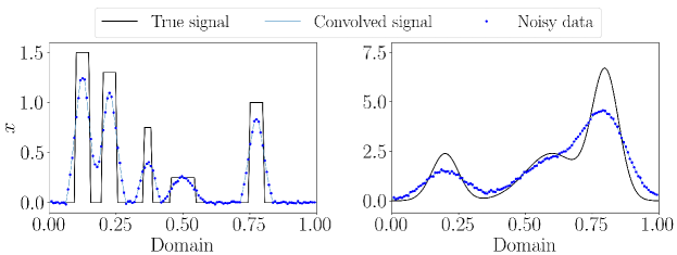
Figure 2: One-dimensional deconvolution example. Left: sharp signal; right: smooth signal. Noisy convolved data (dots).

Firstly, we perform a prior study for the degrees of freedom parameter $\nu$ to select the best suitable option for our setting. Next, for the selected prior, we compare Gibbs and NUTS samplers and their efficiency in exploring the posterior distribution. Finally, we compare solutions obtained with the Student’s $t$ prior against the results obtained using another popular prior — the Laplace prior.

Prior comparison. We study four different options for the prior distribution to model the degrees of freedom $\nu$ as described in Section 3.2. We compare two distribution options discussed in [18]: gamma distribution $\text{Ga}(\nu;\,2,0.1)$ and log-normal distribution $\log\mathcal{N}\left(\nu;\,1,1\right)$ with two thresholded variations of Gamma distribution: $\text{Ga}_{\nu>1}(\nu;\,2,0.1)$ and $\text{Ga}_{\nu>1}(\nu;\,3,0.1)$.

We explore the resulting posterior distribution using the Gibbs sampler with the number of samples $n_{s}=2\times 10^{4}$, the global burn-in (or warm-up) period $n_{b}=2\times 10^{3}$, and lag (or thinning number) $n_{t}=20$. To sample the degrees of freedom parameter $\nu$ within Gibbs, we use RWM sampler that produces $1$ sample with burn-in period $\bar{n}_{b}=100$ and thinning $\bar{n}_{b}=10$. We choose values for $\bar{n}_{b}$ and $\bar{n}_{t}$ based on numerical studies. Since conditional of $\nu$ eq. 23 is computationally inexpensive to evaluate we can afford to perform extra within-Gibbs iterations (burn-in and thinning) to improve the resulting sub-chain of $\nu$.

Posterior statistics for the target parameter $\bm{x}$ and the local scale parameter $\bm{w}$ for both piecewise constant and smooth signals are shown in Figures 3 and 4, respectively. The piecewise constant signal is approximated with a smaller relative error when the first two priors, $\text{Ga}(\nu;\,2,0.1)$ and $\log\mathcal{N}\left(\nu;\,1,1\right)$, are used since they allow for values $\nu<1$ (which corresponds to more heavy-tailed behaviour than Cauchy) as compared to the thresholded versions of Gamma distribution, $\text{Ga}_{\nu>1}(\nu;\,2,0.1)$ and $\text{Ga}_{\nu>1}(\nu;\,3,0.1)$, that restrict parameter $\nu$. In the smooth signal scenario, the first two priors result in worse signal reconstructions: note poor approximation of the peak located at $0.8$. A possible explanation behind such artefacts in the solution is that we impose prior on the difference vector and, therefore, penalize changes in curvature of the smooth signal. For the more suitable prior choices (priors $\text{Ga}_{\nu>1}(\nu;\,2,0.1)$ and $\text{Ga}_{\nu>1}(\nu;\,3,0.1)$), less artifacts are present in the smooth signal approximation and the reconstruction errors are smaller.

In Figure 5, we show probability density functions of prior distributions and corresponding histograms of posterior distributions for both signals. The first three prior distributions ($\text{Ga}(\nu;\,2,0.1)$, $\log\mathcal{N}\left(\nu;\,1,1\right)$, and $\text{Ga}_{\nu>1}(\nu;\,2,0.1)$) have more probability mass placed on the interval $(1,10)$ and, therefore, promote small values for the degrees of freedom parameter corresponding to the edge-promoting rather than smoothing behaviour. On the other hand, distribution $\text{Ga}_{\nu>1}(\nu;\,3,0.1)$ has mode at $20$ and assumes more mass far away from $1$. However, when prior $\text{Ga}_{\nu>1}(\nu;\,3,0.1)$ is used, we see that the posterior distribution for the smooth signal coincides with the prior distribution meaning that this prior is too strong and we do not explore posterior of $\nu$ at all. In general, the posterior histograms illustrate the flexibility of the prior to model different structural features. The model finds values of $\nu$ that better represent the data: in the piecewise constant case, it tends to favour small values of the degrees of freedom parameter, while in the smooth case, it tends to favour larger values.

In Table 1, we report posterior statistics (sample mean, standard deviation and effective sample size) for the scalar parameters: degrees of freedom $\nu$, global scale parameter $\tau$ and the noise standard deviation $\sigma_{\mathrm{obs}}$.

Based on the analysis, we choose $\text{Ga}_{\nu>1}(\nu;\,2,0.1)$ as a prior distribution for the degrees of freedom parameter. This choice results in good reconstructions for both discontinuous and smooth cases and, in addition, allows avoiding possible pathological behavior via restricting values of $\nu$. We remark that the values of the proposal scaling in the RWM-within-Gibbs after adaptation are around $0.555$ and $1.067$, for the sharp and smooth signals, respectively.

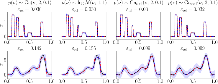
Figure 3: Comparison of posterior statistics for target parameter $\bm{x}$ using four different priors on the degrees of freedom $\nu$. Columns from left to right: 1) gamma prior with shape $2$ and rate $0.1$; 2) log-normal prior with scale and variance $1$; 3) thresholded gamma prior with shape $2$ and rate $0.1$; and 4) thresholded gamma prior with shape $3$ and rate $0.1$. Top row: sharp signal, bottom row: smooth signal. True solution (black solid line), posterior median (red dashed line), posterior mean (blue dotted line), and $95\%$ highest density interval (shaded area).

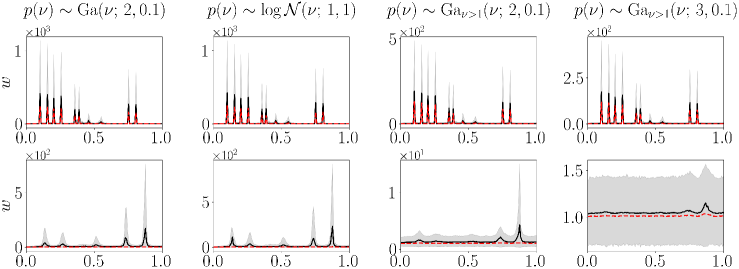
Figure 4: Comparison of posterior statistics for the local scale parameter $\bm{w}$ using four different priors on the degrees of freedom $\nu$. Columns from left to right: 1) gamma prior with shape $2$ and rate $0.1$; 2) log-normal prior with scale and variance $1$; 3) thresholded gamma prior with shape $2$ and rate $0.1$; and 4) thresholded gamma prior with shape $3$ and rate $0.1$. Top row: sharp signal, bottom row: smooth signal. Posterior median (red dashed line) and mean (black solid line), and $95\%$ highest density interval (shaded area).

Signal	Prior for $\nu$	Parameter	Mean	Std	$n_{\mathrm{eff}}$
		$\nu$	$0.736$	$0.107$	$3\,954$
	$\text{Ga}(\nu;\,2,0.1)$	$\tau$	$6.269\times 10^{-3}$	$1.906\times 10^{-3}$	$1\,122$
		$\sigma_{\mathrm{obs}}$	$8.397\times 10^{-3}$	$6.108\times 10^{-4}$	$12\,447$
		$\nu$	$0.726$	$0.105$	$4\,411$
	$\log\mathcal{N}(\nu;\,1,1)$	$\tau$	$6.179\times 10^{-3}$	$1.814\times 10^{-3}$	$1\,298$
Sharp		$\sigma_{\mathrm{obs}}$	$8.401\times 10^{-3}$	$6.121\times 10^{-4}$	$14\,046$
signal		$\nu$	$1.112$	$0.079$	$4\,846$
	$\text{Ga}_{\nu>1}(\nu;\,2,0.1)$	$\tau$	$10.493\times 10^{-3}$	$3.989\times 10^{-3}$	$684$
		$\sigma_{\mathrm{obs}}$	$8.393\times 10^{-3}$	$6.185\times 10^{-4}$	$12\,683$
		$\nu$	$1.165$	$0.095$	$3\,338$
	$\text{Ga}_{\nu>1}(\nu;\,3,0.1)$	$\tau$	$11.214\times 10^{-3}$	$4.215\times 10^{-3}$	$622$
		$\sigma_{\mathrm{obs}}$	$8.395\times 10^{-3}$	$6.185\times 10^{-4}$	$12\,803$
		$\nu$	$2.541$	$5.987$	$61$
	$\text{Ga}(\nu;\,2,0.1)$	$\tau$	$0.104$	$0.167$	$59$
		$\sigma_{\mathrm{obs}}$	$4.365\times 10^{-2}$	$2.922\times 10^{-3}$	$17\,095$
		$\nu$	$0.927$	$0.605$	$102$
	$\log\mathcal{N}(\nu;\,1,1)$	$\tau$	$0.050$	$0.075$	$81$
Smooth		$\sigma_{\mathrm{obs}}$	$4.369\times 10^{-2}$	$2.900\times 10^{-3}$	$15\,937$
signal		$\nu$	$14.060$	$13.679$	$133$
	$\text{Ga}_{\nu>1}(\nu;\,2,0.1)$	$\tau$	$0.455$	$0.186$	$139$
		$\sigma_{\mathrm{obs}}$	$4.341\times 10^{-2}$	$2.893\times 10^{-3}$	$17\,607$
		$\nu$	$28.198$	$17.145$	$464$
	$\text{Ga}_{\nu>1}(\nu;\,3,0.1)$	$\tau$	$0.573$	$0.118$	$925$
		$\sigma_{\mathrm{obs}}$	$4.340\times 10^{-2}$	$2.880\times 10^{-3}$	$18\,920$

Table 1: Comparison of posterior statistics for scalar parameters $\nu$, $\tau$, and $\sigma_{\mathrm{obs}}$ using four different prior distributions on the degrees of freedom $\nu$. Mean, standard deviation (Std), and effective sample size ($n_{\mathrm{eff}}$).

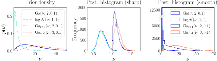
Figure 5: Prior and posterior of the degrees of freedom parameter $\nu$ (obtained using Gibbs). Left: different prior probability densities on $\nu$. Middle: posterior histograms of $\nu$ for the sharp signal. Right: posterior histograms of $\nu$ for the smooth signal.

Sampler comparison: Gibbs vs. NUTS. Using the prior distribution $\text{Ga}_{\nu>1}(\nu;\,2,0.1)$ on the degrees of freedom parameter $\nu$, we compare posterior statistics of $\nu$ obtained using the Gibbs sampler with those obtained via the NUTS sampler. In NUTS, we follow the standard Student’s $t$ formulation $\mathcal{T}_{\nu}\left(\mu,\tau^{2}\right)$ with hyperpriors $\tau^{2}\sim\text{IG}(1,10^{-4})$ and $\nu\sim\text{Ga}_{\nu>1}(2,0.1)$ as described in Section 4.2. We run NUTS sampler to obtain $n_{s}=2\times 10^{4}$ states and apply additionally burn-in of $n_{b}=2\times 10^{3}$.

Signal reconstructions are of the same good quality when either Gibbs or NUTS is used. In Figure 6, we compare the posterior statistics for the parameter $\nu$ obtained using both samplers for the sharp signal. Since the posterior chains are comparatively good, we can conclude that the Gibbs sampler is exploring the target posterior distribution. We omit the analogous chain plot for the smooth signal scenario in the sake of brevity. However, we note that inference of the $\nu$ parameter is more challenging in the smooth signal case, as the Gibbs chain has slightly more correlation than the one computed by NUTS. Nonetheless, we remark here that the main advantage of the Gibbs sampler over NUTS is its independence from gradient computations.

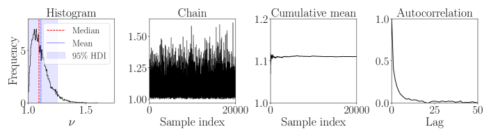
(a)

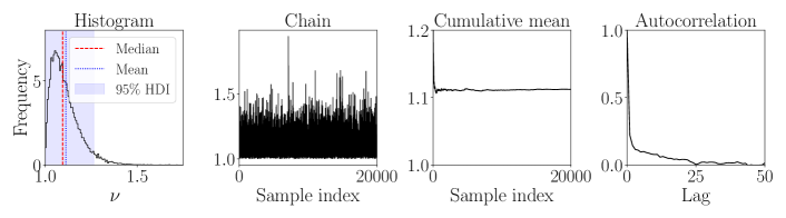
(b)

Figure 6: Posterior statistics of $\nu$ for the sharp signal obtained using NUTS (top) and Gibbs (bottom). Prior on $\nu$ is $\text{Ga}_{\nu>1}(2,0.1)$.

Prior comparison: Student’s $t$ prior vs. Laplace prior. We also compare posterior obtained with the Students’s $t$ prior with the posterior obtained using the Laplace prior [21]. In one-dimensional case, Laplace prior is equivalent to the total variation prior and is defined as

$$p(\bm{x})=\left(\frac{\delta}{2}\right)^{d}\exp\left(-\delta\|\bm{D}\bm{x}\|_{1}\right),$$ (32)

where the difference matrix $\bm{D}$ is defined in eq. 4, parameter $\delta\in\mathbb{R}_{>0}$ is the inverse scale, and $\left\|\cdot\right\|_{1}$ denotes the $\ell_{1}$-norm. We sample both cases using NUTS ($n_{s}=2\times 10^{4}$ states with additional burn-in $n_{b}=2\times 10^{3}$).

In Figure 7, we show posterior statistics of parameter $\bm{x}$. In the smooth signal test, both prior behave comparatively well resulting in small relative error and similar uncertainty. However, in the piecewise constant case, our Student’s $t$ prior improves the reconstruction error and reduces the posterior uncertainty.

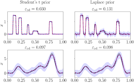
Figure 7: Comparison of posterior statistics for the target parameter $\bm{x}$ using NUTS. Left: Student’s $t$ prior. Right: Laplace prior. Results are shown for the sharp signal (top row) and smooth signal (bottom row). True solution (black solid line), posterior median (red dashed line), posterior mean (blue dotted line), and $95\%$ highest density interval (shaded area).

5.2 Image deblurring

In image deblurring, we aim at recovering the original sharp image from the corresponding noisy blurred image using a mathematical model of the blurring process.

If we denote the image domain by $\mathcal{D}=([0,1]\times[0,1])$, and $\bm{t}=[t_{1},t_{2}]^{\mathsf{T}}\in\mathcal{D}$, $\bm{s}=[s_{1},s_{2}]^{\mathsf{T}}\in\mathcal{D}$ then the blurred image $y$ can be obtained from the true image $x$ using the Fredholm integral operator as follows [53]

$$y(\bm{t})=\int_{\mathcal{D}}\mathcal{A}(\bm{t},\bm{s})x(\bm{s})d\bm{s}\quad\mathrm{with}\quad\mathcal{A}(\bm{t},\bm{s})=\frac{1}{2\pi\sigma^{2}}\exp\left(-\frac{(t_{1}-s_{1})^{2}+(t_{2}-s_{2})^{2}}{2\sigma^{2}}\right),$$ (33)

where $\mathcal{A}(\bm{t},\bm{s})$ is the Gaussian convolution kernel specifying the blurring (similar to the one-dimensional case).

As a true image, we use a square-and-disk phantom of size $64\times 64$, that is, $N=64$, and the problem dimension is $d=N^{2}=4\,096$ [2]. We generate blurred image (of the same size) using the blurring model eq. 33 with parameter $\sigma=6$ and standard deviation $\sigma_{\mathrm{obs}}^{\mathrm{true}}=3.3\times 10^{-3}$. The true image and its noisy blurry version are shown in Figure 8.

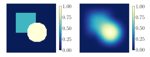
Figure 8: Image deblurring example. Left: underlying true image (square-and-disk phantom). Right: corresponding noisy blurred image (1% relative noise).

We estimate posterior under Student’s $t$ prior (with $\nu\sim\text{Ga}_{\nu>1}(\nu;\,2,0.1)$) using the Gibbs sampler. Next, we compare results with those obtained by NUTS with Laplace MRF prior that is defined in two-dimensional case as follows

$$p(\bm{x})=\left(\frac{\delta}{2}\right)^{d}\exp\left[-\delta\left(\|\bm{D}^{(1)}\bm{x}\|_{1}+\|\bm{D}^{(2)}\bm{x}\|_{1}\right)\right],$$ (34)

where difference matrices $\bm{D}^{(1)}$ and $\bm{D}^{(2)}$ are horizontal and vertical difference matrices, parameter $\delta\in\mathbb{R}_{>0}$ is the inverse scale, and $\left\|\cdot\right\|_{1}$ denotes the $\ell_{1}$-norm.

The input parameters to the Gibbs and NUTS samples are the same as in one-dimensional deconvolution example. In Figure 9, we show posterior mean and logarithm of standard deviation for two deblurred images obtained with Student’s $t$ prior and Laplace prior. We plot the logarithm of standard deviation to facilitate the interpretation for the Student’s $t$ prior, as maximum values of standard deviation occur at single pixels of the image. We note for Student’s $t$ prior the minimum value of the standard deviation is $1.286\times 10^{-4}$ and the maximum value is $0.041$ (if we omit two points exhibiting larger standard deviation values of $0.639$ and $0.675$). Whereas, for Laplace prior the standard deviation ranges from $0.128$ to $0.259$.

The relative reconstruction error is $0.218$ for Student’s $t$ and $0.215$ for Laplace. Despite both priors yield comparable relative errors, we can clearly see that the mean of posterior based on Student’s $t$ prior is sharper, contains less noise and has smaller posterior uncertainty. It can be also noted that for the Laplace prior the larger values of standard deviation are located at the edges pointing to the higher uncertainty in the boundary regions.

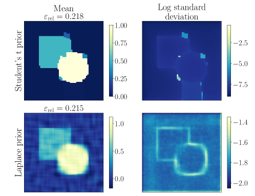
Figure 9: Comparison of posterior statistics for the target parameter $\bm{x}$ using the Student’s $t$ prior (top row) and the Laplace prior (bottom row). Posterior mean with relative error $\varepsilon_{\mathrm{rel}}$ (left) and logarithm of the standard deviation (right).

In addition, for Student’s $t$ , we report posterior statistics of the local scale parameter $\bm{w}$ in Figure 10, and chain statistics of scalar parameters (degrees of freedom $\nu$ and the global scale $\tau$) in Figure 11. In the Laplace prior case, the posterior mean and standard deviation of the inverse scale parameter $\delta$ are $3.214$ and $0.151$, respectively.

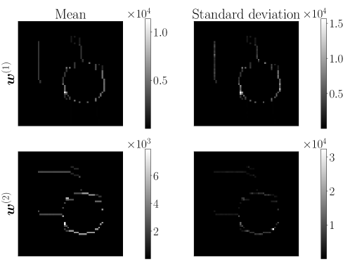
Figure 10: Posterior mean (left) and standard deviation (right) of the local scale parameter $\bm{w}$ obtained under the Student’s $t$ prior using Gibbs. Top row: horizontal components $\bm{w}^{(1)}$, bottom row: vertical components $\bm{w}^{(2)}$.

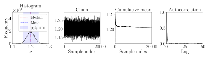
(a)

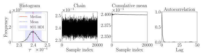
(b)

Figure 11: Posterior statistics for $\nu$ (top row) and $\tau$ (bottom row), obtained under the Student’s $t$ prior using Gibbs: histogram, chain, cumulative mean and sample autocorrelation.

6 Summary and conclusions

We developed a computational framework for solving linear Bayesian inverse problems in which the unknown can be either discontinuous or smooth. Our method involves flexible priors based on Markov random fields combined with Student’s $t$ distribution. We solve a hierarchical Bayesian inverse problem that allows joint estimation of the degrees of freedom parameter of the Student’s $t$ distribution. Flexible estimation of degrees of freedom provides an opportunity to tailor the prior for recovering not only sharp but also smooth features depending on the task.

Due to the hierarchical structure and the Student’s $t$ distributions involved in the prior, sampling of the posterior distribution is challenging. To address the issue, we employed a Gaussian scale mixture representation of the Student’s $t$ distribution, that allowed us to employ an efficient Gibbs sampler. We validated numerically our suggested Gibbs sampler by comparing its results to the solution obtained via NUTS.

In the numerical experiments, we showed that Student’s $t$ hierarchical prior can be applied for recovering blocky objects as well as the objects containing smooth features. To access the performance of the proposed method in Bayesian inversion, we compared Student’s $t$ priors with more traditional prior models based on Laplace Markov random fields commonly used for promoting sharp features. As compared to Laplace priors, Student’s $t$ priors enable the computation of sharp point estimates of the posterior while reducing the posterior uncertainty.

As a future work, we consider employing a higher-order difference matrix in the MRF structure to add more structural dependencies. This could be potentially beneficial for the smooth case scenario as opposed to our current implementation based on the first-order difference matrix, which models connections in the two neighbouring pixels only. In addition, we would like to extend the method to the higher dimensional inverse problems. This essentially requires application of efficient methods to sample from high-dimensional Gaussian distributions.

References

- Tarantola [2004] A. Tarantola, Inverse Problem Theory and Methods for Model Parameter Estimation, Society for Industrial and Applied Mathematics, USA, 2004.
- Hansen [2010] P. C. Hansen, Discrete Inverse Problems: Insight and Algorithms, Society for Industrial and Applied Mathematics (SIAM), 2010.
- Marzouk and Najm [2009] Y. M. Marzouk, H. N. Najm, Dimensionality reduction and polynomial chaos acceleration of Bayesian inference in inverse problems, Journal of Computational Physics 228 (2009).
- Cui et al. [2014] T. Cui, J. Martin, Y. M. Marzouk, A. Solonen, A. Spantini, Likelihood-informed dimension reduction for nonlinear inverse problems, Inverse Problems 30 (2014) 0114015.
- Uribe et al. [2021] F. Uribe, I. Papaioannou, J. Latz, W. Betz, E. Ullmann, D. Straub, Bayesian inference with subset simulation in varying dimensions applied to the Karhunen–Loève expansion, International Journal for Numerical Methods in Engineering 122 (2021) 5100–5127.
- Kaipio and Somersalo [2005] J. Kaipio, E. Somersalo, Statistical and Computational Inverse Problems, Springer, 2005.
- Bardsley [2019] J. M. Bardsley, Computational Uncertainty Quantification for Inverse Problems, Society for Industrial and Applied Mathematics (SIAM), 2019.
- Andrews and Mallows [1974] D. F. Andrews, C. L. Mallows, Scale mixtures of normal distributions, Journal of the Royal Statistical Society: Series B (Methodological) 36 (1974) 99–102.
- Geman and Geman [1984] S. Geman, D. Geman, Stochastic relaxation, Gibbs distributions, and the Bayesian restoration of images, IEEE Transactions on Pattern Analysis and Machine Intelligence PAMI-6 (1984) 721–741.
- Robert and Casella [2004] C. P. Robert, G. Casella, Monte Carlo Statistical Methods, 2 Edition., Springer, 2004.
- Müller [1991] P. Müller, A generic approach to posterior integration and Gibbs sampling, Technical Report #91-09, Department of Statistics, Purdue University, 1991.
- Geweke [1993] J. Geweke, Bayesian treatment of the independent Student-t linear model, Journal of Applied Econometrics 8 (1993) S19–S40.
- Fernandez and Steel [1998] C. Fernandez, M. F. J. Steel, On Bayesian modeling of fat tails and skewness, Journal of the American Statistical Association 93 (1998) 359–371.
- Fonseca et al. [2008] T. C. O. Fonseca, M. A. R. Ferreira, H. S. Migon, Objective Bayesian analysis for the Student-t regression model, Biometrika 95 (2008) 325–333.
- Juárez and Steel [2010] M. Juárez, M. Steel, Model-based clustering of non-Gaussian panel data based on skew-t distributions, Journal of Business & Economic Statistics 28 (2010) 52–66.
- Simpson et al. [2017] D. Simpson, H. Rue, A. Riebler, T. G. Martins, S. H. Sørbye, Penalising Model Component Complexity: A Principled, Practical Approach to Constructing Priors, Statistical Science 32 (2017) 1 – 28.
- He et al. [2021] D. He, D. Sun, L. He, Objective Bayesian analysis for the Student-t linear regression, Bayesian Analysis 16 (2021) 129–145.
- Lee [2022] S. Y. Lee, The use of a log-normal prior for the Student t-distribution, Axioms 11 (2022).
- Bardsley [2013] J. M. Bardsley, Gaussian Markov random field priors for inverse problems, Inverse Problems and Imaging 7 (2013) 397–416.
- Roininen et al. [2014] L. Roininen, J. M. J. Huttunen, S. Lasanen, Whittle-Matérn priors for Bayesian statistical inversion with applications in electrical impedance tomography, Inverse Problems and Imaging 8 (2014) 561–586.
- Bardsley [2012] J. M. Bardsley, Laplace-distributed increments, the Laplace prior, and edge-preserving regularization, Journal of Inverse and Ill-Posed Problems 20 (2012) 271–285.
- Suuronen et al. [2022] J. Suuronen, N. K. Chada, L. Roininen, Cauchy Markov random field priors for Bayesian inversion, Statistics and Computing 32 (2022) 1573–1375.
- Senchukova et al. [2023] A. Senchukova, J. Suuronen, J. Heikkinen, L. Roininen, Geometry parameter estimation for sparse X-ray log imaging, Journal of Mathematical Imaging and Vision 66 (2023) 154–166.
- Suuronen et al. [2023] J. Suuronen, T. Soto, N. K. Chada, L. Roininen, Bayesian inversion with -stable priors, Inverse Problems 39 (2023) 105007.
- Uribe et al. [2023] F. Uribe, Y. Dong, P. C. Hansen, Horseshoe priors for edge-preserving linear Bayesian inversion, SIAM Journal on Scientific Computing 45 (2023) B337–B365.
- Calvetti and Somersalo [2007] D. Calvetti, E. Somersalo, A Gaussian hypermodel to recover blocky objects, Inverse problems 23 (2007) 733–754.
- Calvetti and Somersalo [2008] D. Calvetti, E. Somersalo, Hypermodels in the Bayesian imaging framework, Inverse problems 24 (2008) 034013 (20pp).
- Calvetti et al. [2020] D. Calvetti, M. Pragliola, E. Somersalo, A. Strang, Sparse reconstructions from few noisy data: Analysis of hierarchical Bayesian models with generalized gamma hyperpriors, Inverse Problems 36 (2020) 025010.
- Chu [1973] K.-C. Chu, Estimation and decision for linear systems with elliptical random processes, IEEE Transactions on Automatic Control 18 (1973) 499–505.
- Choy and Smith [1997] S. T. B. Choy, A. F. M. Smith, Hierarchical models with scale mixtures of normal distributions, Test 6 (1997).
- Hoffman and Gelman [2014] M. D. Hoffman, A. Gelman, The No-U-Turn Sampler: Adaptively setting path lengths in Hamiltonian Monte Carlo, Journal of Machine Learning Research 15 (2014) 1593–1623.
- Tenorio [2017] L. Tenorio, An Introduction to Data Analysis and Uncertainty Quantification for Inverse Problems, Society for Industrial and Applied Mathematics (SIAM), 2017.
- Spanos and Ghanem [1989] P. Spanos, R. Ghanem, Stochastic finite element expansion for random media, Journal of Engineering Mechanics 115 (1989) 1035–1053.
- Lassas et al. [2009] M. Lassas, E. Saksman, S. Siltanen, Discretization-invariant Bayesian inversion and Besov space priors, Inverse Problems & Imaging 3 (2009) 87–122.
- Li et al. [2022] C. Li, M. Dunlop, G. Stadler, Bayesian neural network priors for edge-preserving inversion, Inverse Problems and Imaging 0 (2022) 1–26.
- Rue and Held [2005] H. Rue, L. Held, Gaussian Markov Random Fields. Theory and Applications, Chapman & Hall/CRC, 2005.
- Samorodnitsky and Taqqu [1994] G. Samorodnitsky, M. S. Taqqu, Stable Non-Gaussian Random Processes: Stochastic Models With Infinite Variance, Chapman and Hall/CRC, 1994.
- West [1987] M. West, On scale mixtures of normal distibutions, Biometrika 74 (1987) 646–648.
- Feller [1971] W. Feller, An Introduction to Probability Theory and Its Applications, Vol. 2, 2 Edition., Wiley, 1971.
- Wainwright and Simoncelli [1999] M. J. Wainwright, E. Simoncelli, Scale mixtures of Gaussians and the statistics of natural images, in: Advances in Neural Information Processing Systems, volume 12, MIT Press, 1999.
- Higdon [2007] D. Higdon, A primer on space-time modeling from a Bayesian perspective, in: Statistical Methods for Spatio-Temporal Systems, Chapman & Hall/CRC, 2007, pp. 217–279.
- Calvetti et al. [2020] D. Calvetti, M. Pragliola, E. Somersalo, Sparsity promoting hybrid solvers for hierarchical Bayesian inverse problems, SIAM Journal on Scientific Computing 42 (2020) A3761–A3784.
- Law and Zankin [2022] K. J. H. Law, V. Zankin, Sparse online variational Bayesian regression, SIAM/ASA Journal on Uncertainty Quantification 10 (2022) 1070–1100.
- Villa and Walker [2013] C. Villa, S. Walker, Objective prior for the number of degrees of freedom of a t distribution, Bayesian Analysis 9 (2013) 1–24.
- Cotter et al. [2013] S. Cotter, G. Roberts, A. Stuart, A. White, MCMC methods for functions: Modifying old algorithms to make them faster, Statistical Science 28 (2013) 424–446.
- Gamerman and Lopes [2006] D. Gamerman, H. F. Lopes, Markov Chain Monte Carlo: Stochastic Simulation for Bayesian Inference, 2 Edition., Chapman and Hall/CRC, 2006.
- Andrieu and Thoms [2008] C. Andrieu, J. Thoms, A tutorial on adaptive MCMC, Statistics and Computing 18 (2008) 343–373.
- Besag [1974] J. Besag, Spatial interaction and the statistical analysis of lattice systems, Journal of the Royal Statistical Society. Series B (Methodological) 36 (1974) 192–236.
- Roberts and Smith [1994] G. O. Roberts, A. F. M. Smith, Simple conditions for the convergence of the Gibbs sampler and Metropolis-Hastings algorithms, Stochastic Processes and their Applications 49 (1994) 207–216.
- Tierney [1994] L. Tierney, Markov chains for exploring posterior distributions, The Annals of Statistics 22 (1994) 1701–1762.
- Owen [2023] A. B. Owen, Monte Carlo Theory, Methods and Examples, artowen.su.domains/mc/, 2023.
- Petersen and Pedersen [2012] K. B. Petersen, M. S. Pedersen, The matrix cookbook, 2012. URL: http://www2.compute.dtu.dk/pubdb/pubs/3274-full.html, version 20121115.
- Lu et al. [2010] Y. Lu, L. Shen, Y. Xu, Integral equation models for image restoration: High accuracy methods and fast algorithms, Inverse Problems 26 (2010) 045006.