Priority-based Energy Allocation in Buildings for Distributed Model Predictive Control

Abstract

Many countries are facing energy shortage today and most of the global energy is consumed by HVAC systems in buildings. For the scenarios where the energy system is not sufficiently supplied to HVAC systems, a priority-based allocation scheme based on distributed model predictive control is proposed in this paper, which distributes the energy rationally based on priority order. According to the scenarios, two distributed allocation strategies, i.e., one-to-one priority strategy and multi-to-one priority strategy, are developed in this paper and validated by simulation in a building containing three zones and a building containing 36 rooms, respectively. Both strategies fully exploit the potential of predictive control solutions. The experiment shows that our scheme has good scalability and achieve the performance of centralized strategy while making the calculation tractable.

Note to Practitioners

Renewable energy systems are increasingly popular worldwide, but their energy reserves are limited by natural conditions (e.g., solar, wind). The motivation of this paper is to develop a priority-based allocation strategy adapted to renewable energy systems. When energy is limited, the strategy is able to rationally allocate energy and satisfy the urgent need energy supply in some specific zones. Two priority strategies are proposed for the case of one-to-one correspondence between priorities and subsystems and multiple subsystems corresponding to the same priority, respectively. The developed strategies have been validated by co-simulation with MATLAB and EnergyPlus in a small-scale 3-zone building and a large-scale 36-zone building to show its effectiveness.

I Introduction

The building sector accounts for more than 40% of global energy consumption [1, 2], and more than 1/3 of carbon emissions are contributed by this sector [3, 4]. Under the United Nations Framework Convention on Climate Change (UNFCCC), China has committed to peak CO₂ emissions with a target date of 2030, announcing that it will reduce CO₂ emissions per unit of gross domestic product by 60–65% of the emission levels in 2005 [5, 6]. Heating, Ventilation and Air Conditioning (HVAC) systems are the main consumers of energy in buildings, which makes them suitable candidates for improving building energy efficiency and reducing energy consumption, thus contributing to limiting global carbon emissions. Well-designed control rules applied to the building HVAC module offer a promising approach to improving the building energy efficiency.

Due to the advantages of low cost, simple operation and easy implementation, traditional control methods are still used in a large number of buildings to control HVAC systems [7, 8], including manual control, feedback control, feed-forward control, PID control and so on. However, the control parameters of traditional methods are difficult to adjust and cannot handle the nonlinear dynamics of the system, which often leads to overshooting and makes the building operation inefficient. [9] proposes a hybrid particle swarm optimization algorithm for optimal tuning of conventional PID controllers and compares this method with the Ziegler-Nichols method, but this method is still not able to deal with the nonlinear dynamics and disturbances of the HVAC system. In order to deal with the nonlinear dynamics of the building, rule-based control methods have been developed, which are based on a series of “if-then-else” rules written based on expert experience or a priori knowledge to control the HVAC system. [10, 11] have achieved good control results using rule-based control methods. Although these rule-based methods can take into account the real-time constraints and nonlinearities of the system and do improve the energy efficiency of the system, they lack global optimization of the system and the rules are complex to write and maintain. As a result, these approaches require a great deal of experience and expertise in practical implementation and are difficult to generalise and replicate.

In recent years, model predictive control (MPC) has received considerable attention from researchers as a promising advanced control method. In addition to well-known advantages of dealing with nonlinear dynamic models and constraints in a systematic mode, MPC controllers could take into account weather forecasts, room occupancy, and other information that may be relevant to the optimal control law of the system during operation. However, as the scale of the building complex increases, the complexity of the system’s dynamic model increases. In this case, the number of decision variables to be processed by the MPC controller during each execution becomes very large, and limited computational power makes it difficult to deploy centralized MPC controllers in large-scale building systems.

Large-scale, multi-coupled and multi-constraint complex systems can be effectively handled by distributed model predictive control (Distributed MPC), which is a suitable method for managing energy distribution in buildings, especially when the number of control variables and signals from sensors grows rapidly with the scale of the HVAC system. In addition to building sector, its application areas involve other engineering systems such as traffic control [12], smart grids [13], water supply systems [14], supply chains [15], floating object transport [16], unmanned aerial vehicle formations [17], vehicle formations [18], etc.

Distributed MPC splits the original centralized problem into multiple local subproblems, which are small and easy to solve. Coordination of the local subproblems can be performed locally through communication between the subproblems or through a global coordinator. The distributed control technique is not significantly affected by the number of HVAC systems, so many scholars have started to investigate distributed techniques applied to large-scale buildings. [19] proposes a method based on dual decomposition for co-optimising buildings and energy hubs to improve energy efficiency and conservation. A distributed MPC framework based on Benders decomposition is illustrated in [20] for controlling a building heating system consisting of a central heat source and multiple local heat sources. A limited communication distributed model predictive control (LC-DMPC) algorithm for coupled and constrained linear discrete systems is proposed in [21]. [22] invokes the new concept of grid aggregator in the LC-DMPC structure and extends the algorithm to enable buildings to interact with the grid. Nash equilibrium and alternating direction method of multipliers (ADMM) is used in [23] to coordinate the control inputs in each zone.

In this paper, we propose a priority-based distributed scheme to rationally allocate building energy, which skillfully decouples the subsystems. The advantage of this approach is that instead of solving the global optimization problem, the optimization problem containing only the subsystem’s own objective function and constraints are solved in parallel with a small communication cost.

The contributions of this paper are as follows.

• Different from other literatures devoted to the study of how to save energy under abundant energy supply, the focus of this paper is not only on energy saving, but also on the proper distribution of limited energy.

• For a limited amount of energy, it is not possible to make all the rooms satisfy the comfort requirements. The contribution of this paper is to provide a distributed scheme that allocates energy according to priority to satisfy the energy supply of the rooms that are in urgent need of energy supply. The algorithm is independent of the size of the system and is scalable. Optimization operations could be performed by subsystems in parallel.

• Priority-based allocation algorithm in this paper exploits the potential of predictive control solutions, i.e., it utilises all the solutions obtained by predictive control. In contrast, the original predictive control would only use the first element of the solution sequence and discard the other elements.

• Few literatures have considered really large scale cases, the algorithm proposed in this paper is applied to consider a large scale scenario energy distribution for 36 zones. Simulation experiments illustrate that the proposed algorithm is well suited for application in large-scale scenarios.

II System description

II-A Overview

The work in this paper is to rationally allocate energy to the zones based on MPC according to the priority order. Fig. 1 shows the overall framework of the scheme in this paper. The control algorithm is deployed in MATLAB and the resistance-capacitance (RC) model is employed as the prediction model for predictive control. An optimization operation that considers building occupancy information, weather forecasts and local electricity prices yields the HVAC set point. The control action is then applied via Mle+ [24] to the building model developed in EnergyPlus [25]. After each optimization operation, the real-time states of the building in EnergyPlus are updated to MATLAB via Mle+ for the next optimization implementation.

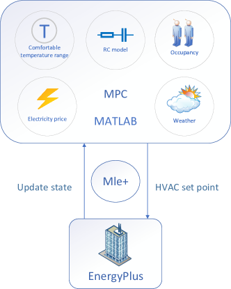
Figure 1: Framework of energy allocation.

II-B Prediction model for MPC

The RC model is a commonly used prediction model in the building sector, which is built based on indoor nodes and wall nodes. Notations of the quantities in this section is shown in Table I.

TABLE I: Notations of the quantities

Notation	Description
$ori$	Take the values $n$, $e$, $w$ and $s$, representing north, east, west, and south
$ori2$	Take the values $n$, $e$, $w$ and $s$, but $ori\neq ori2$
$u$	Output power of HVAC systems
$C_{z}$	Thermal capacity of the zone
$C_{{ori}}^{w}$	Thermal capacity of the wall
$R_{ori}^{w}$	Thermal resistance for conduction of the wall
$R_{ori}$	Thermal resistance for convection on inside surface
$R_{ori}^{\prime}$	Thermal resistance for convection on outside surface
$T_{z}$	Indoor air temperature
$T_{ori}^{out}$	Outside temperature adjacent to the $ori$ wall
$T_{ori2}^{out}$	Outside temperature adjacent to the $ori2$ wall
$T_{ori}^{wi}$	Inside surface temperature of the $ori$ wall
$T_{ori}^{wo}$	Outside surface temperature of the $ori$ wall
$T_{out}$	Outdoor ambient temperature
$\dot{Q}_{ori}^{rad}$	Solar radiation, $ori$ wall
$\dot{Q}_{ori2}^{rad}$	Solar radiation, $ori2$ wall
$\dot{Q}_{z}^{in}$	Internal gains in the zone
$\dot{Q}_{z}^{rad}$	Solar radiation in the zone

For the zone, the differential equation about the indoor node is

$$\begin{aligned} C_{z}\frac{dT_{z}}{dt}=&\frac{T_{n}^{wi}-T_{z}}{R_{n}}+\frac{T_{e}^{wi}-T_{z}}{R_{e}}+\frac{T_{w}^{wi}-T_{z}}{R_{w}}\\ &+\frac{T_{s}^{wi}-T_{z}}{R_{s}}+u+\dot{Q}_{z}^{in}+\dot{Q}_{z}^{rad}\end{aligned}.$$ (1)

The differential equation for the inside surface of the wall in the $ori$ direction is

$$C_{{ori}}^{w}\frac{dT_{{ori}}^{wi}}{dt}=\frac{T_{z}-T_{{ori}}^{wi}}{R_{{ori}}}+\frac{T_{{ori}}^{wo}-T_{{ori}}^{wi}}{R_{{ori}}^{w}}.$$ (2)

The differential equation for the outside surface of the wall in the $ori$ direction is

$$C_{{ori}}^{w}\frac{dT_{{ori}}^{wo}}{dt}=\frac{T_{{ori}}^{out}-T_{{ori}}^{wo}}{R_{{ori}}^{\prime}}+\frac{T_{{ori}}^{wi}-T_{{ori}}^{wo}}{R_{{ori}}^{w}}+\dot{Q}_{{ori}}^{{rad}}.$$ (3)

The RC model of the zone is established and discretized as

$$\begin{aligned} {x}(k+1)&=Ax(k)+B_{u}u(k)+B_{d}d(k)\\ y(k)&=Cx(k)\end{aligned}.$$ (4)

The state variable of the system is composed of the indoor air temperature in the zone and the inside and outside surface temperatures of the four oriented walls in the zone, i.e., $x=[\begin{array}[]{ll}T_{z}&T_{w}^{wi}\end{array}$ $\begin{array}[]{lllllll}T_{n}^{wi}&T_{e}^{wi}&T_{s}^{wi}&T_{w}^{wo}&T_{n}^{wo}&T_{e}^{wo}&T_{s}^{wo}\end{array}]^{T}$ $\in\mathbb{R}^{9}$. The system input is $u\in\mathrm{R}$, and disturbances are $d=[\begin{array}[]{ll}T_{out}&T_{ori}^{out}\end{array}$ $\begin{array}[]{lllllll}T_{ori2}^{out}&\dot{Q}_{ori}^{rad}&\dot{Q}_{ori2}^{rad}&\dot{Q}_{z}^{in}&\dot{Q}_{z}^{rad}\end{array}]^{T}\in\mathbb{R}^{7}$. $A$, $B_{u}$, and $B_{d}$ are the corresponding constant coefficient matrices. $y$ is the indoor air temperature, i.e. $\begin{array}[]{lllllllll}C=[1&0&0&0&0&0&0&0&0]\end{array}\in\mathbb{R}^{9}$.

The R-values and C-values in this paper are shown in Table II.For validation of the RC model and more details see [26].

TABLE II: R-values and C-values

Parameter	Value($J/K$)	Parameter	Value($K/W$)
$C_{z}$	$4.8\times 10^{4}$	$R_{e,w}$	0.0232
$C_{{n}}^{w}$	$8.5\times 10^{5}$	$R_{n,s}$	0.0310
$C_{{e}}^{w}$	$1.1\times 10^{6}$	$R_{e,w}^{w}$	0.0179
$C_{{w}}^{w}$	$1.1\times 10^{6}$	$R_{n,s}^{w}$	0.0238
$C_{{s}}^{w}$	$8.5\times 10^{5}$	$R_{e,w}^{\prime}$	0.0087
		$R_{n,s}^{\prime}$	0.0116

III Control methodologies

III-A Centralized MPC formulation

The centralized control strategy is to design a master controller to coordinate the temperature of all zones. The centralized block diagram for $n$ zones is shown in Fig. 2.

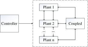
Figure 2: Centralized control framework.

The optimization objective function consists of three components: one is to impose a soft constraint to limit the room temperature; the second is to minimize the energy consumption; and the third is to control the action to be as gentle as possible to avoid the loss of components by excessive control actions. The scheme for centralized predictive control is designed as follows:

$$\begin{array}[]{lll}&\min\limits_{\begin{subarray}{c}\mathbf{u}_{1},\cdots,\mathbf{u}_{n}\\ \mathbf{v}_{1},\cdots,\mathbf{v}_{n}\end{subarray}}&J(k)=\sum\limits_{m\in\Phi}\theta_{m}[\alpha\sum\limits_{l=1}^{P}\left\|v_{m}(k+l)\right\|^{2}\cdot{\delta_{m}(k+l)}\\ &&\qquad\qquad+\sum\limits_{l=1}^{M}\left\|u_{m}(k+l-1)\right\|^{2}\cdot{\lambda_{m}(k+l-1)}]\\ &\text{ s.t. }&X(k+1)=AX(k)+B_{u}u(k)+B_{d}d(k)\\ &&y(k)=CX(k)\\ &&X(k)=X^{*}\\ &&\sum\limits_{m\in\Phi}\mathbf{u}_{m}\leq\mathbf{c}^{\max}\\ &&\text{ For all }m\in\Phi:\\ &&\mathbf{u}_{m}^{\min}\leq\mathbf{u}_{m}\leq\mathbf{u}_{m}^{\max}\\ &&\mathbf{y}_{m}^{\min}\leq\mathbf{y}_{m}+\mathbf{v}_{m}\\ &&\mathbf{y}_{m}^{\max}\geq\mathbf{y}_{m}-\mathbf{v}_{m}\\ &&\mathbf{v}_{m}\geq 0\\ \end{array}$$ (5)

where $\Phi$ is the set of all $n$ subsystems. $\alpha$ is the weight, which can be set according to the user’s preference (more energy efficient or more comfortable). $\theta$ is the weight that regulates the importance of energy levels between subsystems. $u$ denotes the output power of the HVAC system. $\delta$ takes the value of 1 when the building is occupied and 0 when the building is not occupied. Electricity charge rate in Shenzhen is shown in Table III, and $\lambda$ is the weight for the time-varying electricity price. The effect of $\mathbf{v}$ is to impose a soft constraint that allows the room temperature to be controlled to a suitable range. $X^{*}$ is the initial value of the state $X$ at $k$ moment. $\mathbf{c}^{\max}$ denotes the total energy limit.

TABLE III: Electricity charge rate in Shenzhen.

Time	Electricity price $\lambda$ (CNY/kWh)
0:00-8:00	0.3358
8:00-14:00	0.6629
14:00-17:00	1.0881
17:00-19:00	0.6629
19:00-22:00	1.0881
22:00-24:00	0.6629

III-B Decentralized MPC formulation

In the decentralized scenario, each zone is configured with a subcontroller. Each subcontroller corresponds to a subsystem, and there are couplings between the subsystems, but the controllers are completely independent. The decentralized block diagram for $n$ zones is shown in Fig. 3.

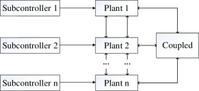
Figure 3: Decentralized control framework.

The decentralized MPC scheme for the $m$-th subsystem is as follows.

$$\begin{array}[]{lll}&\min\limits_{\mathbf{u}_{m},\mathbf{v}_{m}}&J_{m}(k)=\alpha\sum\limits_{l=1}^{P}\left\|v_{m}(k+l)\right\|^{2}\cdot{\delta_{m}(k+l)}\\ &&\qquad\qquad+\sum\limits_{l=1}^{M}\left\|u_{m}(k+l-1)\right\|^{2}\cdot{\lambda_{m}(k+l-1)}\\ &\text{ s.t. }&X_{m}(k+1)=A_{m}X_{m}(k)+B_{um}u_{m}(k)\\ &&\qquad\qquad\qquad+B_{dm}d_{m}(k)\\ &&y_{m}(k)=C_{m}X_{m}(k)\\ &&X_{m}(k)=X_{m}^{*}\\ &&\mathbf{u}_{m}\leq\hat{\mathbf{c}}^{a}\\ &&\mathbf{u}_{m}^{\min}\leq\mathbf{u}_{m}\leq\mathbf{u}_{m}^{\max}\\ &&\mathbf{y}_{m}^{\min}\leq\mathbf{y}_{m}+\mathbf{v}_{m}\\ &&\mathbf{y}_{m}^{\max}\geq\mathbf{y}_{m}-\mathbf{v}_{m}\\ &&\mathbf{v}_{m}\geq 0\\ \end{array}$$ (6)

where $\hat{\mathbf{c}}^{a}=1/n\cdot\mathbf{c}^{\max}$ and $n$ is the number of subsystems. Compared to centralized strategies, decentralized controllers deal with relatively simple optimization problems because the size of the objective function and constraints are reduced. However, the decentralized strategy is not flexible enough to handle the shared constraints and has insufficient scheduling capability for energy, which may result in insufficient supply for some rooms with high energy demand and energy redundancy for other rooms with low energy demand.

III-C Distributed algorithm

III-C1 Distributed MPC formulation

With a distributed strategy, there is an exchange of information between a subcontroller and its neighbor subcontrollers. The controller makes better decisions by combining the information obtained from the neighbors. The distributed control framework is shown in Fig. 4.

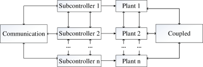
Figure 4: Distributed control framework.

The distributed MPC scheme for subsystem $m$ is as follows.

$$\begin{array}[]{lll}&\min\limits_{\mathbf{u}_{m},\mathbf{v}_{m}}&J_{m}(k)=\alpha\sum\limits_{l=1}^{P}\left\|v_{m}(k+l)\right\|^{2}\cdot{\delta_{m}(k+l)}\\ &&\qquad\qquad+\sum\limits_{l=1}^{M}\left\|u_{m}(k+l-1)\right\|^{2}\cdot{\lambda_{m}(k+l-1)}\\ &\text{ s.t. }&X_{m}(k+1)=A_{m}X_{m}(k)+B_{um}u_{m}(k)\\ &&\qquad\qquad\qquad+B_{dm}d_{m}(k)\\ &&y_{m}(k)=C_{m}X_{m}(k)\\ &&X_{m}(k)=X_{m}^{*}\\ &&\mathbf{u}_{m}\leq\hat{\mathbf{c}}_{m}(k)\\ &&\mathbf{u}_{m}^{\min}\leq\mathbf{u}_{m}\leq\mathbf{u}_{m}^{\max}\\ &&\mathbf{y}_{m}^{\min}\leq\mathbf{y}_{m}+\mathbf{v}_{m}\\ &&\mathbf{y}_{m}^{\max}\geq\mathbf{y}_{m}-\mathbf{v}_{m}\\ &&\mathbf{v}_{m}\geq 0\\ \end{array}$$ (7)

The value of $\mathbf{c}_{m}(k)$ is the key to solving the problem, and the following section describes how to get a reasonable $\mathbf{c}_{m}(k)$.

III-C2 One-to-one priority strategy

One-to-one priority means that each subsystem in the system corresponds to a different priority, i.e., $n$ subsystems correspond to $n$ priorities. The information exchange between subsystems in the one-to-one priority case is shown in Fig. 5, where the subsystems are numbered from 1 according to the priority of energy distribution, and the top-numbered subsystem has a high priority for energy supply. For subsystem $m$, it is defined that subsystem $m-1$ is the upstream subsystem and subsystem $m+1$ is the downstream subsystem. $\hat{\mathbf{c}}_{m}$ satisfies $\hat{\mathbf{c}}_{m+1}=\hat{\mathbf{c}}_{m}-\mathbf{u}_{m}$. For the first subsystem, the maximum energy limit is obtained, i.e. $\hat{\mathbf{c}}_{1}=\mathbf{c}^{max}$.

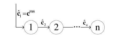
Figure 5: Information exchange between subsystems.

The subcontrollers of all subsystems can work in parallel. At moment $k$, subsystem $m$ gets $\hat{\mathbf{c}}_{m}(k)$ from the upstream subsystem $m-1$, then solves its own optimization problem and gets the solution $\mathbf{u}_{m}(k|k)$. Further, $\hat{\mathbf{c}}_{m+1}(k+1)$ is obtained by

$$\hat{\mathbf{c}}_{m+1}(k+1)=\hat{\mathbf{c}}_{m}(k+1|k)-\mathbf{u}_{m}(k+1|k),$$ (8)

and is transmitted to the downstream subsystem $m+1$. Remove the first element of $\mathbf{u}_{m}(k|k)$ and move the remaining elements one unit forward to get $\mathbf{u}_{m}(k+1|k)$. Note that the last two elements of $\mathbf{u}_{m}(k+1|k)$ are the same in order to keep the vector length consistent. The quantities of $\mathbf{u}_{m}$ and $\mathbf{c}_{m}$ are shown in (9). See Algorithm 1 for the one-to-one allocation algorithm. $K$ denotes the termination moment.

$$\begin{array}[]{c}\mathbf{u}_{m}(k|k)=[u_{m}(k|k)\quad u_{m}(k+1|k)\quad\cdots\quad u_{m}(k+M-1|k)]^{T}\\ \mathbf{u}_{m}(k+1|k)=[u_{m}(k+1|k)\quad u_{m}(k+2|k)\quad\cdots\quad u_{m}(k+M-1|k)\quad u_{m}(k+M-1|k)]^{T}\\ \hat{\mathbf{c}}_{m}(k)=[\hat{c}_{m}(k|k)\quad\hat{c}_{m}(k+1|k)\quad\cdots\quad\hat{c}_{m}(k+M-1|k)]^{T}\\ \hat{\mathbf{c}}_{m}(k+1|k)=[\hat{c}_{m}(k+1|k)\quad\hat{c}_{m}(k+2|k)\quad\cdots\quad\hat{c}_{m}(k+M-1|k)\quad\hat{c}_{m}(k+M-1|k)]^{T}\\ \end{array}$$ (9)

Algorithm 1 One-to-One Priority algorithm

1:Given the initial $\hat{\mathbf{c}}_{1},\cdots,\hat{\mathbf{c}}_{n}$.

2:for $k\in\{1,\cdots,K\}$ do

3:     parfor $m\in\Phi$ do

4:         Get $\hat{\mathbf{c}_{m}}(k)$ from upstream subsystem $m-1$.

5:         Solve (7) to obtain the solution $\mathbf{u}_{m}(k|k)$.

6:         Get $\mathbf{u}_{m}(k+1|k)$ and $\hat{\mathbf{c}}_{m}(k+1|k)$.

7:         Get $\hat{\mathbf{c}}_{m+1}(k+1)=\hat{\mathbf{c}}_{m}(k+1|k)-\mathbf{u}_{m}(k+1|k)$

8:   and transmit it to the downstream subsystem $m+1$.

9:     end parfor

10:end for

It is noted that the above computational process uses the predicted solution of the current moment for the future moment, so the distributed approach allows all subsystems to work in parallel and the size of the optimization problem to be handled by each subsystem does not increase with the size of the system.

III-C3 Multi-to-One priority strategy

Multi-to-one priority means that multiple subsystems in a system can correspond to the same priority level. In large-scale building systems, there may be multiple zones corresponding to the same supply priority level, and the multiple-to-one priority strategy is suitable for this situation.

The information matrix $I_{nf}$ records the information about the remaining energy, and if the subsystem is divided into $o$ energy supply levels starting from level 1, then $I_{nf}$ can be expressed as,

$$I_{nf}=\left(\begin{array}[]{c}\frac{\mathbf{c}_{\max}}{N_{{Pri}=1}}\\ \frac{\mathbf{c}_{\max}-\sum\limits_{Pri=1}\mathbf{u}}{N_{{Pri}=2}}\\ \frac{\mathbf{c}_{\max}-\sum\limits_{Pri=1}\mathbf{u}-\sum\limits_{Pri=2}\mathbf{u}}{N_{Pri=3}}\\ \vdots\\ \frac{\mathbf{c}_{\max}-\sum\limits_{Pri<g}\mathbf{u}}{N_{pri=g}}\\ \vdots\\ \frac{\mathbf{c}_{\max}-\sum\limits_{Pri<N_{o}}\mathbf{u}}{N_{pri=N_{o}}}\end{array}\right),$$

where ${\rm Pri}$ represents priority, $\sum\limits_{Pri<g}\mathbf{u}$ denotes the sum of the solutions for subsystems with priority less than $g$, ${N_{pri=g}}$ indicates the number of subsystems with priority $g$. $I_{nf}$ has $N_{o}$ rows and $M$ columns, and the last two columns have the same elements. For subsystem $m$, if its priority $Pri=g$, then $\hat{\mathbf{c}}_{m}$ records its energy residual information, $\hat{\mathbf{c}}_{m}=I_{nf}(g)$, $1\leq g\leq o$, and is the element of the g-th row of $I_{nf}$.

As Fig. 6 shown, each subsystem visits $I_{nf}(k)$ at the $k$-th moment,

$$I_{nf}(k)=\left(\begin{array}[]{cccc}\frac{c_{\max}}{N_{{pri}=1}}&\frac{c_{\max}}{N_{{pri}=1}}&\cdots&\frac{c_{\max}}{N_{{pri}=1}}\\ \frac{c_{\max}-\sum\limits_{Pri=1}u(k|k-1)}{N_{{pri}=2}}&\frac{c_{\max}-\sum\limits_{Pri=1}u(k+1|k-1)}{N_{{pri}=2}}&\cdots&\frac{c_{\max}-\sum\limits_{Pri=1}u(k+M-2|k-1)}{N_{{pri}=2}}\\ \vdots&\vdots&\vdots&\vdots\\ \frac{c_{\max}-\sum\limits_{Pri<g}u(k|k-1)}{N_{pri=g}}&\frac{c_{\max}-\sum\limits_{Pri<g}u(k+1|k-1)}{N_{pri=g}}&\cdots&\frac{c_{\max}-\sum\limits_{Pri<g}u(k+M-2|k-1)}{N_{pri=g}}\\ \vdots&\vdots&\vdots&\vdots\\ \frac{c_{\max}-\sum\limits_{Pri<N_{o}}u(k|k-1)}{N_{pri=N_{o}}}&\frac{c_{\max}-\sum\limits_{Pri<N_{o}}u(k+1|k-1)}{N_{pri=N_{o}}}&\cdots&\frac{c_{\max}-\sum\limits_{Pri<N_{o}}u(k+M-2|k-1)}{N_{pri=N_{o}}}\end{array}\right).$$

the corresponding $\hat{\mathbf{c}}$ is obtained, and then the optimization problem is solved and $I_{nf}$ is updated using the new solution to obtain $I_{nf}(k+1)$.

$$I_{nf}(k+1)=\left(\begin{array}[]{cccc}\frac{c_{\max}}{N_{{pri}=1}}&\frac{c_{\max}}{N_{{pri}=1}}&\cdots&\frac{c_{\max}}{N_{{pri}=1}}\\ \frac{c_{\max}-\sum\limits_{Pri=1}u(k+1|k)}{N_{{pri}=2}}&\frac{c_{\max}-\sum\limits_{Pri=1}u(k+2|k)}{N_{{pri}=2}}&\cdots&\frac{c_{\max}-\sum\limits_{Pri=1}u(k+M-1|k)}{N_{{pri}=2}}\\ \vdots&\vdots&\vdots&\vdots\\ \frac{c_{\max}-\sum\limits_{Pri<g}u(k+1|k)}{N_{pri=g}}&\frac{c_{\max}-\sum\limits_{Pri<g}u(k+2|k)}{N_{pri=g}}&\cdots&\frac{c_{\max}-\sum\limits_{Pri<g}u(k+M-1|k)}{N_{pri=g}}\\ \vdots&\vdots&\vdots&\vdots\\ \frac{c_{\max}-\sum\limits_{Pri<N_{o}}u(k+1|k)}{N_{pri=N_{o}}}&\frac{c_{\max}-\sum\limits_{Pri<N_{o}}u(k+2|k)}{N_{pri=N_{o}}}&\cdots&\frac{c_{\max}-\sum\limits_{Pri<N_{o}}u(k+M-1|k)}{N_{pri=N_{o}}}\end{array}\right).$$

When ${N_{pri=1}}={N_{pri=2}}=\cdots={N_{pri=N_{o}}}=1$, it degenerates to the case of one-to-one priority. It is noted that this distributed algorithm makes full use of the whole set of solutions in the prediction horizon, where the first element is applied to the plant and the others are used to update the information matrix $I_{nf}$. See Algorithm 2 for the multi-to-one allocation algorithm.

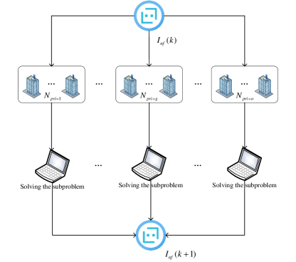
Figure 6: Information exchange for multi-to-one priority strategy.

Algorithm 2 Multi-to-One Priority algorithm

1:Given the initial $I_{nf}$.

2:for $k\in\{1,\cdots,K\}$ do

3:     Get $I_{nf}(k)$.

4:     parfor $m\in\Phi$ do

5:         Get $\hat{\mathbf{c}_{m}(k)}$ from $I_{nf}(k)$ according to the priority

6:   of $m$.

7:         Solve (7) to obtain the solution $\mathbf{u}_{m}(k|k)$.

8:         Get $\mathbf{u}_{m}(k+1|k)$.

9:     end parfor

10:     Update to $I_{nf}(k+1)$.

11:end for

III-D Strategic Analysis

III-D1 Optimization of the highest priority subsystems

Compared to the centralized scheme, in addition to reducing the problem size, our distributed scheme is similar to giving subsystems with higher priority a considerable weight in energy allocation, since the energy amount of subsystems with lower priority depends on the estimated residual energy of higher priority systems. We give a lemma and its proof to illustrate this statement.

Lemma 1

For optimizing $J_{1}$, the proposed distributed strategy perform better than or equal to the decentralized and centralized strategies.

Proof 1

Firstly, compare the optimization of the distributed and decentralised algorithms for $J_{1}$. Consider (6) with $\hat{\mathbf{c}}^{a}=1/n\cdot\mathbf{c}^{\max}$ and (7) with $\hat{\mathbf{c}}_{1}=\mathbf{c}^{max}$, we know that the feasible domain of the distributed problem (7) contains the feasible domain of the decentralised problem (6). Therefore, distributed strategy perform better than or equal to the decentralized strategy for optimizing $J_{1}$.

Then, compare the optimization of the distributed and centralised algorithms for $J_{1}$. The objective function of the centralized strategy is expressed as

$$\begin{array}[]{ll}J=&J_{1}\left(\mathbf{u}_{1},\mathbf{v}_{1}\right)+\frac{\theta_{2}}{\theta_{1}}J_{2}\left(\mathbf{u}_{2},\mathbf{v}_{2}\right)+\frac{\theta_{3}}{\theta_{1}}J_{3}\left(\mathbf{u}_{3},\mathbf{v}_{3}\right)\\ &+\cdots+\frac{\theta_{n}}{\theta_{1}}J_{n}\left(\mathbf{u}_{n},\mathbf{v}_{n}\right),\end{array}$$

where $\mathbf{u}_{1}+\mathbf{u}_{2}+\cdots+\mathbf{u}_{n}\leq\mathbf{c}_{\max}$ and $\theta_{1}\geq\theta_{2}\geq\cdots\geq\theta_{n}>0$. Since $J_{m}\geq 0$, optimizing $J_{1}$ alone is better or equal to optimizing $J$ for $J_{1}$. So the following optimization problem (10) is better or equal to the centralized strategy for optimizing $J_{1}$.

$$\begin{array}[]{lll}&\min\limits_{\mathbf{u}_{1},\mathbf{v}_{1}}&J_{1}(\mathbf{u}_{1},\mathbf{v}_{1})\\ &\text{ s.t. }&X_{1}(k+1)=A_{1}X_{1}(k)+B_{u1}u_{1}(k)\\ &&\qquad\qquad\qquad+B_{d1}d_{1}(k)\\ &&y_{1}(k)=C_{1}X_{1}(k)\\ &&X_{1}(k)=X_{1}^{*}\\ &&\mathbf{u}_{1}+\mathbf{u}_{2}+\cdots+\mathbf{u}_{n}\leq\mathbf{c}^{\max}\\ &&\mathbf{u}_{1}^{\min}\leq\mathbf{u}_{1}\leq\mathbf{u}_{1}^{\max}\\ &&\mathbf{y}_{1}^{\min}\leq\mathbf{y}_{1}+\mathbf{v}_{1}\\ &&\mathbf{y}_{1}^{\max}\geq\mathbf{y}_{1}-\mathbf{v}_{1}\\ &&\mathbf{v}_{1}\geq 0\\ \end{array}$$ (10)

Consider (7) with $\hat{\mathbf{c}}_{1}=\mathbf{c}^{max}$, we know that the feasible domain of the distributed problem (7) when $m=1$ contains the feasible domain of the problem (10). Therefore, distributed strategy perform better than or equal to the centralized strategy for optimizing $J_{1}$. In summary, we get Lemma 1.

III-D2 Performance analysis

To facilitate the performance analysis, some expressions used in the analysis are given. The expressions for $J_{u}$ and $J_{v}$ are

$$\begin{array}[]{ll}&J_{u}=\sum\limits_{l=1}^{M}\left\|u_{m}(k+l-1)\right\|^{2},\\ &J_{v}=\sum\limits_{l=1}^{P}\left\|v_{m}(k+l)\right\|^{2}.\end{array}$$

$\overline{J_{u}}$ and $\overline{J_{v}}$ are the values taken by $J_{u}$ and $J_{v}$ after normalisation.

The comfort index is used to measure the degree of user satisfaction with the indoor temperature and is expressed by introducing a temperature deviation $e(t)$. $e(t)$ is defined as 0 when the indoor temperature is in the specified temperature range. If not, $e(t)$ is the positive distance between the indoor temperature and the comfort range.

$$e(t)=\left\{\begin{array}[]{l}y_{\min}(t)-y(t),\quad\text{ if }\>y(t)<y_{\min}(t)\\ 0,\,\,\,\quad\quad\quad\quad\quad\quad\text{ if }\>y_{\min}(t)<y(t)<y_{\max}(t)\\ y(t)-y_{\max}(t),\quad\text{ if }\>y(t)>y_{\max}(t).\end{array}\right.$$

The comfort index $I_{ci}$ is defined as,

$$I_{ci}=\frac{1}{K}\sum_{\text{Occupction }}|e_{i}(t)|.$$

The subscript $i$ denotes the $i$-th priority. $K$ denotes the step. $I_{ci}$ represents the average deviation of the $i$-th priority subsystem beyond the comfort temperature range, the smaller the value the more comfortable the user feels. $I_{c0}$ is defined as,

$$I_{c0}=\sqrt{\theta_{1}I_{c1}^{2}+\theta_{2}I_{c2}^{2}+\dots+\theta_{n}I_{cn}^{2}}.$$

A smaller value of $I_{c0}$ means that the building is more comfortable at an overall level. A three-priority example is given next for performance analysis.

(a) Pareto-optimal front for the 1st priority.

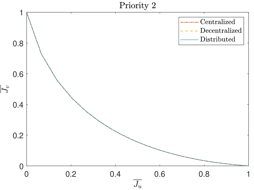
(b) Pareto-optimal front for 2nd priority.

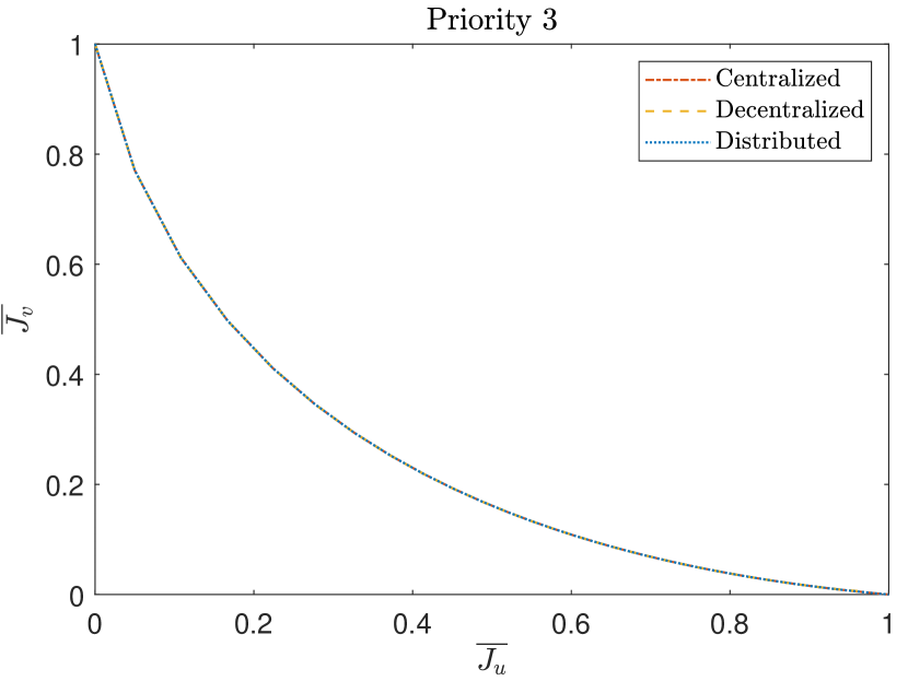
(c) Pareto-optimal front for 3rd priority.

Figure 7: Pareto-optimal fronts for three schemes (decoupled).

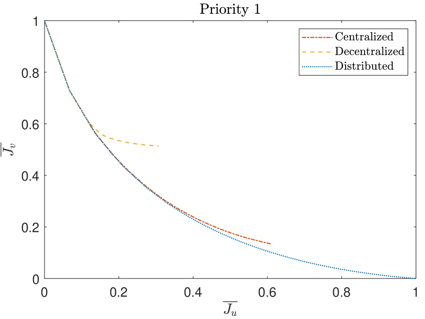
(a) Pareto-optimal front for 1st priority.

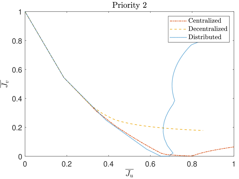
(b) Pareto-optimal front for 2nd priority.

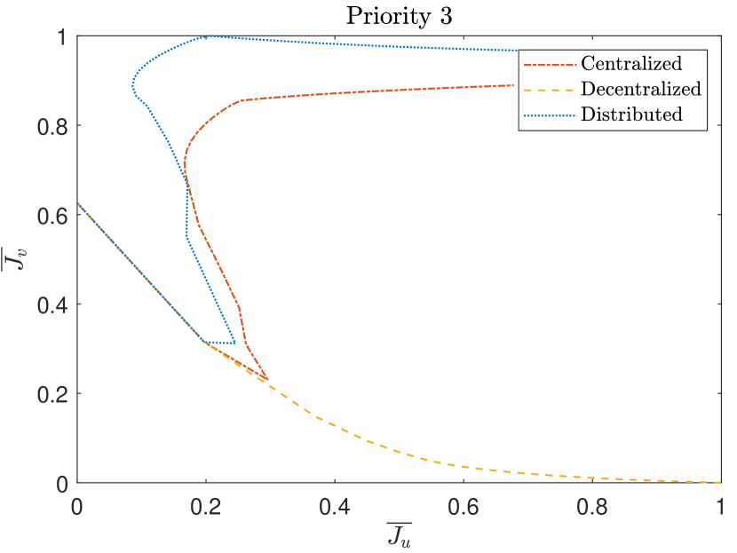
(c) Pareto-optimal front for 3rd priority.

Figure 8: Pareto-optimal fronts for three schemes (coupled, $\theta_{1}=1,\theta_{2}=0.5,\theta_{3}=0.2$).

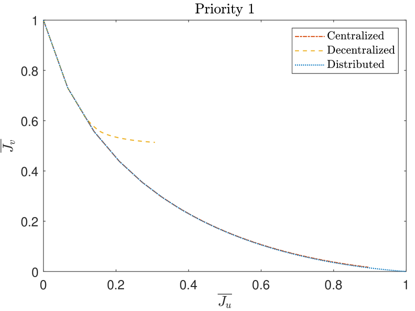
(a) Pareto-optimal front for 1st priority.

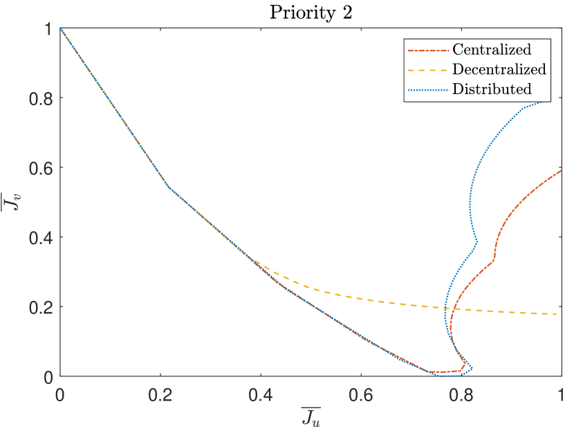
(b) Pareto-optimal front for 2nd priority.

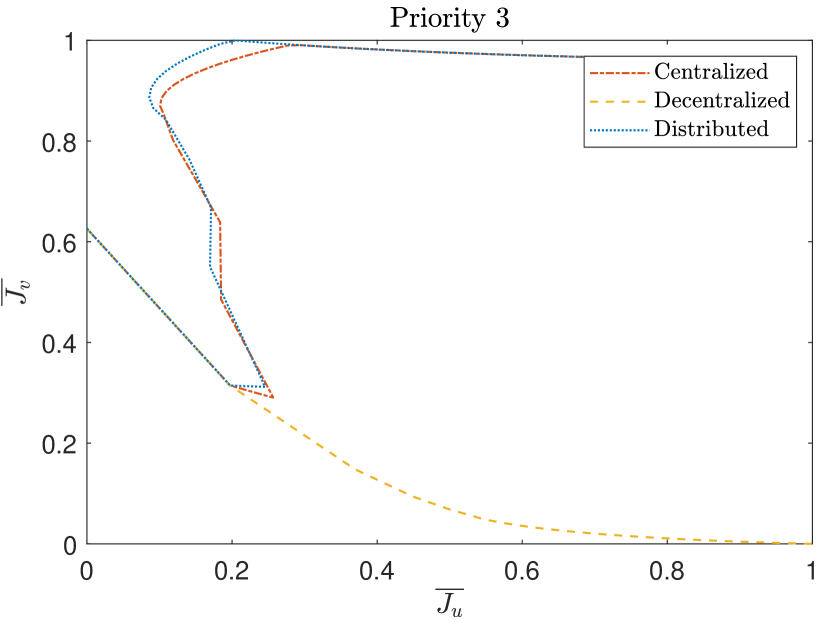
(c) Pareto-optimal front for 3rd priority.

Figure 9: Pareto-optimal fronts for three schemes (coupled, $\theta_{1}=1,\theta_{2}=0.1,\theta_{3}=0.01$).

The optimization problem (5) is actually decoupled when $\mathbf{c}^{\max}$ is taken to be a very large value, i.e. $\mathbf{c}^{\max}=[2000,2000,\cdots,2000]$, and then this energy-limited constraint is always satisfied. By changing the weight $\alpha$, Fig. 7 shows that in this case the Pareto optimal fronts of the three schemes overlap. From another point of view, if $\mathbf{c}^{\max}$ is large enough, there is practically no energy distribution problem for all the three schemes since there is always enough energy to satisfy the comfort requirements.

Modifying the energy limit $\mathbf{c}^{\max}$ to be a smaller value, i.e. $\mathbf{c}^{\max}=[2000,2000,\cdots,2000]$. There are energy couplings in subsystems because the existing energy can not satisfy the energy demand of all the rooms. The Pareto fronts are then made for simulation verification as shown in Fig. 8 ($\theta_{1}=1,\theta_{2}=0.5,\theta_{3}=0.2$) and Fig. 9 ($\theta_{1}=1,\theta_{2}=0.1,\theta_{3}=0.01$). Due to the insufficient use of information, energy is equally allocated to the subsystems in the distributed scheme, resulting in a poor optimization performance. The distributed scheme performs best for the optimization of the 1st priority subsystem, which supports Lemma 1. As the values of $\theta_{2},\theta_{3}$ decrease, the centralized Pareto front of the 2nd and 3rd priority subsystems approaches the distributed Pareto front. This is due to the mechanisms of the two schemes. The mechanism of distributed scheme is that the 2nd priority subsystem is able to use all the estimated residual energy of the 1st priority subsystem, which means that the optimization of the 2nd priority subsystem is carried out without taking into account the optimization of the subsystems with a lower priority than it, i.e., if the energy limit is very low, there is a possibility that the 2nd priority subsystem will consume all the estimated residual energy to satisfy its optimization task. The centralized mechanism uses weights to distribute the energy of each priority. Therefore, when $\theta_{2}$ is small and $\theta_{3}$ is much smaller than $\theta_{2}$, the performance of the distributed and centralized subsystems at 2nd and 3rd priority becomes close.

Table IV and Table V give the comfort index for different priority zones. The distributed scheme has the best comfort in the 1st and 2nd priorities, and the centralized scheme has the best overall comfort. There is little difference in overall comfort between the centralized and distributed solutions, both being much better than the decentralised solution.

TABLE IV: $I_{c}$ for different priority zones ($\theta_{1}=1,\theta_{2}=0.5,\theta_{3}=0.2$)

	$I_{c1}$	$I_{c2}$	$I_{c3}$	$I_{co}$
Centralized	0.1660	0.3312	0.9212	0.5021
Decentralized	0.5364	0.5364	0.4398	0.6857
Distributed	0.0007	0.0011	1.3614	0.6088

TABLE V: $I_{c}$ for different priority zones ($\theta_{1}=1,\theta_{2}=0.1,\theta_{3}=0.01$)

	$I_{c1}$	$I_{c2}$	$I_{c3}$	$I_{co}$
Centralized	0.0120	0.1132	1.2508	0.1306
Decentralized	0.5364	0.5364	0.4398	0.5643
Distributed	0.0007	0.0011	1.3614	0.1361

IV Case study

IV-A Small-scale scenario

In this scenario, a building model is built in EnergyPlus to replace the real building, which is $3.5m$ high and divided into three zones. The modeled building is shown in Fig.10, where Zone 1 takes the highest priority for energy supply, Zone 2 follows, and Zone 3 takes the lowest priority. Considering the electricity prices shown in Table III, the comfortable temperature ranges for each zone at different moments are specified as shown in Table VI.

TABLE VI: Comfortable temperature range in the small-scale scenario

Time	Zone 1	Zone 2	Zone 3
0:00-10:00	no limit	no limit	no limit
10:00-14:00	22-24∘C	22-24.5∘C	22-25∘C
14:00-17:00	22-25∘C	22-25.5∘C	22-26∘C
17:00-19:00	22-24∘C	22-24.5∘C	22-25∘C
19:00-20:00	22-25∘C	22-25.5∘C	22-26∘C
20:00-24:00	no limit	no limit	no limit

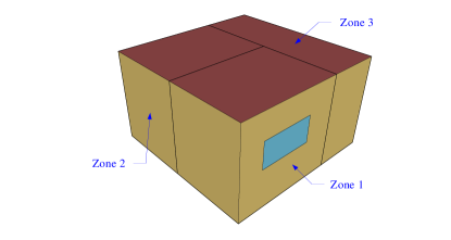
Figure 10: The building considered in the small-scale scenario.

Each zone has the same area and is equipped with an ideal variable air volume terminal device, where the supply air flow can be changed from 0 to maximum value to meet the heating or cooling load of the zone. The main parameters of the building are shown in Table VII.

TABLE VII: Major building parameters

Building parameters	Preferences
Floor area	36m2
Window to wall ratio	0.17
Occupant	1 occupant/12m2
Lighting	0.75watts/m2
Equipment	0.4watts/m2
Occupied hours	10:00am-20:00pm

IV-B Large-scale scenario

The considered large-scale scenario contains 36 zones, and the building model for the simulation experiment is shown in Fig. 11. The building has 9 floors, each of which has the same layout, and the x-th floor consists of four zones, x01, x02, x03, and x04, where x is an integer between 1 and 9. The priority classification is shown in Table VIII, and the suitable temperature interval of each zone is shown in Table IX. The computing device used for the simulation experiment is Intel(R) Xeon(R) Gold 6248R CPU @ 3.00GHz.

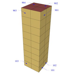
Figure 11: The building considered in the large-scale scenario.

TABLE VIII: Priority of zones

1st Priority	2nd Priority	3rd Priority
101, 102,	301, 302,
103, 104,	303, 304,	All other zones
(All zones on floor 1)	(All zones on floor 3)

TABLE IX: Comfortable temperature range in the large-scale scenario

Time	x01	x02	x03	x04
0:00-10:00	no limit	no limit	no limit	no limit
10:00-14:00	22-24∘C	22-24.5∘C	22-25∘C	22-25.5∘C
14:00-17:00	22-25∘C	22-25.5∘C	22-26∘C	22-26.5∘C
17:00-19:00	22-24∘C	22-24.5∘C	22-25∘C	22-25.5∘C
19:00-20:00	22-25∘C	22-25.5∘C	22-26∘C	22-26.5∘C
20:00-24:00	no limit	no limit	no limit	no limit

V Results

V-A Test results in the small-scale scenario

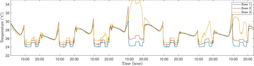
(a) Centralized strategy.

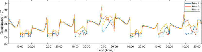
(b) Decentralized strategy.

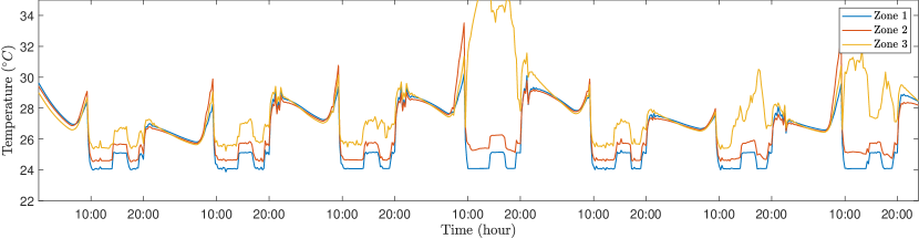
(c) Distributed strategy.

Figure 12: Indoor temperature for small-scale scenarios.

Set $\theta$ in the centralized scheme to $\theta_{1}=1,\theta_{2}=0.1,\theta_{3}=0.01$. The temperature change during the 7-day period under the centralized strategy is shown in Fig.12(a). When there is sufficient energy supply, the temperatures in all three zones meet the control requirements well. When there is insufficient energy supply, Zone 1, which has the highest priority, is met first.

The temperature change of the decentralized strategy is shown in Fig. 12(b). When the energy supply is sufficient, the decentralized strategy provides a similar control effect to that provided by the centralized strategy. When the energy supply is insufficient, the decentralized strategy is not able to distribute energy well, and thus some rooms have excess energy while others lack energy, which eventually leads to a worse control effect compared to the centralized strategy.

The temperature change curves obtained under the distributed strategy are shown in Fig. 12(c). Regardless of whether the energy supply is sufficient or not, the distributed strategy proposed in this paper ensures the comfort of the zone with the highest priority first, i.e., it can be observed that the temperature of Zone 1 (highest priority) in Fig. 12(c) is always maintained near the comfortable temperature range, and then the energy supply of other rooms is considered in the order of priority.

Fig. 13 shows the comfort index for the three strategies in the 7-day simulation. It can be seen that in both the centralized EMPC and distributed EMPC schemes, Zone 1, with the highest priority, is able to maintain a suitable temperature range, and Zone 2, with the second highest priority, is able to satisfy a certain degree of energy supply with sufficient supply from Zone 1. This shows that the performance of the proposed distributed strategy is very close to that of the centralized strategy. Fig. X shows the comfort index for different priority zones in the small-scale scenario. Our distributed scheme has the lowest $I_{co}$, which shows that our solutions make the building more comfortable at an overall level.

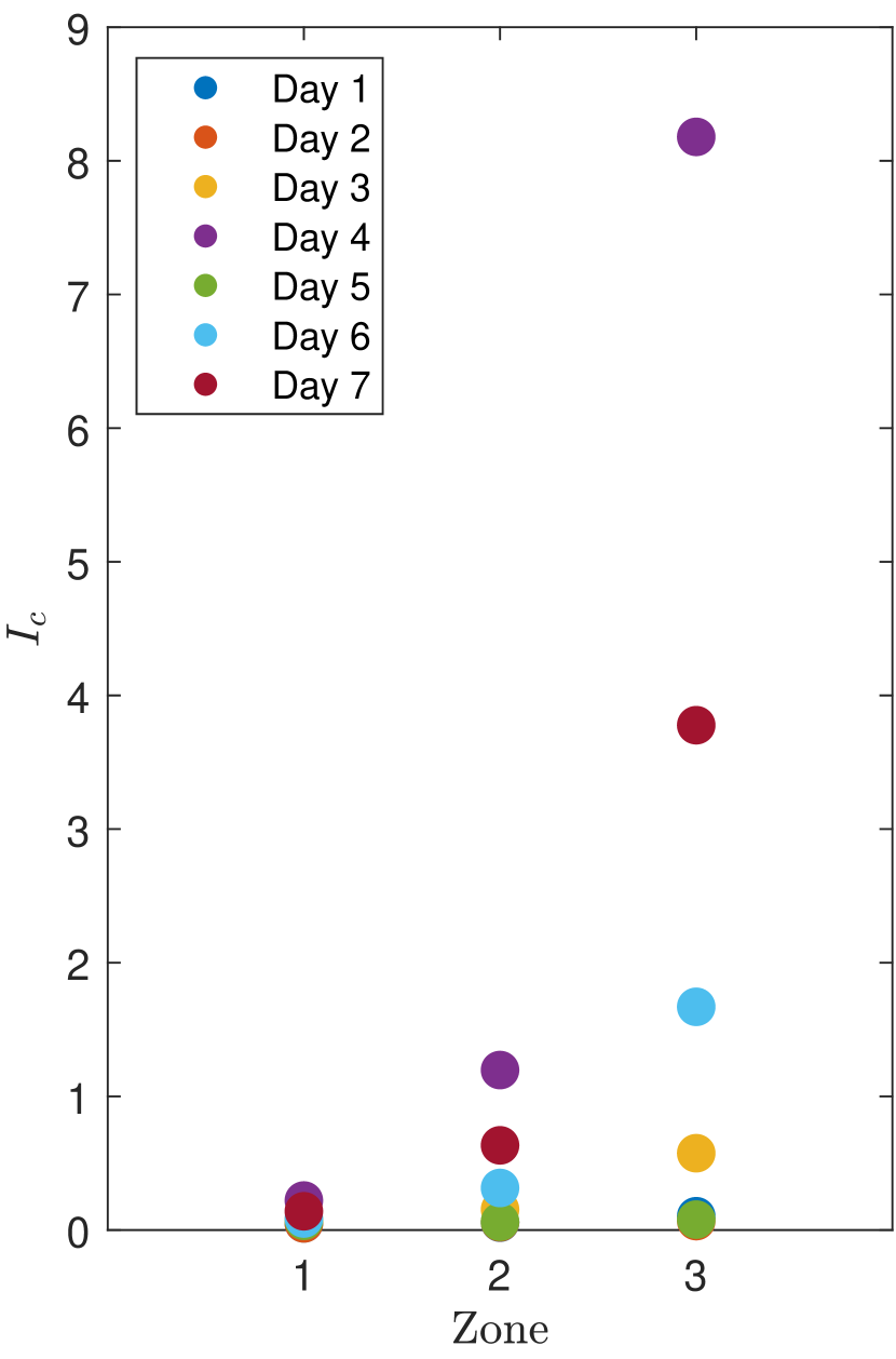
(a) Centralized strategy.

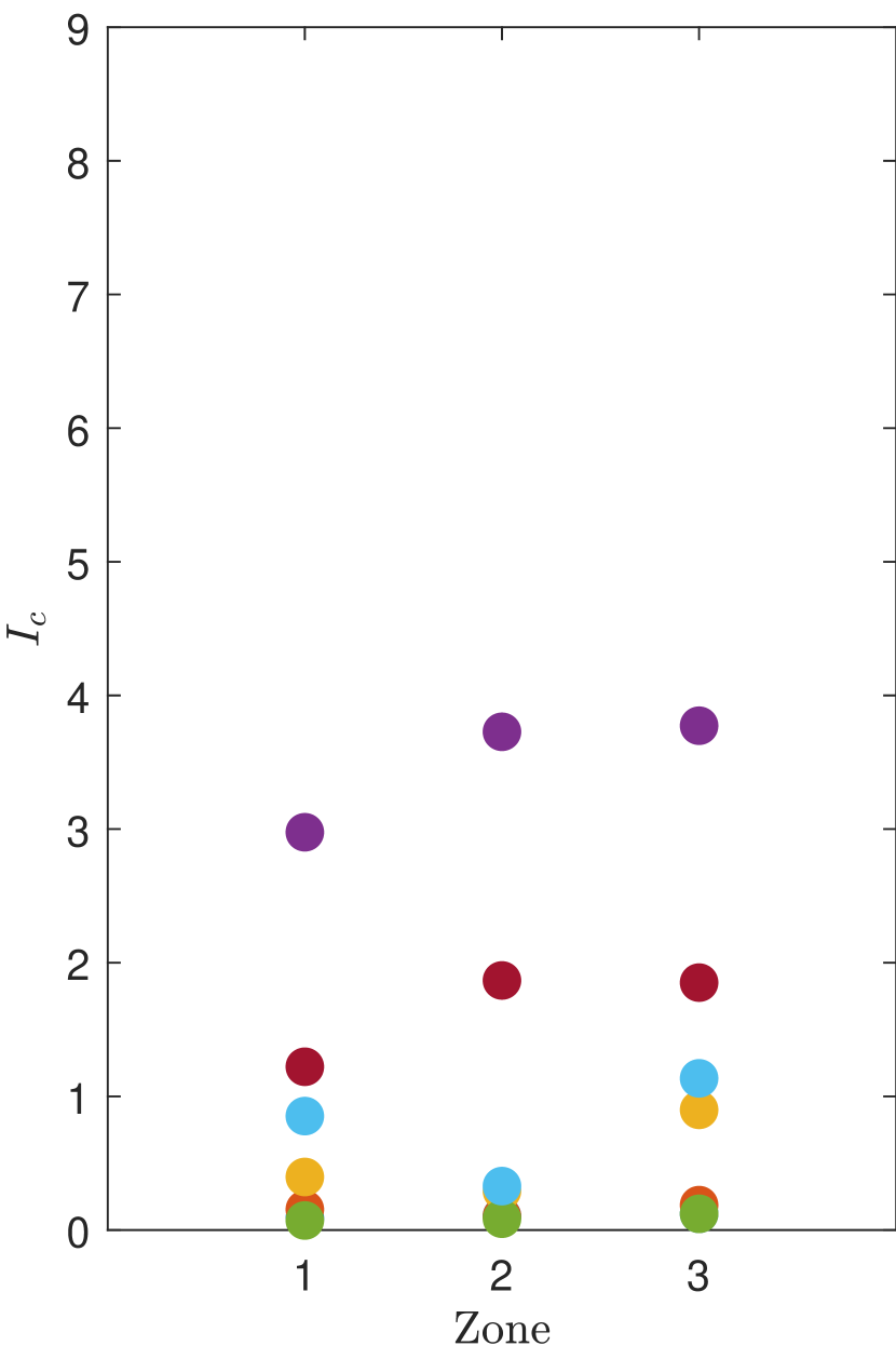
(b) Decentralized strategy.

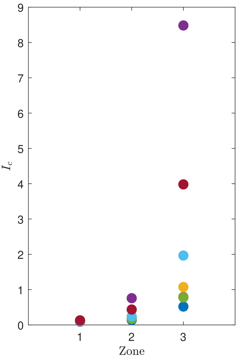
(c) Distributed strategy.

Figure 13: Comfort index for the three schemes.

TABLE X: $I_{c}$ for different priority zones in the small-scale scenario

	$I_{c1}$	$I_{c2}$	$I_{c3}$	$I_{co}$
Centralized	0.1081	0.3620	1.9402	0.2499
Decentralized	0.8230	0.9299	1.1555	0.8815
Distributed	0.1059	0.4047	2.0223	0.2617

V-B Test results in the large-scale scenario

Set $\theta$ in the centralized scheme to $\theta_{1}=1,\theta_{2}=0.1,\theta_{3}=0.01$. The temperature curves of zones with 2nd priority under centralized, decentralized and distributed EMPC strategies are shown in Fig. 14. Similar situations to that of the small-scale scenario can be observed. The centralized EMPC strategy is able to supply more sufficient energy to the zones with higher priority by adjusting the weights. The decentralized EMPC strategy has inflexible energy scheduling and is not able to satisfy the energy supply in the high priority zones. The distributed EMPC strategy has similar control performance as the centralized EMPC strategy, and it is able to satisfy the energy supply of the high priority zones even if the energy supply system does not provide enough energy for the whole system.

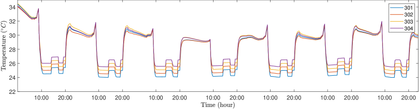
(a) Centralized strategy.

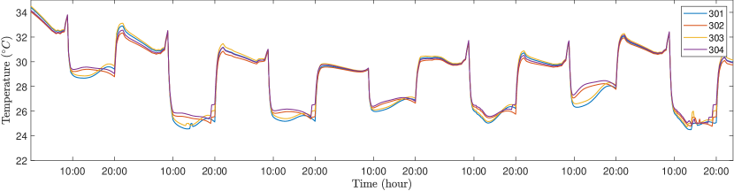
(b) Decentralized strategy.

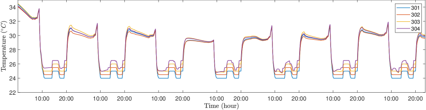
(c) Distributed strategy.

Figure 14: Indoor temperature for zones with 2nd priority (floor 3).

The comfort index for the three strategies simulated for 7 days is shown in Fig. 15. The decentralized scheme can only make the temperature comfortable in the zones with high priority when the energy supply is sufficient and cannot cope with the scenario of insufficient energy supply. Both the centralized scheme and the distributed scheme are able to make the zones with high supply priority as comfortable as possible. Fig. XI shows the comfort index for different priority zones in the large-scale scenario. Our distributed scheme has the lowest $I_{co}$, which indicates that our distribution scheme is the most reasonable.

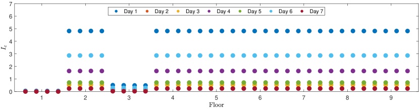
(a) Centralized strategy.

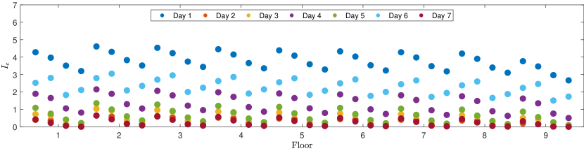
(b) Decentralized strategy.

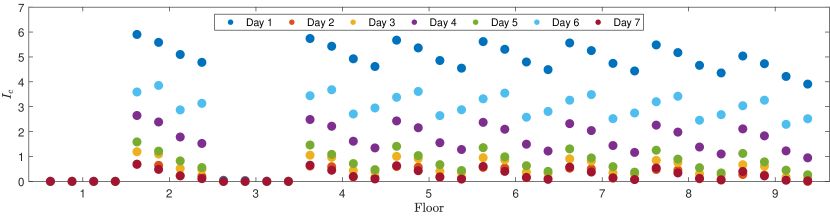
(c) Distributed strategy.

Figure 15: Comfort index for the three schemes.

TABLE XI: $I_{c}$ for different priority zones in the large-scale scenario

	$I_{c1}$	$I_{c2}$	$I_{c3}$	$I_{co}$
Centralized	0.0173	0.1613	1.5807	0.1670
Decentralized	1.2633	1.4279	1.2662	1.3476
Distributed	0.0010	0.0041	1.7107	0.1711

The computational cost of the three schemes is shown in Table XII. The size of the optimization problem to be solved by the centralized controller is related to the number of subsystems, and when the number of subsystems is relatively large, the solution is less efficient, so the computational cost of the centralized strategy is the highest among the three strategies. For a single subsystem, the size of the optimization problem to be solved is close to that of the decentralized and distributed strategies, but the computational cost of the distributed strategy is slightly higher than that of the decentralized strategy due to the exchange of information between subsystems. Since the distributed strategy performs well and the optimization problem to be solved by each subcontroller does not change as the number of subsystems increases, the distributed strategy is more suitable for scaling up to large-scale systems.

TABLE XII: Computational Cost Comparison

Centralized	Decentralized	Distributed
719.22s	313.43s	326.90s

Conclusions

In this paper, a priority-based energy distribution scheme is developed that rationally distributes energy based on priority order. For different operation scenarios, a one-to-one priority strategy and a multi-to one priority strategy based on distributed MPC are proposed. One-to-one priority strategy refers to one subsystem corresponding to one priority, and this strategy is suitable for smaller scale scenarios. Multi-to-one strategy refers to multiple subultisystems corresponding to the same priority level, and this strategy is suitable for larger scale scenarios. By exploiting the property of MPC, i.e., obtaining all the solutions in the control horizon, the subsystems can perform optimization operations in parallel.

Simulation experiments of the proposed strategy have been carried out in a 3-zone building and a 36-zone building, respectively. The experimental results show that the developed solution could satisfy the urgent energy supply in some specific zones, and the performance is close to that of the centralized scheme.

Hongyi Li received her B.S. degree in Automation and M.S. degree in Control Science and Engineering from Harbin Institute of Technology, China, in 2020 and 2023, respectively. He is currently working toward the Ph.D. degree in Control Science and Engineering from Harbin Institute of Technology, Shenzhen, China. His research interests include piecewise linear approximation and building energy conservation.

Jun Xu received her B.S. degree in Control Science and Engineering from Harbin Institute of Technology, Harbin, China, in 2005 and Ph.D. degree in Control Science and Engineering from Tsinghua University, China, in 2010. Currently, she is an associate professor in School of Mechanical Engineering and Automation, Harbin Institute of Technology, Shenzhen, China. Her research interests include piecewise linear functions and their applications in machine learning, nonlinear system identification and control.

References

- [1] D. F. Espejel-Blanco, J. A. Hoyo-Montaño, J. Arau, G. Valencia-Palomo, A. García-Barrientos, H. R. Hernández-De-León, and J. L. Camas-Anzueto, “HVAC control system using predicted mean vote index for energy savings in buildings,” Buildings, vol. 12, no. 1, p. 38, 2022.
- [2] J. Park, T. Kim, and C.-s. Lee, “Development of thermal comfort-based controller and potential reduction of the cooling energy consumption of a residential building in Kuwait,” Energies, vol. 12, no. 17, p. 3348, 2019.
- [3] Z. Sun, Z. Ma, M. Ma, W. Cai, X. Xiang, S. Zhang, M. Chen, and L. Chen, “Carbon peak and carbon neutrality in the building sector: a bibliometric review,” Buildings, vol. 12, no. 2, p. 128, 2022.
- [4] J. Too, O. A. Ejohwomu, F. K. Hui, C. Duffield, O. T. Bukoye, and D. J. Edwards, “Framework for standardising carbon neutrality in building projects,” Journal of Cleaner Production, vol. 373, p. 133858, 2022.
- [5] S. Yang, D. Yang, W. Shi, C. Deng, C. Chen, and S. Feng, “Global evaluation of carbon neutrality and peak carbon dioxide emissions: Current challenges and future outlook,” Environmental Science and Pollution Research, vol. 30, no. 34, pp. 81725–81744, 2023.
- [6] S. Ding, M. Zhang, and Y. Song, “Exploring china’s carbon emissions peak for different carbon tax scenarios,” Energy Policy, vol. 129, pp. 1245–1252, 2019.
- [7] A. Afram and F. Janabi-Sharifi, “Theory and applications of hvac control systems–a review of model predictive control (mpc),” Building and Environment, vol. 72, pp. 343–355, 2014.
- [8] J. B. Rawlings, N. R. Patel, M. J. Risbeck, C. T. Maravelias, M. J. Wenzel, and R. D. Turney, “Economic mpc and real-time decision making with application to large-scale hvac energy systems,” Computers & Chemical Engineering, vol. 114, pp. 89–98, 2018.
- [9] S. Gupta, P. Bansal, R. Gupta, and M. Mewara, “Optimal tuning of pid controller parameters for hvac system using bf-pso algorithm,” in 2023 IEEE 4th Annual Flagship India Council International Subsections Conference (INDISCON), pp. 1–5, IEEE, 2023.
- [10] E. Saloux and J. A. Candanedo, “Optimal rule-based control for the management of thermal energy storage in a canadian solar district heating system,” Solar Energy, vol. 207, pp. 1191–1201, 2020.
- [11] B. Alimohammadisagvand, J. Jokisalo, and K. Sirén, “Comparison of four rule-based demand response control algorithms in an electrically and heat pump-heated residential building,” Applied Energy, vol. 209, pp. 167–179, 2018.
- [12] R. Eini and S. Abdelwahed, “Distributed model predictive control for intelligent traffic system,” in 2019 International Conference on Internet of Things (iThings) and IEEE Green Computing and Communications (GreenCom) and IEEE Cyber, Physical and Social Computing (CPSCom) and IEEE Smart Data (SmartData), pp. 909–915, IEEE, 2019.
- [13] A. J. del Real, A. Arce, and C. Bordons, “Combined environmental and economic dispatch of smart grids using distributed model predictive control,” International Journal of Electrical Power & Energy Systems, vol. 54, pp. 65–76, 2014.
- [14] Y. Zhang, Y. Zheng, and S. Li, “Enhancing cooperative distributed model predictive control for the water distribution networks pressure optimization,” Journal of Process Control, vol. 84, pp. 70–88, 2019.
- [15] D. Fu, H.-T. Zhang, A. Dutta, and G. Chen, “A cooperative distributed model predictive control approach to supply chain management,” IEEE Transactions on Systems, Man, and Cybernetics: Systems, vol. 50, no. 12, pp. 4894–4904, 2019.
- [16] L. Chen, H. Hopman, and R. R. Negenborn, “Distributed model predictive control for cooperative floating object transport with multi-vessel systems,” Ocean Engineering, vol. 191, p. 106515, 2019.
- [17] Z. Cai, H. Zhou, J. Zhao, K. Wu, and Y. Wang, “Formation control of multiple unmanned aerial vehicles by event-triggered distributed model predictive control,” IEEE Access, vol. 6, pp. 55614–55627, 2018.
- [18] A. Bono, G. Fedele, and G. Franzè, “A swarm-based distributed model predictive control scheme for autonomous vehicle formations in uncertain environments,” IEEE Transactions on Cybernetics, vol. 52, no. 9, pp. 8876–8886, 2021.
- [19] N. Lefebure, M. Khosravi, M. H. Badyn, F. Bünning, J. Lygeros, C. Jones, and R. S. Smith, “Distributed model predictive control of buildings and energy hubs,” Energy and Buildings, vol. 259, p. 111806, 2022.
- [20] P.-D. Moroşan, R. Bourdais, D. Dumur, and J. Buisson, “A distributed mpc strategy based on benders’ decomposition applied to multi-source multi-zone temperature regulation,” Journal of Process Control, vol. 21, no. 5, pp. 729–737, 2011.
- [21] R. E. Jalal and B. P. Rasmussen, “Limited-communication distributed model predictive control for coupled and constrained subsystems,” IEEE Transactions on Control Systems Technology, vol. 25, no. 5, pp. 1807–1815, 2016.
- [22] C. J. Bay, R. Chintala, V. Chinde, and J. King, “Distributed model predictive control for coordinated, grid-interactive buildings,” Applied Energy, vol. 312, p. 118612, 2022.
- [23] M. Mork, A. Xhonneux, and D. Müller, “Nonlinear distributed model predictive control for multi-zone building energy systems,” Energy and Buildings, vol. 264, p. 112066, 2022.
- [24] J. Zhao, “Energyplus model-based predictive control (epmpc) by using matlab/simulink and mle+,” 2013.
- [25] D. B. Crawley, L. K. Lawrie, F. C. Winkelmann, W. F. Buhl, Y. J. Huang, C. O. Pedersen, R. K. Strand, R. J. Liesen, D. E. Fisher, M. J. Witte, et al., “Energyplus: creating a new-generation building energy simulation program,” Energy and buildings, vol. 33, no. 4, pp. 319–331, 2001.
- [26] H. Li, J. Xu, Q. Zhao, and S. Wang, “Economic model predictive control in buildings based on piecewise linear approximation of predicted mean vote index,” IEEE Transactions on Automation Science and Engineering, 2023.