LaCE-LHMP: Airflow Modelling-Inspired Long-Term Human Motion Prediction By Enhancing Laminar Characteristics in Human Flow

Abstract

Long-term human motion prediction (LHMP) is essential for safely operating autonomous robots and vehicles in populated environments. It is fundamental for various applications, including motion planning, tracking, human-robot interaction and safety monitoring. However, accurate prediction of human trajectories is challenging due to complex factors, including, for example, social norms and environmental conditions. The influence of such factors can be captured through Maps of Dynamics (MoDs), which encode spatial motion patterns learned from (possibly scattered and partial) past observations of motion in the environment and which can be used for data-efficient, interpretable motion prediction (MoD-LHMP). To address the limitations of prior work, especially regarding accuracy and sensitivity to anomalies in long-term prediction, we propose the Laminar Component Enhanced LHMP approach (LaCE-LHMP). Our approach is inspired by data-driven airflow modelling, which estimates laminar and turbulent flow components and uses predominantly the laminar components to make flow predictions. Based on the hypothesis that human trajectory patterns also manifest laminar flow (that represents predictable motion) and turbulent flow components (that reflect more unpredictable and arbitrary motion), LaCE-LHMP extracts the laminar patterns in human dynamics and uses them for human motion prediction. We demonstrate the superior prediction performance of LaCE-LHMP through benchmark comparisons with state-of-the-art LHMP methods, offering an unconventional perspective and a more intuitive understanding of human movement patterns.

I INTRODUCTION

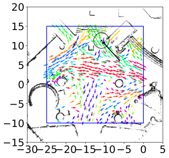
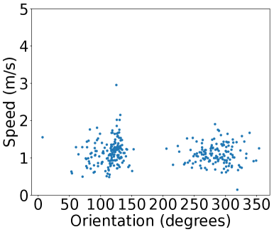
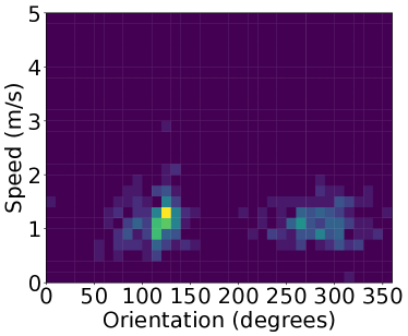
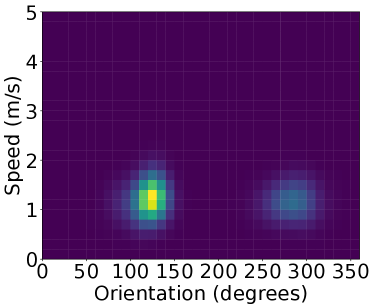
Figure 1: Example of laminar component extraction in LaCE-LHMP. Upper-left: LaCE model of a location in a shopping mall. Colored arrows show flow directions with highest likelihoods; Upper-right: raw data (velocity observations) in the $\omega-\nu$ domain (i.e. speed and orientation) at a specific location; Lower-left: histogram of the raw data $\Gamma^{R}$; Lower-right: extracted laminar component $\Gamma^{L}$. The laminar component is used for motion prediction in LaCE-LHMP.

Long-term human motion prediction (LHMP) plays an important role in ensuring the safe operation of autonomous robots and vehicles in populated environments [1]. Accurate prediction of people’s future trajectories over a prolonged duration stands as a fundamental requirement for various applications, including optimized motion planning, refined tracking, advanced automated driving, improved human-robot interaction, and enhanced intelligent safety monitoring and surveillance. Accurate LHMP not only improves operational efficiency in relevant applications but also fosters a higher level of acceptance among users and stakeholders, as they can trust the systems to understand and anticipate human motion more reliably.

Human motion is complex, influenced by various factors, including not only an individual’s intrinsic intent and dynamics but also external influences such as social conventions and environmental cues. These factors collectively contribute to the challenge of accurately predicting human motion [1]. Especially for predictions over an extended, very long time horizon (20 seconds and more), the impact of complex, large-scale environments on human behavior needs to be accounted for. Unlike for short-term predictions, where considering only the current state and immediate interactions can suffice, the long-term perspective demands explicit modelling of how the environment continuously shapes and directs human motion. These influences cannot be adequately summarized just by the current state of the individual and observed interactions but instead require explicit modelling [2].

An effective approach to address this challenge is to use maps of dynamics (MoDs). MoDs [3] are maps that encode spatial or spatio-temporal motion patterns as a feature of the environment. MoD-informed long-term human motion prediction (MoD-LHMP) approaches are particularly suited to predict motion in the long-term perspective, where the environment effects become critical for making accurate predictions. By using MoDs, motion prediction can utilize previously observed spatial motion patterns that encode important information about spatial motion patterns in a given environment. Among the MoD-LHMP methods, Zhu et al. [4] utilize CLiFF-maps [5], which capture multimodal statistical information about human flow patterns, to make long term predictions. CLiFF-LHMP is shown to make accurate long-term predictions, even when trained with small amounts of data [6]. However, the modelling approach based on the CLiFF map may struggle to differentiate dominant human flow from irregular motion, and therefore the prediction accuracy may be affected by anomalous data.

Detecting and identifying abnormal trajectories is a major challenge in motion modelling and prediction. Existing methods typically identify abnormal motions by comparing them to expected behaviors [7] or measuring deviations from normal motions [8]. However, these approaches require labelled data for supervised learning.

In this paper, we propose the Laminar Component Enhanced (LaCE) LHMP approach inspired by data-driven airflow modelling [9]. Airflow can be characterized as a combination of laminar and turbulent flow patterns in fluid dynamics [10, 11]. Similarly, we postulate that human trajectory patterns share this property, with laminar components representing predictable motion and turbulent flow components reflecting more unpredictable and arbitrary motion. Accordingly, the proposed LaCE-LHMP approach extracts laminar patterns in human dynamics and uses them for motion prediction, mitigating the impact of anomalous data in an unsupervised manner. During the prediction process, the degree of laminar dominance is quantitatively measured to make adaptive adjustments to the contribution of the laminar component. LaCE-LHMP also ranks the predicted trajectories and provides the most likely output, offering practical utility for autonomous robots. Our approach shares the benefits of the prior art in MoD-LHMP, while addressing its limitations.

We demonstrate the proposed approach in quantitative and qualitative experiments, comparing it to several state-of-the-art LHMP methods. The superior prediction accuracy is promising and supports the hypothesis that human motion in real-world environments comprises underlying laminar patterns. We note that the LaCE-LHMP approach not only improves prediction performance but also offers an unconventional perspective on motion prediction and allows for a more intuitive understanding of human movement patterns. Furthermore, our approach can detect regions with more prominent laminar patterns, which are more predictable than those with predominantly turbulent patterns. The extent of laminar dominance within an environment can be used for robot motion planning and exploration tasks.

II RELATED WORK

The numerous works in trajectory prediction attempt to consider various factors that influence human motion, such as observed dynamics, elements of the static environment, semantic features and social interactions. Based on the underlying principle for the motion model, they can be categorized into pattern-, physics- and planning-based approaches [1].

Pattern-based approaches rely on learning patterns and regularities from historical motion data. They use techniques such as Hidden Markov Models, Gaussian Processes and in particular neural networks, to capture temporal dependencies and probabilistic relationships in trajectory data. Recurrent Neural Network (RNN) approaches [12, 13, 14, 1] model temporal dynamics and capture non-linear temporal dependencies, while the approaches based on CNNs (Convolutional Neural Networks) extract spatial features that are relevant for motion dynamics [15, 16, 17, 18]. Generative models like GANs (Generative Adversarial Network) [19, 20], and CVAEs (Conditional Variational Autoencoder) [21, 22, 23] capture dynamic, non-linear dependencies under epistemic uncertainty. Transformer-based architectures introduce attention mechanisms for context understanding [24]. Many of these approaches primarily focus on predicting stochastic interactions between diverse moving agents in the short-term perspective in scenarios where the effect of the environment topology and semantics is minimal.

Physics-based approaches construct kinematic models that focus primarily on intrinsic motion dynamics. One such simple yet effective approach is the Constant Velocity Model (CVM), which has demonstrated competitive predictive potential in the short term [25]. However, CVM falls short when applied to long-term prediction tasks, as it lacks the environmental information, external social interactions and cognitive factors. Other examples of physics-based methods include the Social Force model [26, 27, 28], Reciprocal Velocity Obstacles approaches [29] and their extensions such as ORCA [30], methods based on dynamics such as Switching Linear Dynamical Systems (SLDS) [31]. These approaches perform well in certain situations, e.g. for short-term modelling of vehicle dynamics, but, similarly to the CVM, struggle in the long-term perspective.

Planning-based methods, for instance using Markov Decision Processes, have shown a clear potential in the long-term [32, 33, 34]. Using the map as input, these methods are able to produce long-term non-linear paths towards to distant goals. Still, these methods make optimality assumptions of human motion, which may not always hold in practice. Some further approaches are designed to predict trajectories over extensive durations requiring, however, auxiliary inputs like RGB images [35, 36] to make predictions.

In contrast, our model, LaCE-LHMP, works without explicit knowledge of the environment, and does not require further inputs apart from the observed motion sequence. Instead, it implicitly infers environmental factors and common goals from a representation of observed spatial motion patterns, encoded in the Map of Dynamics (MoD), similarly to CLiFF-LHMP [6, 4]. It combines aspects of physics-based and pattern-based approaches, namely the velocity-based transition model and generalization of observed motion. Differently from the prior art, LaCE-LHMP makes the assumption that human motion can be described with laminar-turbulence characteristics similar to airflow and, accordingly, extracts the laminar human motion component to predict motion more accurately.

III METHOD

III-A Problem statement

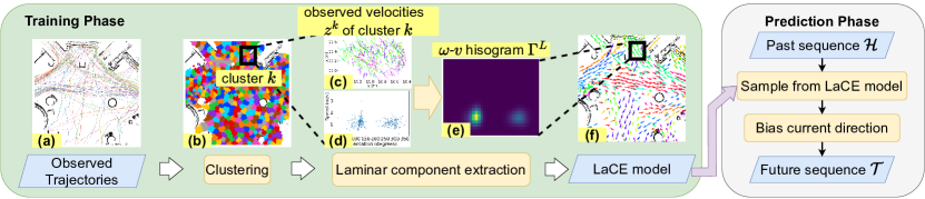
Figure 2: Diagram illustrating the training and prediction phases of the LaCE-LHMP approach. In the training phase, observed trajectories (a) are used. Velocity observations, which are depicted in (c) for $(x,y)$ and (d) for $\omega$-$\nu$ distribution, are clustered using K-means into K clusters, shown in (b). From each cluster’s joint $\omega$-$\nu$ distribution, a discrete $\omega$-$\nu$ histogram $\Gamma^{R}$ is estimated to extract the laminar component $\Gamma^{L}$, as shown in (e). The directions with the highest likelihood in $\Gamma^{L}$ are represented by colored arrows in the LaCE model (f). The LaCE model is then utilized for prediction.

We frame the task of predicting a person’s future trajectory as inferring a sequence of future states. With the input of an observation history of $O_{p}$ past states of a person, the method predicts $T_{p}$ future states. The length of the observation history is $O_{s}\in\mathbb{R}^{+}$ $\text{\,}\mathrm{s}$. With the current time-step denoted as the integer $t_{0}\geq 0$, the sequence of observed states is $\mathcal{H}=\langle s_{t_{0}-1},...,s_{t_{0}-O_{p}}\rangle$, where $s_{t}$ is the state of a person at time-step $t$. A state is represented by 2D Cartesian coordinates $(x,y)$, direction $\omega$, and speed $\nu$: $s=(x,y,\omega,\nu)$. From the observed sequence $\mathcal{H}$, we derive the observed speed $\nu_{\mathrm{obs}}$ and direction $\omega_{\mathrm{obs}}$ at time-step $t_{0}$. Then the current state becomes $s_{t_{0}}=(x_{t_{0}},y_{t_{0}},\omega_{\mathrm{obs}},\nu_{\mathrm{obs}})$.

Given the current state $s_{t_{0}}$, we estimate a sequence of future states. Similar to past states, future states are predicted within a time horizon $T_{s}\in\mathbb{R}^{+}$ $\text{\,}\mathrm{s}$. $T_{s}$ is equivalent to $T_{p}~{}\geq~{}1$ prediction time steps, assuming a constant time interval $\Delta t$ between two predictions. Thus, the prediction horizon is $T_{s}=T_{p}\Delta t$. The predicted sequence is then denoted as $\mathcal{T}=\langle s_{t_{0}+1},s_{t_{0}+2},...,s_{t_{0}+T_{p}}\rangle$.

III-B Overview of the LaCE-LHMP approach

The LaCE-LHMP approach consists of training and prediction phases, as shown in LABEL:{fig:master_figure}. The training phase first extracts the underlying laminar component from the observed trajectories (described in Sec. III-C) and learns an MoD, expressed through a set of probabilistic representations of the target area, i.e., the LaCE model. In the prediction phase, both the observed recent trajectory sequence and the learned LaCE model influence the predicted trajectory, depending on the degree of local laminar dominance. In order to select the contributions from both factors depending on the local situation, we propose an adaptive sampling process, see Sec. III-D. Once a likely direction is sampled, the current state can be propagated to predict sequences of future states.

III-C Laminar component extraction for enhancing LHMP

The process of extracting laminar components from observed human trajectories involves three sequential steps:

1. Spatial clustering: We apply K-means clustering to group velocity observations within the area of interest into $K$ clusters, by spatial coordinates $(x,y)$ for calculating pairwise distances, as shown in Fig. 2(b). Since the trajectories are not uniformly distributed in the target area, clustering them allows to learn more accurate, representative location-specific flow distributions in both densely and sparsely observed regions.

2. Local $\omega$-$\nu$ distribution modelling: Under the assumption that clusters and the respective joint distributions of directions ($\omega$) and speeds ($\nu$) are sufficiently stable over time, we estimate a discrete $\omega$-$\nu$ histogram $\Gamma^{R}$ to represent each cluster’s joint $\omega$-$\nu$ distribution from the observed velocities $z^{k}_{i}=(\omega,\nu),i=1,2,3,\dots,N^{k}$, belonging to cluster $k$, shown in Fig. 2(d). $\Gamma^{R}$ consists of $N_{S}$ discrete states, each encapsulating unique combinations of direction and speed. State $J$ represents the estimated probability of a velocity possessing $(\omega_{J},\nu_{J}$). Given $N^{k}$ observations in the cluster, $\Gamma^{R}$ is given by

   $$\Gamma^{R}(J|\mathbf{z}_{1:N^{k}})=\frac{f_{J,N^{k}}}{\sum_{j=1}^{N_{S}}f_{J_{j},N^{k}}}$$ (1)

   where $f_{J_{j},N^{k}}$ is the observed frequency of the $j$-th state at the cluster $k$.

3. Laminar component extraction: $\Gamma^{R}$ gives an intuitive sense of the underlying $\omega$-$\nu$ distribution. In reality, $\Gamma^{R}$ is typically a mixture of more predictable laminar components and “chaotic”, turbulent components. Extracting $\Gamma^{R}$’s laminar component aids unseen trajectory prediction because it is reasonable to assume that its current $(\omega,\nu)$ depends on its recent $(\omega,\nu)$ as well as the underlying laminar pattern. As shown in Fig. 2(e), $\Gamma^{L}(J|\mathbf{z}_{1:t})$ denotes the laminar component of $\Gamma^{R}$. $\Gamma^{L}(J|\mathbf{z}_{1:t})$ is estimated using a Bayes filter [37], as shown in Alg. 1, originally from [9].

   Data: Number of states, $N_{S}$

   Total number of observations in the considered cluster $k$, $N^{k}$

   The $i$-th observation, $z_{1},z_{2},z_{i},\ldots,z_{N^{k}}$

   Result: Laminar component $\Gamma^{L}(J|\mathbf{z}_{1:N^{k}})$ for each $J$

   1 Initialization:

   2 Initialize the prior of ${p}_{J,i}$ without any observation as ${p}_{J,i=0}=1/{N_{S}}$ for each $J$

   3

   4for $i\leftarrow 1$ to $N^{k}$ do

   5       Calculate $\bar{p}(J,i)$ using the $p(J,i)$ and $\mathcal{C}(J|J_{j},\mathbf{z}_{1:i})$, given by

   $$\bar{p}_{J,i}=\sum_{j=1}^{N_{S}}{p}_{J_{j},i-1}\mathcal{C}(J|J_{j},\mathbf{z}_{1:i})$$

   where $\mathcal{C}(J|J_{j},\mathbf{z}_{1:i})$ is a transition model that accounts for the variability of $(\omega,\nu)$ (see Eq.3);

   6      

   7      Calculate $p_{J,i}$ using

   $$p_{J,i}=\frac{\bar{p}_{J,t}\mathcal{M}(z_{i}|J)}{\sum^{N_{S}}_{j=1}\bar{p}_{J_{j},i}\mathcal{M}(z_{i}|J_{j})}$$

   where $\mathcal{M}(z_{i}|J_{j})$ is a measurement model defined by Eq. 2;

   8      

   9      Calculate $\Gamma^{L}(J|\mathbf{z}_{1:i})$ using

   $$\Gamma^{L}(J|\mathbf{z}_{1:i})=\frac{\Gamma^{L}(J|\mathbf{z}_{1:i-1})+p_{J,i}}{\sum_{j=1}^{N_{S}}\Gamma^{L}(J_{j}|\mathbf{z}_{1:i})}$$

   .

   10      

   11 end for

   12

   Output: $\Gamma^{L}(J|\mathbf{z}_{1:N^{k}})$ for each $J$ given all $N^{k}$ observations

   13

   Algorithm 1 Bayes Filter to extract laminar components

The Bayes filter plays a critical role in Alg. 1 for updating the likelihood for each state $J$. The Bayes filter incorporates the empirical knowledge of the uncertainty with an observed $z=(\omega,\nu)$ using a measurement model given by

$$\mathcal{M}(z|J)=\frac{1}{2\pi\sigma_{\omega}\sigma_{\nu}}\mathbf{exp}-\Bigg{(}\frac{\Delta(\omega,J_{\omega})^{2}}{2\sigma_{\omega}^{2}}+\frac{|\nu-J_{\nu}|^{2}}{2\sigma_{\nu}^{2}}\Bigg{)}$$ (2)

where $\Delta(\omega,J_{\omega})$ and $|\nu-J_{\nu}|$ correspond to great-circle distance and spatial distance (e.g., Euclidean distance) between measurement $z=(\omega,\nu)$ and the state $J(J_{\omega},J_{\nu})$, respectively. Parameters $\sigma_{\omega}$ and $\sigma_{\nu}$ correspond to the confidence intervals with respect to the variables of direction variable and speed, which can be set empirically. The measurement model is used in the transition model given by Eq. 3:

$$\mathcal{C}(J|J_{j},\mathbf{z}_{1:i})=\mathcal{C}(J|J_{j},z_{1:i-1})+\mathcal{M}(z_{i}|J)$$ (3)

which assigns a posterior to each state $J$ based on the frequency of the transition between $J$ and another state $J_{j}$. This transition model enables the suppression of the posteriors of states associated with intermittent transitions, thereby enhancing the discernibility of laminar dominant states. A comparison of the visualized raw trajectory data, the corresponding probabilistic representation $\Gamma^{R}$, and the extracted laminar component $\Gamma^{L}$ is provided in Fig. 1.

III-D Adaptive sampling based on Laminar-dominant condition

Considering that both the observed part of the trajectory and the underlying laminar pattern can contribute to the prediction, the our method involves a trade-off between relying on the laminar component or adapting to recent observations. For this reason, it is useful to quantify the degree of laminar dominance to guide the trade-off. In our proposed approach, the Kullback-Leibler (KL) divergence between $\Gamma^{R}$ and $\Gamma^{L}$, denoted as $D_{KL}(\Gamma^{R}\parallel\Gamma^{L})$, serves as an indicator of thelaminar dominance. A larger divergence value corresponds to a lower degree of laminar dominance.

In the prediction phase, to estimate $\mathcal{T}$, for each prediction time step, we sample a direction from the laminar component corresponding to the current position. Assuming that a person tends to continue walking at the same speed as in the last time step, we bias the direction of motion with the direction $\omega_{s}$ sampled from $\Gamma^{L}$, as $\omega_{t}=\omega_{t-1}+(\omega_{s}-\omega_{t-1})\cdot K(\omega_{s}-\omega_{t-1})$, where $K(\cdot)$ is a kernel function that defines the degree of impact of the sampled direction. To define the degree of laminar dominance, we employ a Gaussian kernel with the KL divergence serving as the kernel width, $K(x)=e^{-\beta\left\|x\right\|^{2}}$, where $\beta=10^{D_{KL}(\Gamma^{R}\parallel\Gamma^{L})}$. When there is high divergence, indicating low laminar dominance at the current location, the proposed method tends to behave more like a CVM. Conversely, with smaller divergence, suggesting the position is likely to be laminar dominated, and therefore, the prediction will align more with a laminar pattern.

IV EXPERIMENTS

This section describes the experimental setup for qualitative and quantitative evaluation of the proposed approach.

Dataset: For evaluation, we use the ATC shopping mall dataset [38]. This dataset covers a large indoor environment with a total area of around $900\text{\,}{\mathrm{m}}^{2}$. Given the immense length of the ATC dataset (92 days), we use a subset of 10 days in the experiments, with the first day for training and the remaining 9 days for evaluation. For both our methods and baselines, we use the same training and evaluation data.

Baselines: We compare the performance of our approach with three baselines: CLiFF-LHMP, Trajectron++ and CVM.

CLiFF-LHMP [4], similarly to LaCE-LHMP, is based on Maps of Dynamics, but uses a different representation of human motion, namely the CLiFF-map. Differently from LaCE-LHMP, the CLiFF-map has a regular grid structure and uses Gaussian Mixture Modelling to detect the dominant motion patterns in each grid cell. Importantly, it does not factor our the turbulent component of the training data. Previously, the CLiFF approach was validated with the ATC dataset [38] compared to a vanilla LSTM model as a baseline [6]. The results show that the CLiFF approach outperforms the LSTM model at the long prediction horizons of up to 60 seconds in terms of the average and final displacement errors. The superior performance of CLiFF-LHMP makes it a suitable baseline algorithm for our comparative study.

Trajectron++ (T++) [21] represents a state-of-the-art approach employing a graph-structured generative neural network based on a conditional-variational autoencoder. To run T++ we used public code and trained the model for 100 epochs on the training day of ATC dataset. Parameter configurations are provided with project code.

Implementation details: Given the map of the ATC environment, we focus on the central square area highlighted by the blue square in Fig. 3. This area has dimensions where $X$ ranges from $-$25 to 0 and $Y$ ranges from $-$10 to 15, amounting to an area of $625\text{\,}{\mathrm{m}}^{2}$. In contrast to the east corridor, the central square offers a more open space, allowing pedestrians greater freedom of movement and presenting more obstacles. Conversely, the human flow patterns in the east corridor are simpler and more restricted.

In the experiments, the ATC dataset was downsampled to 1 Hz. We use an observation horizon of $3\text{\,}\mathrm{s}$ for input and the following trajectory (up to $20\text{\,}\mathrm{s}$ long) as the ground truth.

For parameter settings of all the methods, prediction horizon $T_{s}$ is set to 1–20 $\mathrm{s}$, and observation horizon $O_{s}$ is $3\text{\,}\mathrm{s}$. Prediction time step $\Delta t$ is set to $1\text{\,}\mathrm{s}$. In the experiment, the values of $\omega_{\mathrm{obs}}$ and $\nu_{\mathrm{obs}}$ are calculated as a weighted sum of the finite differences in the observed state, as in the recent ATLAS benchmark [39]. With the same parameters as in [39], the sequence of observed velocities is weighted with a zero-mean Gaussian kernel with $\sigma=1.5$ to put more weight on more recent observations, such that $\omega_{\mathrm{obs}}=\sum_{t=1}^{O_{p}}\omega_{t_{0}-t}g(t)$ and $\nu_{\mathrm{obs}}=\sum_{t=1}^{O_{p}}v_{t_{0}-t}g(t)$, where $g(t)=(\sigma\sqrt{2\pi}e^{\frac{1}{2}(\frac{t}{\sigma})^{2}})^{-1}$. For the LaCE-LHMP experiment, in the spatial clustering step, cluster number $K$ is set to 500, targeting each cluster region to cover approximately $1\text{\,}{\mathrm{m}}^{2}$ . In constructing the discrete $\omega$-$\nu$ histogram, speed ($\nu$) bins are defined at $0.2\text{\,}\mathrm{m}\text{\,}{\mathrm{s}}^{-1}$ intervals, ranging from 0 to $5\text{\,}\mathrm{m}\text{\,}{\mathrm{s}}^{-1}$, and direction ($\omega$) bins are defined at 10-degree intervals, covering the full 360-degree range.

Evaluation metrics: For the evaluation of the predictive performance, we used the following metrics: Average and Final Displacement Errors (ADE and FDE) and Top-k ADE/FDE. ADE describes the mean $L^{2}$ distance between predicted trajectories and the ground truth. FDE describes the $L^{2}$ distance between the predicted final position and the ground truth final position at the last prediction time step. Top-k ADE/FDE compute the displacements between the ground truth position and the closest of the $k$ predicted trajectories. $k$ is set to 5 in the evaluation.

For evaluating T++, we use the most-likely output configuration, which generates deterministic and most-likely single output. When evaluating our approach, for any given observed sequence, LaCE-LHMP can be executed multiple times to randomly generate a set of predicted trajectories. Based on practical applications for autonomous robots, LaCE-LHMP can rank these predicted trajectories and provide the most likely output. The probability of the output sequence $\mathcal{T}$ is calculated as the product of probabilities of samples taken from histograms over $\mathcal{T}_{p}$ prediction time steps. A higher probability results in a higher ranking. For CLiFF-LHMP, we determine the likelihood of the sampled velocity using the probability density function of the Semi-Wrapped Gaussian Mixture Model distribution. For robustness evaluation, both CLiFF-LHMP and LaCE-LHMP are run 10 times and standard deviations are shown in Table I.

V RESULTS

Method	ADE / FDE	Top-k ADE / FDE
CVM	4.26 / 9.01	-
Trajectron++	6.09 / 12.86	2.96 / 5.86
CLiFF-LHMP	3.52$\pm$0.009 / 7.40$\pm$0.021	3.00 / 6.09
LaCE-LHMP (Ours)	3.31$\pm$0.006 / 6.93$\pm$0.013	3.00 / 6.13

TABLE I: Long-term prediction ($20\text{\,}\mathrm{s}$) results on the ATC dataset. With $O_{s}=$3\text{\,}\mathrm{s}$$, errors are reported as ADE/FDE in meters.

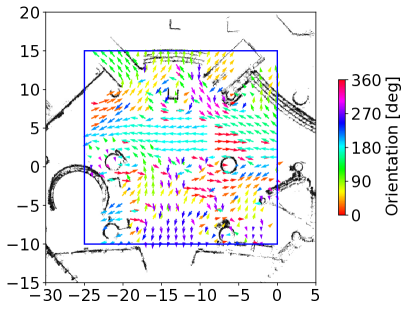
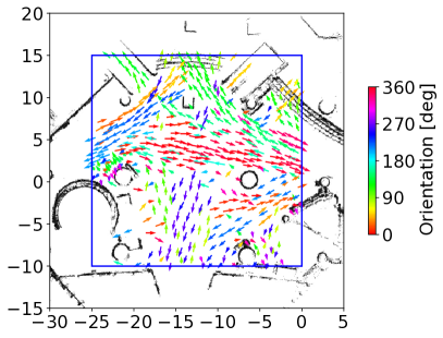
Figure 3: CLiFF-map (left) and LaCE model (right) are shown in colored arrows. In the CLiFF-map, arrows show the mean value of the component with the highest weights. In the LaCE model, arrows show the directions with the highest likelihood.

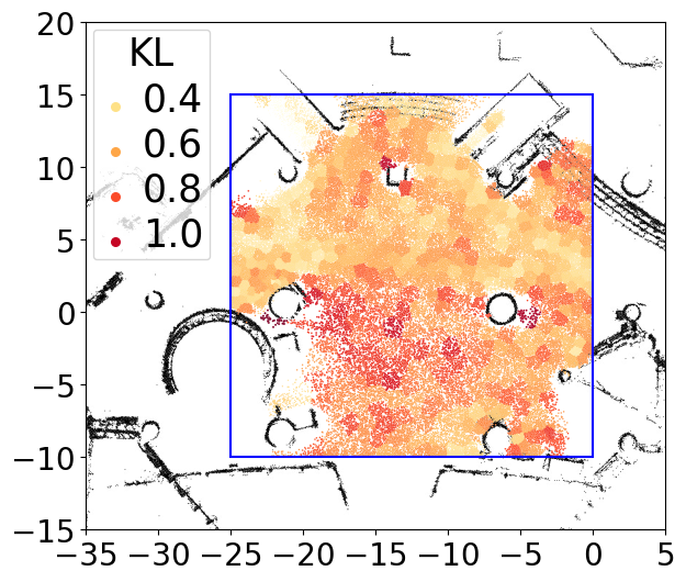
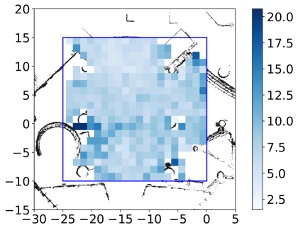
Figure 4: Left: KL divergence between $\Gamma^{R}$ and $\Gamma^{L}$. Right: A heatmap illustrating the FDE values of LaCE-LHMP in the ATC dataset, with a prediction horizon of $20\text{\,}\mathrm{s}$. Predictions exhibit higher accuracy in the central region. Predictions exhibit higher accuracy in the central region, which is predominantly laminar, as indicated by lower KL divergence.

V-A Quantitative results

We compare LaCE-LHMP with CLiFF-LHMP, T++, and CVM with prediction horizon from $1\text{\,}\mathrm{s}$ to $20\text{\,}\mathrm{s}$. Fig. 5 shows the quantitative results obtained in the ATC dataset described above. ADE/FDE and top-k ADE/FDE values for predictions using the LaCE-LHMP and baselines are presented. In the short-term perspective, all approaches perform on par. As the prediction horizon increases, LaCE-LHMP increasingly improves in terms of accuracy over baseline approaches. Notably, our method achieves significantly higher accuracy in the considered period. For the minimum ADE and FDE value from 5 randomly sampled trajectories, T++ has achieved better performance of top-k ADE/FDE, but in the long-term prediction horizon of $20\text{\,}\mathrm{s}$, our approach performs on par. With effective ranking of predicted trajectories, our method outperforms baselines in ADE/FDE values.

Table I summarises the performance results of our method against the baseline approaches at the maximum prediction horizon of $20\text{\,}\mathrm{s}$. At $20\text{\,}\mathrm{s}$ in the ATC dataset, our method achieves a 6.0% ADE and 6.4% FDE improvement in performance compared to CLiFF-LHMP, and 45.6% ADE and 46.1% FDE compared with Trajectron++. At the same time, LaCE-LHMP achieves a comparable top-k ADE and a slightly larger top-k FDE value compared with T++.

To evaluate the relation between prediction performance and the degree of laminar dominance in the environment, we present a heatmap of FDE values of our approach for prediction horizon $20\text{\,}\mathrm{s}$ in Fig. 4. In laminar-dominated regions, predictions made using the LaCE model are more accurate than in regions with more turbulent patterns, indicating that the former are more predictable.

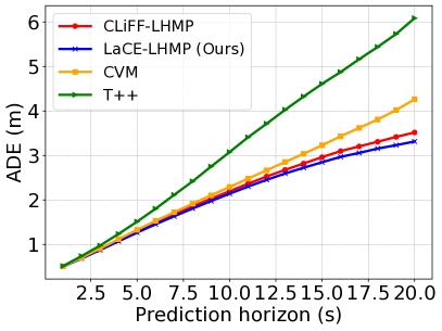
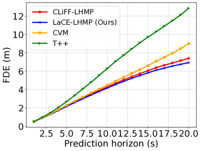
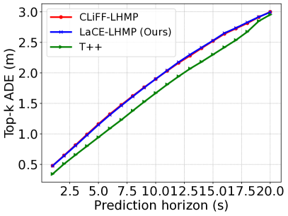
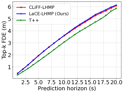
Figure 5: ADE/FDE (top) and top-k ADE/FDE (bottom) in the ATC dataset with a prediction horizon 1–$20\text{\,}\mathrm{s}$. Predictions with the LaCE model are more accurate during the whole considered period, as indicated by lower ADE/FDE values, which signify improved performance.

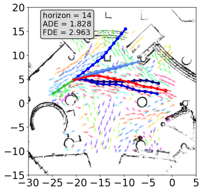
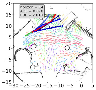
Figure 6: Two examples of predicted trajectory rankings using LaCE-LHMP. The red line represents the ground truth trajectory, the green line represents the observed trajectory and blue lines the predicted trajectories, with darker shades of blue indicating higher-ranked predictions. The LaCE model is shown in colored arrows. Predictions that align more closely with dominant flow patterns, and are thus darker in blue, demonstrate higher accuracy, showcasing the effectiveness of the ranking mechanism.

Figure 7: Prediction examples in ATC with $15\text{\,}\mathrm{s}$ prediction horizon. Red line represents the ground truth trajectory, green line represents the observed trajectory, and the blue lines represent the predicted trajectories. Upper-left: Prediction result of CVM, with the highest prediction error in this case. Upper-right: Prediction result of T++. As no explicit map is provided, the predicted trajectory might collide with obstacles. Lower-left: Prediction result of CLiFF-LHMP. Despite not using an obstacle map, the predicted trajectories avoid obstacles. CLiFF-LHMP captures multiple flow patterns, such as passing through stairs (top of the map) and moving to the right, resulting in a broader spread of predictions. Lower-right: Prediction result of LaCE-LHMP. Compared to the baselines, our approach better captures the dominant flow patterns. The generated trajectories are more concentrated, closely following the dominant flow and yielding a more accurate prediction.

V-B Qualitative results

We present the CLiFF-map and LaCE model depicting human flow patterns within the central area of the ATC dataset in Fig. 3. The CLiFF-map describes the human flow at a given location with a multimodal distribution, while the LaCE model reveals the dominant human flow patterns, achieved by estimating $\Gamma^{L}$ as a probabilistic representation of the Laminar component for each cluster. The difference between the two methods can be found in the bottom area in the middle of both subfigures in Fig. 3. Both the LaCE model and CLiFF-map present a horizontal human flow in the middle of the scene. While in the bottom area, from the LaCE model, one can observe a clear motion pattern originating from the top and progressing toward the bottom. In contrast, the corresponding area in the CLiFF-map exhibits a less distinct flow pattern.

Fig. 6 demonstrates ranking predicted trajectories using LaCE-LHMP. The predictions with a higher ranking (in a darker blue colour) align with the dominant flow pattern in the LaCE model and the highest-ranked prediction is closer to the ground truth. We present examples of predictions in Fig. 7. With CLiFF-map, the predictions exhibit a spread due to the multimodal distribution within the map. In contrast, predictions made with the LaCE model result in more concentrated trajectories, aligning with the dominant flow patterns observed in the middle area of the LaCE model.

VI CONCLUSION

In this study, we introduce a novel approach inspired by airflow modelling to tackle the challenging problem of long-term human motion prediction (LHMP). Our proposed Laminar Component Enhanced (LaCE) LHMP approach is designed to extract the laminar component of human trajectories, creating a probabilistic representation of the underlying streamlined and predictable flows. This approach improves the prediction of future motion patterns substantially. In addition to the laminar flow component extraction, another key innovation of the LaCE approach is its utilization of KL-divergence to quantitatively measure the laminar-dominant condition, allowing for adaptive adjustments to the contribution of the laminar component in the prediction process. The degree of laminar dominance can indicate the level of predictability of human motion in the environment.

The promising results in a benchmark against the prior art LHMP methods 1) confirm that laminar flow is a useful category to analyze real-world human trajectories; 2) support our hypothesis that laminar flow components are distinguishable in human motion patterns; 3) demonstrate the superior prediction performance of the LaCE-LHMP approach; and 4) show that laminar-dominant measurement can quantitatively indicate the predictability of the regions, contribute to a better understanding of human movement patterns.

In the future work, we intend to study more closely the turbulent component of the model, which can be used to describe, detect and predict abnormal behavior.

References

- [1] Andrey Rudenko, Luigi Palmieri, Michael Herman, Kris M Kitani, Dariu M Gavrila and Kai O Arras “Human motion trajectory prediction: A survey” In Int. J. of Robotics Research 39.8 Sage Publications Sage UK: London, England, 2020, pp. 895–935
- [2] Andrey Rudenko, Luigi Palmieri, Achim J Lilienthal and Kai O Arras “Human motion prediction under social grouping constraints” In 2018 IEEE/RSJ International Conference on Intelligent Robots and Systems (IROS), 2018, pp. 3358–3364 IEEE
- [3] Tomasz Piotr Kucner et al. “Survey of maps of dynamics for mobile robots” In Int. J. of Robotics Research 42.11, 2023, pp. 977–1006
- [4] Yufei Zhu, Andrey Rudenko, Tomasz P. Kucner, Luigi Palmieri, Kai O. Arras, Achim J. Lilienthal and Martin Magnusson “CLiFF-LHMP: Using Spatial Dynamics Patterns for Long- Term Human Motion Prediction” In Proc. of the IEEE Int. Conf. on Intell. Robots and Syst. (IROS), 2023
- [5] T.. Kucner, M. Magnusson, E. Schaffernicht, V.. Bennetts and A.. Lilienthal “Enabling Flow Awareness for Mobile Robots in Partially Observable Environments” In IEEE Robotics and Automation Letters 2.2, 2017, pp. 1093–1100
- [6] Yufei Zhu, Andrey Rudenko, Tomasz P Kucner, Achim J Lilienthal and Martin Magnusson “A Data-Efficient Approach for Long-Term Human Motion Prediction Using Maps of Dynamics” In arXiv preprint arXiv:2306.03617, 2023
- [7] W. Liu, D. W. and S. Gao “Future Frame Prediction for Anomaly Detection – A New Baseline” In Proc. of the IEEE Conf. on Comp. Vis. and Pat. Rec. (CVPR), 2018
- [8] Tharindu Fernando, Simon Denman, Sridha Sridharan and Clinton Fookes “Soft+Hardwired attention: An LSTM framework for human trajectory prediction and abnormal event detection” In Neural networks 108 Elsevier, 2018, pp. 466–478
- [9] Victor Hernandez Bennetts, Tomasz Piotr Kucner, Erik Schaffernicht, Patrick P Neumann, Han Fan and Achim J Lilienthal “Probabilistic air flow modelling using turbulent and laminar characteristics for ground and aerial robots” In IEEE Robotics and Automation Letters 2.2 IEEE, 2017, pp. 1117–1123
- [10] ASHRAE Handbook ASHRAE “Fundamentals, SI ed” In American Society of Heating, Refrigerating and Air-Conditioning Engineers, Atlanta, GA 2017, 2017
- [11] Con Doolan and Danielle Moreau “Laminar and Turbulent Flow” In Flow Noise: Theory Springer, 2022, pp. 71–105
- [12] A. Alahi, K. Goel, V. Ramanathan, A. Robicquet, L. Fei-Fei and S. Savarese “Social LSTM: Human trajectory prediction in crowded spaces” In Proc. of the IEEE Conf. on Comp. Vis. and Pat. Rec. (CVPR), 2016, pp. 961–971
- [13] Yujiao Cheng, Weiye Zhao, Changliu Liu and Masayoshi Tomizuka “Human motion prediction using semi-adaptable neural networks” In 2019 American Control Conference (ACC), 2019, pp. 4884–4890 IEEE
- [14] Fabio Carrara, Petr Elias, Jan Sedmidubsky and Pavel Zezula “LSTM-based real-time action detection and prediction in human motion streams” In Multimedia Tools and Applications 78 Springer, 2019, pp. 27309–27331
- [15] Abduallah Mohamed, Kun Qian, Mohamed Elhoseiny and Christian Claudel “Social-stgcnn: A social spatio-temporal graph convolutional neural network for human trajectory prediction” In Proc. of the IEEE Conf. on Comp. Vis. and Pat. Rec. (CVPR), 2020, pp. 14424–14432
- [16] Dapeng Zhao and Jean Oh “Noticing motion patterns: A temporal cnn with a novel convolution operator for human trajectory prediction” In IEEE Robotics and Automation Letters 6.2 IEEE, 2020, pp. 628–634
- [17] Guo Xie, Anqi Shangguan, Rong Fei, Wenjiang Ji, Weigang Ma and Xinhong Hei “Motion trajectory prediction based on a CNN-LSTM sequential model” In Science China Information Sciences 63 Springer, 2020, pp. 1–21
- [18] Xiaoli Liu, Jianqin Yin, Jin Liu, Pengxiang Ding, Jun Liu and Huaping Liu “Trajectorycnn: a new spatio-temporal feature learning network for human motion prediction” In IEEE Transactions on Circuits and Systems for Video Technology 31.6 IEEE, 2020, pp. 2133–2146
- [19] Amir Sadeghian, Vineet Kosaraju, Ali Sadeghian, Noriaki Hirose and Silvio Savarese “SoPhie: An attentive GAN for predicting paths compliant to social and physical constraints” In Proc. of the IEEE Conf. on Comp. Vis. and Pat. Rec. (CVPR), 2019, pp. 1349–1358
- [20] Fang Fang, Pengpeng Zhang, Bo Zhou, Kun Qian and Yahui Gan “Atten-GAN: Pedestrian Trajectory Prediction with GAN Based on Attention Mechanism” In Cognitive Computation 14.6 Springer, 2022, pp. 2296–2305
- [21] Tim Salzmann, Boris Ivanovic, Punarjay Chakravarty and Marco Pavone “Trajectron++: Dynamically-Feasible Trajectory Forecasting With Heterogeneous Data” In Proc. of the Europ. Conf. on Comp. Vision (ECCV), 2020, pp. 683–700
- [22] Hao Zhou, Dongchun Ren, Xu Yang, Mingyu Fan and Hai Huang “Sliding sequential CVAE with time variant socially-aware rethinking for trajectory prediction” In arXiv preprint arXiv:2110.15016, 2021
- [23] Pei Xu, Jean-Bernard Hayet and Ioannis Karamouzas “Socialvae: Human trajectory prediction using timewise latents” In European Conference on Computer Vision, 2022, pp. 511–528 Springer
- [24] Francesco Giuliari, Irtiza Hasan, Marco Cristani and Fabio Galasso “Transformer networks for trajectory forecasting” In Proc. of the IEEE Int. Conf. on Pattern Recognition, 2021, pp. 10335–10342 IEEE
- [25] Christoph Schöller, Vincent Aravantinos, Florian Lay and Alois Knoll “What the constant velocity model can teach us about pedestrian motion prediction” In IEEE Robotics and Automation Letters 5.2 IEEE, 2020, pp. 1696–1703
- [26] D. Helbing and P. Molnar “Social force model for pedestrian dynamics” In Physical review E 51.5 APS, 1995, pp. 4282
- [27] M. Luber, J.. Stork, G.. Tipaldi and K.. Arras “People tracking with human motion predictions from social forces” In Proc. of the IEEE Int. Conf. on Robotics and Automation (ICRA), 2010, pp. 464–469
- [28] F. Farina, D. Fontanelli, A. Garulli, A. Giannitrapani and D. Prattichizzo “Walking Ahead: The Headed Social Force Model” In PloS one 12.1 Public Library of Science, 2017, pp. e0169734
- [29] J. Berg, M. Lin and D. Manocha “Reciprocal velocity obstacles for real-time multi-agent navigation” In Proc. of the IEEE Int. Conf. on Robotics and Automation (ICRA), 2008, pp. 1928–1935
- [30] Jur Van Den Berg, Stephen J Guy, Ming Lin and Dinesh Manocha “Reciprocal n-body collision avoidance” In Proc. of the Int. Symp. of Robotics Research (ISRR), 2011, pp. 3–19 Springer
- [31] J… Kooij, F. Flohr, E… Pool and D.. Gavrila “Context-Based Path Prediction for Targets with Switching Dynamics” In Int. J. of Comp. Vision (IJCV) 127.3, 2019, pp. 239–262
- [32] B.. Ziebart, N. Ratliff, G. Gallagher, C. Mertz, K. Peterson, J.. Bagnell, M. Hebert, A.. Dey and S. Srinivasa “Planning-based prediction for pedestrians” In Proc. of the IEEE Int. Conf. on Intell. Robots and Syst. (IROS), 2009, pp. 3931–3936
- [33] A. Rudenko, L. Palmieri and K.. Arras “Joint Prediction of Human Motion Using a Planning-Based Social Force Approach” In Proc. of the IEEE Int. Conf. on Robotics and Automation (ICRA), 2018, pp. 1–7
- [34] E. Rehder, F. Wirth, M. Lauer and C. Stiller “Pedestrian prediction by planning using deep neural networks” In Proc. of the IEEE Int. Conf. on Robotics and Automation (ICRA), 2018, pp. 1–5
- [35] P. Coscia, F. Castaldo, F… Palmieri, A. Alahi, S. Savarese and L. Ballan “Long-term path prediction in urban scenarios using circular distributions” In Image and Vision Computing 69 Elsevier, 2018, pp. 81–91
- [36] Karttikeya Mangalam, Yang An, Harshayu Girase and Jitendra Malik “From Goals, Waypoints & Paths To Long Term Human Trajectory Forecasting” In Proc. of the IEEE Int. Conf. on Computer Vision (ICCV), 2021, pp. 15213–15222
- [37] Sebastian Thrun “Probabilistic robotics” In Communications of the ACM 45.3 ACM New York, NY, USA, 2002, pp. 52–57
- [38] Dražen Brščić, Takayuki Kanda, Tetsushi Ikeda and Takahiro Miyashita “Person tracking in large public spaces using 3-D range sensors” In IEEE Transactions on Human-Machine Systems 43.6 IEEE, 2013, pp. 522–534
- [39] Andrey Rudenko, Luigi Palmieri, Wanting Huang, Achim J Lilienthal and Kai O Arras “The Atlas Benchmark: an Automated Evaluation Framework for Human Motion Prediction” In Proc. of the IEEE Int. Symp. on Robot and Human Interactive Comm. (RO-MAN), 2022