Accurate Power Spectrum Estimation toward Nyquist limit

Abstract

The power spectrum, as a statistic in Fourier space, is commonly numerically calculated using the fast Fourier transform method to efficiently reduce the computational costs. To alleviate the systematic bias known as aliasing due to the insufficient sampling, the interlacing technique was proposed. We derive the analytical form of the shot noise under the interlacing technique, which enables the exact separation of the Poisson shot noise from the signal in this case. Thanks to the accurate shot noise subtraction, we demonstrate an enhancement in the accuracy of power spectrum estimation, and compare with the other widely used estimators in community. The good performance of our estimation allows an abatement in the computational cost by using low resolution and low order mass assignment scheme in the analysis for huge surveys and mocks.

1 Introduction

The power spectrum, usually denoted as $P(k)$ for three dimensional space, is an important statistical quantity in cosmological research. It is the Fourier transform pair of the two-point correlation function and reflects the magnitude of the matter density fluctuations at different spatial scales. The most accurate power spectrum estimation is the direct summation [9], but it is very time consuming as the computational cost is proportional to the number of grid points in ${\boldsymbol{k}}$ space as well as the number of galaxies. Thus, the power spectrum is usually calculated using the Fast Fourier Transform (FFT) method. By factorizing the calculation to even and odd series recursively, FFT reduces the computational complexity from $\mathcal{O}(N^{2})$ to $\mathcal{O}(N\log N)$, with $N$ being the total number of grid points.

Under the FFT method, the approximations made introduce a series of systematic effects that need to be corrected. The FFT method requires us to sample the original catalogue at specific grid points for subsequent computations. This sampling process is known as the mass assignment scheme. On one hand, reconstructing a continuous signal from discrete samples requires an interpolation scheme to preserve the sampling, and the choice of interpolation kernel is related to the mass assignment scheme used. The deviation caused by the variation in the mass assignment function is known as the window function effect, which needs to be corrected by the deconvolution. On the other hand, representing a continuous mass distribution by a discrete mass distribution introduces inherent background noise known as shot noise effect. On top of the two, the maximum frequency we can sample is determined by the frequency corresponding to the separation of grid points, and any signal with frequencies higher than this cannot be measured. According to the Shannon sampling theorem, in order to faithfully recover the original signal without loss or distortion, the sampling frequency must be higher than twice the maximum frequency component of the original signal, which requires a truncation of the signal at high frequencies. However, when analyzing large-scale structures, the frequencies of cosmological perturbations typically exceed the Nyquist frequency in the analysis, causing high-frequency components to be erroneously folded into the part within the sampling frequency range. This systematic error caused by the finite sampling frequency is known as aliasing. Among these systematic errors, the window function effect and shot noise effect are independent of the distribution of the sample and can be precisely solved and eliminated. The analytical expressions for the window function term and shot noise correction term was provided in [7]. On the contrary, the bias resulting from aliasing is related to the signal itself, and is difficult to remove without prior knowledge.

To mitigate the contamination of the signal by aliasing, one approach is to apply a low-pass filter to the signal before Fourier transformation. However, as a interpolation kernel, the computational cost of a low-pass filter increases with the rigor of the filter, making the advantage of using the FFT method for optimization and acceleration over direct summation less significant. In cosmological research, there have been various attempts to mitigate the effects of aliasing on power spectrum measurements. An iterative elimination method by assuming that the real power spectrum near Nyquist frequency can be approximated as a power law was proposed in [7]. For selecting the ideal window function to minimize sampling effects certain criteria was proposed and the Daubechies wavelet transform-based window function is suggested as a candidate for minimizing sampling effects [3]. Based on the Daubechies 6 wavelet basis and third-order B-splines a mass assignment scheme was further proposed in [11]. Interlacing technique was proposed by [1], and later introduced in the $AP^{3}M$ N-body code [2]. Originally used in television signals or image processing, Interlacing is a method to enhance image or signal quality by effectively reducing aliasing effects using two interlaced grids with only twice the computational cost of standard operations, the reduction in systematic errors achieved by this method was quantified in [9].

In this paper, we focus on the precise derivation and elimination of the shot noise term under the interlacing technique, further improving the accuracy of the power spectrum estimation. The paper is organized as follows. Chapter 2 begins with an derivation of the analytical relationship between the power spectrum measurement from FFT and real signals. It also reviews common forms of power spectrum estimation in the literature and the assumptions underlying these estimation methods. In the third part of Chapter 2, the interlacing technique is introduced, explaining its principles for reducing aliasing effects. The precise form of the correct shot noise term under this technique is derived, highlighting its significance in capturing aliasing effects in the shot noise signal. Numerical tests are performed in Chapter 3 to quantify the obtained power spectrum using the various estimation methods discussed. The simulations provide evidence of the precision advantage of one of the estimators, especially at small scales, near the Nyquist frequency, and with lower-order window function sampling and lower sample particle density. This advantage is particularly important in future large-scale data analysis, as the sky coverage and volume occupation is dramatically increased so that computational efficiency is crucial. We summarize the results in Chapter 4.

2 Formulae and Estimators

2.1 Power spectrum estimator

We focus on a simulated halo catalogue within a periodical cubic box of volume $V=L^{3}$. $L$ represents the physical/comoving size of the box. For the power spectrum calculation, first we need to use a mass assignment scheme to convert a catalogue to a field. Usually, Nearest Grid Point (NGP), Cloud-In-Cell (CIC), Triangular Shaped Cloud (TSC) and Piecewise Cubic Spline (PCS) scheme is adopted. We refer the readers to [9] for the real space kernels of the above mass assignments. We express the halo number density $n({\boldsymbol{x}})$ in a dimensionless form

$$\delta^{f}({\boldsymbol{x}})=\frac{n^{f}({\boldsymbol{x}})}{\bar{n}}-1\ ,$$ (2.1)

where $\bar{n}$ is the mean density within the volume $V$, and the superscript $f$ represents that the density field is sampled using one of the above mass assignment scheme. Under the condition of periodicity, we Fourier transform the overdensity field,

$$\delta^{f}({\boldsymbol{k}})=\frac{1}{V}\int_{V}{\delta^{f}({\boldsymbol{x}})e^{i{\boldsymbol{k}}\cdot{\boldsymbol{x}}}d{\boldsymbol{x}}\ .}$$ (2.2)

In Fourier space, the mass assignment schemes induce window effect on the resulting field,

$$W({\boldsymbol{k}})=\left[\frac{\sin(\pi k_{1}/k_{H})}{\pi k_{1}/k_{H}}\frac{\sin(\pi k_{2}/k_{H})}{\pi k_{2}/k_{H}}\frac{\sin(\pi k_{3}/k_{H})}{\pi k_{3}/k_{H}}\right]^{p}\ .$$ (2.3)

For NGP, CIC, TSC and PSC, $p=1,2,3$ and $4$, respectively. $k_{H}=\frac{2\pi N_{g}}{L}$ represents the spatial frequency corresponding to the minimum grid point distance, and $N_{g}$ represents the number of grid points in one dimension. Following the derivation, conventions and expressions in [7], the resulting power spectrum is

$$\langle|\delta^{f}({\boldsymbol{k}})|^{2}\rangle =\sum_{\boldsymbol{n}}|W({\boldsymbol{k}}+k_{H}{\boldsymbol{n}})|^{2}P({\boldsymbol{k}}+k_{H}{\boldsymbol{n}})+\frac{1}{N}\sum_{\boldsymbol{n}}|W({\boldsymbol{k}}+k_{H}{\boldsymbol{n}})|^{2}\ .$$ (2.4)

We refer the first term in the r.h.s. of Eq. (2.4) as the signal term. It is the summation of the power spectrum with window effect over a series of shifted images, which is known as aliasing. The ${\boldsymbol{n}}\neq 0$ components represent the contribution of aliased images, which boosts the power near Nyquist frequency if the sampling rate is not sufficiently high. The last term in Eq. (2.4) is the shot noise contribution. Note that the shot noise $1/N$ also suffers from the window function and aliasing effect.

2.2 No interlacing

As in [7], we denote the shot noise term as $\frac{1}{N}C({\boldsymbol{k}})\equiv\frac{1}{N}\sum_{\boldsymbol{n}}|W({\boldsymbol{k}}+k_{H}{\boldsymbol{n}})|^{2}$. From the identity

$$\sum_{n}\frac{1}{(x-\pi n)^{q}}=\frac{(-1)^{q-1}}{{(q-1)}!}\frac{d^{q-1}}{dx^{q-1}}\cot x\ ,$$ (2.5)

the summation over infinite images of $W$ in one dimension can be derived. Let $q=2p$ and $x=\pi k/k_{H}$,

$$\sum_{n}|W(k+k_{H}n)|^{2} =\sum_{n}\left(\frac{\sin(\pi k/k_{H}+n\pi)}{\pi k/k_{H}+n\pi}\right)^{2p}$$ (2.6)

$$=\sin^{2p}(x)\sum_{n}\frac{1}{(x+n\pi)^{2p}}$$

$$={\sin^{q}x}\frac{(-1)^{q-1}}{{(q-1)}!}\frac{d^{q-1}}{dx^{q-1}}\cot x\ .$$

We denote the result as $S_{q}[\sin^{2}x]$ since it is a polynomial function of $\sin^{2}x$ up to order of $p-1$.

$$S_{q}[\sin^{2}x] =\left\{\begin{aligned} &1\ ,&\text{NGP}\ ,\\ &1-\frac{2}{3}\sin^{2}x\ ,&\text{CIC}\ ,\\ &1-\sin^{2}x+\frac{2}{15}\sin^{4}x\ ,&\text{TSC}\ ,\\ &1-\frac{4}{3}\sin^{2}x+\frac{2}{5}\sin^{4}x-\frac{4}{315}\sin^{6}x\ ,&\text{PSC}\ .\\ \end{aligned}\right.$$ (2.7)

Thus, $C({\boldsymbol{k}})$ has the exact analytical expression

$$C({\boldsymbol{k}})=\left\{\begin{aligned} &1\ ,&\text{NGP}\ ,\\ &\prod_{i}\left[1-\frac{2}{3}\sin^{2}\left(\frac{\pi k_{i}}{k_{H}}\right)\right]\ ,&\text{CIC}\ ,\\ &\prod_{i}\left[1-\sin^{2}\left(\frac{\pi k_{i}}{k_{H}}\right)+\frac{2}{15}\sin^{4}\left(\frac{\pi k_{i}}{k_{H}}\right)\right]\ ,&\text{TSC}\ ,\\ &\prod_{i}\left[1-\frac{4}{3}\sin^{2}\left(\frac{\pi k_{i}}{k_{H}}\right)+\frac{2}{5}\sin^{4}\left(\frac{\pi k_{i}}{k_{H}}\right)-\frac{4}{315}\sin^{6}\left(\frac{\pi k_{i}}{k_{H}}\right)\right]\ ,&\text{PSC}\ .\\ \end{aligned}\right.$$ (2.8)

We emphasize that the shot noise term can be precisely subtracted from Eq. (2.4). The isotropic versions of the shot noise term $C(k)$ except for the PSC scheme are provided in [7], and we also list the isotropic versions in the Appendix.

Neglecting the contamination from aliased images on the signal, i.e. assuming that $\sum_{\boldsymbol{n}}|W({\boldsymbol{k}}+k_{H}{\boldsymbol{n}})|^{2}P({\boldsymbol{k}}+k_{H}{\boldsymbol{n}})\approx P({\boldsymbol{k}})|W({\boldsymbol{k}})|^{2}$, a straightforward estimator is

$$\hat{P}({\boldsymbol{k}})=\frac{\langle|\delta^{f}({\boldsymbol{k}})|^{2}\rangle-\frac{1}{N}C({\boldsymbol{k}})}{|W({\boldsymbol{k}})|^{2}}\ .$$ (2.9)

In this estimator proposed in [7], the shot noise term is subtracted precisely before correcting the window function in the signal term. We expect that the discarded summation leads to the aliasing effect, a boost of the power spectrum amplitude near the Nyquist frequency.

Under a different approximation $\sum_{\boldsymbol{n}}|W({\boldsymbol{k}}+k_{H}{\boldsymbol{n}})|^{2}P({\boldsymbol{k}}+k_{H}{\boldsymbol{n}})\approx P({\boldsymbol{k}})\sum_{\boldsymbol{n}}|W({\boldsymbol{k}}+k_{H}{\boldsymbol{n}})|^{2}=P({\boldsymbol{k}})C({\boldsymbol{k}})$, and thus $\langle|\delta^{f}({\boldsymbol{k}})|^{2}\rangle\approx[P({\boldsymbol{k}})+\frac{1}{N}]C({\boldsymbol{k}})$, the corresponding estimator is

$$\hat{P}({\boldsymbol{k}})=\frac{\langle|\delta^{f}({\boldsymbol{k}})|^{2}\rangle}{C({\boldsymbol{k}})}-\frac{1}{N}\ .$$ (2.10)

For this estimator, the window effect is corrected first and the $1/N$ shot noise is subtracted in the end. We caution the readers that the window effect here is $C({\boldsymbol{k}})$ instead of $W^{2}({\boldsymbol{k}})$. This correction can be performed on the field level, by dividing the effective window function $\sqrt{C({\boldsymbol{k}})}$ from the Fourier transformed field $\delta({\boldsymbol{k}})$. 0This is also the approach adopted in Nbodykit [5] for the power spectrum estimation without interlacing technique.

2.3 Interlacing technique

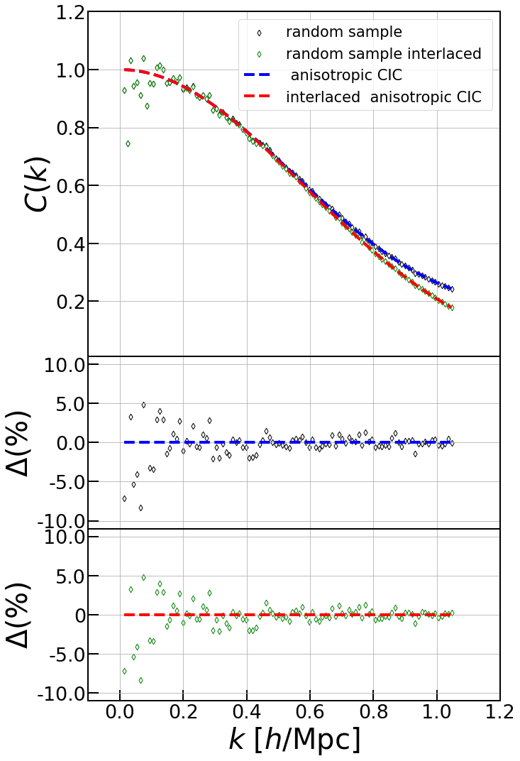
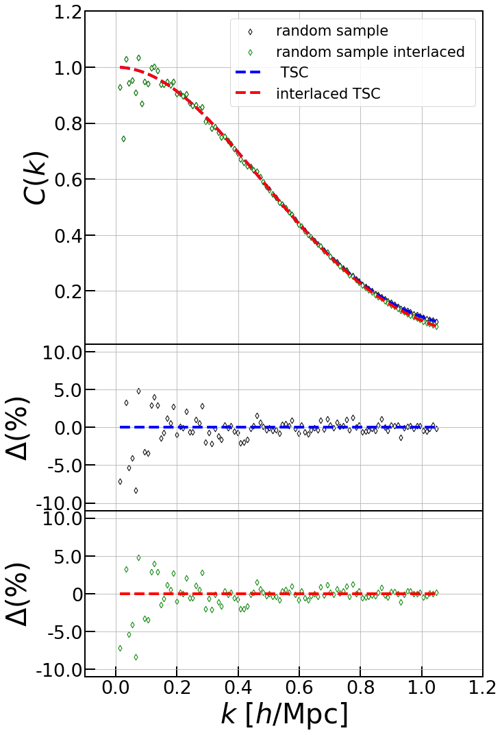
Figure 1: Shot noise estimated from Poisson-distributed random samples. On the left side are the results for the CIC window function, and on the right side are the results for the TSC window function. In the top panels the scattered points represent the $\langle\delta^{f}(k)^{2}\rangle$ obtained from the random sample, the blue dashed lines follow Eq. (2.8) and the red lines follow Eq. (2.15). The middle panels show the results scaled to the Eq. (2.8) and to the Eq. (2.15) for the bottom panels. The analytical expressions well describe the shot noise with interlacing technique.

Hockney and Eastwood, [6] proposed the interlacing technique, which was lately applied to the $AP^{3}M$ N-body code [2]. This technique samples the signals twice with the second mesh having an overall half-cell offset $(H/2,H/2,H/2)$ relative to the primary mesh. The odd terms in the aliasing images will be eliminated by taking the arithmetic average of the two samplings. As such, the effects of aliasing can be reduced, leading to an improved estimation of the power spectrum. We denote the average of the two samplings as $\tilde{\delta}^{f}({\boldsymbol{k}})$, and mathematically,

$$\tilde{\delta}^{f}({\boldsymbol{k}}) =\frac{1}{2}\left[\delta^{f}_{1}({\boldsymbol{k}})+\delta^{f}_{2}({\boldsymbol{k}})\right]$$ (2.11)

$$=\frac{1}{2}\left[\delta^{f}_{1}({\boldsymbol{k}})+\delta^{f}_{2}({\boldsymbol{k}}^{\prime})e^{-\mathrm{i}{\boldsymbol{k}}^{\prime}\cdot\boldsymbol{H}/2}\right]$$

$$=\sum_{\boldsymbol{n}}{\theta_{\boldsymbol{n}}{\delta}^{f}({\boldsymbol{k}}+k_{H}{\boldsymbol{n}})}\ .$$

Here, $\theta_{\boldsymbol{n}}$ constitutes an equivalent expression of the interlacing scheme in the algebraic space, defined as

$$\theta_{\boldsymbol{n}} \equiv\frac{1}{2}(1+(-1)^{n_{x}+n_{y}+n_{z}})$$ (2.12)

$$=\left\{\begin{array}[]{ll}1\ ,&n_{x}+n_{y}+n_{z}\text{ is even}\ ,\\ 0\ ,&n_{x}+n_{y}+n_{z}\text{ is odd}\ .\\ \end{array}\right.$$

Again, ${\boldsymbol{n}}=0$ is the true signal term. In most cases and also true for cosmological matter power spectrum, the signal decreases with increasing scale, and thus the most dominant contribution is from $|{\boldsymbol{n}}|=1$. With the interlacing technique above, the aliasing effect from all odd pixels is eliminated. This approach smooths the sampling near the Nyquist frequency. At the same time, it should be noted that the shot noise is also affected by this smoothing effect.

The shot noise term with interlacing is $C^{{\operatorname{int}}}({\boldsymbol{k}})=\sum_{{\boldsymbol{n}}}\theta_{\boldsymbol{n}}|W({\boldsymbol{k}}+k_{H}{\boldsymbol{n}})|^{2}$, in other words we are now interested in the summation of $\sum_{\boldsymbol{n}}|W({\boldsymbol{k}}+k_{H}{\boldsymbol{n}})|^{2}$ but over even $n_{x}+n_{y}+n_{z}$ terms. These terms can be split into two groups: all the $n_{i}$’s are even, or two of the three $n_{i}$’s are odd. Let $n=2m$, the summation over even terms in Eq. (2.6) is reduced to

$$C_{e}(x) \equiv\sum_{n\text{ is even}}\frac{\sin^{2p}(x+\pi n)}{(x+\pi n)^{2p}}=\sum_{m}\frac{\sin^{2p}(x+2\pi m)}{(x+2\pi m)^{2p}}=\frac{1}{2^{2p}}\frac{\sin^{2p}(x)}{\sin^{2p}(x/2)}S_{2p}[\sin^{2}(x/2)]$$ (2.13)

$$=\cos^{q}(x/2)S_{q}[\sin^{2}(x/2)]$$

$$=\left\{\begin{aligned} &\cos^{2}\left(\frac{x}{2}\right)\ ,&\text{NGP}\ ,\\ &\cos^{4}\left(\frac{x}{2}\right)\left[1-\frac{2}{3}\sin^{2}\left(\frac{x}{2}\right)\right]\ ,&\text{CIC}\ ,\\ &\cos^{6}\left(\frac{x}{2}\right)\left[1-\sin^{2}\left(\frac{x}{2}\right)+\frac{2}{15}\sin^{4}\left(\frac{x}{2}\right)\right]\ ,&\text{TSC}\ ,\\ &\cos^{8}\left(\frac{x}{2}\right)\left[1-\frac{4}{3}\sin^{2}\left(\frac{x}{2}\right)+\frac{2}{5}\sin^{4}\left(\frac{x}{2}\right)-\frac{4}{315}\sin^{6}\left(\frac{x}{2}\right)\right]\ ,&\text{PSC}\ .\\ \end{aligned}\right.$$

Here, $x=\frac{\pi k}{k_{H}}$. A similar derivation of the above relation is shown in [9] to obtain the relation between the residuals of the power spectrum estimator with and without interlacing. The summation over odd terms can be derived by letting $n=2m+1$,

$$C_{o}(x) \equiv\sum_{n\text{ is odd}}\frac{\sin^{2p}(x+\pi n)}{(x+\pi n)^{2p}}$$ (2.14)

$$=\sum_{m}\frac{\sin^{2p}(x+\pi+2\pi m)}{(x+\pi+2\pi m)^{2p}}=\frac{1}{2^{2p}}\frac{\sin^{2p}(x+\pi)}{\sin^{2p}(\frac{x+\pi}{2})}S_{2p}[\sin^{2}(\frac{x+\pi}{2})]$$

$$=\cos^{2p}\left(\frac{x+\pi}{2}\right)S_{2p}\left[\sin^{2}\left(\frac{x+\pi}{2}\right)\right]=\sin^{q}(x/2)S_{q}[\cos^{2}(x/2)]$$

$$=\left\{\begin{aligned} &\sin^{2}\left(\frac{x}{2}\right)\ ,&\text{NGP}\ ,\\ &\sin^{4}\left(\frac{x}{2}\right)\left[1-\frac{2}{3}\cos^{2}\left(\frac{x}{2}\right)\right]\ ,&\text{CIC}\ ,\\ &\sin^{6}\left(\frac{x}{2}\right)\left[1-\cos^{2}\left(\frac{x}{2}\right)+\frac{2}{15}\cos^{4}\left(\frac{x}{2}\right)\right]\ ,&\text{TSC}\ ,\\ &\sin^{8}\left(\frac{x}{2}\right)\left[1-\frac{4}{3}\cos^{2}\left(\frac{x}{2}\right)+\frac{2}{5}\cos^{4}\left(\frac{x}{2}\right)-\frac{4}{315}\cos^{6}\left(\frac{x}{2}\right)\right]\ ,&\text{PSC}\ .\\ \end{aligned}\right.$$

Thus, the exact shot noise term with interlacing is

$$C^{{\operatorname{int}}}({\boldsymbol{k}})=\prod_{i}C_{e}\left(\frac{\pi k_{i}}{k_{H}}\right)+\sum_{(i,j,m)\in A_{3}}C_{e}\left(\frac{\pi k_{i}}{k_{H}}\right)C_{o}\left(\frac{\pi k_{j}}{k_{H}}\right)C_{o}\left(\frac{\pi k_{m}}{k_{H}}\right)\ .$$ (2.15)

Here, the summation in the second term is over $A_{3}$, the alternating group of degree $3$, which collects the contributions from $(i,j,m)=(1,2,3),(2,3,1)$ and $(3,1,2)$.

To exam the accuracy of the above shot noise formula, we calculate the power spectrum of a random sample with number density of $n_{s}=1.12\times 10^{-3}\text{ Mpc}^{-3}h^{3}$. We show the performance of the Eq. (2.15) in Figure 1, along with the result for Eq. (2.8) (also appeared in [7]). The analytical expressions describe the data points from the numerical calculation well, with the residual scattering around the expectation. The accuracy of the interlaced shot noise formula lines up with the accuracy of the case without interlacing.

The first term in Eq. (2.15) is usually larger than the second term which includes sine functions from two odd terms. This very expression of the leading term is similar to Eq. (2.7), with $\sin^{2}x$ being replaced by $\sin^{2}(x/2)$ and an extra cosine prefactors $\cos^{2p}(x/2)$ induced by interlacing. Notice that for NGP mass assignment without interlacing, the aliasing effect exactly compensates the window effect, leading to exactly $1/N$ shot noise power. However, when interlacing is adopted, the shot noise for NGP is lower than $1/N$ at small scale. Naively using $1/N$ as the shot noise like Eq. (2.9) leads to an over-subtraction of the shot noise.

Under the same approximation, $\sum_{\boldsymbol{n}}|W({\boldsymbol{k}}+k_{H}{\boldsymbol{n}})|^{2}P({\boldsymbol{k}}+k_{H}{\boldsymbol{n}})\approx P({\boldsymbol{k}})|W({\boldsymbol{k}})|^{2}$ in deriving the estimator Eq. (2.9), the new estimator for interlacing is

$$\hat{P}({\boldsymbol{k}})=\frac{\langle|\tilde{\delta}^{f}({\boldsymbol{k}})|^{2}\rangle-\frac{1}{N}C^{{\operatorname{int}}}({\boldsymbol{k}})}{|W({\boldsymbol{k}})|^{2}}\ .$$ (2.16)

Again, in this estimator the shot noise term is subtracted precisely before correcting the window function in the signal term. Since aliasing is significantly reduced by the interlacing technique, an accurate shot noise subtraction is essential to avoid the systematic bias.

The interlacing technique reduces aliasing both in the signal term and in the shot noise term. Under this consideration, we can directly discard the summation as $\sum_{\boldsymbol{n}}|W({\boldsymbol{k}}+k_{H}{\boldsymbol{n}})|^{2}\left[P({\boldsymbol{k}}+k_{H}{\boldsymbol{n}})+\frac{1}{N}\right]\approx[P({\boldsymbol{k}})+\frac{1}{N}]|W({\boldsymbol{k}})|^{2}$, and thus the corresponding estimator is

$$\hat{P}({\boldsymbol{k}})=\frac{\langle|\tilde{\delta}^{f}({\boldsymbol{k}})|^{2}\rangle}{|W({\boldsymbol{k}})|^{2}}-\frac{1}{N}\ .$$ (2.17)

In this estimator, the shot noise can be easily separated as a constant term throughout the entire computation process, which is also the power spectrum calculation approach in Nbodykit [5] for interlacing. Comparing this estimation with Eq. (2.16), it can be observed that the shot noise assumed here is $\frac{1}{N}W^{2}({\boldsymbol{k}})$ instead of $\frac{1}{N}C^{{\operatorname{int}}}(\mathbf{k})$. Although the difference between these two assumed shot noise forms is small, the approach in Eq. (2.17) still underestimates the contribution of shot noise, leading to an overestimation of the power spectrum. We summarize the above four estimators in Table 1.

Note that the interlacing technique here refers to use 2 interlaced grids, which eliminates the main contamination from $|{\boldsymbol{n}}|=1$. To eliminate more images, we have to use more interlaced grids. In Appendix B, we also provide the analytical shot noise expressions with multiple interlaced grids and various mass assignment schemes.

Table 1: The summary of the assumptions and properties of various power spectrum estimators. The first two rows do not involve interlacing and the last two adopt interlacing. For the estimators in the first and third row, the shot noise is precisely subtracted first, then the window effect is deconvolved. For the estimators in the second and fourth row, the window effect is deconvolved at field level, then the shot noise is subtracted from the obtained power spectrum.

Approximation	Estimator	Description
$\sum_{\boldsymbol{n}}|W({\boldsymbol{k}}+k_{H}{\boldsymbol{n}})|^{2}P({\boldsymbol{k}}+k_{H}{\boldsymbol{n}})$ $\approx P({\boldsymbol{k}})|W({\boldsymbol{k}})|^{2}$	$\hat{P}({\boldsymbol{k}})=\frac{\langle|\delta^{f}({\boldsymbol{k}})|^{2}\rangle-\frac{1}{N}C({\boldsymbol{k}})}{|W({\boldsymbol{k}})|^{2}}$, Eq. (2.9)	Exact shot noise subtraction without interlacing.
$\sum_{\boldsymbol{n}}|W({\boldsymbol{k}}+k_{H}{\boldsymbol{n}})|^{2}P({\boldsymbol{k}}+k_{H}{\boldsymbol{n}})$ $\approx P({\boldsymbol{k}})\sum_{\boldsymbol{n}}|W({\boldsymbol{k}}+k_{H}{\boldsymbol{n}})|^{2}$	$\hat{P}({\boldsymbol{k}})=\frac{\langle|\delta^{f}({\boldsymbol{k}})|^{2}\rangle}{C({\boldsymbol{k}})}-\frac{1}{N}$, Eq. (2.10)	Window effect $\sqrt{C({\boldsymbol{k}})}$ can be deconvolved at field level.
$\sum_{\boldsymbol{n}}|W({\boldsymbol{k}}+k_{H}{\boldsymbol{n}})|^{2}P({\boldsymbol{k}}+k_{H}{\boldsymbol{n}})$ $\approx P({\boldsymbol{k}})|W({\boldsymbol{k}})|^{2}$	$\hat{P}({\boldsymbol{k}})=\frac{\langle|\tilde{\delta}^{f}({\boldsymbol{k}})|^{2}\rangle-\frac{1}{N}C^{{\operatorname{int}}}({\boldsymbol{k}})}{|W({\boldsymbol{k}})|^{2}}$, Eq. (2.16)	Exact shot noise subtraction for interlacing.
$\sum_{\boldsymbol{n}}|W({\boldsymbol{k}}+k_{H}{\boldsymbol{n}})|^{2}\left[P({\boldsymbol{k}}+k_{H}{\boldsymbol{n}})+\frac{1}{N}\right]$ $\approx\left[P({\boldsymbol{k}})+\frac{1}{N}\right]|W({\boldsymbol{k}})|^{2}$	$\hat{P}({\boldsymbol{k}})=\frac{\langle|\tilde{\delta}^{f}({\boldsymbol{k}})|^{2}\rangle}{|W({\boldsymbol{k}})|^{2}}-\frac{1}{N}$, Eq. (2.17)	Window effect $|W({\boldsymbol{k}})|$ can be deconvolved at field level.

3 Numerical Tests

We conduct the numerical tests on the halo samples simulated by Gadget-4 code [10]. The simulation box length is $L=600\,h^{-1}\mathrm{Mpc}$. The cosmological parameters employed here are: $\Omega_{m}=0.308$, $\Omega_{\Lambda}=0.692$, $\Omega_{b}=0.049$, $H_{0}=67.8\,{\rm km}\,s^{-1}\,\rm{Mpc}^{-1}$. The halo sample is generated by the on-the-fly Friends-of-Friends halo finder. The sample consists of a total of 2,413,300 dark matter halos with mass ranging from $3.40\times 10^{11}M_{\odot}/h$ to $7.30\times 10^{14}M_{\odot}/h$, located at a redshift of $z=1$.

3.1 Full halo sample

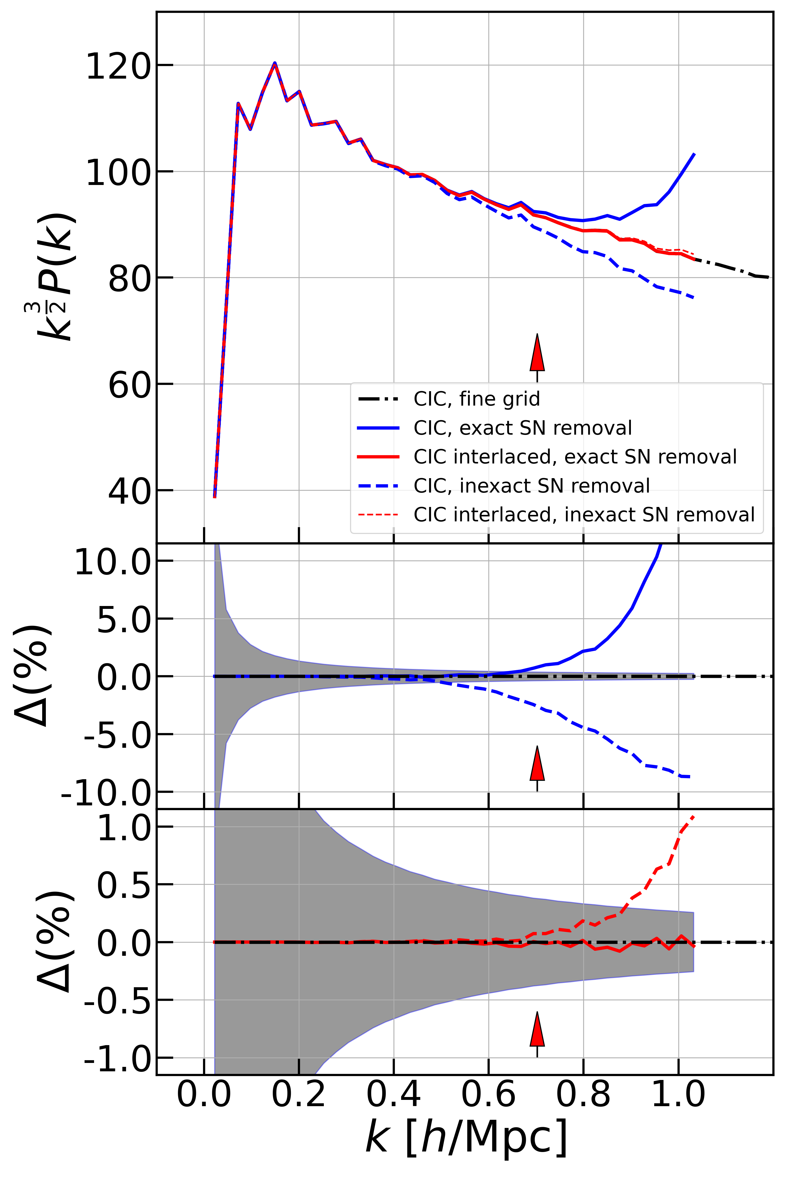
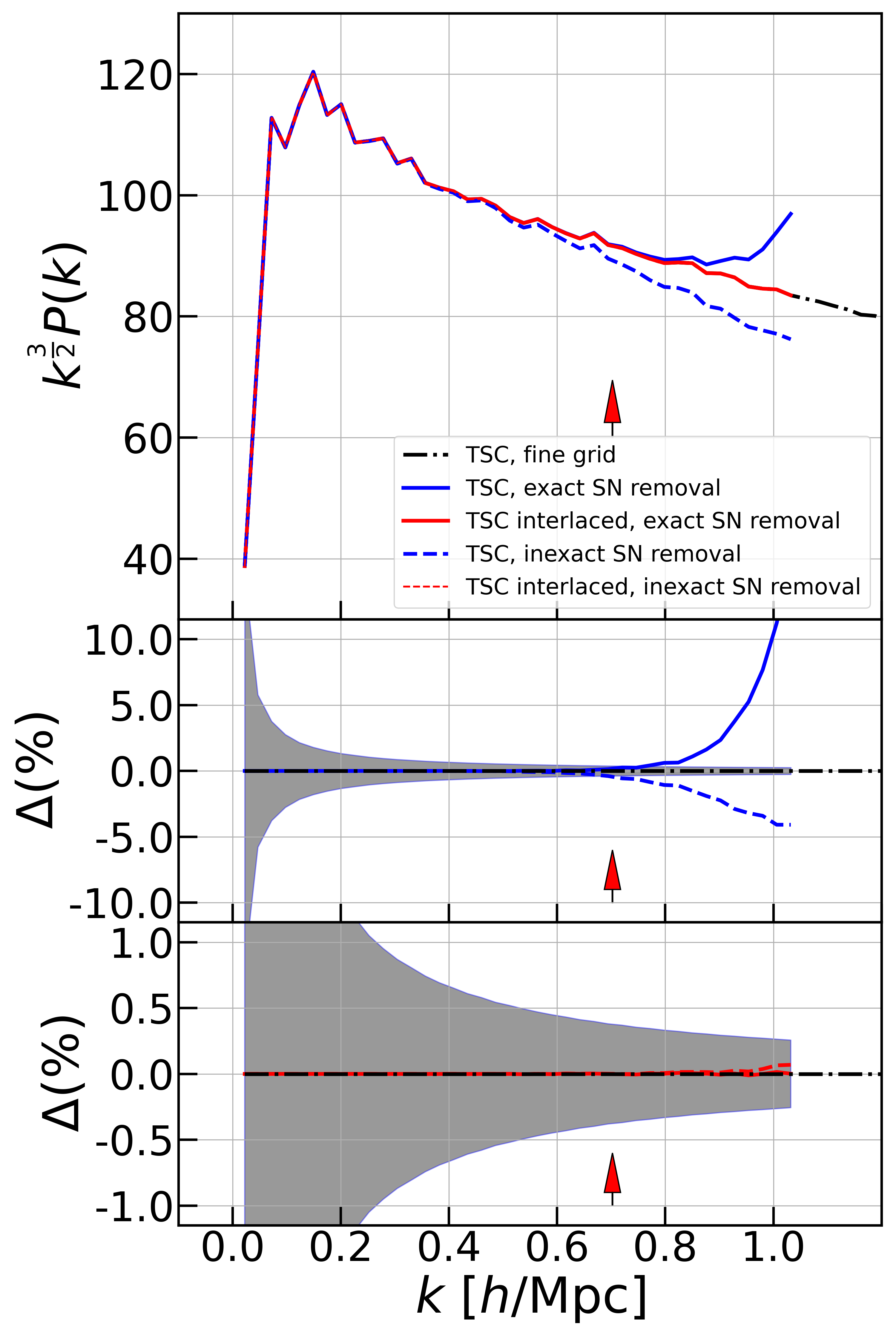
Figure 2: The power spectra of the full sample, with results for the CIC window function on the left and the TSC window function on the right. The top panel shows the power spectrum functions, while the middle and bottom panels depict the ratio of the power spectrum estimates to the results from the high-resolution grid. The blue lines represent the comparison between the two estimation methods without interlacing technique, and the red lines represent the comparison with interlacing technique. The dashed lines are calculated using the Nbodykit library, following the sequence of operations that involve correcting the window function first and then correcting the shot noise, according to the estimation formulae Eq. (2.10) and Eq. (2.17). Conversely, the solid lines follow Eq. (2.9) and Eq. (2.16). The red arrows in the graph indicate the frequency $k=\pi\sqrt[3]{n_{s}}$ that characterizes the sample’s average spatial separation. The gray region represents the statistical fluctuations of the power spectrum, i.e., $\pm\sigma=\pm\frac{P}{\sqrt{N_{\textrm{mode}}}}$, where $N_{\textrm{mode}}$ denotes the number of modes of each $k$ bin.

Based on the aforementioned samples, we test the results using the CIC and TSC window functions with a grid size of $N_{g}=200$. The mesh size is $3\,h^{-1}{\rm Mpc}$ and the corresponding Nyquist frequency $k_{N}=1.047\,h{\rm Mpc}^{-1}$. We choose this relatively large mesh size under the consideration that for Stage-IV surveys a cubic box covering the whole footprint may reach $(6\,h^{-1}{\rm Gpc})^{3}$ and the analysis in performed on $2000^{3}$ mesh. We compare the differences among the four estimators mentioned above. To reflect the magnitude of systematic biases for the samples, we treat the results from a 10 times higher sampling rate, $N_{g}=2000$, as the true values for the power spectrum. We have confirmed that, at this high sampling frequency, the power spectrum results from different estimators with different window functions are overlapping with each other below the Nyquist frequency of $N_{g}=200$ mesh. Therefore, we can consider it as the true value for a low sampling frequency result. For the full sample with a total count of $N_{s}=2,413,300$ and a number density of $n_{s}=1.12\times 10^{-2}\,h^{3}{\rm Mpc}^{-3}$ , the power spectrum results are shown in Figure 2.

Under the CIC window, Eq. (2.9) yields an overestimated result, with an error exceeding 10% at $k=k_{N}$. Eq. (2.10) gives an underestimated result, with an error of around 10% near $k=k_{N}$. Both errors far exceed the level of statistical fluctuations. However, with the interlacing technique, Eq. (2.17) exhibits errors larger than statistical fluctuations only at the scale of $k=0.9k_{N}$, reaching around 1% at $k=k_{N}$. Meanwhile, Eq. (2.16) maintains an error within 0.1%.

Under the TSC window, the errors are reduced. Eq. (2.9) provides an overestimated result, with an error of approximately 10% at $k=k_{N}$. Eq. (2.10) yields an underestimated result, with an error of around 5% near $k=k_{N}$. Both errors still significantly exceed the level of statistical fluctuations. However, with the interlacing technique, both Eq. (2.16) and Eq. (2.17) exhibit errors smaller than the level of statistical fluctuations within the Nyquist frequency. Specifically, Eq. (2.16) has an error within 0.002% at $k=k_{N}$, while Eq. (2.17) has an error within 0.1%.

We can observe that adopting higher-order window functions with the interlacing technique effectively reduces estimation errors, which is the main conclusion of [9]. However, when not using the interlacing technique, the reduction of errors with higher-order window functions is not significant. In terms of performance under the interlacing technique, Eq. (2.16) performs better than Eq. (2.17).

3.2 10% randomly selected halos

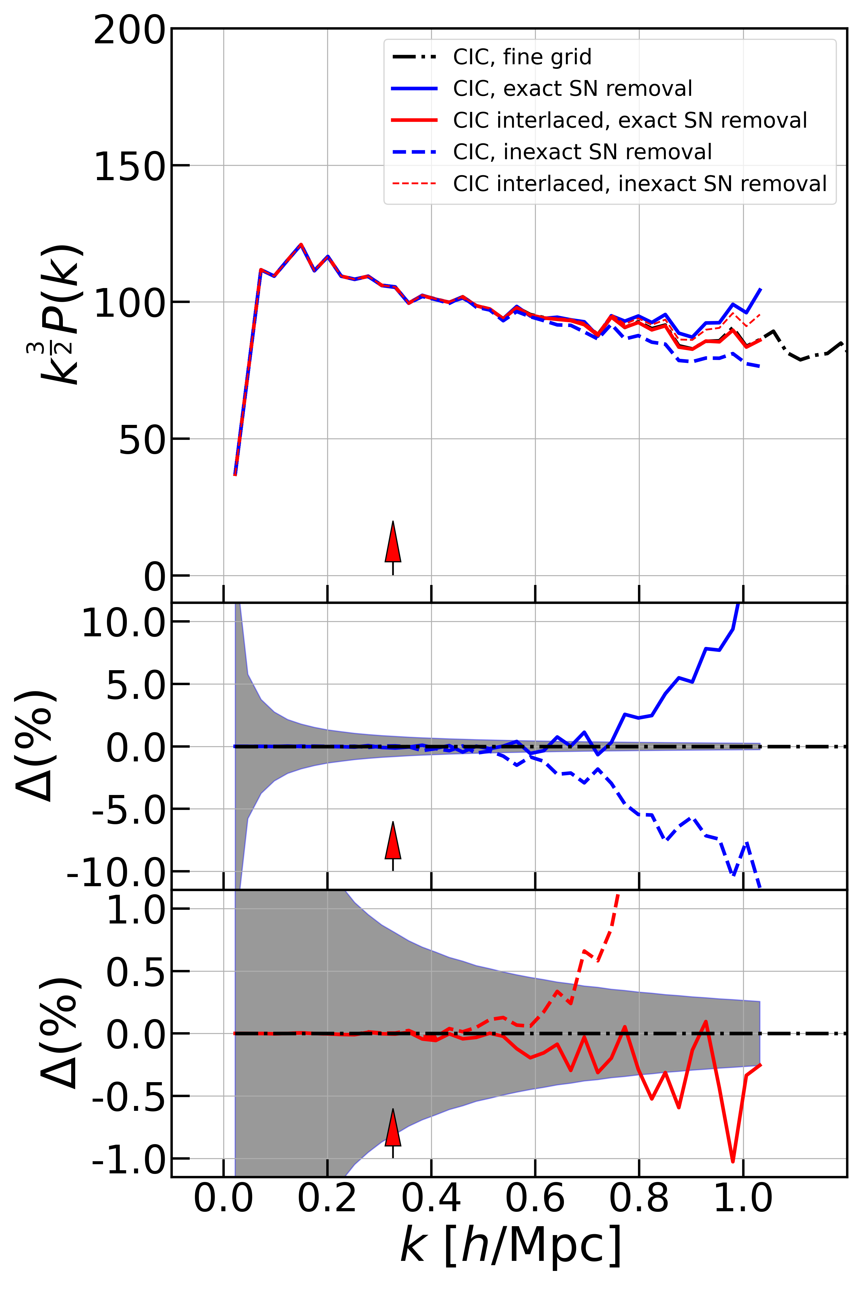
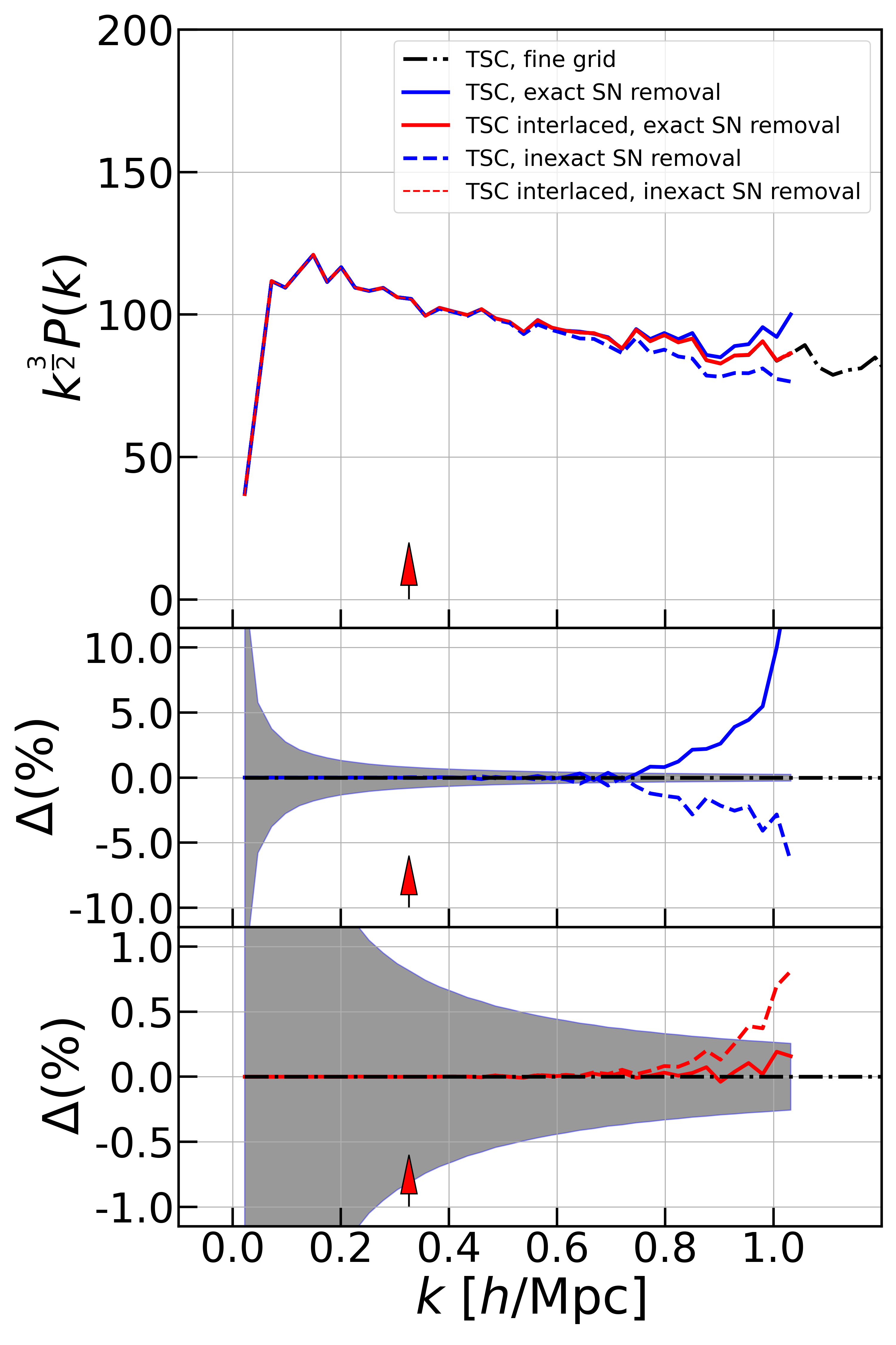
Figure 3: The power spectrum of the 10% randomly sampled data. The symbols have the same meaning as those in Figure 2.

We perform the same calculations as in Section 3.1, but this time we randomly selected 10% of the samples from the entire sample, resulting in a sample size of $N_{s}=241,330$. The sample number density is $n_{s}=1.12\times 10^{-3}\text{ Mpc}^{-3}h^{3}$. We obtain the power spectrum with the same amplitude as in Section 3.1, but the corresponding shot noise term $\frac{1}{N}$ is ten times larger after down-sampling, resulting in larger fluctuations on top of the original power spectrum. The results are shown in Figure 3.

Under the CIC window, Eq. (2.9) provides an overestimated result, and Eq. (2.10) yields an underestimated result. Both errors exceed 10% near $k=k_{N}$, far exceeding the level of statistical fluctuations. With the interlacing technique, Eq. (2.17) exhibits errors exceeding the level of statistical fluctuations below the scale of $k=0.7k_{N}$, reaching 10% at $k=k_{N}$, while Eq. (2.16) maintains an error within 1% despite larger fluctuations.

Under the TSC window, the errors are improved. Eq. (2.9) provides an overestimated result, with an error of approximately 10% at $k=k_{N}$. Eq. (2.10) yields an underestimated result, with an error of around 5% near $k=k_{N}$. Both errors still significantly exceed the level of statistical fluctuations. With the interlacing technique, Eq. (2.16) exhibits errors smaller than statistical fluctuations within the Nyquist frequency. Specifically, it has an error below 0.2% at $k=k_{N}$, while Eq. (2.17) exceeds the level of statistical fluctuations and reaches 0.7%.

Compared to the result in Section 3.1, the systematic bias is significantly larger due to the lower sample density, especially for the estimators with inexact shot noise subtraction. We can see that under the interlacing technique, the estimation Eq. (2.16) still performs better than Eq. (2.17).

3.3 10% high mass halos

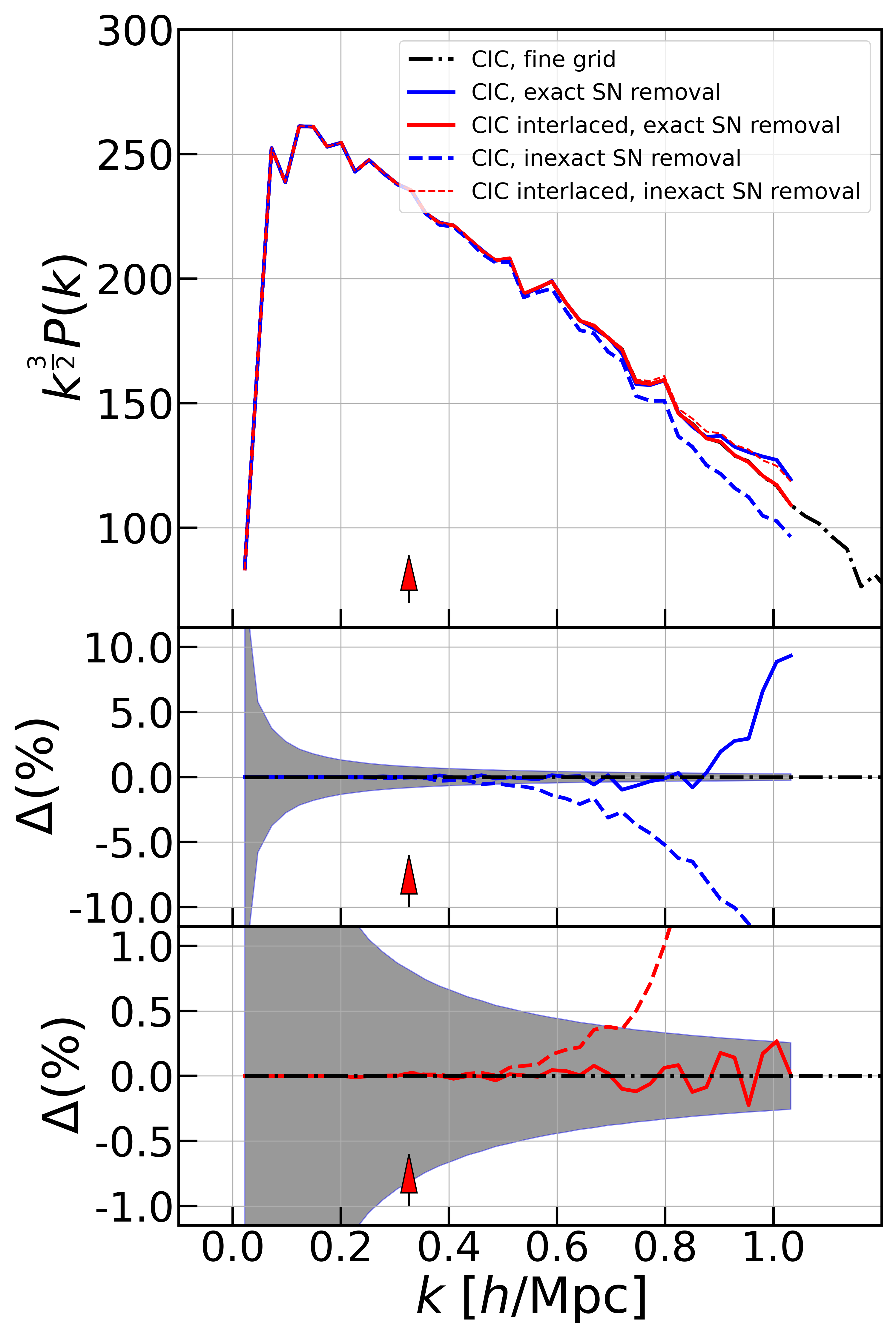
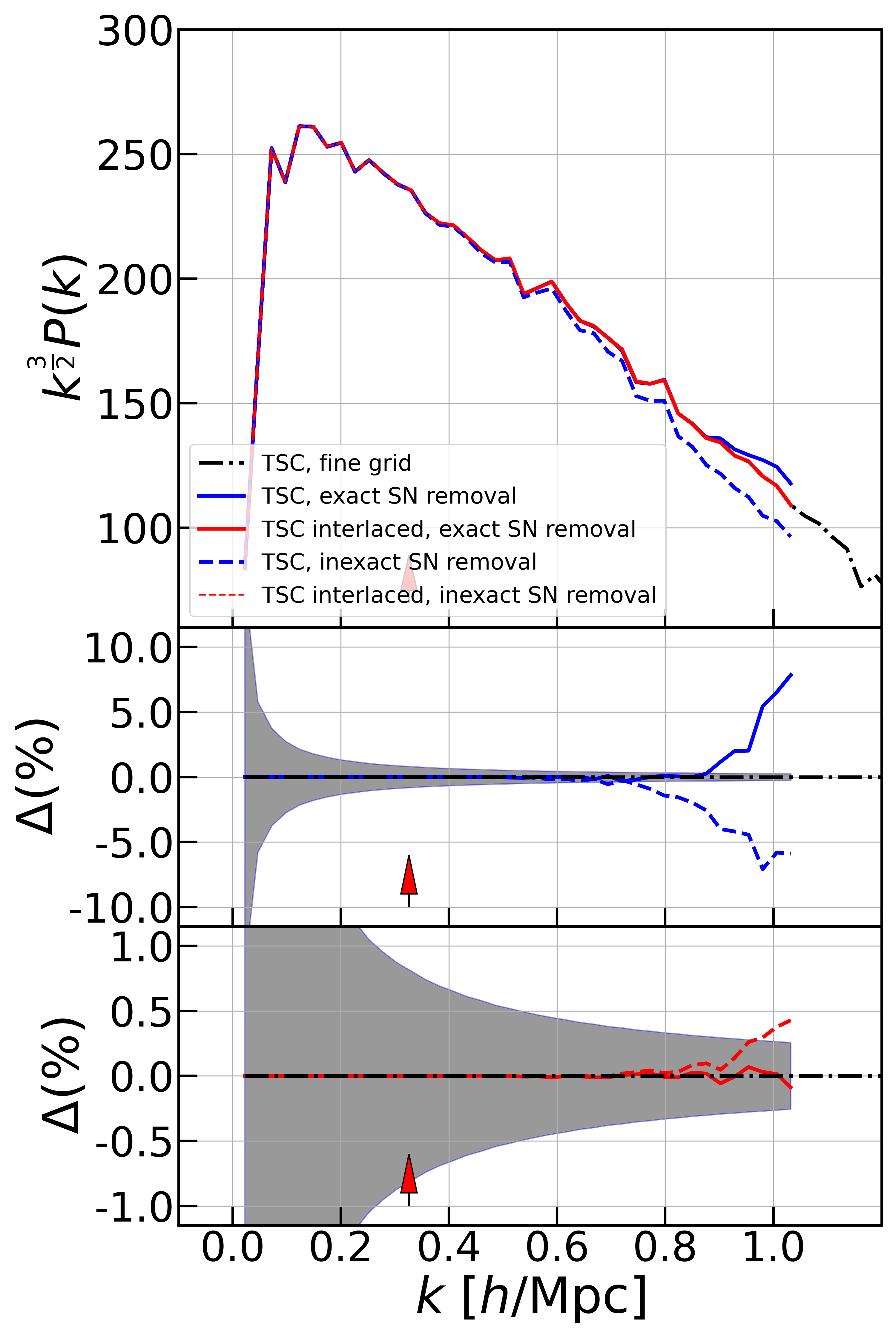
Figure 4: The power spectrum of a 10% subsample selected in high mass, with the same symbols as in Figure 2.

We perform the same calculations as in Section 3.1, but this time we select the top 10% of the samples in terms of mass from the entire sample, resulting in a sample size of $N_{s}=241,330$. The number density is $n_{s}=1.12\times 10^{-3}\text{ Mpc}^{-3}h^{3}$. High-mass halos tend to exhibit higher clustering than low-mass halos. Therefore, the power spectrum amplitudes are no longer the same as those obtained in Section 3.1. The large power spectrum amplitude of this sample makes the shot noise less important. However, the corresponding shot noise term $\frac{1}{N}$ unavoidably amplifies as the average number density decreases, resulting in larger fluctuations on top of the power spectrum. The results are shown in Figure 4.

Again, Eq. (2.9) provides an overestimated result, and Eq. (2.10) yields an underestimated result for CIC window. Both errors reach approximately 10% near $k=k_{N}$, far exceeding the level of statistical fluctuations. However, Eq. (2.9) still maintains an error of around 1% within $k=0.8k_{N}$, while Eq. (2.10) exceeds at larger scales. With the interlacing technique, Eq. (2.17) exhibits errors larger than statistical fluctuations below the scale of $k=0.7k_{N}$, reaching 9% at $k=k_{N}$. On the other hand, Eq. (2.16) fluctuates but remains within the level of statistical fluctuations. Under the TSC window, the errors are improved. Eq. (2.9) provides an overestimated result, with an error of approximately 7% at $k=k_{N}$. Eq. (2.10) yields an underestimated result, with an error of around 5% near $k=k_{N}$. Both errors still significantly exceed the level of statistical fluctuations. However, with the interlacing technique, Eq. (2.16) exhibits errors smaller than statistical fluctuations within the Nyquist frequency. Specifically, it has an error below 0.1% at $k=k_{N}$, while Eq. (2.17) exceeds statistical fluctuations only near the Nyquist frequency. We can see that under this sampling scheme, the estimation Eq. (2.16) still demonstrates superior accuracy.

3.4 1% randomly selected halos

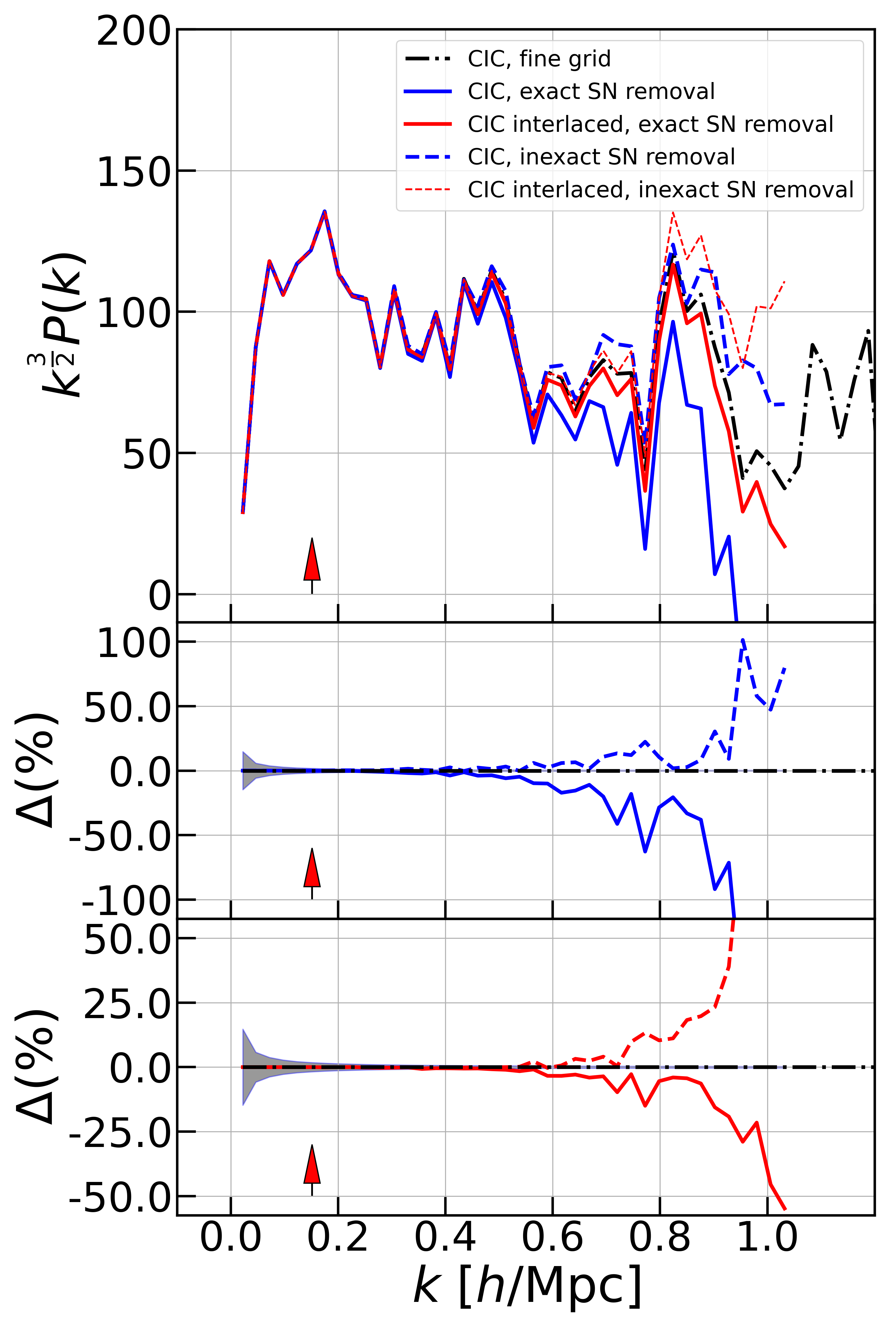
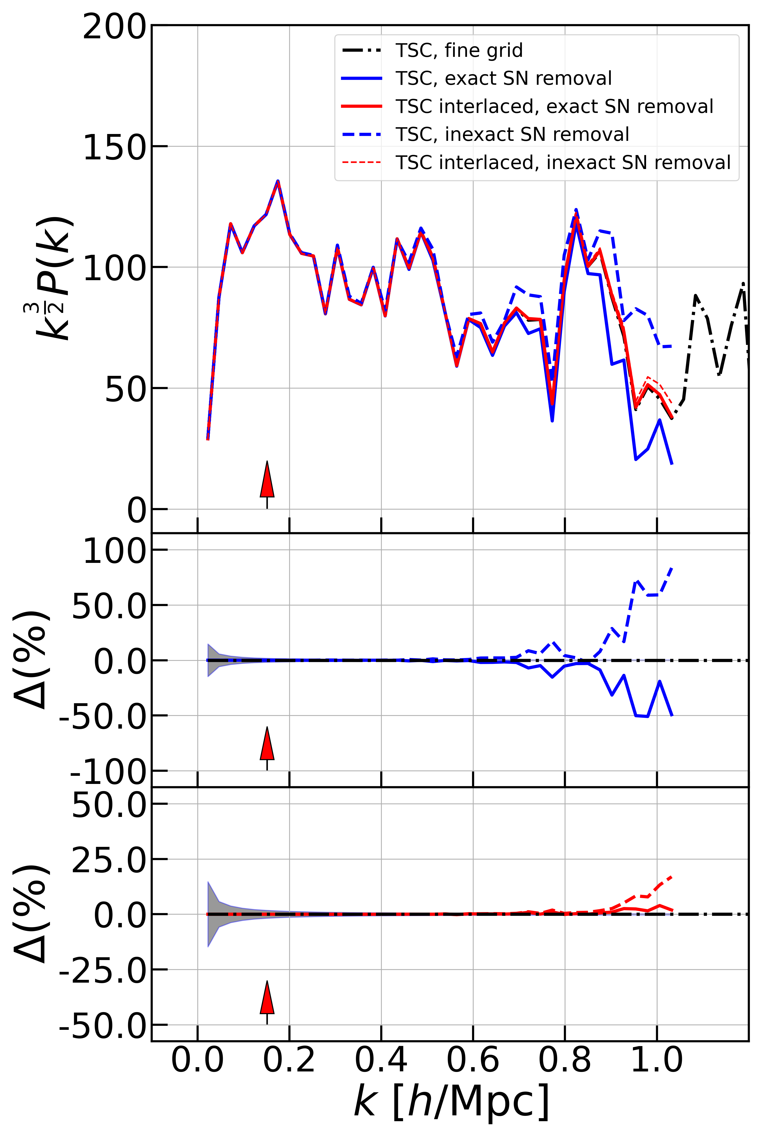
Figure 5: The power spectrum of the 1% randomly sampled data. The symbols have the same meaning as those in Figure 2.

We randomly select a sparse sample from the total dataset, consisting of 1% of the total sample size, which corresponds to $N_{s}=24,133$ halos. The number density of this sparse sample is $n_{s}=1.12\times 10^{-4}\,\text{Mpc}^{-3}h^{3}$. We perform the same computation as described in Section 3.1 on this sparse sample, and we expect to obtain power spectra with the same amplitude as in Section 3.1. However, due to the sparsity of this sample, the resulting power spectrum will exhibit even larger fluctuations compared to the results in Section 3.2. The results are presented in Figure 5. Under the CIC window, Eq. (2.10) overestimates the results, while Eq. (2.9) underestimates them. Both estimations show errors of around 10% near $k=0.7k_{N}$, which greatly exceeds the size of statistical fluctuations. Under the interlacing technique, Eq. (2.17) exhibits errors of over 50% at $k=0.9k_{N}$, while Eq. (2.16) exhibits errors of over 50% near the Nyquist frequency. Under the TSC window, Eq. (2.10) overestimates the results, with an error of over 50% at $k=0.95k_{N}$, and Eq. (2.9) underestimates them, with an error within 50% near the Nyquist frequency. Both estimations still greatly exceed the size of statistical fluctuations. Although under the interlacing technique the errors still exceed the size of statistical fluctuations. Eq. (2.16) exhibits errors within 5% near the Nyquist frequency, while Eq. (2.17) exhibits errors of around 15% near the same frequency. It can be seen that under this sampling scheme, the estimation using Eq. (2.16) still demonstrates a precision advantage.

3.5 1% high mass halos

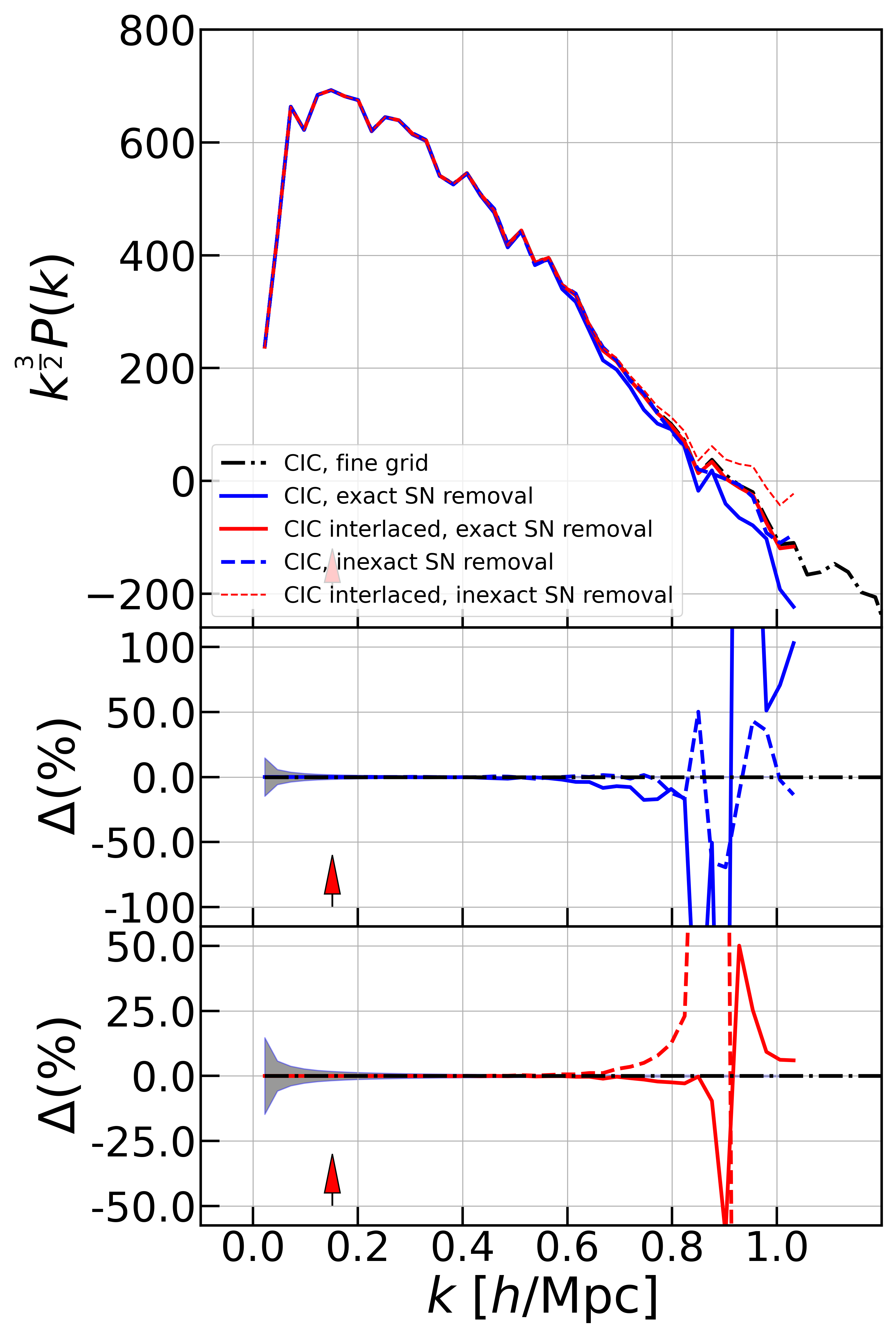
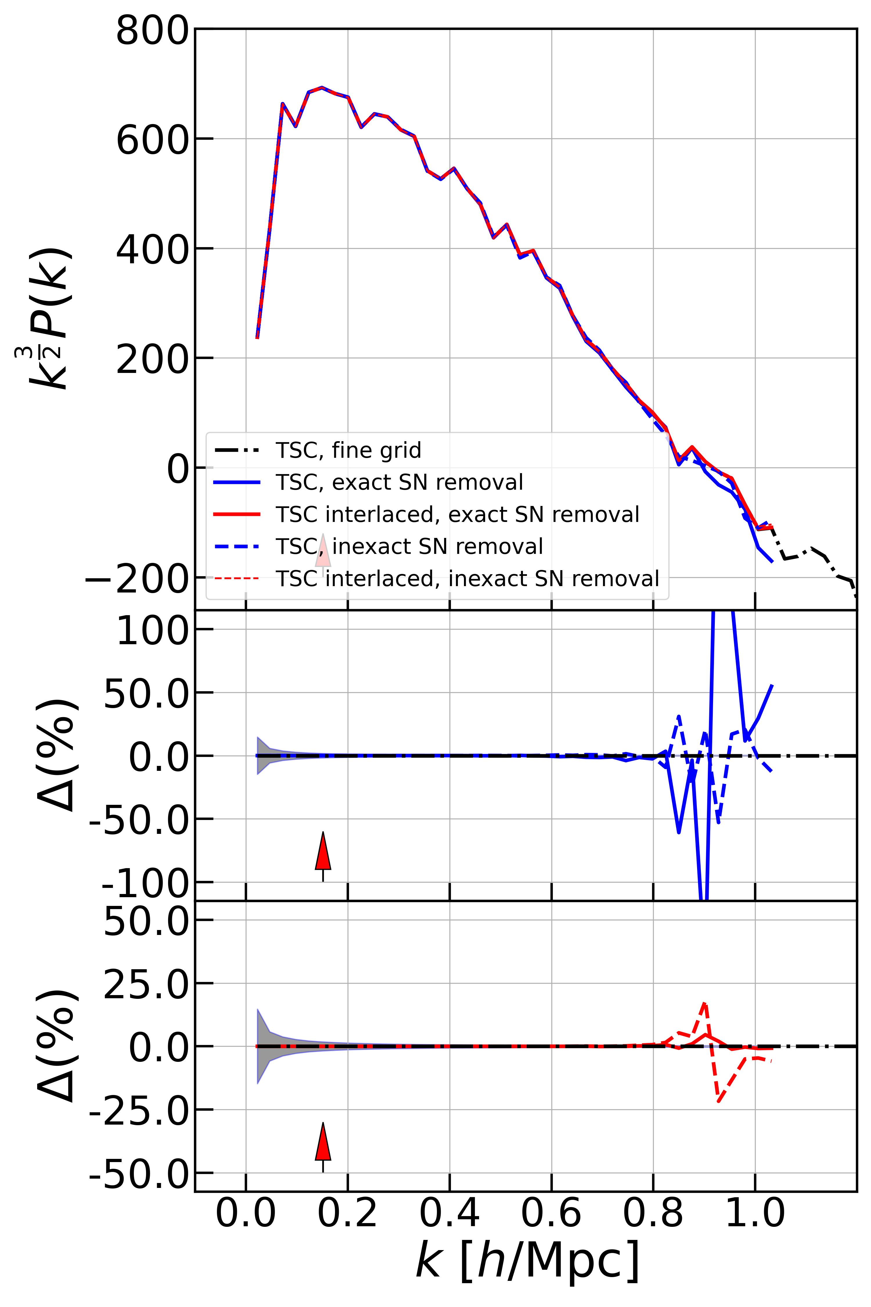
Figure 6: The power spectrum of a 1% subsample selected in high mass, with the same symbols as in Figure 2.

The power spectrum of the 1% top mass halos, with a total sample size of $N_{s}=24,133$ and a number density of $n_{s}=1.12\times 10^{-4}\,\text{Mpc}^{-3}h^{3}$, has been computed using the same configuration as the previous sections. The results are presented in Figure 6. The power spectrum exhibits a higher level of clustering due to the selection of high-mass components. However, the estimated power spectrum is less than zero in the small scale even the fine grid is adopted. This nonphysical result is due to the fact that the halo distribution for this sample is sub-Poissonian. For example, in [4], for the most massive halo bin, the shot noise is only at a level of $2/3$ of the expected $1/N$ value. Thus, our esitmators naively over-subtract the shot noise term by assuming the shot noise being $1/N$. Despite the nonphysical reason for the negative power in the calculation, the comparison of different estimators is still valid in the sense that they are compared to the fine grid result. But the zero-crossing in the fiducial power spectrum leads to large fluctuations in the ratio plot. As a result, the values near that point are sensitive to how the frequency approaches it, leading to a false oscillation in the power spectrum ratio. We prefer not to compare the values near the zero-crossing scale. Overall, in the case of the 1% high mass data, the power spectrum estimation using the interlacing technique with Eq. (2.16) still provides the best results.

4 Conclusion

In this article, we have presented four approaches for power spectrum calculation using FFT and compared their performance. It is widely known by the community that the shot noise is a constant $\frac{1}{N}$ as halo/galaxy distribution is Poissonian. Although this approximation is widely adopted in general estimations (as Eq. (2.10) and Eq. (2.17)), when using the interlacing technique, the aliasing effects on the signal term are reduced, and thus the impact of aliasing on the shot noise term can no longer be neglected. We have provided the specific form of the shot noise term under the interlacing technique in Eq. (2.15), which demonstrates how the shot noise term is affected by the window function and aliasing effects. We have also pointed out that Eq. (2.16) provides a better estimation compared to Eq. (2.17). In precise cosmological analysis, this algorithm allows for a more accurate subtraction of shot noise, helping to reduce the systematic bias induced by the detailed numerical calculation. This reduction of the systematics toward the Nyquist frequency also saves the computational cost, since for a good power spectrum estimator such as Eq. (2.16) we could use coarse mesh in the analysis for a given precision requirement on a specified scale. This is of great importance as the precise cosmological constraints rely on large suite of mock observation of order $\mathcal{O}(10^{4})$ to obtain the reasonably good covariance matrix [12]. Moreover, as realized in literature, the higher-order window functions yield better accuracy, particularly under the interlacing technique. Considering the increased computational cost associated with higher-order window functions, it is not recommended to increase the order of the window function without adopting the interlacing technique, as it does not effectively reduce systematic errors. Under similar consideration, using better estimator could save computational cost by only using low order window function.

We have made the code implementing Eq. (2.9) and Eq. (2.16) available at https://github.com/ColdThunder/FFTps.

Appendix A Isotropic Approximation for Shot Noise

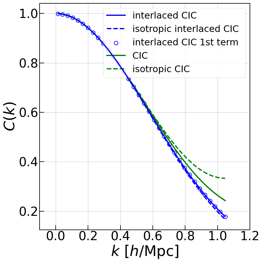
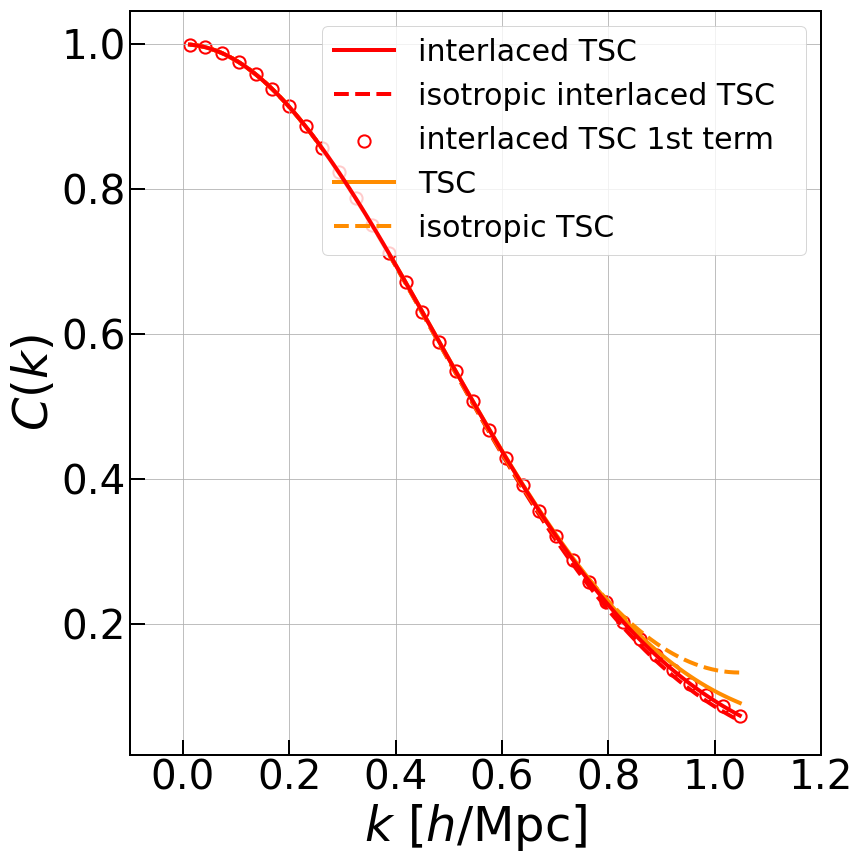
Figure 7: Analytical shot noise expressions are presented. On the left side are the results for the CIC window function, and on the right side are the results for the TSC window function. The dashed lines are the isotropic version following Eq. (A.2) for interlacing and Eq. (2.8) for non-interlacing. The solid lines are the exact calculation, following Eq. (2.15) and Eq. (A.1) for interlacing and non-interlacing, respectively. The scattered points are the first term in Eq. (2.15).

As in [7], the isotropic version for the shot noise without interlacing is

$$C^{\mathrm{iso}}(k)=\left\{\begin{aligned} &1\ ,&\text{NGP}\ ,\\ &1-\frac{2}{3}\sin^{2}\left(\frac{\pi k}{k_{H}}\right)\ ,&\text{CIC}\ ,\\ &1-\sin^{2}\left(\frac{\pi k}{k_{H}}\right)+\frac{2}{15}\sin^{4}\left(\frac{\pi k}{k_{H}}\right)\ ,&\text{TSC}\ ,\\ &1-\frac{4}{3}\sin^{2}\left(\frac{\pi k}{k_{H}}\right)+\frac{2}{5}\sin^{4}\left(\frac{\pi k}{k_{H}}\right)-\frac{4}{315}\sin^{6}\left(\frac{\pi k}{k_{H}}\right)\ ,&\text{PSC}\ .\\ \end{aligned}\right.$$ (A.1)

In short, it approximates $\prod_{i}S_{2p}[\sin^{2}(\pi k_{i}/k_{H})]$ as $S_{2p}[\sin^{2}(\pi k/k_{H})]$. For the case with interlacing, the exact anisotropic shot noise is Eq. (2.15). The similar approximation above can only be straightforwardly applied to the first term $\prod_{i}C_{e}(k_{i})$. We show that the first term is overwhelming in Figure 7. Keeping the first term only gives an relative error about 0.3% when approaching Nyquist frequency with CIC window function, and 0.02% with TSC window function.

Given that the above approximation is valid, it is straightforward to treat the isotropic version of the first term $\prod_{i}C_{e}(\pi k_{i}/2k_{H})\approx C_{e}(\pi k/2k_{H})$ as the isotropic approximation for interlacing.

$$C^{{\operatorname{int}},\mathrm{iso}}(k)=\left\{\begin{aligned} &\cos^{2}\left(\frac{\pi k}{2k_{H}}\right),&\text{NGP}\ ,\\ &\cos^{4}\left(\frac{\pi k}{2k_{H}}\right)\left[1-\frac{2}{3}\sin^{2}\left(\frac{\pi k}{2k_{H}}\right)\right]\ ,&\text{CIC}\ ,\\ &\cos^{6}\left(\frac{\pi k}{2k_{H}}\right)\left[1-\sin^{2}\left(\frac{\pi k}{2k_{H}}\right)+\frac{2}{15}\sin^{4}\left(\frac{\pi k}{2k_{H}}\right)\right]\ ,&\text{TSC}\ ,\\ &\cos^{8}\left(\frac{\pi k}{2k_{H}}\right)\left[1-\frac{4}{3}\sin^{2}\left(\frac{\pi k}{2k_{H}}\right)+\frac{2}{5}\sin^{4}\left(\frac{\pi k}{2k_{H}}\right)-\frac{4}{315}\sin^{6}\left(\frac{\pi k}{2k_{H}}\right)\right]\ ,&\text{PSC}\ .\\ \end{aligned}\right.$$ (A.2)

In short, $C^{{\operatorname{int}},{\mathrm{iso}}}(k)=\cos^{2p}(\pi k/2k_{H})C^{\mathrm{iso}}(k/2)$. Note that the prefactor of $\cos^{2p}x$ can be expressed as polynomial of $\sin^{2}x$ up to order $p$, leaving the whole formula only containing sine terms. Or we can express all the terms in the polynomial of $\sin^{2}x$ into polynomial of $\cos^{2}x$. However, these further expansions help less when we input the above formula using programming language. Thus we keep this mixed form of cosine and sine terms in $C^{{\operatorname{int}},{\mathrm{iso}}}(k)$. Also in Figure 7, the exact shot noise term is compared with the isotropic shot noise for both interlacing and non-interlacing case. The isotropic approximation for interlacing case is better than the one without interlacing.

Appendix B Shot Noise for High Order Interlacing

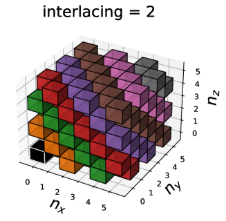
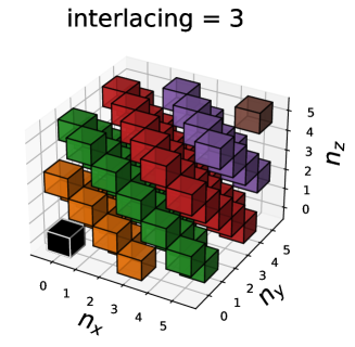
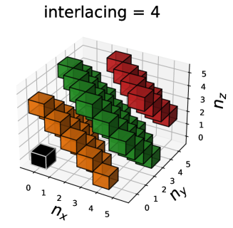
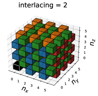
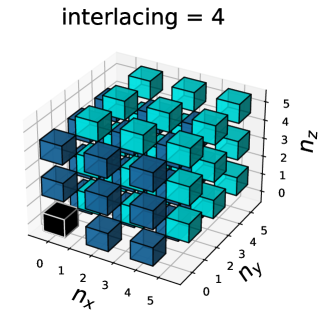
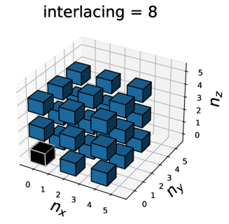
Figure 8: The interlacing schemes (residual images) in frequency space. The black voxel denotes the cardinal term with ${\boldsymbol{n}}=0$. The top panels represent the equal-spacing interlacing scheme with 2, 3 and 4 interlaced grids, and the bottom panels represent the bisection interlacing scheme with 2, 4 and 8 interlaced grids. In top panels, each color denotes a group of residual images in one plane. In bottom panels, each color denote a lattice structure that has an offset to the others.

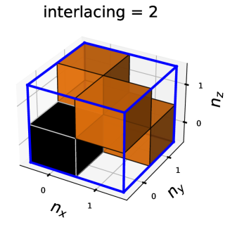
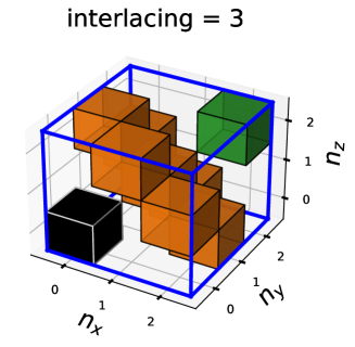
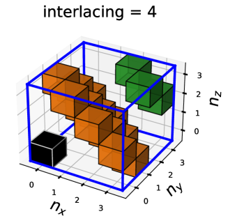
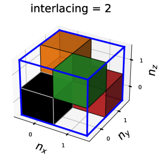
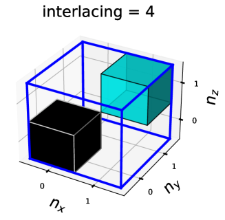
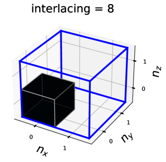
Figure 9: The repeating unit concatenating up in three dimension to make up of the residual images in frequency space in Figure 8. The infinite summation over each block in those units can be calculated individually as $C^{\operatorname{int-1D},n^{\prime}_{x}}_{m}(k_{x})C^{\operatorname{int-1D},n^{\prime}_{y}}_{m}(k_{y})C^{\operatorname{int-1D},n^{\prime}_{z}}_{m}(k_{z})$.

The main goal of interlacing technique is to eliminate aliased images. For 2 interlaced grids, the second mesh which has a shift $(H/2,H/2,H/2)$ relative to the primary one can eliminate the main aliasing contamination from $|{\boldsymbol{n}}|=1$. To eliminate more images, using more interlaced grids, i.e. high order interlacing, is useful. However, different high order schemes appear in literature. We list two of them.

• Equal-spacing interlacing scheme.

• Bisection interlacing scheme.

For the equal-spacing interlacing scheme, $m$ interlaced grids are adopted, which are placed at $(jH/m,jH/m,jH/m)$ for $j=0,1,\cdots,m-1$. This scheme was proposed by [1] (see also [6]), and used in pypower. For the bisection interlacing scheme, the high order interlaced grids are located at the middle of the low order ones. For 4 interlaced grids, the origin of the interlaced grids are located at $(0,0,0)$, $(0,H/2,H/2)$, $(H/2,0,H/2)$, $(H/2,H/2,0)$. For 8 interlaced grids, the positions are $(0,0,0)$, $(0,0,H/2)$, $(0,H/2,0)$, $(0,H/2,H/2)$, $(H/2,0,0)$, $(H/2,0,H/2)$, $(H/2,H/2,0)$, $(H/2,H/2,H/2)$. This scheme appeared in [8] (see also [6]).

The residual aliased images for the two schemes are presented in Figure 8. Here we directly comment on the two schemes from the sketch in the figure, and leaving the mathematical derivation later. For the equal-spacing scheme, the elimination seems to be efficient when $m\geq 3$. We caution that the plot is misleading since we put the $|{\boldsymbol{n}}|=0$ block in the corner. The residual images are distributed anisotropically, and all the images on $n_{x}+n_{y}+n_{z}=0$ plane is never eliminated for any order $m$. Thus, the main contamination is always from eight images at $(\pm 1,\mp 1,0)$, $(\pm 1,0,\mp 1)$ and $(0,\pm 1,\mp 1)$ even for $m\geq 3$. For bisection interlacing scheme with 4 interlaced grids, the main contamination is from the eight images that share the eight vertices of the primary one. While moving to 8 interlaced grids, all the images with distance less than 2, i.e. all the neighbour 26 images, are eliminated.

B.1 Equal-spacing interlacing scheme

Considering such an interlacing scheme that $m$ girds sequentially shift $(H/m,H/m,H/m)$ to the previous one, i.e. the $j$th grid ($j=2,3,\cdots,m$) is shifted from the first one by a distance of $((j-1)H/m,(j-1)H/m,(j-1)H/m)$ and produces a density field $\delta_{j}^{f}({\boldsymbol{k}})$. The arithmetic average of these samplings gives the interlaced denstiy field

$$\tilde{\delta}^{f}({\boldsymbol{k}}) =\frac{1}{m}\left[{\sum_{j=1}^{m}}\delta^{f}_{j}({\boldsymbol{k}})\right]$$ (B.1)

$$=\sum_{\boldsymbol{n}}{\theta_{\boldsymbol{n}}{\delta}^{f}({\boldsymbol{k}}+k_{H}{\boldsymbol{n}})}\ .$$

Similar to Eq. (2.12), $\theta_{\boldsymbol{n}}$ is defined as

$$\theta_{\boldsymbol{n}} \equiv\frac{1}{m}\left[{\sum_{j=1}^{m}}e^{-2\mathrm{i}\pi j(n_{x}+n_{y}+n_{z})/m}\right]$$ (B.2)

$$=\left\{\begin{array}[]{ll}1\ ,&(n_{x}+n_{y}+n_{z})/m\text{ is an integer}\ ,\\ 0\ ,&\text{ otherwise}\ .\end{array}\right.$$

Obviously, the residual images locate on planes with $n=n_{x}+n_{y}+n_{z}=ml$ and $l$ being any integer, as in the top panels in Figure 8.

To sum up the contributions from these anisotropically distributed aliased images, we first decompose the whole space into periodical patches along three Cartesian directions. Each patch contains same $m\times m$ voxels as shown in the top panels in Figure 9. Consequently, the contribution from these patches can be calculated separately for each dimension, and inside each patch we need to sum up the contributions from the residual images shown as colored blocks. Mathematically, this decomposition corresponds to expanding $\theta_{\boldsymbol{n}}$ as

$$\theta_{\boldsymbol{n}} \equiv\frac{1}{m}\left[{\sum_{j=1}^{m}}e^{-2\mathrm{i}\pi j(n_{x}+n_{y}+n_{z})/m}\right]$$ (B.3)

$$=\sum_{(n^{\prime}_{x},n^{\prime}_{y},n^{\prime}_{z})\in G}\left[\frac{1}{m}{\sum_{j=1}^{m}}e^{-2\mathrm{i}\pi j(n_{x}-n^{\prime}_{x})/m}\right]\left[\frac{1}{m}{\sum_{j=1}^{m}}e^{-2\mathrm{i}\pi j(n_{y}-n^{\prime}_{y})/m}\right]\left[\frac{1}{m}{\sum_{j=1}^{m}}e^{-2\mathrm{i}\pi j(n_{z}-n^{\prime}_{z})/m}\right]\ .$$

Here, $G$ is the group satisfying $n^{\prime}_{x}+n^{\prime}_{y}+n^{\prime}_{z}=0,m$ for $m=2$, and $n^{\prime}_{x}+n^{\prime}_{y}+n^{\prime}_{z}=0,m,2m$ for $m\geq 3$. $n^{\prime}_{x}$, $n^{\prime}_{y}$ and $n^{\prime}_{z}$ are integers in between $[0,m)$. The summation over group $G$ counts the contributions from all residual images in one patch. As shown in Figure 9, there are 4 blocks to count for $m=2$, 9 blocks for $m=3$, and 16 blocks for $m=4$. The summation over ${\boldsymbol{n}}$ in Eq. (B.1) collects the contributions over all patches.

In one dimension, the shot noise over images locating at $(0,\pm m,\pm 2m,\cdots)$ is

$$C^{\operatorname{int-1D}}_{m}(k) =|W(k)|^{2}\sum_{n=ml}\left(\frac{k}{k-nk_{H}}\right)^{2p}=|W(k)|^{2}\sum_{l}\left(\frac{k}{k-mlk_{H}}\right)^{2p}$$ (B.4)

$$=|W(k)|^{2}\sum_{l}\left(\frac{k/m}{k/m-lk_{H}}\right)^{2p}=\frac{|W(k)|^{2}}{|W(k/m)|^{2}}C(k/m)$$

$$=\frac{\sin^{2p}\left(\frac{\pi k}{k_{H}}\right)}{m^{2p}\sin^{2p}\left(\frac{\pi k}{mk_{H}}\right)}S_{2p}\left[\sin^{2}\left(\frac{\pi k}{mk_{H}}\right)\right]\ .$$

Straightforwardly, the summation over images locating at $(n_{\textrm{shift}},n_{\textrm{shift}}\pm m,n_{\textrm{shift}}\pm 2m,\cdots)$ is

$$C^{\operatorname{int-1D},n_{\textrm{shift}}}_{m}(k) =|W(k)|^{2}\sum_{l}\left(\frac{k}{k-(ml+n_{\textrm{shift}})k_{H}}\right)^{2p}$$ (B.5)

$$=\frac{\sin^{2p}\left(\frac{\pi k}{k_{H}}\right)}{m^{2p}\sin^{2p}\left(\frac{\pi k}{mk_{H}}-\frac{\pi n_{\textrm{shift}}}{m}\right)}S_{2p}\left[\sin^{2}\left(\frac{\pi k}{mk_{H}}-\frac{\pi n_{\textrm{shift}}}{m}\right)\right]\ .$$

Finally, the exact shot noise in this case is

$$C^{{\operatorname{int}}}_{m}({\boldsymbol{k}}) =\sum_{(n^{\prime}_{x},n^{\prime}_{y},n^{\prime}_{z})\in G}C^{\operatorname{int-1D},n^{\prime}_{x}}_{m}(k_{x})C^{\operatorname{int-1D},n^{\prime}_{y}}_{m}(k_{y})C^{\operatorname{int-1D},n^{\prime}_{z}}_{m}(k_{z})\ .$$ (B.6)

Note that group $G$ has 4 elements for $m=2$, i.e. $(n^{\prime}_{x},n^{\prime}_{y},n^{\prime}_{z})=(0,0,0)$, $(0,1,1)$, $(1,0,1)$ and $(1,1,0)$. This corresponds to the four terms in Eq. (2.15).

B.2 Bisection interlacing scheme

Obviously in Figure 8, the equal-spacing interlacing results in anisotropic residual image distribution for $m\geq 3$. In contrast, the bisection interlacing scheme prefers to eliminate the near images first. To eliminate the main aliased images with $|{\boldsymbol{n}}|=1$, two interlaced grids are adopted and as a byproduct $|{\boldsymbol{n}}|=\sqrt{3}$ images are also removed. To remove all $|{\boldsymbol{n}}|=1$ and $\sqrt{2}$ images, four interlaced grids are essential, but $|{\boldsymbol{n}}|=\sqrt{3}$ images will be left. To remove all $|{\boldsymbol{n}}|<2$ images, we have to increase the number of interlaced grids to 8. We caution that it is not cost-effective to remove only one more aliased image by doubling the computation cost from 4 interlaced grids to 8.

We list the $\theta_{\boldsymbol{n}}$ for using $m=1$ (i.e., no interlacing), $2$, $4$, $8$ and $16$ interlaced grids.

$$\theta_{\boldsymbol{n}} =\left\{\begin{aligned} \ &1,&\text{no interlace}\ ,\\ \ &\frac{1}{2}\left[1+{e^{-\pi\mathrm{i}n_{x}}}{e^{-\pi\mathrm{i}n_{y}}}{e^{-\pi\mathrm{i}n_{z}}}\right]\ ,&\text{2 interlaced}\ ,\\ &\frac{1}{4}\left[1+{e^{-\pi\mathrm{i}n_{x}}}{e^{-\pi\mathrm{i}n_{y}}}+{e^{-\pi\mathrm{i}n_{y}}}{e^{-\pi\mathrm{i}n_{z}}}+{e^{-\pi\mathrm{i}n_{z}}}{e^{-\pi\mathrm{i}n_{x}}}\right]\ ,&\text{4 interlaced}\ ,\\ \ &\frac{1}{8}\left[1+{e^{-\pi\mathrm{i}n_{x}}}\right]\left[1+{e^{-\pi\mathrm{i}n_{y}}}\right]\left[1+{e^{-\pi\mathrm{i}n_{z}}}\right],&\text{8 interlaced}\ ,\\ &\frac{1}{16}\left[1+{e^{-\frac{\pi\mathrm{i}n_{x}}{2}}}{e^{-\frac{\pi\mathrm{i}n_{y}}{2}}}{e^{-\frac{\pi\mathrm{i}n_{z}}{2}}}\right]\left[1+{e^{-\pi\mathrm{i}n_{x}}}\right]\left[1+{e^{-\pi\mathrm{i}n_{y}}}\right]\left[1+{e^{-\pi\mathrm{i}n_{z}}}\right]\ ,&\text{16 interlaced}\ ,\\ &\cdots,&\cdots\ .\end{aligned}\right.$$ (B.7)

In the expansion of $\theta_{n}$, there are exactly $m$ terms for $m$ interlaced grids. Each term takes the form $\frac{1}{m}e^{-2\pi\mathrm{i}\frac{H_{x}n_{x}+H_{y}n_{y}+H_{z}n_{z}}{H}}$, corresponding to an interlacing grid with offsets of $(H_{x},H_{y},H_{z})$, respectively. The residual images with $8m$ interlaced grids have the same pattern with $m$ interlaced case but the distance between residual images is scaled by a factor of two. Generalize to cases with $m=2^{3h}$, $2^{3h+1}$ or $2^{3h+2}$ ($h=0,1,\cdots$) interlaced grids,

$$\theta_{\boldsymbol{n}} =\left\{\begin{aligned} \ &\prod_{i=x,y,z}{\prod_{j=0}^{h}}\frac{1}{2}\left[1+{e^{-\frac{\pi\mathrm{i}n_{i}}{2^{j-1}}}}\right]\ ,&\text{$2^{3h}$ interlaced}\ ,\\ \ &\frac{1}{2}\left[1+\prod_{i=x,y,z}{e^{-\frac{\pi\mathrm{i}n_{i}}{2^{h}}}}\right]\prod_{i=x,y,z}{\prod_{j=0}^{h}}\frac{1}{2}\left[1+{e^{-\frac{\pi\mathrm{i}n_{i}}{2^{j-1}}}}\right]\ ,&\text{$2^{3h+1}$ interlaced}\ ,\\ \ &\frac{1}{4}\left[1+{e^{-\frac{\pi\mathrm{i}n_{x}}{2^{h}}}}{e^{-\frac{\pi\mathrm{i}n_{y}}{2^{h}}}}+\text{2 perms.}\right]\prod_{i=x,y,z}{\prod_{j=0}^{h}}\frac{1}{2}\left[1+{e^{-\frac{\pi\mathrm{i}n_{i}}{2^{j-1}}}}\right]\ ,&\text{$2^{3h+2}$ interlaced}\ .\end{aligned}\right.$$ (B.8)

The derivation of shot noise for $m=2^{3h}$ interlaced grids is straightforward because the summation of each direction can be done individually.

$$C^{\operatorname{int}}_{2^{3h}}({\boldsymbol{k}}) =W^{2}({\boldsymbol{k}})\frac{\sum_{{\boldsymbol{n}}}\theta_{\boldsymbol{n}}|W({\boldsymbol{k}}+k_{H}{\boldsymbol{n}})|^{2}}{W^{2}({\boldsymbol{k}})}$$ (B.9)

$$=W^{2}({\boldsymbol{k}})\prod_{i=x,y,z}\sum_{{\boldsymbol{n}}}{\prod_{j=1}^{h}}\frac{1}{2}\left[1+{e^{-\frac{\pi\mathrm{i}n_{i}}{2^{j-1}}}}\right]\left(\frac{k_{i}}{k_{i}-n_{i}k_{H}}\right)^{2p}$$

$$=\prod_{i=x,y,z}C^{\operatorname{int-1D}}_{2^{h}}(k_{i})\ .$$

It is simply the multiplication of three one dimensional shot noise expressions derived in Eq. (B.4) for $2^{h}$ interlaced grids.

In case of $m=2^{3h+1}$ interlacing, following the same strategy conducted in deriving Eq. (2.15), we can obtain the summation separately and individually. In one dimension, the residual images with $m=2^{h}$ interlaced grids are divided into odd terms and even terms, with $C_{m}^{{\operatorname{int}}}=C_{m}^{\operatorname{int-1D,odd}}+C_{m}^{\operatorname{int-1D,even}}$. Note that the even terms of $m=2^{(h-1)}$ interlacing are just the whole terms of $m=2^{h}$. Thus,

$$C^{\operatorname{int-1D,even}}_{2^{h}}(k)=C^{\operatorname{int-1D}}_{2^{h-1}}(k)\ .$$ (B.10)

For the odd terms, they have a shift with the even terms. Thus,

$$C^{\operatorname{int-1D,odd}}_{m=2^{h}}(k) =|W(k)|^{2}\sum_{n}\left(\frac{k}{k-(2^{h}n+2^{h-1})k_{H}}\right)^{2p}$$ (B.11)

$$=\frac{\sin^{2p}\left(\frac{\pi k}{k_{H}}\right)}{m^{2p}\cos^{2p}\left(\frac{\pi k}{mk_{H}}\right)}S_{2p}\left[\cos^{2}\left(\frac{\pi k}{mk_{H}}\right)\right]\ .$$

The odd terms can also be derived by considering the fact that the whole terms of $m$ interlacing are same as the even terms of $m-1$ interlacing. Thus,

$$C^{\operatorname{int-1D,odd}}_{2^{h}}(k)=C^{\operatorname{int-1D}}_{2^{h}}(k)-C^{\operatorname{int-1D,even}}_{2^{h}}(k)=C^{\operatorname{int-1D}}_{2^{h}}(k)-C^{\operatorname{int-1D}}_{2^{h-1}}(k)\ .$$ (B.12)

As such, the shot noise for $m=2^{3h+1}$ interlaced case can be written as

$$C^{\operatorname{int}}_{2^{3h+1}}({\boldsymbol{k}})=\prod_{i=x,y,z}C^{\operatorname{int-1D,even}}_{2^{h}}(k_{i})+\sum_{(i,j,l)\in A_{3}}C^{\operatorname{int-1D,even}}_{2^{h}}(k_{i})C^{\operatorname{int-1D,odd}}_{2^{h}}(k_{j})C^{\operatorname{int-1D,odd}}_{2^{h}}(k_{l})\ ,$$ (B.13)

which is consistent with Eq. (2.15) when $h=0$.

In case of $m=2^{3h+2}$, the summation reduces to two terms, i.e. all $n_{i}$’s are even and all $n_{i}$’s are odd, as shown in Figure 9. Therefore, the expression reads

$$C^{\operatorname{int}}_{2^{3h+2}}({\boldsymbol{k}}) =\prod_{i=x,y,z}C^{\operatorname{int-1D,even}}_{2^{h}}(k_{i})+\prod_{i=x,y,z}C^{\operatorname{int-1D,odd}}_{2^{h}}(k_{i})\ .$$ (B.14)

The last point worth mentioning is that $C_{8}^{\operatorname{int}}({\boldsymbol{k}})/W^{2}({\boldsymbol{k}})$ for 8 interlaced grids is exactly same as $C({\boldsymbol{k}})/W^{2}({\boldsymbol{k}})$ with no interlacing but doubling the resolution. In principle, at least for NGP, given the density fields on 8 interlaced grids, the density on two times finer grid can be solved out. This explains the above equivalence. The computational cost is roughly same, but the interlacing technique allows lower memory usage.

References

• Chen etΒ al., [1974] Chen, L., Bruce Langdon, A., and Birdsall, C. (1974). Reduction of the grid effects in simulation plasmas. Journal of Computational Physics, 14(2):200–222.
• Couchman, [1991] Couchman, H. (1991). Mesh-refined p3m-a fast adaptive n-body algorithm. The Astrophysical Journal, 368:L23–L26.
• Cui etΒ al., [2008] Cui, W., Liu, L., Yang, X., Wang, Y., Feng, L., and Springel, V. (2008). An Ideal Mass Assignment Scheme for Measuring the Power Spectrum with Fast Fourier Transforms. Astrophys. J., 687(2):738–744.
• Hamaus etΒ al., [2010] Hamaus, N., Seljak, U., Desjacques, V., Smith, R.Β E., and Baldauf, T. (2010). Minimizing the stochasticity of halos in large-scale structure surveys. Phys. Rev. D, 82(4):043515.
• Hand etΒ al., [2018] Hand, N., Feng, Y., Beutler, F., Li, Y., Modi, C., Seljak, U., and Slepian, Z. (2018). nbodykit: An Open-source, Massively Parallel Toolkit for Large-scale Structure. Astron. J., 156(4):160.
• Hockney and Eastwood, [2021] Hockney, R.Β W. and Eastwood, J.Β W. (2021). Computer simulation using particles. crc Press.
• Jing, [2005] Jing, Y.Β P. (2005). Correcting for the Alias Effect When Measuring the Power Spectrum Using a Fast Fourier Transform. Astrophys. J., 620:559–563.
• List etΒ al., [2023] List, F., Hahn, O., and Rampf, C. (2023). Fluid-limit Cosmological Simulations Starting from the Big Bang. arXiv e-prints, page arXiv:2309.10865.
• Sefusatti etΒ al., [2016] Sefusatti, E., Crocce, M., Scoccimarro, R., and Couchman, H.Β M.Β P. (2016). Accurate estimators of correlation functions in Fourier space. Mon. Not. Roy. Astron. Soc., 460(4):3624–3636.
• Springel etΒ al., [2022] Springel, V., Pakmor, R., Zier, O., and Reinecke, M. (2022). GADGET-4: Parallel cosmological N-body and SPH code. page ascl:2204.014.
• Yang etΒ al., [2009] Yang, Y.-B., Feng, L.-L., Pan, J., and Yang, X.-H. (2009). An optimal method for the power spectrum measurement. Research in Astronomy and Astrophysics, 9(2):227–236.
• Yu etΒ al., [2016] Yu, Y., Zhang, P., and Jing, Y. (2016). Fast generation of weak lensing maps by the inverse-gaussianization method. Physical Review D, 94(8).