REAL: Representation Enhanced Analytic Learning for Exemplar-free Class-incremental Learning

Abstract

Exemplar-free class-incremental learning (EFCIL) aims to mitigate catastrophic forgetting in class-incremental learning without available historical data. Compared with its counterpart (replay-based CIL) that stores historical samples, the EFCIL suffers more from forgetting issues under the exemplar-free constraint. In this paper, inspired by the recently developed analytic learning (AL) based CIL, we propose a representation enhanced analytic learning (REAL) for EFCIL. The REAL constructs a dual-stream base pretraining (DS-BPT) and a representation enhancing distillation (RED) process to enhance the representation of the extractor. The DS-BPT pretrains model in streams of both supervised learning and self-supervised contrastive learning (SSCL) for base knowledge extraction. The RED process distills the supervised knowledge to the SSCL pretrained backbone and facilitates a subsequent AL-basd CIL that converts the CIL to a recursive least-square problem. Our method addresses the issue of insufficient discriminability in representations of unseen data caused by a frozen backbone in the existing AL-based CIL. Empirical results on various datasets including CIFAR-100, ImageNet-100 and ImageNet-1k, demonstrate that our REAL outperforms the state-of-the-arts in EFCIL, and achieves comparable or even more superior performance compared with the replay-based methods.

1 Introduction

Class-incremental learning (CIL) [15, 22] allows models to acquire knowledge from separately arriving data in a phase-by-phase manner. The CIL gains popularity for its ability to continuously adapt trained networks to unseen data. This manner emphasizes that specific data categories may be limited to certain locations or time slots and enables models to learn without resource-intensive joint retraining. Also, it resembles the human learning process that continuously gains new information from existing knowledge. Hence, the development of the CIL contributes to the accumulation of machine intelligence.

While class-incremental learning (CIL) offers several benefits, it is plagued by the issue of catastrophic forgetting [1], where models rapidly lose previously learned knowledge when acquiring new information. To mitigate the forgetting issue, various solutions have been proposed. Among these solutions, replay-based techniques have shown competitive results via storing historical samples but introduce privacy risks. As their counterpart, the exemplar-free CIL (EFCIL) does not save previous data to address the privacy issue but experiences severer forgetting problem without exemplars.

Among the EFCIL techniques, regularization-based methods have emerged as the first effective solutions. They reduce catastrophic forgetting by imposing constraints that prevent changes in important weights or activations. However, this inhibits models from learning from new tasks while restricting the modification of certain parameters. Recently, a new branch of CIL named analytic learning (AL) based CIL [34] has shown promising results while adhering to the exemplar-free constraint.

The AL-based CIL introduces a recursive paradigm where a linear classifier is trained incrementally phase by phase. This paradigm offers a weight-invariant property, meaning that weights trained recursively in each phase are identical to those trained on the entire data simultaneously [34, 35]. By first incorporating this property into the CIL, the ACIL [34] achieves highly competitive results. Additionally, the recursive operation enables the AL-based CIL to achieve strong performance particularly in large-phase scenarios (e.g., 50-phase).

However, existing AL-based methods freeze their feature extractors after the base phase, resulting in insufficient discriminability of representations for unseen data categories. The analytic classifiers trained in AL-based CIL are linear classifiers that highly rely on the separable features. Their classification performances can be essentially limited by the presence of less separable representations. This limitation has motivated the exploration of potential approaches to enhance the ability of backbone to extract representations.

Recently, self-supervised contrastive learning (SSCL) [11] has gained prominence for its effective transfer to downstream tasks. It learns general representations through contrastive proxy tasks without labels and the learned general representations can be effectively adapted to downstream tasks, showcasing the potential for knowledge transfer to the paradigm of CIL where the model is initially trained on a base phase and then incrementally learns new tasks. On the other hand, the knowledge distillation [9] (KD) adapts a student model to a teacher model by combining the knowledge of both labels and the understanding of data distribution from the teacher model. This hybrid knowledge effectively enhances knowledge transfer [28].

In this paper, we propose the Representation Enhanced Analytic Learning (REAL) for EFCIL. Inspired by the aganda similarity between the SSCL and CIL, and the knowledge transfer potential of KD, the REAL seeks to enhance the backbone’s ability to extract discriminate representations for unseen categories via pretraining and adaptation. Structurally, a dual-stream base pretraining (DS-BPT) for backbones is conducted during the base phase to obtain general knowledge. A representation enhancing distillation (RED) process follows, which collaboratively infuses the knowledge of labels to further enhance the pretrained model. The REAL advances the AL-based CIL family by enhancing the extraction of representations without sacrificing the basic benefits (i.e., weight-invariant property). The key contributions are summarized as follows.

$\bullet$ We present the REAL, an exemplar-free technique that provides improved representation extraction and analytical solution to the CIL problem.

$\bullet$ The DS-BPT pretrains backbones in two streams of both supervised learning and SSCL. The SSCL stream facilitates the learning of general representations without labels while the supervised learning stream trains a model to incorporate label information in the subsequent agenda.

$\bullet$ The RED process transfers label information to the SSCL pretrained backbone, allowing the backbone to further enhance the representation while preserving general knowledge. Hence, our REAL is expected to provide more discriminate representations during CIL.

$\bullet$ Experiments on benchmark datasets demonstrate that the REAL outperforms existing EFCIL methods including AL-based techniques, and even surpasses most replay-based methods.

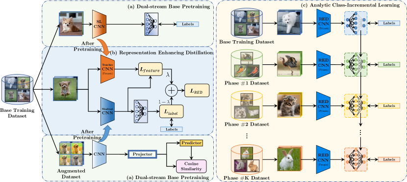
Figure 1: The REAL starts with the training on base phase, consisting of (a) Dual-stream base pretraining (DS-BPT) and (b) representation enhancing distillation (RED) on the base training dataset, followed by (c) analytic class-incremental learning. The CNN networks are first pretrained with two streams of supervised learning and self-supervised contrastive learning (SSCL) for obtaining the base knowledge (i.e., in (a)). The teacher CNN pretrained with supervised learning transfers knowledge to the student CNN pretrained with SSCL via the RED process (i.e., in (b)). The CIL of REAL is conducted by obtaining LS solutions recursively with an analytic classifier (i.e., in (c)).

2 Related Works

In this section, we provide a comprehensive review of CIL techniques covering both replay-based and EFCIL methods. We also discuss techniques closely related to the proposed REAL, e.g., the SSCL and the KD.

2.1 Replay-based CIL

Replay-based CIL, as first introduced by iCaRL [22], reinforces models’ memory by replaying historical data. Such a replay mechanism has gained popularity with various attempts following. The LUCIR [10] replaces the softmax layer with a cosine one. The PODNet [4] implements an efficient spatial-based distillation loss to reduce forgetting. The FOSTER [26] employs a two-stage learning paradigm, expanding and then reducing the network to the original size. The AANets [18] integrates a stable block and a plastic block to balance stability and plasticity. The RMM [19] leverages reinforcement learning to dynamically manage memory for exemplars. The online hyperparameter optimization [20] adaptively optimizes the stability-plasticity balance without prior knowledge.

2.2 Exemplar-free CIL

The EFCIL methods address the privacy concerns and mitigate catastrophic forgetting without exemplars. The EFCIL can be roughly categorized into regularization-based CIL, prototype-based CIL, and the recently proposed analytic learning (AL) based CIL.

The regularization-based CIL imposes additional constraints on network activations or weights to mitigate forgetting. The LFL [12] penalizes the activation difference. The LwF [15] prevents activation changes between old and new networks. The EWC [13] captures prior importance using a diagonally approximated Fisher information matrix. Building upon the EWC, [16] seeks a more appropriate replace of Fisher information matrix.

The prototype-based CIL mitigates forgetting by storing prototypes to avoid overlapping representations of new and old classes. For instances, the PASS [31] augments the prototypes to distinguish previous classes. The SSRE [32] introduces a prototype selection mechanism. The Fetril [21] reduces forgetting by generating pseudo-features of old classes from new representations.

The AL-based CIL is a recent developed branch of EFCIL that aims to find closed-form solutions on all seen data. The analytic learning (AL) [6, 33] is a technique that utilizes least squares (LS) to yield closed-form solutions during the training of neural networks. The ACIL [34] first introduces AL to the CIL realm. It is developed by reformulating the CIL procedure into a recursive LS form and equalize the CIL to joint training in the linear classifier. The subsequent GKEAL [35] is specialized in few-shot CIL settings by adopting a Gaussian kernel process that excels in data-scarce scenarios. The AL-based CIL exhibits strong performance. [34]. However, it relies on a frozen backbone trained solely on the base dataset, which may result in less-effective representations during CIL. In this paper, we overcome this limitation by introducing the REAL.

2.3 Self-supervised Contrastive Learning

The SSCL [11] enables label-free learning via a contrastive manner. It encourages feature convergence for similar samples and divergence for dissimilar ones. For instance, SimCLR [2] utilizes a symmetric Siamese network for contrastive training. MOCO [8] mitigates the influence of extreme samples through momentum updates. BYOL [5] introduces auxiliary structures for an asymmetric network trained with momentum. Built upon the BYOL, SimSiam [3] replaces the momentum mechanism with gradient stopping. The models trained by SSCL learn to extract general representations and can be effectively transferred [17].

2.4 Knowledge Distillation

The KD [9] is a technique that transfers knowledge from a teacher model to a student model. Common approaches include mimicking the student model’s output probabilities or feature representations to those of teacher model. The vanilla KD [9] uses the output probabilities to train the networks. The FitNets [23] transfers knowledge through intermediate features and attention maps are used in [29]. The FSP [27] model the teacher model’s inference process to provide the clues.

3 The Proposed Method

In this section, details of the proposed REAL are presented. The REAL focuses on representation enhancing which contains a DS-BPT and a RED process at the base phase. Subsequently, the analytic class-incremental agenda conducts the CIL in a recursive least-square form. An overview of REAL is depicted in Figure 1.

3.1 Representation Enhancing

Prior to further description, some definitions related to the CIL are presented. Suppose that the CIL asks for a $K$-phase learning. At each phase (e.g., phase $k$), training data of disjoint classes $\mathcal{D}_{k}^{\text{train}}\sim\{\bm{X}_{k}^{\text{train}},\bm{Y}_{k}^{\text{train}}\}$ ($k=1,\dots,K$) are available, where $\bm{X}_{k}^{\text{train}}\in\mathbb{R}^{N_{k}\times c\times w\times h}$ (e.g., images with the shape of $c\times w\times h$ ) and $\bm{Y}_{k}^{\text{train}}\in\mathbb{R}^{N_{k}\times d_{y_{k}}}$ (with phase $k$ including $d_{y_{k}}$ classes) are stacked $N_{k}$-sample input and label (one-hot) tensors. The objective of CIL at phase $k$ is to train networks given $\mathcal{D}_{k}^{\text{train}}$ and test them on $\mathcal{D}_{0:k}^{\text{test}}$ (with $\mathcal{D}_{k}^{\text{test}}\sim\{\bm{X}_{k}^{\text{test}},\bm{Y}_{k}^{\text{test}}\}$ ). Specifically, $\mathcal{D}_{0}^{\text{train}}\sim\{\bm{X}_{0}^{\text{train}},\bm{Y}_{0}^{\text{train}}\}$ represents the base training set and $\mathcal{D}_{0:k}$ indicates the joint dataset from phase $0$ to phase $k$.

Dual-stream Base Pretraining. The network is first pretrained in streams of supervised learning and SSCL to obtain the base knowledge during base phase before a subsequent enhancement. The stream of SSCL produces a backbone with general base knowledge detached from the labels, and the stream of supervised learning trains a backbone to acquire representations under supervision. The process of DS-BPT is shown in Figure 1 (a). In this paper, we adopt the SimSiam [3] as the SSCL architecture, which comprises a Siamese network of CNN backbone and formulates contrastive proxy tasks between different views (i.e. different augmentations of the same image).

Auxiliary structures, namely projector and predictor, are incorporated to assist SSCL training as extra mappings. For input $\bm{X}^{\text{train}}_{0}$, suppose that the random data augmentation operation is denoted as $f_{\text{RA}}$, the two views can be represented as $\bm{X}^{\text{aug}_{1}}=f_{\text{RA}}(\bm{X}^{\text{train}}_{0})$ and $\bm{X}^{\text{aug}_{2}}=f_{\text{RA}}(\bm{X}^{\text{train}}_{0})$. Let $\bm{W}_{\text{proj}}$, $\bm{W}_{\text{pred}}$ and $\bm{W}_{\text{CNN}}^{\text{SSCL}}$ represent the weights of the projector, predictor and the CNN backbone. Given two views ($\bm{X}^{\text{aug}_{1}}$, $\bm{X}^{\text{aug}_{2}}$) of input $\bm{X}\in\mathbb{R}^{c\times w\times h}$, the outputs are,

$$\bm{X}^{\text{proj}_{1}} =f_{\text{proj}}(f_{\text{flat}}(f_{\text{CNN}}(\bm{X}^{\text{aug}_{1}},\bm{W}_{\text{CNN}}^{\text{SSCL}})\bm{W}_{\text{proj}}))$$ (1)

$$\bm{X}^{\text{proj}_{2}} =f_{\text{proj}}(f_{\text{flat}}(f_{\text{CNN}}(\bm{X}^{\text{aug}_{2}},\bm{W}_{\text{CNN}}^{\text{SSCL}})\bm{W}_{\text{proj}}))$$ (2)

$$\bm{X}^{\text{pred}_{1}} =f_{\text{pred}}(\bm{X}^{\text{proj}_{1}},\bm{W}_{\text{pred}})$$ (3)

$$\bm{X}^{\text{pred}_{2}} =f_{\text{pred}}(\bm{X}^{\text{proj}_{2}},\bm{W}_{\text{pred}})$$ (4)

where $f_{\text{CNN}}$ indicates passing through the CNN backbone, $f_{\text{flat}}$ is a flattening operator, $f_{\text{proj}}$ and $f_{\text{pred}}$ are operations of projector and predictor respectively.

Then we optimize the negative cosine similarity of representations. For two tensors $\bm{Z}_{1}$, $\bm{Z}_{2}\in\mathbb{R}^{N\times d}$, the negative cosine similarity can be defined as

$$\bm{L}_{\text{cos}}(\bm{Z}_{1},\bm{Z}_{2})=-\sum_{i=1}^{N}\frac{\bm{z}_{1,i}\cdot\bm{z}_{2,i}}{\left\lVert\bm{z}_{1,i}\right\rVert_{2}{\left\lVert\bm{z}_{2,i}\right\rVert_{2}}}$$ (5)

where $\bm{z}_{j,i}$ is a row vector of $\bm{Z}_{j}$ ($i=1,2,\dots,N$; $j=1,2$), $\cdot$ is dot product operation and $\lVert\cdot\rVert_{2}$ is L2-norm. The loss function of SSCL can be

(6)

and we can use the BP algorithm to minimize $\bm{L}_{\text{SSCL}}$ to get a finely trained model in the SSCL stream.

For the stream of supervised learning, suppose that $\bm{W}_{\text{CNN}}^{\text{SL}}$ and $\bm{W}^{\text{SL}}_{\text{FCN}}$ are the weights of CNN backbone and fully connected network (FCN), the output can be

$$\bm{\hat{Y}}^{\text{SL}}=f_{\text{softmax}}(f_{\text{flat}}(f_{\text{CNN}}(\bm{X}_{0}^{\text{train}},\bm{W}_{\text{CNN}}^{\text{SL}}))\bm{W}_{\text{FCN}}^{\text{SL}}).$$ (7)

With labels $\bm{Y}_{0}^{\text{train}}$, we can train the model by BP algorithm with the loss function of cross entropy.

Representation Enhancing Distillation. After the pretraining of SSCL, the backbone acquires general base knowledge. In addition to the general knowledge, knowledge under supervision can serve as a valuable complement especially when conducting CIL in a supervised manner. We can further adapt the backbone to CIL tasks with extra supervised knowledge infused. We propose the RED process to adapt SSCL pretrained model to the subsequent CIL by introducing the complementary information of supervision.

Here, we employ the KD [9] to enhance the representation by transferring supervised knowledge through the extracted embeddings. These embeddings can be treated as features or representations encompassing the model’s understanding of the data distribution and can be calculated as

$$\bm{X}^{\text{SSCL}}=f_{\text{flat}}(f_{\text{CNN}}(\bm{X}^{\text{train}}_{0},\bm{W}_{\text{CNN}}^{\text{SSCL}}))$$ (8)

$$\bm{X}^{\text{SL}}=f_{\text{flat}}(f_{\text{CNN}}(\bm{X}^{\text{train}}_{0},\bm{W}_{\text{CNN}}^{\text{SL}})).$$ (9)

To transfer the understanding of data distribution under supervision, we mimic the embeddings extracted by the SSCL model to those of the model pretrained through supervised learning. We accomplish this by minimizing the difference between the features extracted from the two models with the metric of cosine similarity . Specifically, we aim to minimize the loss as follow. That is,

$$\bm{L}_{\text{feature}}=-\frac{1}{N}\sum_{i=1}^{N}\frac{\bm{x}^{\text{SL}}_{i}\cdot\bm{x}^{\text{SSCL}}_{i}}{\left\lVert\bm{x}^{\text{SL}}_{i}\right\rVert_{2}\left\lVert\bm{x}^{\text{SSCL}}_{i}\right\rVert_{2}}$$ (10)

where $\bm{x}^{\text{SL}}$ and $\bm{x}^{\text{SSCL}}$ are row vectors of $\bm{X}^{\text{SL}}$ and $\bm{X}^{\text{SSCL}}$.

Another source knowledge for representation enhancing comes from the labels themselves. In this approach, we can finetune the backbone in a supervised manner, leveraging the guidance provided directly by labels. To associate the representations extracted by the backbones with the labels, we insert a linear classifier after the backbone. The output of the model after this insertion is defined as

$$\leavevmode\resizebox{208.67871pt}{}{$\bm{\hat{Y}}^{\text{SSCL}}=f_{\text{softmax}}(f_{\text{flat}}(f_{\text{CNN}}(\bm{X}_{0}^{\text{train}},\bm{W}_{\text{CNN}}^{\text{SSCL}}))\bm{W}_{\text{FCN}}^{\text{SSCL}})$}.$$ (11)

The cross-entropy loss can be used to train the model with the knowledge source of labels, i.e.,

$$\bm{L}_{\text{label}}=-\frac{1}{N}\sum_{i=1}^{N}\log{\bm{\hat{y}}^{\text{SSCL}}_{i}}\bm{y}_{0,i}^{\text{train}}$$ (12)

where $\bm{\hat{y}}^{\text{SSCL}}$ and $\bm{y}_{0,i}^{\text{train}}$ are row vectors of $\bm{\hat{Y}}^{\text{SSCL}}$ and $\bm{Y}_{0}^{\text{train}}$. Finally, we can have the loss of representation enhancing

$$\bm{L}_{\text{RED}}=\lambda\bm{L}_{\text{feature}}+(1-\lambda)\bm{L}_{\text{label}}$$ (13)

where $\lambda$ is the parameter for balancing the contribution of teacher model and labels. After the RED, the trained CNN backbone is frozen in the following steps as the ACIL does.

Importance of Two Knowledge Sources in RED. The RED aims to enhance the SSCL backbone by incorporating supervised information as complementary knowledge. Relying solely on labels leads to direct adaptation to base phase labels, which can be easily forgotten during subsequent learning. Depending solely on the feature distribution from a teacher model might not be sufficiently effective, as the teacher model can potentially mislead the student model. Therefore, a combination of both knowledge sources is necessary and this pattern is evidenced in the ablation study.

3.2 Analytic Class-incremental Learning

Analytic Initialization. After the representation enhancing on the base dataset, our REAL seeks to further adapt the backbone to the following analytic CIL process by attaching previous backbone with an analytic classifier. The analytic classifier is a 2-layer network containing a buffer layer and a FCN. The buffer layer is to bridge the data distribution of BP training and analytic learning. There are a few choices [34][35] for the buffer layer. A convenient choice is a random initialized linear mapping, i.e. $f_{\text{buffer}}(\bm{X}_{0}^{(\text{cnn})})=\bm{X}_{0}^{(\text{cnn})}\bm{W}_{B}$. In this paper, we follow the ACIL to use a randomly initialized linear layer.

Here, an analytic initialization (AInit) process is required for initializing the weight of FCN at base phase. The first step of AInit is to obtain the embedding $\bm{X}_{0}^{\text{(cnn)}}\in\mathbb{R}^{N_{0}\times d_{\text{cnn}}}$ after the CNN backbone of input $\bm{X}^{\text{train}}_{0}$. Subsequently, the embedding is fed to the buffer layer to obtain mapped embedding $\bm{X}_{0}^{\text{(B)}}$, i.e.,

$$\bm{X}_{0}^{\text{(B)}}=f_{\text{Buffer}}(\bm{X}_{0}^{\text{(cnn)}})=f_{\text{Buffer}}(f_{\text{flat}}(f_{\text{CNN}}(\bm{X}_{0}^{\text{train}})))$$ (14)

where $f_{\text{Buffer}}$ indicates the operation of buffer. Next, we can optimize the FCN layer at base phase as the AInit via optimizing the following equation

$$\underset{\bm{W}_{\text{A}}}{\text{argmin}}\quad\left\lVert\bm{Y}_{0}^{\text{train}}-\bm{X}_{0}^{\text{(B)}}\bm{W}_{\text{A}}^{(0)}\right\rVert_{\text{F}}^{2}+{\gamma}\left\lVert\bm{W}_{\text{A}}^{(0)}\right\rVert_{\text{F}}^{2}$$ (15)

where $\lVert\cdot\rVert_{\text{F}}^{2}$ is Frobenius-norm, $\gamma$ is the regularization factor and $\bm{W}_{\text{A}}^{(0)}$ is the weight of FCN layer at the base phase. The optimal solution of equation 15 is

$$\bm{\hat{W}}_{\text{A}}^{(0)}=(\bm{X}_{0}^{\text{(B)T}}\bm{X}_{0}^{\text{(B)}}+\gamma\bm{I})^{-1}\bm{X}_{0}^{\text{(B)T}}\bm{Y}_{0}^{\text{train}}$$ (16)

where $\bm{\hat{W}}_{\text{A}}^{(0)}$ indicates the estimated weight of the FCN layer at phase 0, and $\cdot^{\text{T}}$ is the matrix transpose operator.

Class-incremental Learning. Upon completing the AInit process, the CIL begins. Let

where the sparse structure of $\bm{Y}_{0:k}^{\text{train}}$ is due to the disjoint tasks at each phase, and $\bm{X}_{i}^{\text{(B)}}$ is the $i^{\text{th}}$ representation

$$\bm{X}_{i}^{\text{(B)}}=f_{\text{Buffer}}(f_{\text{flat}}(f_{\text{CNN}}(\bm{X}_{i}^{\text{train}}))).$$ (17)

At phase k, the learning problem of all seen data $\mathcal{D}_{0:k}^{\text{train}}$ can be extended from (15) to

$$\leavevmode\resizebox{368.57964pt}{}{$\underset{\bm{W}_{\text{A}}^{(k)}}{\text{argmin}}\quad\left\lVert\bm{Y}_{0:k}^{\text{train}}-\bm{X}_{0:k}^{\text{B}}\bm{W}_{\text{A}}^{(k)}\right\rVert_{\text{F}}^{2}+{\gamma}\left\lVert\bm{W}_{\text{A}}^{(k)}\right\rVert_{\text{F}}^{2}$}.$$ (18)

The solution of (18) is

$$\leavevmode\resizebox{346.89731pt}{}{$\bm{\hat{W}}_{\text{A}}^{(k)}=(\bm{X}_{0:k}^{\text{(B)T}}\bm{X}_{0:k}^{\text{(B)}}+\gamma\bm{I})^{-1}\bm{X}_{0:k}^{\text{(B)T}}\bm{Y}_{0:k}^{\text{train}}$}.$$ (19)

The goal for CIL is to learn new tasks on $\mathcal{D}_{k}^{\text{train}}$ sequentially given a network trained on $\mathcal{D}_{0:k-1}^{\text{train}}$. However, in (19), we still need the previous data. To alleviate the reliance on previous data, let $\bm{R}_{k}=(\bm{X}_{0:k}^{\text{(B)T}}\bm{X}_{0:k}^{\text{(B)}}+\gamma\bm{I})^{-1}$ be the Autocorrelation Memory Matrix (AMM), the problem of requiring previous data can be solved in the following Theorem.

Theorem 3.1.

Let $\bm{\hat{W}}_{\text{A}}^{(k-1)\prime}=[\bm{\hat{W}}_{\text{A}}^{(k-1)}\ \ \ \bm{0}]$ be the optimal estimation of $\bm{\hat{W}}_{\text{A}}^{(k)}$ using (19) with all the training data from phase $0$ to $k$, is equivalent to

(20)

where

(21)

Proof.

See Supplementary material A. ∎

Theorem 3.1 indicates the results of joint training in (18) can be reproduced by recursively training on $\mathcal{D}_{k}^{\text{train}}$ sequentially. This implies the property that the CIL is equalized to joint training with both present and historical data. As shown in (20), the solution mainly consists of two parts: the addition observes new knowledge (i.e., $\bm{R}_{k}\bm{X}_{k}^{\text{(B)T}}\bm{Y}_{k}^{\text{train}}$), while the subtraction (i.e., $\bm{R}_{k}\bm{X}_{k}^{\text{(B)T}}\bm{X}_{k}^{\text{(B)T}}\bm{\hat{W}}_{\text{A}}^{(k-1)}$ ) corrects old categories because new knowledge would inevitably affect the old one (forget a small part of the old information to make room for the new one). This pattern ensures the requirement of preserving learned knowledge (stability) and accepting new information (plasticity) in CIL.

How Representation Enhancing Improves AL-based CIL? Existing AL-based methods face a major challenge of limited representations due to the frozen backbone. The backbone trained through supervised learning, fails to capture highly separable representations of categories learned outside the base phase, thereby limiting the effectiveness of linear classifiers. The proposed representation enhancing incorporates general representations from SSCL and information under supervision. The general representations capture primary separable features of categories during CIL and the RED provides further enhancement with supervised knowledge. Despite still freezing the backbone, our REAL provides more discriminate representations, facilitating the classification during the CIL process.

Table 1: Comparison of average accuracy $\mathcal{\bar{A}}$ and last-phase accuracy $\mathcal{A}_{K}$ among EFCIL and replay-based methods. Results from replay-based methods are cited from their papers. On CIFAR-100, data in (bracket) is for ResNet-32. Data in Bold are the best within EFCIL methods and data underlined are the best considering both categories. Data with “*” are those we reproduce via official codes. “-” means the results with corresponding setting are not available.

Metric	Method	Examplar-free?	CIFAR-100					ImageNet-100					ImageNet-1k
			K=5	10	25	50		K=5	10	25	50		K=5	10	25	50
$\mathcal{\bar{A}}$(%)	LUCIR (CVPR 2019)	$\times$	(63.17)	(60.14)	(57.54)	-		70.84	68.32	61.44	-		64.45	61.57	56.56	-
	PODNet (ECCV 2020)	$\times$	(64.83)	(63.19)	(60.72)	(57.98)		75.54	74.33	68.31	62.48		66.95	64.13	59.17	-
	POD+AANets (CVPR 2021)	$\times$	(66.31)	(64.31)	(62.31)	-		76.96	75.58	71.78	-		67.73	64.85	61.78	-
	POD+AANets+RMM (NeurIPS 2021)	$\times$	(68.36)	(66.67)	(64.12)	-		79.50	78.11	75.01	-		69.21	67.45	63.93	-
	FOSTER (ECCV 2022)	$\times$	-	67.95	63.83	-		-	77.54	69.34	-		-	-	-	-
	LwF (TPAMI 2018)	$\checkmark$	(49.59)	(46.98)	(45.51)	-		53.62	47.64	44.32	-		51.50	46.89	43.14	-
	ACIL (NeurIPS 2022)	$\checkmark$	(66.30)	(66.07)	(65.95)	(66.01)		74.81	74.76	74.59	74.13		65.34	64.84	64.63	64.35
	PASS (CVPR2021)	$\checkmark$	63.88*	60.07*	56.86*	41.11*		72.24*	67.97*	52.02*	30.59*		-	-	-	-
	IL2A (NeurIPS2021)	$\checkmark$	65.53*	60.51*	53.15*	21.49*		-	-	-	-		-	-	-	-
	FeTrIL (WACV2023)	$\checkmark$	66.30	65.20	-	-		72.20	71.20	-	-		66.10	65.00	-	-
	PRAKA (ICCV2023)	$\checkmark$	68.59*	68.51*	62.98*	43.09*		63.66*	62.75*	58.86*	41.24*		-	-	-	-
	REAL (ResNet-32)	$\checkmark$	(67.97)	(67.83)	(67.86)	(67.80)		-	-	-	-		-	-	-	-
	REAL (ResNet-18)	$\checkmark$	71.88	71.58	71.31	71.25		77.19	76.94	76.80	76.62		67.32	66.97	66.81	66.96
$\mathcal{A}_{K}$(%)	LUCIR (CVPR 2019)	$\times$	(54.30)	(50.30)	(48.35)	-		60.00	57.10	49.26	-		56.60	51.70	46.23	-
	PODNet (ECCV 2020)	$\times$	(54.60)	(53.00)	(51.40)	-		67.60	65.00	55.34	-		58.90	55.70	50.51	-
	POD+AANets (CVPR 2021)	$\times$	(59.39)	(57.37)	(53.55)	-		69.40	67.47	63.69	-		60.84	57.22	53.21	-
	POD+AANets+RMM (NeurIPS 2021)	$\times$	(59.00)	(59.03)	(56.50)	-		73.80	71.40	68.84	-		62.50	60.10	55.50	-
	LwF (TPAMI 2018)	$\checkmark$	(43.36)	(43.58)	(41.66)	-		55.32	57.00	55.12	-		48.70	47.94	49.84	-
	ACIL (NeurIPS 2022)	$\checkmark$	(57.78)	(57.79)	(57.65)	(57.83)		66.98	67.42	67.16	67.22		56.11	55.43	55.43	56.09
	PASS (CVPR2021)	$\checkmark$	55.75*	49.13*	44.76*	28.02*		61.76*	57.38*	37.46*	18.22*		-	-	-	-
	IL2A (NeurIPS2021)	$\checkmark$	53.36*	44.49*	35.27*	11.03*		-	-	-	-		-	-	-	-
	PRAKA (ICCV2023)	$\checkmark$	61.52*	60.12*	51.15*	27.14*		55.77*	54.77*	46.49*	21.80*		-	-	-	-
	REAL (ResNet-32)	$\checkmark$	(60.28)	(60.04)	(60.03)	(60.05)		-	-	-	-		-	-	-	-
	REAL (ResNet-18)	$\checkmark$	64.50	64.61	64.52	64.56		68.90	68.96	68.91	69.14		57.97	57.86	57.92	57.84

4 Experiments

In this section, experiments on various benchmark datasets are done to compare the REAL with SOTA EFCIL methods, including LwF [15], PASS [31], IL2A [30], ACIL [34], FeTrIL [21] and PRAKA [25]. We also include replay-based methods, i.e., LUCIR [10], PODNet [4], AANets [18], RMM [19] and FOSTER [26] as counterpart.

4.1 Experimental Setup

Datasets. We evaluate the performance of our REAL by on CIFAR-100 [14], ImageNet-100 [4] and ImageNet-1k [24]. For CIL evaluation, dataset is partitioned into a base training set (i.e., phase #0) and a sequence of incremental sets. The base dataset contains half of the full data classes. The network is first trained on the base dataset. Subsequently, the network gradually learns the remaining classes evenly for $K$ phases. In the experiment, we report the results for phase $K=5,10,25$ and $50$.

Implementation Details. The architecture in the experiment is ResNet-18 [7]. Additionally, we train a ResNet-32 on CIFAR-100 as many CIL methods (e.g. [34] and [19]) adopt this structure. We adopt the same training strategies for SSCL in [3]. For hyperparameters shared among AL-based methods, we copy them from the ACIL [34]. We further study on the hyperparameters in RED including the balancing parameter $\lambda$ and number of epochs $e$ for distillation. The implementation details of parameters can be found in Supplementary material B.

Evaluation Protocol. Two metrics are adopted for evaluation. The overall performance is evaluated by the average incremental accuracy (or average accuracy) $\mathcal{\bar{A}}$ (%): $\mathcal{\bar{A}}=\frac{1}{K+1}{\sum}_{k=0}^{K}\mathcal{A}_{k}$, where $\mathcal{A}_{k}$ indicates the average test accuracy at phase $k$ by testing the network on $\mathcal{D}_{0:k}^{\text{test}}$. A higher $\mathcal{\bar{A}}$ score is preferred when evaluating CIL algorithms. The other metric is the last-phase accuracy $\mathcal{A}_{K}$ (%) measuring the network’s last-phase performance after completing all CIL tasks. $\mathcal{A}_{K}$ (%) is an important metric as it reveals the gap between the CIL and the joint training, a gap all CIL methods stride to close.

4.2 Comparison with State-of-the-arts

We compare our REAL with both EFCIL and reply-based methods as demonstrated in Table 1. The upper panel shows the average accuracy $\mathcal{\bar{A}}$ and the lower panel shows the last-phase accuracy $\mathcal{A}_{K}$. Also, the phase-wise accuracy is plotted in Figure 2. The hyperparameters of $(\lambda,e)$ are $(0.4,20),(0.8,20)$ and $(0.9,40)$ on CIFAR-100, ImageNet-100 and ImageNet-1k respectively.

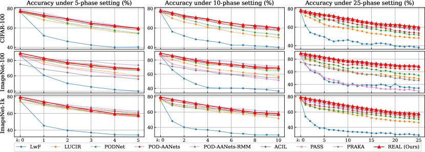
Figure 2: The phase-wise accuracy of compared methods on benchmark datasets with the $K=5,10,25$. The dash lines are the curves for replay-based methods.

Compare with EFCIL Methods. As shown in the upper panel in Table 1, the REAL delivers the most competitive results among the EFCIL methods. On CIFAR-100, the REAL leads at both $\mathcal{\bar{A}}$ and $\mathcal{A}_{K}$ with a significant extent in different phase settings. In particular, the performance of AL-based CIL (e.g., REAL and ACIL) remains roughly the same as $K$ changes, while other techniques receive degrading performance. This allows our REAL to excel more significantly for a growing $K$. On ImageNet-100, the $\mathcal{\bar{A}}$ achieves 77.19%, 76.94%, 76.80% and 76.62%, overtaking the previous best EFCIL by 2.38%, 2.18%, 2.21% and 2.49% respectively. The REAL’s last-phase accuracy yields 68.90%, 68.96%, 68.82% and 69.14%, leading the ACIL by 1.54%-1.92% among various $K$ scenarios. Similar patterns are demonstrated in the results of ImageNet-1k, showing that the REAL produces a significant improvement. From Figure 2, it can be intuitively found that our REAL exhibits strong performance compared with the EFCIL methods.

Compare with Replay-based Methods. Replay-based methods leverage historical samples during CIL and provide an effective solution to address catastrophic forgetting. As shown in Table 1, for small-phase scenarios (e.g., $K$ = 5, 10), the REAL performs slightly behind its replay-based counterparts. For instance, the REAL gives 77.19% averagely on ImageNet-100, underperforming the 79.50% from the “PODNet+AANets+RMM” combo. However, advantages of replaying past samples are consumed as $K$ increases. For instance, for 25-phase CIL on ImageNet-1k, the REAL leads the best replaying method by 2.88% (66.81% v.s. 63.93%) averagely, and by 2.42% (57.92% v.s. 55.50%) at the last phase. This pattern on ImageNet-1k is consistent with that on ImageNet-100. In general, the REAL begins to surpass replay-based methods from $K\geq 25$, except the $\mathcal{A_{K}}$ on CIFAR-100 where the REAL even leads the SOTA replay-based method for at all 5 to 50 phase setting. The overtaking pattern is further detailed in Figure 2.

4.3 Analysis on Representation Enhancing

Representation Enhancing Improves Both Stability and Plasticity. Here we analyze the RED’s impact on the stability and plasticity, and compare it with the ACIL (ACIL can be treated as REAL with only the SL stream and without RED). To show this, after training on all phases, we evaluate the corresponding backbones at the base dataset $\mathcal{D}_{0}^{\text{test}}$ (i.e., the first half) and the CIL dataset $\mathcal{D}_{1:K}^{\text{test}}$ (i.e., the other half) separately. As shown in Figure 3, the accuracy on first half data on three datasets all increase with the RED, indicating improved stability. For the results of the other half, a similar pattern can be found, demonstrating the enhanced plasticity as well. The improvement on plasticity can be attributed to the property that, the general representation help discriminate the data unseen in backbone training then enhances the plasticity. In terms of the stability, the RED enhances the representation on data during base phase, and thus consolidates the knowledge of initial phase.

Figure 3: Accuracy comparison of REAL (with RED) and ACIL on $\mathcal{D}_{0}^{\text{test}}$ and $\mathcal{D}_{1:K}^{\text{test}}$.

4.4 Hyperparameter Analysis

In this section, we discuss the impact of hyperparameters in RED on the incremental performance including the parameter of balancing contributions of labels and teacher model (i.e., $\lambda$) and epochs for distillation (i.e., $e$).

Balancing Labels and Teacher Model with $\lambda$. To analyze the influence of $\lambda$, we fix the epochs $e$ for RED to 100 for assuring convergence and conduct the experiments with a 5-phase CIL setting. We plot the $\mathcal{A}_{K}$ and $\mathcal{\bar{A}}$ from $\lambda=0.1$ to $\lambda=0.9$ in Figugre 4 and extend the experiment to $\lambda=1.0$ on ImageNet-1k. On all the three benchmark datasets, the performance initially improves with larger values of $\lambda$ and decreases after reaching the peak. This process indicates the balance between knowledge derived from the labels and the teacher model. The optimal values of $\lambda$ achieving the best performance increase as the dataset scales up, that is, increasing from $\lambda=0.4$ on CIFAR-100 to $\lambda=0.8$ and $\lambda=0.9$ on ImageNet-100 and ImageNet-1k respectively. This pattern shows that models trained in larger datasets prefer knowledge of feature distribution from the teacher model. On larger dataset like ImageNet-1k, the feature distribution learned by the teacher model is more generalized and highly transferable due to the abundance of training samples. During the RED process, the knowledge acquired under supervision is transferred to the SSCL pretrained backbone, and its ability to transfer contributes more than the labels solely.

Figure 4: Accuracy on benchmarks dataset with varying $\lambda$.

Degree of Distillation Influences Model Plasticity. To analyze the impact of $e$, we plot the results on ImageNet-100 with fix $\lambda$ under 5-phase setting in Figure 5. The performance is evaluated on $\mathcal{D}_{0}^{\text{test}}$, $\mathcal{D}_{1:K}^{\text{test}}$ and $\mathcal{D}_{0:K}^{\text{test}}$ and the results are denoted as $\mathcal{A}_{0}$, $\mathcal{A}_{1:K}$ and $\mathcal{A}_{K}$ respectively. We choose the $\lambda$ of $0.1,0.5$ and $0.9$ to demonstrate the performance under different balancing of labels and teacher model. As shown in Figure 5 (a), the performance on the base dataset with three $\lambda$ all increase with larger $e$. This improvement is due to the infusion of knowledge under label supervision during RED which enhances the performance on base dataset as the process progresses with larger $e$. However, the results of $\mathcal{A}_{1:K}$ demonstrate a pattern that initially increase with $e$ then decrease. This trend occurs because the SSCL backbone is excessively influenced by the distribution of $\mathcal{D}_{0}$, resulting in intense overwriting of the general representations after larger $e$ in the distillation. The pattern of $\mathcal{A}_{K}$ combines the trends in $\mathcal{A}_{0}$ and $\mathcal{A}_{1:K}$. For the selected values of $\lambda$, it is evident that higher $\lambda$ contributes to the performance on both $\mathcal{D}_{0}^{\text{test}}$ and $\mathcal{D}_{1:K}^{\text{test}}$. This observation aligns consistently with the analysis on $\lambda$.

Figure 5: Accuracy on ImageNet-100 with varying $e$.

4.5 Ablation study

Ablation Study. In this ablation study, we aim to justify the contributions of different components in supplying knowledge during the RED process. We perform the experiments on CIFAR-100 using ResNet-18 in a 5-phase CIL setting and present the results in Table 4.5. The SSCL pretrained (SSCLPT) backbone without any enhancing yields the lowest performance. This is because the acquired general knowledge in SSCL has not been adapted to the CIL task. The performance is improved by solely infusing knowledge of labels or distilling with backbones only pretrained in supervised learning (SL teacher). The results of $\mathcal{A_{K}}$ and $\mathcal{\bar{A}}$ with only the teacher model surpass those achieved solely with labels. The reason behind is that finetuning only on labels adapts the general knowledge to the labels distribution at the base phase ($\mathcal{A}_{0}$ improves from 71.32% to 81.94%) but get easily to forget during CIL, while learning from feature distribution from teacher model can be more robust for subsequent learning (61.66% vs 63.67% of $\mathcal{A}_{K}$). When combining both the knowledge from labels and the teacher model, the performance further improves significantly. The knowledge from labels and the feature distribution can be cooperatively utilized in the representation enhancement, resulting in a backbone that contains both general and enhanced knowledge at the base phase.

Table 2: Ablation study of the components supplying knowledge in RED. The ”SSCLPT+Label” indicates finetuning the SSCL backbone and the ”SSCLPT+SL teacher” indicates distilling with only teacher model at base phase with 20 epochs.

Components	$\mathcal{A}_{0}$ (%)	$\mathcal{A_{K}}$ (%)	$\mathcal{\bar{A}}$ (%)
SSCLPT	71.32	56.94	63.46
SSCLPT + Label	81.94	61.66	70.30
SSCLPT + SL teacher	78.56	63.67	70.57
SSCLPT + Label + SL teacher	82.18	65.57	72.76

5 Conclusion

In this paper, we propose the Representation Enhanced Analytic Learning (REAL) for EFCIL. The REAL leverages a dual-stream base pretraining (DS-BPT) that combines self-supervised contrastive learning (SSCL) and supervised learning to prime the network with base knowledge. The subsequent process of representation enhancing distillation (RED) in REAL enriches the SSCL pretrained backbones with additional knowledge obtained under supervision. This process enhances the distinctiveness and discriminability of the learned representations, thereby greatly facilitating subsequent stages of analytic class-incremental learning. To assess the effectiveness of our proposed approach, we conducted a comprehensive set of empirical analyses. The results demonstrate that REAL achieves remarkable performance compared to the state-of-the-arts in EFCIL methods and reveal the effectiveness of leveraging RED to improve the performance when cooperating with AL-based CIL methods.

References

- Belouadah et al. [2021] Eden Belouadah, Adrian Popescu, and Ioannis Kanellos. A comprehensive study of class incremental learning algorithms for visual tasks. Neural Networks, 135:38–54, 2021.
- Chen et al. [2020] Ting Chen, Simon Kornblith, Mohammad Norouzi, and Geoffrey Hinton. A simple framework for contrastive learning of visual representations. In Proceedings of the 37th International Conference on Machine Learning, pages 1597–1607. PMLR, 2020.
- Chen and He [2021] Xinlei Chen and Kaiming He. Exploring simple siamese representation learning. In Proceedings of the IEEE/CVF Conference on Computer Vision and Pattern Recognition (CVPR), pages 15750–15758, 2021.
- Douillard et al. [2020] Arthur Douillard, Matthieu Cord, Charles Ollion, Thomas Robert, and Eduardo Valle. Podnet: Pooled outputs distillation for small-tasks incremental learning. In Computer Vision–ECCV 2020: 16th European Conference, Glasgow, UK, August 23–28, 2020, Proceedings, Part XX 16, pages 86–102. Springer, 2020.
- Grill et al. [2020] Jean-Bastien Grill, Florian Strub, Florent Altché, Corentin Tallec, Pierre Richemond, Elena Buchatskaya, Carl Doersch, Bernardo Avila Pires, Zhaohan Guo, Mohammad Gheshlaghi Azar, Bilal Piot, koray kavukcuoglu, Remi Munos, and Michal Valko. Bootstrap your own latent - a new approach to self-supervised learning. In Advances in Neural Information Processing Systems, pages 21271–21284. Curran Associates, Inc., 2020.
- Guo et al. [2001] Ping Guo, Michael R Lyu, and NE Mastorakis. Pseudoinverse learning algorithm for feedforward neural networks. Advances in Neural Networks and Applications, pages 321–326, 2001.
- He et al. [2016] Kaiming He, Xiangyu Zhang, Shaoqing Ren, and Jian Sun. Deep residual learning for image recognition. In Proceedings of the IEEE Conference on Computer Vision and Pattern Recognition (CVPR), 2016.
- He et al. [2020] Kaiming He, Haoqi Fan, Yuxin Wu, Saining Xie, and Ross Girshick. Momentum contrast for unsupervised visual representation learning. In Proceedings of the IEEE/CVF Conference on Computer Vision and Pattern Recognition (CVPR), 2020.
- Hinton et al. [2015] Geoffrey Hinton, Oriol Vinyals, and Jeff Dean. Distilling the knowledge in a neural network, 2015.
- Hou et al. [2019] Saihui Hou, Xinyu Pan, Chen Change Loy, Zilei Wang, and Dahua Lin. Learning a unified classifier incrementally via rebalancing. In Proceedings of the IEEE/CVF Conference on Computer Vision and Pattern Recognition (CVPR), 2019.
- Jing and Tian [2021] Longlong Jing and Yingli Tian. Self-supervised visual feature learning with deep neural networks: A survey. IEEE Transactions on Pattern Analysis and Machine Intelligence, 43(11):4037–4058, 2021.
- Jung et al. [2016] Heechul Jung, Jeongwoo Ju, Minju Jung, and Junmo Kim. Less-forgetting learning in deep neural networks. arXiv preprint arXiv:1607.00122, 2016.
- Kirkpatrick et al. [2017] James Kirkpatrick, Razvan Pascanu, Neil Rabinowitz, Joel Veness, Guillaume Desjardins, Andrei A Rusu, Kieran Milan, John Quan, Tiago Ramalho, Agnieszka Grabska-Barwinska, et al. Overcoming catastrophic forgetting in neural networks. Proceedings of the national academy of sciences, 114(13):3521–3526, 2017.
- Krizhevsky et al. [2009] Alex Krizhevsky, Geoffrey Hinton, et al. Learning multiple layers of features from tiny images. 2009.
- Li and Hoiem [2018] Zhizhong Li and Derek Hoiem. Learning without forgetting. IEEE Transactions on Pattern Analysis and Machine Intelligence, 40(12):2935–2947, 2018.
- Liu et al. [2018] Xialei Liu, Marc Masana, Luis Herranz, Joost Van de Weijer, Antonio M. López, and Andrew D. Bagdanov. Rotate your networks: Better weight consolidation and less catastrophic forgetting. In 2018 24th International Conference on Pattern Recognition (ICPR), pages 2262–2268, 2018.
- Liu et al. [2023a] Xiao Liu, Fanjin Zhang, Zhenyu Hou, Li Mian, Zhaoyu Wang, Jing Zhang, and Jie Tang. Self-supervised learning: Generative or contrastive. IEEE Transactions on Knowledge and Data Engineering, 35(1):857–876, 2023a.
- Liu et al. [2021a] Yaoyao Liu, Bernt Schiele, and Qianru Sun. Adaptive aggregation networks for class-incremental learning. In Proceedings of the IEEE/CVF Conference on Computer Vision and Pattern Recognition (CVPR), pages 2544–2553, 2021a.
- Liu et al. [2021b] Yaoyao Liu, Bernt Schiele, and Qianru Sun. Rmm: Reinforced memory management for class-incremental learning. Advances in Neural Information Processing Systems, 34, 2021b.
- Liu et al. [2023b] Yaoyao Liu, Yingying Li, Bernt Schiele, and Qianru Sun. Online hyperparameter optimization for class-incremental learning. Proceedings of the AAAI Conference on Artificial Intelligence, 37(7):8906–8913, 2023b.
- Petit et al. [2023] Grégoire Petit, Adrian Popescu, Hugo Schindler, David Picard, and Bertrand Delezoide. Fetril: Feature translation for exemplar-free class-incremental learning. In Proceedings of the IEEE/CVF Winter Conference on Applications of Computer Vision (WACV), pages 3911–3920, 2023.
- Rebuffi et al. [2017] Sylvestre-Alvise Rebuffi, Alexander Kolesnikov, Georg Sperl, and Christoph H. Lampert. icarl: Incremental classifier and representation learning. In Proceedings of the IEEE Conference on Computer Vision and Pattern Recognition (CVPR), 2017.
- Romero et al. [2014] Adriana Romero, Nicolas Ballas, Samira Ebrahimi Kahou, Antoine Chassang, Carlo Gatta, and Yoshua Bengio. Fitnets: Hints for thin deep nets. arXiv preprint arXiv:1412.6550, 2014.
- Russakovsky et al. [2015] Olga Russakovsky, Jia Deng, Hao Su, Jonathan Krause, Sanjeev Satheesh, Sean Ma, Zhiheng Huang, Andrej Karpathy, Aditya Khosla, Michael Bernstein, et al. Imagenet large scale visual recognition challenge. International journal of computer vision, 115(3):211–252, 2015.
- Shi and Ye [2023] Wuxuan Shi and Mang Ye. Prototype reminiscence and augmented asymmetric knowledge aggregation for non-exemplar class-incremental learning. In Proceedings of the IEEE/CVF International Conference on Computer Vision (ICCV), pages 1772–1781, 2023.
- Wang et al. [2022] Fu-Yun Wang, Da-Wei Zhou, Han-Jia Ye, and De-Chuan Zhan. Foster: Feature boosting and compression for class-incremental learning. In Computer Vision – ECCV 2022, pages 398–414, Cham, 2022. Springer Nature Switzerland.
- Yim et al. [2017a] Junho Yim, Donggyu Joo, Jihoon Bae, and Junmo Kim. A gift from knowledge distillation: Fast optimization, network minimization and transfer learning. In Proceedings of the IEEE Conference on Computer Vision and Pattern Recognition (CVPR), 2017a.
- Yim et al. [2017b] Junho Yim, Donggyu Joo, Jihoon Bae, and Junmo Kim. A gift from knowledge distillation: Fast optimization, network minimization and transfer learning. In Proceedings of the IEEE Conference on Computer Vision and Pattern Recognition (CVPR), 2017b.
- Zagoruyko and Komodakis [2017] Sergey Zagoruyko and Nikos Komodakis. Paying more attention to attention: Improving the performance of convolutional neural networks via attention transfer. In International Conference on Learning Representations, 2017.
- Zhu et al. [2021a] Fei Zhu, Zhen Cheng, Xu-yao Zhang, and Cheng-lin Liu. Class-incremental learning via dual augmentation. In Advances in Neural Information Processing Systems, pages 14306–14318. Curran Associates, Inc., 2021a.
- Zhu et al. [2021b] Fei Zhu, Xu-Yao Zhang, Chuang Wang, Fei Yin, and Cheng-Lin Liu. Prototype augmentation and self-supervision for incremental learning. In Proceedings of the IEEE/CVF Conference on Computer Vision and Pattern Recognition (CVPR), pages 5871–5880, 2021b.
- Zhu et al. [2022] Kai Zhu, Wei Zhai, Yang Cao, Jiebo Luo, and Zheng-Jun Zha. Self-sustaining representation expansion for non-exemplar class-incremental learning. In Proceedings of the IEEE/CVF Conference on Computer Vision and Pattern Recognition (CVPR), pages 9296–9305, 2022.
- Zhuang et al. [2021] Huiping Zhuang, Zhiping Lin, and Kar-Ann Toh. Blockwise recursive Moore-Penrose inverse for network learning. IEEE Transactions on Systems, Man, and Cybernetics: Systems, pages 1–14, 2021.
- Zhuang et al. [2022] Huiping Zhuang, Zhenyu Weng, Hongxin Wei, RENCHUNZI XIE, Kar-Ann Toh, and Zhiping Lin. Acil: Analytic class-incremental learning with absolute memorization and privacy protection. In Advances in Neural Information Processing Systems, pages 11602–11614. Curran Associates, Inc., 2022.
- Zhuang et al. [2023] Huiping Zhuang, Zhenyu Weng, Run He, Zhiping Lin, and Ziqian Zeng. Gkeal: Gaussian kernel embedded analytic learning for few-shot class incremental task. In Proceedings of the IEEE/CVF Conference on Computer Vision and Pattern Recognition (CVPR), pages 7746–7755, 2023.