Quantum Chaos on Edge

Abstract

In recent years, the physics of many-body quantum chaotic systems close to their ground states has come under intensified scrutiny. Such studies are motivated by the emergence of model systems exhibiting chaotic fluctuations throughout the entire spectrum (the Sachdev-Ye-Kitaev (SYK) model being a renowned representative) as well as by the physics of holographic principles, which likewise unfold close to ground states. Interpreting the edge of the spectrum as a quantum critical point, here we combine a wide range of analytical and numerical methods to the identification and comprehensive description of two different universality classes: the near edge physics of “sparse” and the near edge of “dense” chaotic systems. The distinction lies in the ratio between the number of a system’s random parameters and its Hilbert space dimension, which is exponentially small or algebraically small in the sparse and dense case, respectively. Notable representatives of the two classes are generic chaotic many-body models (sparse) and single particle systems, invariant random matrix ensembles, or chaotic gravitational systems (dense). While the two families share identical spectral correlations at energy scales comparable to the level spacing, the density of states and its fluctuations near the edge are different. Considering the SYK model as a representative of the sparse class, we apply a combination of field theory and exact diagonalization to a detailed discussion of its edge spectrum. Conversely, Jackiw-Teitelboim gravity is our reference model for the dense class, where an analysis of the gravitational path integral and random matrix theory reveal universal differences to the sparse class, whose implications for the construction of holographic principles we discuss.

I Introduction

Random matrix universality represents one of the most powerful universality principles in quantum physics: Correlations between close-by energy levels of quantum systems which are chaotic (and ergodic) in their long time limit are statistically equivalent to those of Gaussian distributed random matrices. Depending on the system class under consideration, a spectrum of different methods is available to establish this correspondence, including periodic orbit theory [1], methods of quantum field theory [2], matrix theory [3], and most recently the analysis of gravitational path integrals [4].

Spectral analysis often focuses on quantum states deep inside the spectrum, where the average spectral density is structureless, or even approximately uniform on small energy scales. In which ways do correlations between neighboring levels change upon approaching the edge of a spectrum? Asking this question is motivated by recent developments in quantum many body physics and in gravity. In the former context, one is often interested in physics close to a many-body ground state. While Hamiltonian dynamics at low excitation energies generically is integrable, some system classes remain chaotic all the way down. A celebrated example is the SYK model, i.e. a maximally random pair interaction model of (Majorana) fermions [6]. Another one is two-dimensional Jackiv-Teitelboim (JT) gravity (see Ref. [7] for review). JT gravity satisfies a holographic principle, in which it becomes the bulk dual of a one-dimensional quantum chaotic boundary theory close to its ground state. The description of this correspondence requires a fine-grained statistical resolution of this spectral edge.

Random matrix theory itself has no difficulties with the description of spectra near the edge, including extreme value statistics (the probability distribution of the lowest eigenvalue of the matrix ensemble), spectral correlations, and the detailed profile of the average near-edge spectral density [3, 8]. However, for ‘real’ systems, the universality principle is up for renegotiation: are systems which display quantum chaos all the way down to their edge (in a sense to be made precise below) universally described by the random matrix paradigm? If not, can we identify distinct universality classes? Which of the above theoretical frameworks remain applicable in the immediate vicinity of the edge, i.e. how can we quantitatively describe observables such as spectral densities and their correlations beyond random matrix theory?

In this paper, we approach these questions from different perspectives, the most general one being an interpretation of the edge as a quantum critical point of a symmetry breaking quantum phase transition. The control parameter of this transition is energy, $\epsilon$, and its order parameter is the ensemble average $\langle\rho(\epsilon)\rangle$ of the spectral density

$$\rho(\epsilon)=-\frac{1}{2\pi i}\mathrm{tr}(G(\epsilon^{+})-G(\epsilon^{-})),$$ (1)

where $G(z)\equiv(z-H)^{-1}$ is the resolvent, $H$ the system Hamiltonian, $\epsilon^{\pm}=\epsilon\pm i0$, and $\langle\dots\rangle$ an average over microscopically different realizations of $H$. A spectral edge at $\epsilon_{\textrm{e}}\equiv 0$ is characterized by a profile $\langle\rho(\epsilon)\rangle\sim\Theta(\epsilon)\epsilon^{\alpha}$, $0<\alpha<1$, resembling that of, for example, the magnetization at a ferromagnetic transition. (The transition is symmetry breaking in that for each realization $H$ the block diagonal operator $\hat{G}\equiv(\epsilon+i0\tau_{3}-H)^{-1}$ is invariant under continuous rotations in the two-dimensional ‘causal’ representation space of the Pauli matrix $\tau_{3}$. However, the ensemble average $\rho\to\langle\rho\rangle$ breaks the symmetry at energies $\epsilon>0$ via the onset of a finite density of states Eq. (1), i.e. the degeneracy between $G^{+}$ and $G^{-}$ is lifted and the symmetry broken.)

The understanding of the edge as a phase transition point unlocks an arsenal of concepts and methods of statistical mechanics in the analysis of the edge problem. Specifically, we know that upon approaching a quantum critical point in terms of the control parameter $\epsilon$, the theory must develop ‘gapless fluctuations’, i.e. fluctuations that become unbound in the limit $\epsilon\to 0$. Below, we will reason that there are at least two universality classes of many-body quantum chaotic models distinguished by different fluctuation behavior, and accordingly different edge phenomenology.

Dense systems:

We call systems dense if their number of independent random system parameters is roughly of the same order as the Hilbert space dimension, $D$. Representatives of this class include synthetic models such as random matrix ensembles or random graphs, and, as we will discuss, JT gravity. The edge of dense models turns out to be hard in that corrections to the above mean field power law are small in $D^{-1}$ . These modifications include an exponentially small tail of spectral density $\rho(\epsilon)$ leaking beyond the edge for $\epsilon<0$, and a power law correction proportional to $(D\epsilon)^{-5/2}$ to the leading $\sim\epsilon^{1/2}$ inside the region of spectral support, $\epsilon>0$. Superimposed on this envelope, there are oscillations periodic in the level spacing indicating almost crystalline order in the level position near the hard edge (cf. Fig. 1).

While these are known signatures of invariant random matrix ensembles [8], our discussion here is geared towards systems which are defined differently, and to which the toolbox of random matrix methodology does not immediately apply. Instead, we will demonstrate that dense systems define a broad universality class whose near edge physics is quantitatively described by an effective (low-dimensional) matrix theory known as the Kontsevich model [10]. From this model, the universal features of the dense spectrum can be conveniently described, as we will demonstrate.

Sparse systems:

By our definition, sparse systems contain at most $\mathcal{O}(\ln(D))$ independent random parameters. This is the situation generically realized in randomly interacting many-body systems. In these systems, we have $N$ degrees of freedom, think of spins or qubits, defining a Hilbert space of dimension $D\sim 2^{N}$ . Assuming few-body interactions, the associated Hamiltonians contain random parameters whose number grows polynomially in $N\sim\ln D$. In a first quantized representation, these Hamiltonians are matrices which are sparse in that they contain only $\mathcal{O}(D\log D)$. (not $\mathcal{O}(D^{2})$) of non-vanishing matrix elements, and massively correlated, in that there are only $\mathcal{O}(\ln D)$ statistically independent parameters.

Referring for a detailed discussion to section  IV, these differences affect the structure of spectra all the way from scales comparable to the band width down to the correlations of individual levels. In particular, the edge turns out to be much softer than in the dense case. The tails leaking beyond the $D\to\infty$ mean field edge, now are of extent $\sim\ln(D)^{-1}$, parametrically exceeding the level spacing. There are no superimposed oscillatory structures and no power law corrections to the mean field limit inside the edge. We note that the formation of a comparatively soft edge does not contradict the interpretation in terms of a quantum critical point: writing the spectral density as $\langle\rho\rangle=\bar{\rho}(1+\dots)$ all terms represented by ellipses vanish in the ‘thermodynamic limit’, $D\to\infty$, and the spectral density of both, sparse and dense systems retracts to the mean field order parameter $\bar{\rho}\equiv\epsilon^{\alpha}\Theta(\epsilon)$ heralding the phase transition. (In the qualitative representation of figure 1, this implies that the deviations from the long dashed line representing $\bar{\rho}$ become small in the same sense.) For the same reason, our two classes sparse and dense do not represent distinct phases; They are universality classes associated to signatures visible in the regime of large but finite $D$.

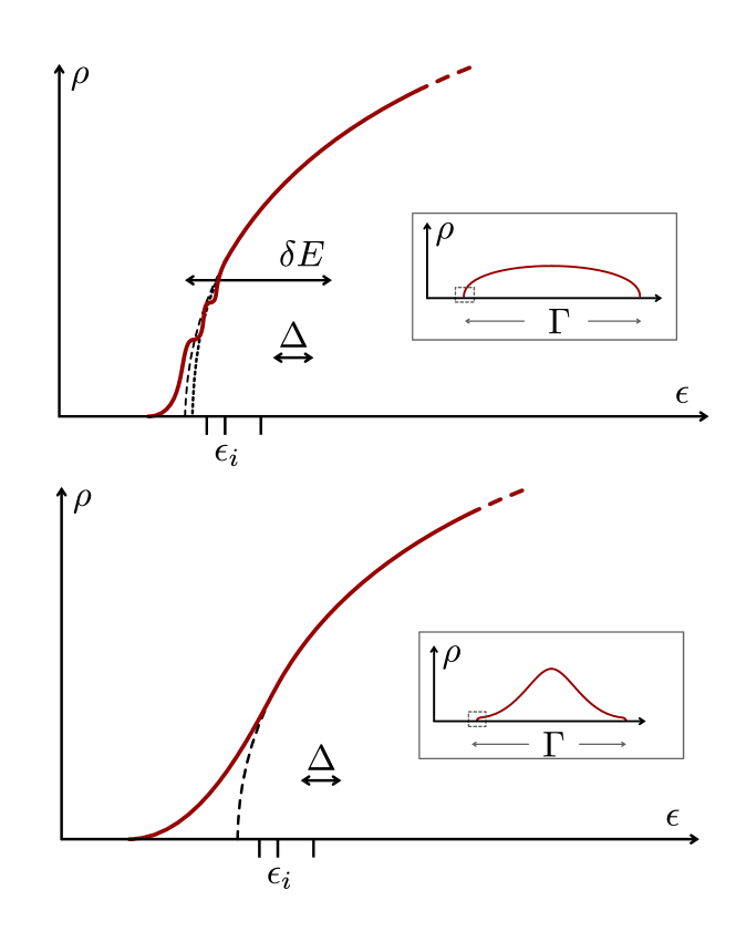
Figure 1: Upper panel: near edge spectral density of dense systems. A small tail and oscillations periodic in $\sim D^{-1}$ well away from the edge superimposed on the $\sim\epsilon^{1/2}$ (long dashed) mean field profile indicate an almost crystalline ordering of levels close to the edge. Inside the edge, there exists a weak universal power law correction $\sim\epsilon^{-5/2}$ (short dashed), which may serve as a perturbative indicator of the dense universality class in physical models such as JT gravity. Bottom: the near edge spectral density of sparse models is softer, structures at level spacing scales are washed out. The spectral density at large scales (inset), too, is broader distributed than it is in the dense case. Here, $\Gamma$ and $\Delta$ are the band width and mean level spacing, respectively, and $\delta E$ is the energy range over which the scaling form of the density of states holds (see also discussion in main text).

In section IV, we will discuss how the differences to the dense case originate in the presence of two channels of correlations in sparse systems. The first of these, can be traced back to statistical dependence: turning only few ‘knobs’ in the Hamiltonian affects an exponentially large number of matrix elements, and in this way generates large scale ‘collective’ fluctuations in the spectrum. The second describes the microscale correlations of nearby levels, as in dense systems. Empirically, we know that these two types of fluctuations operate largely independently of each other. In models affording a high degree of analytical solvability, collective [11, 12] and microscale [13] fluctuations can be treated by tailored methods assuming the form of, e.g., summations over different perturbative diagram classes. Considering the SYK model as a case study, we will here introduce a comprehensive framework in which the fluctuations of a sparse system are treated in a unified fashion. Zooming in to the edge, we will show how the theory assumes the form of a matrix theory different from the Kontsevich model.

We reason that the emergence of two different effective theories reflects the existence of at least two universality classes for the edge transition, dense and sparse. The differences between these two classes become of importance in cases where physical phenomena close to quantum ground states are addressed. As a case study, we will consider the two-dimensional holographic correspondence, which motivated the introduction of the SYK model in the first place [6]. In this context, JT gravity and the SYK model feature representatives of the dense and sparse class, respectively. (The intuition behind the gravity setting in the dense class is that the gravitational path integral describes fluctuating geometries. Thinking of the latter in terms of discrete tessellations of space-time, fluctuating matrix structures containing about as many random parameters as degrees of freedom emerge — a dense scenario.) The finding that the two models fall into different universality classes may be somewhat sobering news for the construction of holographic correspondences relying on principles of chaos: In the regimes of interest, so-called double scaled energy windows close to the band edge, the differences in the structure of bulk (JT) and boundary (SYK) spectra show in the average spectral density as well as in its statistical correlations. Specifically, we will demonstrate that the collective fluctuations affect the spectral form factor (Eq. (28)), including at time scales $\tau\gtrsim 1$, where correlations in the spectrum at level spacing scales are probed. (The statistical independence of collective and micro-scale fluctuations is not in conflict with the former influencing the latter down to the smallest scales.) A fully developed holographic correspondence would not tolerate such differences, and hence require the model sitting in the dense class at the boundary. However, this criterion is not realizable in terms of ‘natural’ theories defined in terms of a few-body interaction. Instead, one needs to resort to more artificial constructions such as the so-called double scaled SYK model [14], where $q$-body interactions with $q$ scaling as a power of $N$, define a dense setting. In section V, we will demonstrate how the structure of the edge interpolates between the sparse and the dense profiles as we increase the large-$N$ scaling of $q$ in an SYK Hamiltonian.

The remainder of the paper is organized as follows: We start in section II with a more precise definition of the spectral edge, and quick introduction of statistical diagnostics that will be used throughout. In sections III and IV we will discuss the near edge physics of dense and sparse systems, respectively. We will compare our predictions to exact diagonalization in section V, and in section VI discuss two-dimensional holography as an application. Several more technical discussions, such as the first principle derivation of the effective edge theories for random matrix Hamiltonian (dense) or the SYK Hamiltonian (sparse) are relegated to Appendices.

II Setting the scene

We start our discussion with a sharpened definition of the terminology ‘spectral edge’. Consider an ensemble of chaotic quantum systems defined in a $D$-dimensional Hilbert space whose spectral density vanishes on average as $\langle\rho(\epsilon)\rangle\approx\bar{\rho}\sim\epsilon^{\alpha}\,\Theta(\epsilon)$, with $0<\alpha<1$. Here, the ‘mean field’ approximation $\bar{\rho}$ is defined to exclude contributions to $\langle\rho\rangle$ vanishing in the limit $D\to\infty$. (Throughout this paper, spectral densities averaged in different ways will appear frequently. Unless stated otherwise, we use the notation $\bar{\rho}$ for the leading order contribution to the spectral density and $\langle\rho\rangle$ for the exact ensemble average. Occasionally, we will need to indicate the type of averaging, such as $\langle\dots\rangle_{\textrm{coll}}$ for the average over ‘collective fluctuations in sparse systems’. If no confusion is possible, we omit the energy argument, $\bar{\rho}(\epsilon)=\bar{\rho}$, etc.) We implicitly define the region of energies over which the above scaling form holds as $\delta E\ll\Gamma$, where $\Gamma$ is the band width of the system. Deep inside the spectrum, individual energy levels are separated by a spacing $\Delta=\langle\rho\rangle^{-1}\sim\Gamma/D$. Upon approaching the edge, the level spacing increases as $\Delta(\epsilon)\sim\Delta_{0}(\Delta_{0}/\epsilon)^{\alpha}$, where $\Delta_{0}$ is the ‘largest’ average level spacing in the system, i.e. the spacing between the two outermost levels, and implicitly defined by the condition $\int_{0}^{\Delta_{0}}d\epsilon\Delta(\epsilon)^{-1}=1$.

The systems considered here are chaotic down to the edge in the sense that for all energies satisfying the condition $\epsilon\gg\Delta(\epsilon)$ spectral correlations are governed by the universal correlation functions of random matrix theory. For Hamiltonians not possessing antilinear symmetries besides hermiticity – the symmetry class considered in this paper –, this implies that the connected two-point correlation function

$$C(\epsilon_{1},\epsilon_{2})\equiv\Delta^{2}(\epsilon)\left\langle\rho\left(\epsilon_{1}\right)\rho\left(\epsilon_{2}\right)\right\rangle_{\textrm{c}},$$ (2)

is given by [3]

$$C(\epsilon_{1},\epsilon_{2})=-\left\langle\left(\frac{\sin s}{s}\right)^{2}\right\rangle_{\textrm{coll}},\qquad s\equiv\pi\omega\langle\rho(\epsilon)\rangle,$$ (3)

where $\epsilon=(\epsilon_{1}+\epsilon_{2})/2$ and $\omega=\epsilon_{1}-\epsilon_{2}$. The physical meaning of the oscillatory correlation function is level rigidity, i.e. an almost uniform spacing of levels with period $\Delta(\epsilon)$. For later reference, we note that this result can be equivalently represented as

$$C(\epsilon_{1},\epsilon_{2})=-K^{2}_{\textrm{sin}}\left(\rho\epsilon_{1},\rho\epsilon_{2}\right)$$ (4)

where $\rho=\langle\rho(\epsilon)\rangle$ and

$$K_{\textrm{sin}}(x,y)=\frac{\sin(\pi(x-y))}{\pi(x-y)},$$ (5)

is the so-called sine-kernel. However, upon relaxing the condition $\epsilon\gg\Delta(\epsilon)$ down to the near edge regime $\epsilon\gtrsim\Delta(\epsilon)$, these results must be adjusted somewhat:

• Eq. (3) requires a sufficiently large ensemble of levels, such that $\langle\rho(\epsilon)\rangle$ remains approximately constant over the correlation interval $\omega$ centered around $\epsilon$. This condition is satisfied far from the edge, $\epsilon\gg\Delta(\epsilon)$. (In a strict sense, Eq. (3) holds in the limit $D\to\infty$, $\Delta\to 0$ at $\omega/\Delta$ fixed. In sections III and IV we will discuss how this result changes upon approaching the edge of dense or sparse systems.

• The notation $\langle\dots\rangle_{\textrm{coll}}$ in Eq. (3) indicates that the background spectral density $\rho(\epsilon)$ featuring in the definition of the dimensionless scaling parameter $s$ may be subject to collective fluctuations [15, 16]. In section IV, we will discuss how for sparse systems the combined inclusion of microscale correlations and collective fluctuations determines the statistics of spectra down to the smallest energy scales.

Having defined the general setting, we now turn to the specific discussion of the two principal universality classes. In both classes, the edge has the status of a quantum critical point, with $\langle\rho(\epsilon)\rangle$ as a symmetry breaking order parameter, and Eq. (2) as an order parameter correlation function. Much as in other critical theories, the scaling regime unfolding near the critical point will be a powerful source of universality. The difference between the two classes has to do with stronger conditions on effective unitary invariance constraining the dense class, as we will discuss in the following.

III Dense systems

We implicitly define the dense universality class through phenomenological equivalence to a Gaussian distributed random matrix Hamiltonian $H$ . (The condition of Gaussianity can be generalized to other unitarily invariant distributions, i.e., distributions depending on functions of $\mathrm{tr}(H^{n})$, without significant changes to the phenomenology discussed below.) Intuitively, one expects these ‘maximally random’ ensembles to model systems whose microscopic Hamiltonian contains a sufficiently large number of independent matrix elements, hence the attribute ‘dense’. (At this point, we remain vague about the threshold required for a crossover into the dense encoding limit. However, in section V we will investigate this question for a class of generalized SYK models with $q$-body interaction, $q\gg 1$.)

In practical terms, the random matrix paradigm implies an ergodicity condition: all observables are required to be invariant under unitary transformations in Hilbert space. In the following, we discuss how this criterion, combined with the interpretation of the edge as a critical point, essentially fixes the near edge theory of the dense class. To illustrate this point, the discussion in this section will be phenomenological, relying only on the above two criteria. (For a complementary microscopic derivation of the same effective edge theory we refer to Appendix A.)

Starting from Eq. (1) as a definition of our order parameter, and representing the trace $\mathrm{tr}(G)=\sum_{\mu}G_{\mu\mu}$ as a sum over the states of an arbitrary Hilbert space basis $|\mu\rangle$, $\mu=1,\dots,D$, it is evident that we need control over correlation functions of the structure $\langle G_{\mu\mu}(\epsilon^{+})\rangle$ and $\langle G_{\mu\mu}(\epsilon_{1}^{\pm})G_{\nu\nu}(\epsilon_{2}^{\pm})\rangle$ where pairwise summation over $\mu,\nu$ is implicit.

To describe the symmetry breaking phenomenon in this setting, we bundle the required data in a four-block diagonal operator $\hat{G}=(\hat{\epsilon}-H\otimes\mathds{1}_{4})^{-1}$, with

$$\hat{\epsilon}=\textrm{diag}(\epsilon_{1}^{+},\epsilon_{2}^{-},\epsilon_{3}^{+},\epsilon_{4}^{-}),$$ (6)

where $\epsilon^{\pm}=\epsilon\pm i\delta$. In the limit $\epsilon_{1}=\dots=\epsilon_{4}\equiv\epsilon$, and for almost all $\epsilon$ (except for those sitting at the poles of $H$), this operator is invariant under similarity transformations, $\hat{G}=T\hat{G}T^{-1}$, $T\in\mathrm{GL}(4)$, up to the infinitesimal symmetry breaking $\delta$. Upon averaging over realizations, we expect a broadening, $\epsilon^{\pm}\to\epsilon\pm i\gamma$ for energies inside the spectral edge, and hence a collapse of the symmetry to $T\to T^{+}\oplus T^{-}$, where $T^{\pm}\in\mathrm{GL}(2)$. Outside the edge, the symmetry remains unbroken. Our goal now is to formulate a minimal theory for this particular type of symmetry breaking phenomenon. We will here proceed in a bootstrap manner by postulating this theory on the basis of symmetry and consistency arguments, to then discuss how it predicts spectral properties in agreement with those of microscopically defined models.

Assume that our correlation functions can be obtained from a partition sum

$$\mathcal{Z}(\hat{\epsilon})\equiv\int dA\,\exp(-S[A,\hat{\epsilon}])$$ (7)

by differentiation in the arguments $\hat{\epsilon}$. In view of the above symmetry, it is natural to expect that the integration degrees of freedom, $A$, are matrices $A=\{A^{\alpha\beta}\}$, $\alpha,\beta=1,\dots,4$ inheriting $\hat{G}$’s transformation under the symmetry as $A\to TAT^{-1}$. There now comes a little twist, namely, we would like the partition sum to be normalized such that for $\epsilon_{1}^{+}=\epsilon_{3}^{+}$ and $\epsilon_{2}^{-}=\epsilon_{4}^{-}$ we have $\mathcal{Z}(\hat{\epsilon})=1$. This normalization (which is often realized via the introduction of replica indices) can be conveniently implemented by ‘grading’ the matrices $A$ [2]: organizing the index $\alpha=(a,s)$ into a causal index $s=\pm=\pm 1$ and a complementary index $a=1,2$, we organize the $a$-blocks of the matrix $A$ such that

$$A=\{A^{ab}\}=\left(\begin{matrix}A^{\mathrm{bb}}&A^{\mathrm{bf}}\cr A^{\mathrm{fb}}&A^{\mathrm{ff}}\end{matrix}\right),$$ (8)

where $A^{\mathrm{bb,ff}}$ are $2\times 2$ complex matrices and $A^{\mathrm{bf,fb}}$ $2\times 2$ matrices of Grassmann variables. The ‘supersymmetry’ thus defined guarantees that in the above limit the functional integral is properly normalized [2]. In this representation, the above symmetry is realized through matrices $T\in\mathrm{GL}(2|2)$, i.e. invertible $4\times 4$ block matrices of the block structure (8). (In our following discussion, normalization by supersymmetry will play only a minor role. What matters conceptually is that our theory has $4\times 4$ matrices as effective integration variables.) The matrix structure of $A$ and $G$ suggests a proportionality $\langle A^{\alpha\alpha}\rangle_{A}\propto\langle G_{\mu\mu}(\epsilon^{\alpha})\rangle_{H}$ where $\epsilon^{\alpha}$ refers to any of the four energy arguments in Eq. (6) and the averaging on the left/right side of the equation is over the $A$-functional/microscopic realizations of $H$.

In the following, the matrix variables $A$ will play the role of an effective order parameter field, conceptually similar to, say, the variable $\phi$ in the $\phi^{4}$-theory approach to magnetism. Furthering this analogy, we now postulate a minimal action controlling the fluctuation behavior of these matrices. First, it is natural to postulate linearity of the action $S$ in the symmetry breaking arguments $\hat{\epsilon}$ (which plays a role akin to a magnetic field in the $\phi^{4}$-analogy). Noting that $A\sim\hat{G}$ carries the effective dimension [energy]^-1, the simplest operator satisfying these conditions reads $S_{\hat{\epsilon}}\equiv c\,\mathrm{str}(A\hat{\epsilon})$ where $c$ is an as yet unspecified constant, and ‘str’ the trace operation for graded matrices[2], $\textrm{str}(A)\equiv\sum_{a}\mathrm{tr}(A^{aa})(-)^{a+1}$. As we are interested in small values of $\epsilon$ near the edge, we do not include terms of $\mathcal{O}(\epsilon^{2})$ in the action. We next ask which operator might produce symmetry breaking $(\langle A\rangle=0)\to(\langle A\rangle\not=0)$ as $\epsilon$ changes sign. The simplest candidate is $c_{3}\,\mathrm{str}(A^{3})$, giving the $A$-action the form of a cubic parabola. With this addition the action will have a local minimum or not, depending on the sign of $\epsilon$, and in this way signal a phase transition. An optional term of second order $c_{2}\,\mathrm{str}(A^{2})$ can be removed by a shift of integration variables, $A\to A+\mathrm{const.}$, and higher order terms will be less relevant in the limit of small $\epsilon$.

We are thus led to consider the action

$$S[A,\hat{\epsilon}]=c\,\left(\mathrm{str}(A\hat{\epsilon})+\frac{1}{3}\mathrm{str}(A^{3})\right),$$ (9)

where we used the freedom of rescaling $A\to\lambda A$ to remove one coupling constant $c_{3}\to c/3$. The action $S[A]$ defines a supersymmetric version of the so-called Kontsevich matrix model [10].

The Kontsevich model provides a universal framework for the description of spectral correlations near the edges of invariant random matrix Hamiltonians or, equivalently, random Hamiltonians with dense encoding. Its microscopic construction detailed in Appendix A implies that from it traces of resolvents are obtained as

$$\langle\mathrm{tr}\,G(\epsilon^{\alpha})\rangle =-\partial_{\epsilon^{\alpha}}Z(\hat{\epsilon}),$$ (10)

$$\langle\mathrm{tr}\,G(\epsilon^{\alpha})\,\mathrm{tr}\,G(\epsilon^{\beta})\rangle =\partial_{\epsilon^{\alpha}\epsilon^{\beta}}Z(\hat{\epsilon}),$$ (11)

where the derivatives are to be evaluated at the unit-normalized configuration $\epsilon^{+}_{1}=\epsilon^{+}_{3},\epsilon^{-}_{2}=\epsilon^{-}_{4}$. (For simplicity, we will mostly consider this configuration, and write $\hat{\epsilon}=\epsilon+\frac{\omega}{2}\tau_{3}$ throughout. The infinitesimal symmetry breaking required for the differentiations Eq.(10) is left implicit in this notation.) In the next two subsections we review how the spectral density and its correlations are obtained from Eqs. (10), followed by integration over the effective $A$-degrees of freedom.

III.1 Spectral density

Referring to Ref. [17] and Appendix D for details, the integration over the $A$-matrices yields the average spectral density as

$$\langle\rho(\epsilon)\rangle=c^{\frac{2}{3}}\left(\tilde{\epsilon}\textrm{Ai}^{2}(-\tilde{\epsilon})+(\textrm{Ai}^{\prime}(-\tilde{\epsilon}))^{2}\right),\qquad\tilde{\epsilon}\equiv\epsilon c^{\frac{2}{3}},$$ (12)

in agreement with the classical result of Ref. [8]. Here, we introduced the dimensionless variable $\tilde{\epsilon}$ with scaling factor $c^{\frac{2}{3}}\sim\Delta_{0}$. This is the function schematically shown in Fig. 1, and in quantitative detail in Fig. 2. Notice how its profile reflects spectral rigidity: the position of the edge is fixed with (almost) level spacing precision at $\epsilon=0$, slight deviations showing in an exponentially small tail leaking beyond the edge. Inside the edge, oscillatory modulations indicate a tendency of the levels to order at a separation scale set by the average level spacing.

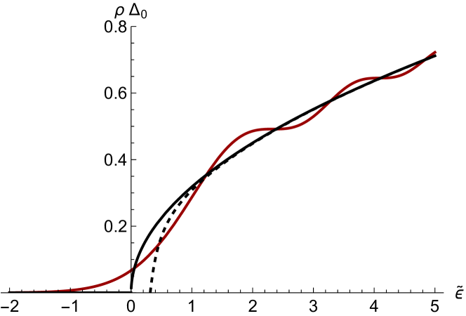
Figure 2: Average spectral density of a dense system near the edge, Eq. (12), expressed as a function of the scaling variable $\tilde{\epsilon}$. The dashed curve includes the correction Eq. (13).

An expansion of the Airy functions in large (negative) arguments then leads to the asymptotic result $\langle\rho(\epsilon)\rangle\approx\frac{c}{\pi}\epsilon^{\frac{1}{2}}$. Up to inessential numerical constants, this leads to the identification $\Delta_{0}\sim c^{-\frac{2}{3}}$ of the near edge level spacing.

However, for our purposes, it will be important to go beyond this approximation and keep track of the first order corrections beyond it. A somewhat tedious computation based on the inspection of the asymptotic expansion leads to the result

$$\langle\rho(\epsilon)\rangle\approx\frac{c^{2/3}}{\pi}\left(\tilde{\epsilon}^{1/2}+\frac{1}{32}\tilde{\epsilon}^{-5/2}+\textrm{osc.}\right),$$ (13)

where ‘osc’ stands for terms oscillatory as $\exp(\frac{i4}{3}\epsilon^{\frac{3}{2}}c)$. In section VI, we will discuss how this result can be understood in perturbation theory by diagrammatic methods, or by topological expansion of the gravitational path integral.

III.2 Stationary phase analysis and spectral correlations

The integration over the full $A$-space may be extended to an exact computation of the second moments Eq. (10), cf. Appendix A. As a result, one obtains

$$C(\epsilon_{1},\epsilon_{2})=-K^{2}_{\textrm{Ai}}(-\tilde{\epsilon}_{1},-\tilde{\epsilon}_{2})$$ (14)

for the connected correlation function (see Fig. 3), where

$$K_{\rm Ai}(x,y)\equiv\frac{{\rm Ai}(x){\rm Ai}^{\prime}(y)-{\rm Ai}(y){\rm Ai}^{\prime}(x)}{x-y}$$ (15)

is the Airy-kernel. For the purposes of our discussion, we will not need this result in full generality. Instead, we focus on analyzing spectral correlations in a scaling limit where the center value $\epsilon$ of the energies $\epsilon_{1,2}^{\pm}$ is kept fixed while the matrix dimension $D$ is scaled to infinity. We are thus probing spectral correlations of a sub-ensemble of levels that can get arbitrarily close to the macroscopic edge but still contains a large number of levels to obtain universal statistics. In this limit, the exact correlation function Eq. (14) reduces to the sinusoidal result Eq. (3) (cf. Fig. 3) with an average density of states depending on the center coordinate.

To see in more explicit terms how this comes about, note that in the above scaling limit, the largeness of $\epsilon\sim D$ invites a stationary phase approach to the matrix integral. The variation of the action $\delta_{A}S[\bar{A}]=0$ leads to the equation

$$\hat{\epsilon}+\bar{A}^{2}=0,$$ (16)

with the solution

$$\bar{A}=\left\{\begin{array}[]{l l}(-\hat{\epsilon})^{1/2}\,,&\epsilon<0,\cr-i\hat{\epsilon}^{1/2}\tau_{3}\,,&\epsilon>0,\end{array}\right.$$

where in the second line we choose branch of the square root that will lead to convergent fluctuation integrals. This solution makes the interpretation of $\epsilon=0$ as the point of a symmetry breaking phase transition with $\bar{A}$ as an order parameter manifest. Above the transition point, the rotational symmetry of the action in the causal $\pm$ space present in the limit of equal energy arguments, $\omega=0$, is broken, as indicated by the appearance of the matrix $\tau_{3}$.

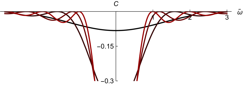
Figure 3: The correlation function Eq. (14) plotted as a function of the difference coordinate $\tilde{\omega}=\tilde{\epsilon}_{1}-\tilde{\epsilon}_{2}$ for the center values $\tilde{\epsilon}=1,4,7,10$ (color coded). Far from the edge (red) the correlation function approaches the sinusoidal behavior of Eq. (3), close to it (black) it diminishes and loses its oscillatory signatures.

Considering energies inside the symmetry broken phase, a shift $A\to\bar{A}+A$ defines the effective fluctuation action $S[A+\bar{A}]=S[\bar{A}]+S_{\textrm{fl}}[A]$, with

$$S_{\textrm{fl}}[A]=c\left(-i\,\mathrm{str}\left(\hat{\epsilon}^{\frac{1}{2}}\tau_{3}A^{2}\right)+\frac{1}{3}\mathrm{str}(A^{3})\right).$$

The largeness of $\epsilon$ implies that generic fluctuations $A$ are gapped by a factor $c\sim D\sqrt{\epsilon}\sim\rho(\epsilon)$. This action may now be applied in different ways to describe the near-edge spectrum.

Perturbation theory:

A straightforward option is perturbation theory in the parameter $\tilde{\epsilon}=\epsilon c^{2/3}$. We here expand in the cubic nonlinearity, followed by Gaussian integration over $A$ applying Wick’s theorem. The advantage of this seemingly redundant approach — we do know the exact answers, after all — is that it provides ‘semiclassical’ clues as to the structure of universal contributions to the spectral density beyond leading order $\rho(\epsilon)\sim\epsilon^{1/2}$. We will discuss this approach, and its applications in the holographic context in section VI.

Double scaling:

Consider the limit where the characteristic energy differences defined by the representation $\hat{\epsilon}=\epsilon\mathds{1}+\frac{\omega}{2}\tau_{3}$ are small in the sense that $\omega$ is of the order of a fixed multiple of the characteristic level spacing $\sim\rho^{-1}(\epsilon)$, and hence of $\mathcal{O}(D^{0})$. In this so-called double scaling limit, generic fluctuations remain gapped in $\sim D$, while the Goldstone mode fluctuations of the symmetry breaking transition become light. To see this in explicit terms, note that in the limit of the absence of explicit symmetry breaking, $\omega\to 0$, generalizations $\bar{A}\to T\bar{A}T^{-1}$ with rotation matrices $T\in\textrm{U}(2|2)$ are solutions of Eq. (16). To leading order in $D^{-1}$, we may thus approximate the effective action as $S[A]\approx S[T\bar{A}T^{-1}]\equiv S[Q]$, where $\bar{A}$ is the above solution of Eq. (16) in the limit $\omega\to 0$. Due to the trace invariance, the cubic term now drops out, and so does the contribution to the energy-vertex proportional to the homogeneous parameter $\epsilon$. We are thus left with the soft mode action

$$S[Q]=-i\pi\bar{\rho}\frac{\omega}{2}\,\mathrm{str}(Q\tau_{3}),$$ (17)

where $\bar{\rho}=\bar{\rho}(\epsilon)=c\epsilon^{\frac{1}{2}}\pi^{-1}$ is the mean field spectral density.

Eq. (17) describes the spectral correlations of generic ergodic quantum systems with average spectral density $\rho(\epsilon)$. Referring to Ref. [2] for a detailed discussion, we note that from this action, the spectral correlation function Eq. (3) is obtained by integration over the manifold of $Q$-matrices.

To summarize, in this section we have reviewed how dense systems display a high level of spectral rigidity, i.e. a near crystalline structure of the spectrum at the scale of the level spacing. These systems are universally described by the simple effective theory Eq. (9). In fact, one may consider this theory as a definition of the dense universality class near a spectral edge. This criterion will become essential in the next section where we discuss ergodic quantum systems outside this class, which are described by a different effective theory.

IV Sparse systems

In the following, we contrast the physics of the rigid edge to that of the softer edge of sparse systems, where the SYK model will be our representative role model. The latter describes $N$ Majorana fermions $\{\chi_{i}\}$, $[\chi_{i},\chi_{j}]_{+}=2\delta_{ij}$, subject to the interaction

$$H =\sum_{ijkl}J_{ijkl}\chi_{i}\chi_{j}\chi_{k}\chi_{l}\equiv\sum_{\sigma}J_{\sigma}X_{\sigma},$$ (18)

$$\sigma=(i,j,k,l),\qquad X_{\sigma}=\chi_{i}\chi_{j}\chi_{k}\chi_{l},$$

where the sum runs over $K\equiv\binom{N}{4}$ four-Majorana index configurations $\sigma$, and the interaction coefficients are Gaussian distributed with variance

$$\left\langle J_{\sigma}J_{\sigma^{\prime}}\right\rangle=\frac{6J^{2}}{N^{3}}\delta_{\sigma\sigma^{\prime}}.$$ (19)

The model is sparse in the sense that it contains only $\mathcal{O}(N^{4})$ statistically independent random coefficients $J_{\sigma}$ in a Hilbert space of dimension $D\equiv 2^{\frac{N}{2}}$, i.e. the Hilbert space of $N/2$ complex fermions of conserved fermion parity. Note how $H$ is an ‘almost diagonal’ operator in that it has matrix elements between fermion occupation number states $|n\rangle,|m\rangle$ of Hamming distance $|n-m|\leq 4$ (i.e. it changes the occupation of at most four fermions). A progressively denser situation may be realized by adding to the Hamiltonian higher $q>4$ interaction vertices, likewise with random coefficients. We will discuss the effect of this generalization in section V.

The fine grained structure of the SYK spectral density has been a subject of intensive research [11, 12, 19]. Specifically, we know that its average is approximately given by

$$\langle\rho(E)\rangle\approx c\exp\left(\frac{2\arcsin^{2}(E/\Gamma)}{\ln\eta}\right),$$ (20)

where

$$\Gamma=2\left(\binom{N}{4}\frac{6}{N^{3}}\right)^{\frac{1}{2}}\frac{J}{1-\eta}\simeq JN$$ (21)

defines the band width, $c$ is a normalization factor, and $\eta\approx\exp(-2q^{2}/N)$ is a constant approaching the value unity in the limit of large $N$. In the center of the distribution, $\rho(E)$ is Gaussian. Referring for a more detailed discussion to Appendix B, this difference to the semicircular spectral density of the dense system, reflects that the Hamiltonian (18) contains only polynomially (in $N$) many operators most of which are commutative. As a consequence, individual many-body levels assume the form of sums of approximately independent random numbers, whose statistics is governed by the central limit theorem[20]. (By contrast, the dense system is described by a much larger number of mutually non-commutative operators.)

Close to the (say, lower) edge, $E\approx-\Gamma$, the distribution ceases to be Gaussian, and an near edge expansion of the spectral density leads to the approximation

$$\langle\rho(\epsilon)\rangle\sim\sinh\left(\frac{2\pi\sqrt{2}}{-\ln\eta}\sqrt{\frac{\epsilon}{\Gamma}}\right)\Theta(\epsilon),$$ (22)

where $\epsilon=E+\Gamma$ measures the distance to the edge. For $\epsilon\ll\Gamma$, we recover a square root singularity $\sim\sqrt{\epsilon}$, as for the dense system.

These results describe the spectral density to leading order in a $N^{-1}$ expansion, i.e. in a limit in which $N\to\infty$ at a fixed ratio $\epsilon/\Gamma$. However, beyond this approximation the interplay of two sources of fluctuations leads to additional deviations from the spectral density of dense systems. We refer to these two as collective, and micro scale fluctuations, respectively.

IV.1 Collective spectral fluctuations

Choosing a different realization of the SYK Hamiltonian changes a polynomial number, $K$, of random parameters in a Hilbert space of exponentially large dimension, $D$. This turning of relatively few ‘knobs’ leads to large sample–to–sample fluctuations of the average spectral density via a mechanism absent in the dense system [16, 21, 22]. The same perturbative construction which underlies Eq. (20) shows that (cf. Appendix B)

$$\mathrm{var}(\rho(\epsilon))=\frac{\langle\rho(\epsilon)\rangle^{2}}{2K}.$$ (23)

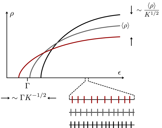
Figure 4: Collective fluctuations cause a blurring of the spectral edge, fluctuations around the average spectral density, and of the average level spacing.

The conservation of the total number of levels suggests an interpretation of these fluctuations in terms of a ‘breathing mode’, i.e. a realization specific scaling of the spectrum as $\epsilon_{\lambda}\to\epsilon_{\lambda}(1+\xi)$ [21], and of the average level spacing, $\Delta\to\Delta(1+\xi)$, see Fig. 4. Assuming a statistical distribution of the parameter $\xi$, comparison with Eq. (23) shows that $\mathrm{var}(\xi)=\frac{1}{2K}$, i.e. a scaling of the spectrum proportional to that of the spectral density. In particular, one expects that the spectral edge, too, is statistically distributed (also cf. Ref. [19]),

$$-\Gamma\to-\Gamma+\delta\epsilon_{0},\qquad\langle\delta\epsilon_{0}\rangle=0,\qquad\textrm{var}(\delta\epsilon_{0})=\frac{\Gamma^{2}}{2K}.$$ (24)

This result implies a softening of the near-edge spectral density as

$$\langle\rho(\epsilon)\rangle\approx\left\langle\sinh\left(2\pi\sqrt{2}\sqrt{\frac{\epsilon-\delta\epsilon_{0}}{\Gamma}}\right)\Theta(\epsilon-\delta\epsilon_{0})\right\rangle_{\delta\epsilon_{0}},$$ (25)

over the Gaussian distribution specified by Eq. (24). In section V we show that this prediction is in excellent agreement with exact diagonalization. In particular, we expect the integration over the breathing mode to eradicate oscillatory signatures in the spectral density.

More generally, table 1 lists the coarse grained differences in the spectral densities of dense and sparse systems, respectively, as caused by this channel of fluctuations. However, before discussing the structure of the spectrum on the highest resolution scales, we need to discuss the complementary microscale correlation channel in the next section.

signature	dense	sparse
collective fluctuations	none	$\mathrm{rms}(\rho)\sim\rho/\sqrt{K}$
tail beyond edge	$\mathcal{O}(D^{-1})$	$\mathcal{O}(\ln(D)^{-2})$
singular power law corrections	yes	no
near edge oscillatory modulation	yes	no

Table 1: Signatures of the average spectral densities for dense and sparse systems, respectively.

Microscale correlations

For a given realization, we expect the spectrum of a sparse system to show strong level repulsion as in the dense case, see Fig. 4 for a qualitative illustration. As we are going to discuss next, this microscale level structure is described by the Goldstone modes of the causal symmetry breaking transition, i.e. the $Q$-modes of our previous discussion, now operating in the sparse context.

Referring to Appendix C for a microscopic construction, the combined effect of microscale and collective fluctuations affords a simple representation in terms of the effective action

$$S[Q]=\ln\left\langle\exp\left(-i\pi\rho(\epsilon)\frac{\omega}{2}\,\mathrm{str}(Q\tau_{3})\right)\right\rangle_{\textrm{coll}},$$ (26)

where the averaging is over the statistically distributed spectral density $\rho(\epsilon)$ with variance (23). This action describes spectral correlations between levels $\epsilon\pm\omega$, where we assume $\epsilon\gg\Delta$. (In view of the large fluctuations, Eq. (24), there exists no edge that could be approached with a precision set by $\Delta$.)

There are different ways to extract information from this representation. One is to integrate over the Gaussian distribution of $\rho$ with variance Eq. (23), to obtain the averaged action

$$S[Q]=-i\pi\langle\rho(\epsilon)\rangle\frac{\omega}{2}\,\mathrm{str}(Q\tau_{3})+\frac{(\pi\omega\langle\rho(\epsilon)\rangle)^{2}}{16K}\,(\mathrm{str}(Q\tau_{3}))^{2}.$$ (27)

One may then obtain the spectral correlation functions by integration over the $Q$-matrices. Due to the high symmetry of the induced quadratic weight, this procedure is not more difficult than the integration over Eq. (17). However, an even more straightforward strategy is to first integrate over $Q$ in Eq. (26), i.e. to compute spectral correlations for a given realization $\rho(\epsilon)$. As a result, one obtains Eq. (3), which in a second step is averaged over $\rho(\epsilon)$.

Either way, the result of these computations, is best discussed in the language of the spectral form factor, i.e. the temporal Fourier transform

$$K(\tau)=\int ds\,e^{is\tau}C(s)$$ (28)

of the spectral correlation function expressed in the energy-like dimensionless variable, $s=\pi\omega\rho$. For Eq. (3), we obtain the familiar result

$$K(\tau)=\tau\Theta(1-\tau)+\Theta(\tau-1),$$

comprising a linear ramp for $\tau<1$ followed by a plateau for larger times.

We may now define the physical form factor through $K_{\mathrm{phys}}(\tau)\equiv\pi\bar{\rho}\langle\tilde{K}(t)\rangle$, where $\tilde{K}(t)\equiv\int d\omega\exp(i\omega t)\langle C_{\rho}(\omega)\rangle$ is the real time Fourier transform of the correlation function (2) and the notation emphasizes that $C_{\rho}(\omega)=C(\epsilon_{1},\epsilon_{2})$ depends on the difference $\omega=\epsilon_{1}-\epsilon_{2}$, and on the center energy through $\rho=\rho(\epsilon)$. In this way, we obtain

$$K_{\mathrm{phys}}(\tau)=\left\langle\frac{\langle\rho\rangle}{\rho}K\left(\tau\frac{\langle\rho\rangle}{\rho}\right)\right\rangle.$$ (29)

The distribution (23) implies that $\langle\rho\rangle/\rho$ is a random variable with average unity, and variance $\mathrm{var}(\langle\rho\rangle/\rho)=1/(2K)$. The most visible influence of the average over the distribution is a rounding, over scales $\sim K^{-1/2}$, of the corner singularity of $K(\tau)$ at $\tau=1$, i.e. at physical time scales of the order of the Heisenberg time $\sim\Delta^{-1}$.

The principle here is that collective fluctuations of the spectral density over large scales let the average level spacing, and hence the oscillation period of the spectral correlation functions at the smallest scales fluctuate as well. The effects of this locking mechanism are witnessed, e.g., by the rounding of the spectral form factor.

V Numerical analysis

In this section we compare the results discussed above to exact diagonalization. We begin with a discussion of the standard SYK model, and then consider a generalized variant where the interaction vertex couples $q>4$ Majorana fermions.

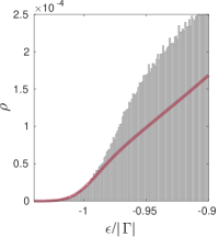
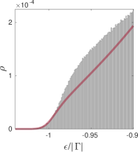
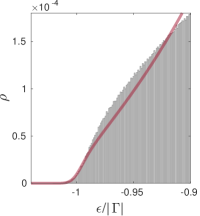
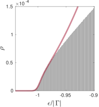
Figure 5: Left to right: Near edge spectral density of the SYK model with $q=4$ and $N=18,\;22,\;26,\;30$. We obtain a progressively better fit to Eq. (25) in terms of two fitting parameters $\Gamma$ and the normalization prefactor (red curves). After removal of fluctuations $\delta\epsilon_{0}$ (see Eq. (24)), the $\sinh$ profile describes the spectral density for $N\geq 30$. The number of realizations here are $50,000$ for $N=18,\;22$ and $10,000$ for $N=26,\;30$, respectively, and fitting parameters for increasing $N$ are $\Gamma=-3.62,\;-4.28,\;-4.96,\;-5.62$.

SYK Model

Fig. 5 shows the near edge spectral density of SYK models with $N=18,\;22,\;26$ and $30$ Majorana fermions. (We increase in steps of $4$ to keep the model in the unitary symmetry class [23].) The red curves are fits to Eq. 25 in terms of two parameters, $\Gamma$ and the overall prefactor omitted in that formula. For increasing $N$, the agreement becomes excellent and extends deeper into the spectrum. We have also checked that for large $N\geq 30$ and after removal of the collective fluctuations of the edge position Eq. (24), the distribution of individual systems follows the $\sinh$-profile of Eq. (25), see also Ref. [12].

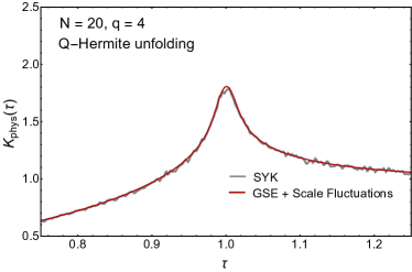
Figure 6: Average connected spectral form factor for $q=4$ SYK spectra (gray curves) for $N=20$ (upper) and $N=28$ which are in the GSE universality class. The results are compared to the analytical GSE result with scale that fluctuates according to a Gaussian with unit average and variance determined by moments of the SYK Hamiltonian. The number of realizations for $N=20$ and $N=28$ is 10,000 and 15,0000, respectively.

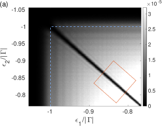
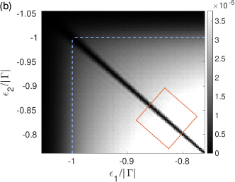
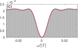
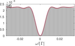
Figure 7: Level-level correlation function $\langle\rho(\epsilon_{1})\rho(\epsilon_{2})\rangle$ for a random matrix ensemble (a) and the SYK model with $q=4$, both acting on Hilbert-spaces of dimension $D=2^{8}$ [24]. Notice the oscillations of the average spectral density in the RMT case. Panels (c) (RMT) and (d) (SYK model) show the corresponding spectral correlations as a function of the relative energy $\omega=\epsilon_{1}-\epsilon_{2}$, averaged along the center energy $\epsilon=(\epsilon_{1}+\epsilon_{2})/2$. In both cases the average over $\epsilon$ leads back to the universal result Eq. (3).

Figure 7 shows the spectral correlations $\langle\rho(\epsilon+\omega/2)\rho(\epsilon-\omega/2)\rangle_{c}$ near the edge, i.e. the correlation function (2) without the normalizing factor $\Delta^{2}(\epsilon)$. Panel (a) shows data in a gray scale representation for an ensemble of random matrices of dimension $D=2^{8}$ and (b) for a SYK model with $N=18$, both averaged over $2\times 10^{5}$ realizations. Upon approaching the edge, the spectral density, and hence its moments, decrease as indicated by the darkening of the color. The main difference between the two correlation profiles is the ripple pattern visible in the RMT case, (a). It is a consequence of the oscillatory modulations of the near edge spectral density, Eq. (15), which extends to the unnormalized correlation function. Another way of stating the same is that the RMT correlation function is given by Eq. (14), which only for energies well inside the spectrum, $\epsilon_{i}\gg\Delta_{0}$ asymptotes to the sine kernel correlation function Eq. (3). Panels (c) and (d) compound the spectral correlations averaged over the center coordinates within the regions indicated by dotted parallelograms in (a) and (b). The data show that both the SYK model and a reference random matrix model retain their sine kernel microscale correlations Eq. (3) in the near edge region.

As discussed in the previous section, collective fluctuations result in a rounding of the spectral form factor at the Heisenberg time. This effect is most pronounced for the Gaussian Symplectic Ensemble (GSE) where the form factor diverges at this point. In Fig. 6, we illustrate this for the connected spectral form factor of the $q=4$ SYK model for $N=20$ (upper) and $N=28$ (lower). The gray solid curves represent the results for the unfolded SYK spectra. They have been unfolded by means of the exact Q-hermite spectral density corrected by an even 8th order Hermite polynomial with coefficients fitted to the ensemble averaged spectral density. This can be justified from the observation that the spectral form factor is local in the sense that only close pairs of eigenvalues result in significant contributions. The exact data are compared to the analytical result (28) with $\mathrm{var}(\langle\rho\rangle/\rho)=1/(2K)$ and $K(x)$ equal to the spectral form factor for the GSE. The agreement is excellent.

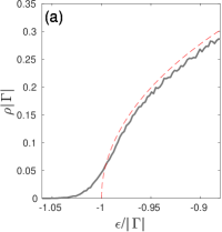
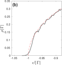
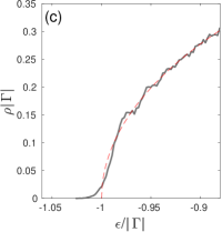
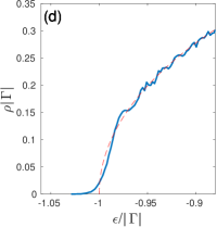
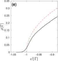
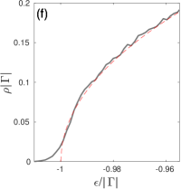
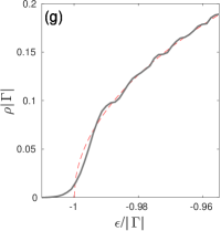
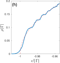
Figure 8: Crossover from sparse to dense spectral statistics probed via the average spectral density of SYK models with $q=4,\;6,\;8$-Majorana interaction for $N=18$ (panels (a-c)) and $N=22$ (panels (e-g)). The guide lines (red dotted) are generated by fitting a semi-circle to the DoS of random matrices of dimensions $D=2^{8}$ and $D=2^{10}$, respectively. The formation of the spectral edge oscillation is clearly seen as $q^{2}/N$ increases for both sizes $N=18,\;22$. Each plot was generated by averaging over an ensemble of 50,000 realizations.

Generalized SYK Model

An increasing of the number of random parameters in a many-body system will eventually induce a crossover between the spectral signatures of sparse and dense systems. To realize this phenomenon, we consider a variant of the SYK Hamiltonian (18)

$$H=\sum_{i_{1}<i_{2}<\cdots<i_{q}}J_{i_{1},\cdots i_{q}}\chi_{i_{1}}\chi_{i_{2}}\cdots\chi_{i_{q}},$$ (30)

containing products of a variable number $q\geq 4$ of Majorana operators. As before, we define the Gaussian variance of the matrix elements through Eq. (19), with $\sigma=(i_{1},\dots,i_{q})$. The spectral density of the generalized model can be calculated [12] by the same methods as in the standard model (cf. Appendix  B), and continues to be given by Eq. (25) with, however, the constant $\eta$ now generalized to

$$\eta=\binom{N}{q}^{-1}\sum_{r=0}^{q}(-1)^{q+r}\binom{q}{r}\binom{N-r}{N-q}\stackrel{{\scriptstyle N\gg q}}{{\approx}}(-1)^{q}e^{-\frac{2q^{2}}{N}}.$$

Figure 8 shows the averaged DoS of SYK models with increasing connectivity $q=4,\;6,\;8$ for $N=18$ (panels (a-c)) and $N=22$ (panels (e-g)). We observe a gradual stiffening of the edge and the onset of oscillations which for $N=18$ and $q=8$ lead to a profile similar to that of a random matrix (panels (d) and (h) for comparison). The onset of the spectrum given by $E_{0}=4\sigma/(1-\eta)$ (with $\sigma$ the width of the spectrum) also approaches the RMT value of $2\sigma$. On general grounds, one expects the crossover from sparse to dense spectral correlations to be driven by the parameter $\lambda\sim q^{2}/N$. (The constant of proportionality is of $\mathcal{O}(1)$ and depends on choice of the variance of the coefficients $J_{\sigma}$.)

VI Application: Two-dimensional holography

While it had been known for a number of years that low-dimensional quantum gravity has a close connection with matrix integrals [25], it has only been appreciated more recently, that the matrix integrals occurring in quantum gravity in fact may have their origin in chaotic dynamics. Early work mainly employed matrix-model machinery as an elegant and efficient tool to define a path integral of discrete triangulations of two-dimensional ‘universes’. However, recently it has become increasingly clear that the random matrices occurring in these constructions in fact have an interpretation as boundary Hamiltonians, in the sense of holographic duality [4].

The prototypical example of such a correspondence between a two-dimensional theory of gravity and random-matrix theory is the so-called JT-theory of gravity, which is perturbatively dual to the ‘SSS matrix’ model [4]. The two-dimensional theory of gravity in question has a semiclassical description starting with the action

$$S_{\rm JT}=-S_{0}\chi({\cal M})-\frac{1}{2}\int_{\cal M}\sqrt{g}\phi\left(R+2\right)-S_{\textrm{bdy}}\,,$$ (31)

where $g$ is the metric, and $R$ the associated scalar curvature. The scalar field $\phi$ is the so-called dilaton, which is present as an extra degree of freedom in JT gravity, and is best understood as a remnant of higher-dimensional gravitational degrees of freedom if viewing JT gravity as a dimensional reduction from higher dimensions [27]. The coefficient $S_{0}$ defines the coupling to the Euler number $\chi\left({\cal M}\right)$ of the manifold ${\cal M}$, the notation emphasizing its identification with an entropy. (Within the framework of the holographic correspondence, $S_{0}$ is the extensive ground-state entropy of the SYK model.) Finally, the boundary action $S_{\rm bdy}\equiv\int_{\partial{\cal M}}du\left({\cal K}-1\right)$ involves the extrinsic curvature ${\cal K}$ of the boundary $\partial{\cal M}$, whose details may be found for example in [4, 28]. It ensures that the action (31) has a well-defined variational principle, as well as a (renormalized) bulk-boundary dictionary.

The duality between (31) and a matrix integral of the form

$$\int dHe^{-V_{\rm SSS}(H)}$$ (32)

has the status of a holographic duality, similar in spirit to the duality between ${\cal N}=4$ supersymmetric Yang-Mills theory and type II string theory on AdS${}_{5}\times$S⁵ [29] with one major departure: while the original examples propose a duality between a fixed individual field theory, namely ${\cal N}=4$ SYM, and a fixed individual bulk theory, namely type IIB superstrings, the JT/SSS duality in fact juxtaposes a (seemingly) fixed individual bulk theory (JT gravity) with an ensemble of boundary theories, the SSS matrix model with the interpretation that the matrix integral is in fact over boundary Hamiltonians. This has spurred much activity attempting to reconcile these two radically different examples of holographic duality, motivated by the possible implication that gravity might microscopically be described by an average over theories, rather than any specific theory. Without entering into the details, which may be found e.g. in [4, 30, 31, 17, 32, 33, 34], we may simply summarize the situation by posing the question “is gravity dual to an ensemble?”. One way to ease this tension between low- and high-dimensional incarnations of the holographic principle, might be an interpretation of the former as lower-dimensional reductions of higher-dimensional parent theories by integration over hidden degrees of freedom. This view is supported, e.g., by the explicit construction of Ref. [28], representing two-dimensional JT gravity as a reduction from a six-dimensional (Calabi-Yau) theory in a manner resembling an ensemble average.

Another possible way to reconcile these two points of view would be to exhibit a fixed quantum mechanical theory whose chaotic behavior is such that it is described by, say, the SSS matrix model – or indeed any other example of a matrix model with a gravitational dual in (bulk) dimension two or three (see [35, 36, 37] for 3D examples) – together with a suitable coarse-graining procedure for low-energy gravity. For this purpose the dense-encoding properties we have proposed above give a new discriminatory criterion to distinguish potential quantum chaotic theories that could give rise to the required averaged physics.

“Natural” candidates for quantum boundary theories in low-dimensional holographic duality would appear to be many-body models subject to few-body random interactions, such as models in the SYK family. Here the issue is made more pressing by the fact that low-dimensional holography unfolds close to the ground states of the theories in question, i.e. precisely the region where the differences between dense and sparse become most acute.

Before commenting further on this point, let us thus briefly review how JT gravity produces results indicative of such densely encoded random systems. This means that we need to understand how spectral properties are formulated in a gravitational language. The quickest way to see spectral statistics expressed in terms of gravitational quantities is via the calculation of multi-resolvent correlators, which are encoded in certain geometries contributing to the path integral with action (31) above, following the original treatment in [4]. In fact, it is more natural in holographic duality to instead work with the Laplace transform and compute the partition function $Z(\beta)$ and its generalization to the multi-resolvent case. We are therefore interested in computing quantities of the type

$$Z(\beta_{1})\cdots Z(\beta_{n})\Bigr{|}_{\rm JT}\,,$$ (33)

given by spacetimes with $n$ boundary circles of length $\beta_{1}\,\ldots,\beta_{n}$, potentially connected to each other by the bulk geometry. In this way, the density of states is related to the JT path integral over surfaces with one boundary, but arbitrary bulk topology

$$Z(\beta)\Bigr{|}_{\rm JT}=\,\,\,\includegraphics[width=130.08731pt,valign={c}]{FIGURES/TopoFig1}\,$$ (34)

Similarly, we may deduce the two-level correlation function from the path integral over two-boundary geometries in JT gravity

$$Z(\beta_{1})Z(\beta_{2})\Bigr{|}_{\rm JT}=$$

Returning to the spectral density we obtain the leading answer from the disk partition function

$$Z_{\rm Schw}^{\rm disk}(\beta)=\frac{e^{\frac{\pi^{2}}{\beta}}}{\sqrt{16\pi\alpha^{3}\beta^{3}}}\,,$$ (35)

resulting in

$$\rho_{0}(E)=\frac{e^{S_{0}}}{(2\pi)^{2}}\sinh\left(2\pi\sqrt{E}\right)\,,$$ (36)

i.e. an expression equal to that of average spectral density of the SYK model Eq. (22) upon identifying the present dimensionless $E$ as the SYK energy measured in units of the band width. However, a closer look reveals differences rooted in the fact that JT is a dense system, while SYK is sparse. These difference emerge, once we push the expansion of the spectral density to one order higher in powers of $e^{-S_{0}}$, i.e. the torus topology indicated in Eq. (34).

Referring to the original references [38, 4] for details, the expansion of the inverse Laplace transform of $Z(\beta)$ defines a topological expansion of the resolvent $R(z)=\mathrm{tr}(G(z))$ of the dual matrix theory as

$$R(z)=\sum_{g=0}^{\infty}\frac{R_{g,1}(z)}{(e^{S_{0}})^{2g-1}}\,,$$ (37)

where $g$ labels the genera of surface geometries, and the subscript ‘1’ in $R_{g,1}$ indicates that we are considering a single boundary.

It has been shown [38, 4, 39] that the first terms of this expansion read

$$R^{\rm JT}(z)=-e^{S_{0}}\frac{\sin(2\pi z)}{4\pi}-e^{-S_{0}}\frac{3+2\pi^{2}z^{2}}{48z^{5}}+{\cal O}\left(e^{-3S_{0}}\right)\,.$$

Taking the imaginary part, we obtain the density of states $\rho(E)=-\frac{1}{\pi}\textrm{Im}R(z)|_{z=\sqrt{E+i0}}$ as

$$\rho^{\rm JT}(E) = e^{S_{0}}\frac{1}{4\pi^{2}}\sinh\left(2\pi\sqrt{E}\right)$$

$$+e^{-S_{0}}\left(\frac{1}{16\pi}E^{-5/2}+\frac{\pi}{24}E^{-3/2}\right)+{\cal O}\left(e^{-2S_{0}}\right).$$

To relate this expression to our earlier discussion of the near edge spectral density predicted by the flavor matrix model, we recall that the asymptotic scaling $\rho(\epsilon)=\frac{c}{\pi}\epsilon^{1/2}$, defined the dimensionless expansion parameter $\tilde{\epsilon}=\epsilon c^{2/3}$, i.e. energy in units of the effective level spacing. Comparison with Eq. (VI) leads to $c=e^{S_{0}}/2$, and hence $\rho^{\textrm{JT}}(\epsilon)=\frac{c^{2/3}}{\pi}(\tilde{\epsilon}^{1/2}+\frac{1}{32}\tilde{\epsilon}^{-5/2})+\dots$, i.e. agreement with the expansion Eq. (13). The ellipses indicate contributions proportional to $e^{-\alpha S_{0}}\tilde{\epsilon}^{\beta}$, subleading in powers of the effective level spacing.

To summarize, both the matrix model and JT gravity contain corrections to the leading order spectral density $\sim\tilde{\epsilon}^{1/2}$ which can be captured by topological expansion. In either case, the next-to-leading order terms, proportional to $\epsilon^{-5/2}$ are described by terms of torus topology, $g=1$. While in the gravitational path integral, these assume the form of a disk with a handle attached, cf. Eq. (34), the corresponding matrix ribbon diagram is shown in Fig. 11. Either way, these diagrams represent the leading order contributions to the expansion of the oscillatory Airy spectral density Eq. (64). However, such contributions are absent in the spectral density of the SYK model, and likely any sparse model for that matter.

The division between dense gravitational bulk systems and sparse quantum boundary theories also shows up in probes of spectral correlations such as the form factor. While the sparse form factor is subject to an average over collective fluctuations, cf. Eq. (29) and Fig. 6, the dense form factor is not.

This section has highlighted physical differences between the behavior of dense random matrix theories and sparsely random quantum chaotic systems, such as the SYK model. These results show that it seems unlikely that there exist sparsely encoded random systems whose chaotic signatures are compatible with those predicted by bulk (pure) gravitational systems, such as JT gravity. Indeed, the perturbative topological expansion of the latter is already known, [4], to be perturbatively equivalent to that of a dense matrix model, and hence different to that of a sparse quantum chaotic system. The analysis here puts this observation on a more general footing: the spectra of sparse systems are subject to collective fluctuations not present in dense systems, and it would thus appear challenging to model pure low-dimensional gravity with a sparse boundary theory.

VII Discussion

In this paper we reasoned that the near-edge physics of chaotic quantum systems generically falls into one of two symmetry classes, sparse or dense. Which of these is realized depends on the ratio between the number of a system’s independent random parameters and the Hilbert space dimension $D$, logarithmic vs. algebraic defining the two cases sparse vs. dense, respectively. What both classes have in common is a non-analytic vanishing of the mean field ($D\to\infty$) spectral density $\bar{\rho}(\epsilon)\sim\epsilon^{\alpha}$, in line with the interpretation of the edge as a symmetry breaking quantum critical point. However, they are described by different near-edge effective ‘Ginzburg-Landau’ theories namely the Kontsevich matrix model (dense), and a nonlinear sigma model modulated by a scalar fluctuation field (sparse), respectively.

Dense systems maintain a quasi-crystalline degree of stiffness throughout the spectrum, implying oscillatory fine structures modulating the mean field spectral density. We discussed a number of different approaches revealing these structures, namely supersymmetric matrix integrals, diagrammatic perturbation theory, and gravitational path integrals.

Conversely, in sparse systems a much smaller averaging parameter space is responsible for large sample-to-sample ‘collective’ fluctuations in the spectral density. Individual system representatives still feature level repulsion in a sequence terminating in an extremal energy level. However, the position of these terminal points is subject to large fluctuations (in $\ln D$ ), generating tails in the average spectral density and eradicating oscillatory fine structures. We considered the SYK model as a representative case study to demonstrate the statistically independent presence of two channels of fluctuations, the above collective fluctuations, and microscale fluctuations reflecting level repulsion. As a precision test we considered the non-perturbative structure of the spectral form factor and demonstrated parameter-free agreement between exact diagonalization and the predictions of the two-fluctuation channel effective theory.

Finally, we reasoned that while typical few-body interacting many-particle systems are sparse, low-dimensional gravity is dense. This observation is troubling inasmuch as it appears to limit the scope of the holographic correspondence between gravitational bulks and quantum boundary theories realized in terms of ‘natural’ many body systems. This disparity must likely be seen in the context of the still somewhat mysterious status of the ensemble average in low-dimensional holography and calls further study.

Acknowledgments A.A. and K.W.K are grateful for numerous discussions with M. Berkooz on the interpretation of chord diagram statistics. T. M. acknowledges financial support by Brazilian agencies CNPq and FAPERJ. K.W.K is supported by the National Research Foundation of Korea (NRF) grant funded by the Korea government(MSIT) (No.2020R1A5A1016518). A.A. and M.R. acknowledge support from the Deutsche Forschungsgemeinschaft (DFG) Project No. 277101999, CRC 183 (project A03). Antonio M. García-García is thanked for eigenvalue data for $N=28$, and J. J. M. V. is supported in part by U.S. DOE Grant No. DE-FAG-88FR40388. Data and materials availability: Raw data, data-analysis, and codes used in the generation of Fig.5,7,8 are available in Zenodo with the identifier 10.5281/zenodo.10827097 [40].

Appendix A Matrix theory details

For the sake of completeness, we here review the construction of the ‘flavor dual’ of a Gaussian distributed ‘color’ random matrix model (for a more detailed discussion, see Ref. [2]). We consider an ensemble of Gaussian distributed random Hamiltonians, $H=\{H_{\mu\nu}\}$, $\mu,\nu=1,\dots,D$ with second moment

$$\left\langle H_{\mu\nu}H_{\nu^{\prime}\mu^{\prime}}\right\rangle\equiv\frac{\lambda^{2}}{D}\delta_{\mu\mu^{\prime}}\delta_{\nu\nu^{\prime}}.$$ (39)

Our starting point is the Gaussian integral

$$Z(\hat{\epsilon})=\int d\psi\,\left\langle\exp(-S[H,\psi,])\right\rangle,$$ (40)

$$\quad S[H,\psi]\equiv i\bar{\psi}(\hat{\epsilon}-H)\psi,$$ (41)

where $\psi=\{\psi_{\mu}^{\alpha}\}$, $\alpha=(a,s)$ are complex commuting ($\psi^{\textrm{b},s}$) or Grassmann valued ( $\psi^{\textrm{f},s}$ ) integration variables. In this way it is guaranteed that for $\epsilon^{\textrm{b},s}=\epsilon^{\textrm{f},s}$ the integral is unit-normalized. The conjugate variable $\bar{\psi}\equiv\psi^{\dagger}\tau_{3}$ contains a Pauli matrix in the space of advanced and retarded indices ($\mathrm{Im}\,\hat{\epsilon}=i\delta\tau_{3}$) safeguarding the convergence of the integral. (For Grassmann variables, convergence is not an issue and $\psi^{\dagger}$ a symbol for a variable independent of $\psi$.)

Integrating over the $H$-ensemble, we obtain a quartic action

$$Z(\hat{\epsilon})=\int d\psi\,\exp\left(i\bar{\psi}\hat{\epsilon}\psi-\frac{\lambda^{2}}{2D}\mathrm{str}(B^{2})\right),$$ (42)

where the bilinear $B\equiv\tau_{3}^{1/2}\psi_{\mu}\bar{\psi}_{\mu}\tau_{3}^{1/2}$. We decouple this term by a Hubbard-Stratonovich transformation, and do the Gaussian integral over $\psi$ to arrive at

$$Z(\hat{\epsilon})=\int dA\,\exp(-S[A]),$$ (43)

$$\quad S[A]\equiv D\left(\frac{1}{2\lambda^{2}}\mathrm{str}A^{2}+\mathrm{str}\ln(\hat{\epsilon}-A)\right),$$ (44)

where $A=\{A^{\alpha\beta}\}$ is a four-dimensional graded matrix.

The global factor $D$ upfront invites a stationary phase analysis. We first seek a solution for identical energy arguments, $\hat{\epsilon}=E+i\delta\tau_{3}$, except for the important imaginary increment $\pm i\delta$. The variational equation $\delta_{A}S[\bar{A}]=0$ then assumes the form

$$\bar{A}=\frac{\lambda^{2}}{\epsilon+i\delta\tau_{3}-\bar{A}}\Rightarrow\bar{A}=\frac{E}{2}-i\tau_{3}\lambda\left(1-\left(\frac{E}{2\lambda}\right)^{2}\right)^{\frac{1}{2}},$$

where the sign of $\delta$ determines the branch of the square root function. For decreasing energy, $E$, the magnitude of the symmetry breaking imaginary part diminishes, and eventually vanishes at the spectral edges $E=-2\lambda$. The edge theory is obtained by expansion of the action in fluctuations $A\to\bar{A}+A$ around the lower edge configuration, $\bar{A}=-E/2=\lambda$ [43]. Re-introducing a matrix of general near-edge energy configurations, $\hat{\epsilon}\to 2\lambda+\hat{\epsilon}$, an expansion to leading order in fluctuations, then leads to $S[A]=-D\mathrm{str}\left(\frac{\hat{\epsilon}A}{\lambda^{2}}+\frac{A^{3}}{3\lambda^{3}}\right)$, and a final rescaling $A\to A\sqrt{\lambda}$ brings the action into the form of Eq. (9) with the coupling constant $c=D/\lambda^{3/2}$.

Appendix B Collective spectral fluctuations from chord diagrams

Referring to Ref. [21] detailed discussion, we here review how the average spectral density of the SYK model, and its collective fluctuations are described in perturbation theory. To start with, consider the configurational average of a single resolvent, formally expanded in the Hamiltonian

$$\langle\mathrm{tr}\,G(z)\rangle=\sum_{l}z^{-2l+1}\langle\mathrm{tr}_{\mathcal{F}}(H^{2l})\rangle.$$ (45)

We now average over the distribution (19) of the coupling coefficients to generate a series, which up to fourth order reads as

$$\langle\mathrm{tr}\,G(z)\rangle=\frac{D}{z}+\frac{1}{z^{3}}\langle\mathrm{tr}_{\mathcal{F}}(H^{2})\rangle+\frac{1}{z^{5}}\langle\mathrm{tr}_{\mathcal{F}}(H^{4})\rangle+\dots$$

$$\quad=\frac{D}{z}+\frac{\gamma^{2}}{z^{3}K}\sum_{\sigma}\mathrm{tr}_{\mathcal{F}}(X_{\sigma}^{2})$$

$$+\frac{\gamma^{4}}{z^{5}K^{2}}\sum_{\sigma\sigma^{\prime}}\mathrm{tr}_{\mathcal{F}}(X_{\sigma}^{2}X_{\sigma^{\prime}}^{2}+X_{\sigma}X_{\sigma^{\prime}}^{2}X_{\sigma}+X_{\sigma}X_{\sigma^{\prime}}X_{\sigma}X_{\sigma^{\prime}})$$

$$\quad=\frac{D}{z}+\frac{D\gamma^{2}}{z^{3}}+\frac{D\gamma^{4}}{z^{5}}\left(2+\frac{1}{K^{2}}\sum_{\sigma,\sigma^{\prime}}s_{\sigma,\sigma^{\prime}}\right),$$ (46)

with the sign factors defined through $X_{\sigma}X_{\sigma^{\prime}}=s_{\sigma,\sigma^{\prime}}X_{\sigma^{\prime}}X_{\sigma}$, and where

$$\gamma=\left(\frac{6KJ^{2}}{N^{3}}\right)^{\frac{1}{2}}\approx\frac{N^{1/2}J}{2}.$$ (47)

These few terms (cf. Fig. 9 for a visualization) already illustrate the principles of the perturbative analysis: at $2^{\rm nd}$ order in the expansion, we have $(2n-1)!!$ contractions, leading to different combinations, $\dots X_{\sigma}X_{\sigma^{\prime}}X_{\sigma^{\prime\prime}}\dots$, with pairwise occurrences of $\dots X_{\sigma}\dots X_{\sigma}\dots\,$. Reordering them to make use of the self-annihilation $X_{\sigma}^{2}=1$, we need to permute operators $X_{\sigma}X_{\sigma^{\prime}}$ (cf. diagram (2c), or the last term in the third line of the above second order expansion) which introduces sign factors $K^{-2}\sum_{\sigma\sigma^{\prime}}s_{\sigma,\sigma^{\prime}}=1-\mathcal{O}(N^{-1})$, where the deviation of $\mathcal{O}(N^{-1})$ is due to the few configurations where $\sigma$ and $\sigma^{\prime}$ have an odd number of Majoranas in common, and hence anti-commute.

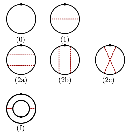
Figure 9: Chord diagrams of zeroth (0), second (1), and quartic order (2a-c) in $H$ contributing to the average spectral density. Diagram (f) describes the leading order contribution to the collective fluctuations, where the solid lines represent the summation of all diagrams contributing to the average spectral density.

Ignoring these corrections, the expansion assumes the form of an asymptotic series, $\langle\mathrm{tr}\,G(z)\rangle\simeq\frac{D}{z}\sum_{n}(\gamma/z)^{2n}(2n-1)!!$. Its combinatorial divergence can be dealt with by Borel resummation [43], i.e. we use the identity $(2n-1)!!=(2\pi)^{-1/2}\int dt\,e^{-t^{2}/2}t^{2n}$, to represent the result as

$$\langle\mathrm{tr}\,G(z)\rangle\approx\frac{D}{\sqrt{2\pi}z}\int dt\,e^{-\frac{t^{2}}{2}}\frac{1}{1-(\gamma t^{2}/z)^{2}}$$

$$\qquad=-\frac{iD\sqrt{\pi}}{\sqrt{2}\gamma}\exp\left(-\frac{z^{2}}{2\gamma^{2}}\right),$$

where we assumed $\mathrm{Im}\,z>0$. With the identification $z=\epsilon^{+}$, we conclude that to leading order in an $N^{-1}$-expansion, the spectral density is Gaussian. The inclusion of corrections due to the above commutators requires more work [12] and leads to the result (20).

Finally, fluctuations of the DoS are described by the diagram (f), where the fat lines represent the summation of all chords contributing to the average $\langle\rho\rangle$. Relative to these, chords connecting between the two propagators come at the expense of missing factors $K\gg 1$, implying that it is sufficient to work to the lowest non-vanishing order, two connecting chords.

Following Ref. [44] the computation of this diagram yields

$${\rm var}(\rho(\epsilon)) \approx\frac{1}{2K}[\partial_{\epsilon}\epsilon\rho(\epsilon)]^{2}.$$ (48)

To see this, consider the formal expansion Eq. (45) and note that non-vanishing diagrams $\langle{\rm tr}(H^{k}){\rm tr}(H^{m})\rangle_{\rm 2cc}$ have both of the connecting chords (2cc) locked to the same four-Majorana index $J_{\sigma}=J_{\sigma^{\prime}}$. Otherwise, the leading order contribution to each individual product $H^{k}$ and $H^{m}$ contains the unpaired Majorana operators $X_{\sigma}$ and $X_{\sigma^{\prime}}$ implying vanishing of their traces. Noting that $H$ contains a summation over $K$ four-Majorana indices, this rationale leads to [21], $\langle{\rm tr}(H^{k}){\rm tr}(H^{m})\rangle_{\rm 2cc}\approx\frac{km}{2K}\langle{\rm tr}(H^{k})\rangle\langle{\rm tr}(H^{m})\rangle$, where the combinatorial factor accounts for the possibilities of choosing two connecting chords within each trace, $\frac{k}{2}\times\frac{m}{2}$, and the two ways of connecting the later. Using this approximation in the expansion Eq. (45), the estimate Eq. (48) follows.

Linearizing on the other hand $\rho_{\xi}(\epsilon)=\frac{1}{1+\xi}\rho\left(\frac{\epsilon}{1+\xi}\right)$ in the spectral shift parameter, $\rho_{\xi}(\epsilon)\approx\rho(\epsilon)-\xi\partial_{\epsilon}\epsilon\rho(\epsilon)$, one finds

$${\rm var}(\rho(\epsilon)) \approx\rm{var}(\xi)[\partial_{\epsilon}\epsilon\rho(\epsilon)]^{2},$$ (49)

indicating that ${\rm var}(\xi)=1/(2K)$. Finally, neglecting contributions from derivatives of the DoS one arrives at Eq. (23) stated in the main text.

Appendix C Effective matrix theory of the SYK model

C.1 Derivation of the matrix action

We here derive the effective matrix action Eq. (26) describing the SYK model after ensemble averaging [13]. Our starting point is again the Gaussian integral representation Eq. (40), only that the Hamiltonian is now the SYK Hamiltonian $H=\{H_{nm}\}$ in a first quantized representation (i.e. interpreted as a matrix acting in a $D$-dimensional Fock space, $\mathcal{F}$, in the fermion occupation number basis $\{|n\rangle\}$) and the averaging is over the Gaussian distributed coupling constants $J_{a}$ in Eq. (18). Doing the averaging, we obtain an action as in Eq. (42), where the $B$-dependent part now assumes the form

$$\frac{3J^{2}}{N^{3}}\sum_{\sigma}\mathrm{STr}(BX_{\sigma}BX_{\sigma}),\qquad B_{mn}=\tau_{3}^{\frac{1}{2}}\psi_{m}\bar{\psi}_{n}\tau_{3}^{\frac{1}{2}}.$$ (50)

Here, $(X_{\sigma})_{mn}$ represent the Majorana quartets $X_{\sigma}$ in Eq. (18) in terms of $D$-dimensional matrices, and the trace $\mathrm{STr}\equiv\,\mathrm{tr}_{\mathcal{F}}\,\mathrm{str}$ extends over both Fock-color and flavor space. We note that the sparsity of the randomness shows in two complications: we generate a sum over a large number of quartic terms indexed by the $\mathcal{O}(N^{4})$ labels $\sigma$, and the building blocks $B$ no longer are ‘color singlets’, but possess matrix structure in both color/Hilbert space ($m$-indices), and flavor space (the $\alpha$-indices implicit in $\psi$).

To mitigate the first of these problems, we use that [13] every matrix $O=\{O_{nm}\}$ in $D=2^{N/2}$-dimensional Fock space (we here consider the entire Fock space of $N/2$ fermions, including both parity sectors) can be expanded in the basis of $D^{2}$ matrices $X_{\mu}\equiv\chi_{\mu_{1}}\chi_{\mu_{2}}\dots$, where the multi-index $\mu$ runs through all of the $2^{N}=D^{2}$ possible combinations labeling distinct Majorana monomials, $1,\chi_{i},\chi_{i}\chi_{j},\dots$. (We reserve the subscript $\sigma$ for matrices $X_{\sigma}$ containing the fixed number of $4$ operators, as in the SYK Hamiltonian.) This expansion reads as [13]

$$O=\frac{1}{D^{\frac{1}{2}}}\sum_{\mu}o_{\mu}X_{\mu},\qquad o_{\mu}=\frac{1}{D^{\frac{1}{2}}}\mathrm{tr}_{\mathcal{F}}(OX_{\mu}^{\dagger}),$$

where we used the orthogonality relation $\mathrm{tr}_{\mathcal{F}}(X_{\mu}X_{\nu}^{\dagger})=\delta_{\mu\nu}D$, and the coefficients $m_{\mu}=\{m_{\mu}^{\alpha\beta}\}$ are matrices in flavor space.

As a direct consequence of this representation change we obtain a decoupling identity similar to a Fierz transform [12],

$$\sum_{\sigma}{\rm tr}_{\cal F}\left(OX_{\sigma}OX_{\sigma}\right)=\frac{1}{D}\sum_{\mu}\sum_{\sigma}{\rm tr}_{\cal F}\left(X_{\mu}X_{\sigma}X_{\mu}X_{\sigma}\right)o_{\mu}^{2}.$$ (51)

Defining two sign factors through $s_{\mu}=X_{\mu}X_{\mu}$ and $X_{\nu}X_{\mu}=s_{\nu,\mu}X_{\mu}X_{\nu}$, we have ${\rm tr}_{\cal F}\left(X_{\mu}X_{\sigma}X_{\mu}X_{\sigma}\right)=Ds_{\sigma,\mu}s_{\mu}$ and with

$$S_{\mu}\equiv\frac{1}{K}\sum_{\sigma}s_{\sigma,\mu},$$ (52)

the trace identity assumes the form

$$\sum_{\sigma}\mathrm{STr}\left(OX_{\sigma}OX_{\sigma}\right)=K\sum_{\mu}s_{\mu}S_{\mu}o_{\mu}^{2}.$$

We now apply this identity to the case where $O\to(3J^{2}N^{-3})^{1/2}B$ contains our bilinears in Eq. (50) with their internal flavor matrix structure. As a result, we obtain

$$\frac{3J^{2}}{N^{3}}\mathrm{STr}(BX_{\sigma}BX_{\sigma})=\frac{3J^{2}K}{N^{3}}\sum_{\mu}s_{\mu}S_{\mu}\mathrm{str}(b_{\mu}^{2})\equiv S[b].$$

This representation is advantageous, in that it contains the essential structure governing the expansion of the theory – the sign factors $S_{\mu}$ describing the degree of non-commutativity of general Majorana monomials $X_{\mu}$ with the quartets appearing in the Hamiltonian via Eq. (52) – as Gaussian weights. However, it still contains the integration variables, in quartic order, via the bilinears $b_{\mu}$.

To remedy this latter problem, we perform a Hubbard-Stratonovich decoupling in terms of $D^{2}$ matrices $a_{\mu}=\{a_{\mu}^{\alpha\beta}\}$. Using that $\mathrm{str}(a_{\mu}b_{\mu})=\bar{\psi}\tau_{3}^{\frac{1}{2}}a_{\mu}\tau_{3}^{\frac{1}{2}}\psi$, it is straightforward to show that

$$e^{-S[b]}=\int Da\,e^{-\frac{1}{2}\sum_{\mu}s_{\mu}S_{\mu}^{-1}\mathrm{str}(a_{\mu}^{2})-i\gamma\bar{\psi}A\psi},$$

where $A=\frac{1}{\sqrt{D}}\sum_{\mu}X_{\mu}a_{\mu}$, $Da=\prod_{\mu}da_{\mu}$, the coefficient $\gamma$ is defined in Eq. (47), and we approximated $K\approx N^{4}/4!$. Finally, the integration over the now quadratic $\psi$-dependence gets us to the effective action

$$S[a] =\frac{1}{2}\sum_{\mu}s_{\mu}S_{\mu}^{-1}\mathrm{str}(a_{\mu}^{2})+\mathrm{STr}\ln\left(\hat{\epsilon}+\gamma A\right),$$ (53)

where the trace of the logarithm extends over both color and flavor space.

So far, all manipulations have been exact. As with the Gaussian distributed matrix model, the action describing the ensemble average over SYK Hamiltonians assumes the form of a quadratic term plus a tr ln. A stationary phase approximation [13] would then lead to a quadratic equation, and the prediction of a semicircular spectral density. While this result is qualitatively correct in the band center, it fails at the band edge. The problem with the stationary phase approach is that in the sparse system, we have a large number of integration degrees of freedom in addition to the single Fock-space homogeneous Goldstone mode $a_{0}$. While these may be individually ‘massive’, they do determine the profile of the spectral density, and in particular describe the collective spectral fluctuations discussed in the main text.

C.2 Collective spectral fluctuations from the matrix action

In the following, we show how to describe the joint effect of microscale correlations (the mode $a_{0}$) and collective fluctuations (all other modes $a_{\mu\not=0}$) in a unified manner starting from Eq. (53). We note that many of the concepts applied here to the SYK model were pioneered in the paper [43].

For this purpose, it will be sufficient to start from a simplified version of the integral in which we work only with the $s=+1$ sector. We consider Eq. (10) at $\alpha=1$, or $\epsilon^{1}=\epsilon_{1}^{+}$ and represent the derivative in $\epsilon_{1}$ at the symmetric point $\epsilon_{1}^{+}=\epsilon_{3}^{+}\equiv\epsilon^{+}$, as $\partial_{\kappa}|_{\kappa=0}$, where $\hat{\epsilon}\to\epsilon^{+}\mathds{1}_{2}+\kappa P$, and $P^{\alpha\beta}=\delta^{\alpha 1}\delta^{\beta 1}$ is a projector onto the first of the four flavor indices. An expansion to the first order in $P$ then is equivalent to taking the derivative.

With this replacement, and $z=\epsilon^{+}$ we consider the expression $G^{+}(z)=\partial_{\kappa}|_{\kappa=0}Z(\kappa)$, where $Z(\kappa)=\left\langle\exp\left(-\mathrm{STr}\ln\left(z+\kappa P+\gamma A\right)\right)\right\rangle$, and

$$\langle\dots\rangle=\int Da\,e^{-\frac{1}{2}\sum_{\mu}s_{\mu}S_{\mu}^{-1}\mathrm{str}(a_{\mu}^{2})}(\dots).$$

We aim to understand how the expansion in $\gamma$ relates to the chord diagram expansion of the spectral density reviewed in section B. With $G_{\kappa}\equiv(z+\kappa P)^{-1}$, we obtain $Z=Z^{(0)}+Z^{(2)}+Z^{(4)}+\dots$, where

$$Z^{(0)}(\kappa) =\exp(-\mathrm{STr}\ln(G_{\kappa})),$$

$$Z^{(2)}(\kappa) =\frac{\gamma^{2}}{2}\left\langle(\mathrm{STr}(G_{\kappa}A))^{2}+\mathrm{STr}((G_{\kappa}A)^{2})\right\rangle,$$

$$Z^{(4)}(\kappa) =\frac{\gamma^{4}}{4}\left\langle\mathrm{STr}((G_{\kappa}A)^{2})(\mathrm{STr}(G_{\kappa}A))^{2}+\mathrm{STr}((G_{\kappa}A)^{4})\right\rangle.$$

(The application of the Wick contraction outlined below to fourth-order combinations such as $(\mathrm{STr}(G_{\kappa}A))^{4}$ or $\mathrm{STr}(G_{\kappa}A)\mathrm{STr}(G_{\kappa}A)^{3}$ leads to products of supertraces $\mathrm{STr}(\dots)\mathrm{STr}(\dots)\dots$, instead of a single $\mathrm{STr}$. After expansion to first order in $P$ we are left with factors $\mathrm{STr}(G_{0})$. The proportionality of $G_{0}$ to unity in graded space implies the vanishing of these terms.) We next need to compute the integrals over the Gaussian weight, and to this end we use a Wick contraction formula for the $2\times 2$-matrices $a_{\mu}$, which can be checked by straightforward computation

$$\langle\mathrm{str}(a_{\mu}Xa_{\nu}Y)\rangle=\delta_{\mu\nu}S_{\mu}s_{\mu}\,\mathrm{str}(X)\mathrm{str}(Y),$$

$$\langle\mathrm{str}(a_{\mu}X)\mathrm{str}(a_{\nu}Y)\rangle=\delta_{\mu\nu}S_{\mu}s_{\mu}\,\mathrm{str}(XY).$$

We also note that the proportionality $G_{\kappa}\propto\mathds{1}_{\mathcal{F}}$ implies $\mathrm{STr}(G_{\kappa}A)=D^{1/2}\mathrm{str}(G_{\kappa}a_{0})$. With these auxiliary identities, we find $Z^{(0)}\to-Dz^{-1}\kappa$, where the arrow stands for the first order expansion in $\kappa$, and we noted $\mathrm{str}(P)=1$. The first order term becomes $Z^{(2)}=\frac{\gamma^{2}}{2}D\,\mathrm{str}(G_{\kappa}^{2})\to-\frac{D\gamma^{2}}{z^{3}}\kappa$, where we used $S_{0}=s_{0}=1$. Finally, the second order term yields

$$Z^{(4)} =\frac{\gamma^{4}}{4}\mathrm{str}(G_{\kappa}^{4})$$

$$\qquad\left(2D+\sum_{\mu\nu}s_{\mu}s_{\nu}S_{\mu}S_{\nu}\frac{1}{D^{2}}\mathrm{tr}_{\mathcal{F}}(X_{\mu}X_{\nu}X_{\mu}X_{\nu})\right)\to$$

$$\qquad\to-\frac{\gamma^{4}\kappa}{z^{5}}\left(2D+\frac{1}{D}\sum_{\mu\nu}s_{\mu}s_{\nu}S_{\mu}S_{\nu}s_{\mu,\nu}\right).$$

Using the definition (52) one can verify that $\sum_{\mu\nu}s_{\mu}s_{\nu}S_{\mu}S_{\nu}s_{\mu,\nu}=\frac{D^{2}}{K^{2}}\sum_{\sigma,\sigma^{\prime}}s_{\sigma,\sigma^{\prime}}$. With these results, we find that the expansion of the resolvent in $a$-mode fluctuations, $\langle G(z)\rangle=\partial_{\kappa}Z(\kappa)$ is identical to that in chord diagrams, Eq. (B). More generally, it is straightforward to verify that the Wick contraction $\langle\mathrm{STr}(XAYA)\rangle$ of $a$-insertions is equivalent to the insertion of an $H$-contraction between the Fock space matrices $X$ and $Y$.

The conclusion here is that individual $a$-contractions represent the chord lines of the original SYK model. At the same time, it is not possible to compute the $a$-integrals to arbitrary order and in closed form. Instead, we here adopt a pragmatic approach. Consider the integration organized in such a way that we integrate over fluctuations diagonal in causal space, $a^{ss}$, first. In a second step, we then consider $a^{s\bar{s}}$, anticipating that generic fluctuations coupling between different causal branches are suppressed in powers of $K$, cf. the reasoning at the end of Appendix B. The exception to this rule are the modes $a^{+-}_{0}$ and $a^{-+}_{0}$, isotropic in Hilbert space, which require a separate treatment. Turning back to the modes $a^{ss}$, it is straightforward, if tedious, to check that the expansion of the tr ln, followed by integration against the Gaussian weight, reproduces the chord diagram expansion. (As it should, so far, no approximations have been made.) This observation has two consequences: first, after resummation, the resolvent Green function (i.e. the formal inverse of the operator under the logarithm) is dressed by a ‘self energy’ whose imaginary part carries a sign factor $(-1)^{s}$. This is the formal statement of symmetry breaking. From a theory with infinitesimal $is\delta$, we proceed to one with finite difference between the retarded and advanced contour. Second, the imaginary part of that Green function yields the cord diagram spectral density, discussed above.

On this basis, we may then proceed to the integration over the modes $a_{0}^{+-}$ and $a_{0}^{-+}$. Being isotropic in color space and off-diagonal in $s$-space they are the Goldstone modes of the above symmetry breaking and must be treated non-perturbatively. To this end, we introduce an off-diagonal $4\times 4$ matrix zero mode generator $W$, defined to anti-commute with the symmetry breaking matrix, $[W,\tau_{3}]_{+}=0$. With $T=\exp(W)$, we change variables, $a_{0}\to T(a_{0}^{++}\oplus a_{0}^{--})T^{-1}$. Likewise, $a_{\mu}\to Ta_{\mu}T^{-1}$, for all Hilbert space inhomogeneous modes, $\mu\not=1$. In this representation, the Goldstone mode generators enter in a form conceptually similar to that of a rotation degree of freedom in a symmetry broken ferromagnetic phase (small energy differences, $\omega$ playing the role of a symmetry breaking magnetic field, in this analogy). Furthering this analogy, we substitute the new representation into (53), and turn to a rotated frame,

$$S[a,T] =\frac{1}{2}\sum_{\mu}s_{\mu}S_{\mu}^{-1}\mathrm{str}(a_{\mu}^{2})+\mathrm{STr}\ln\left(T^{-1}\hat{\epsilon}T+\gamma A\right),$$ (54)

where we noted the $T$-independence of the Gaussian weight, and the matrix $a_{0}$ now excludes the off-diagonal sector. Formally defining the effective Goldstone mode action by an integral over the ‘radial degrees of freedom’,

$$\exp(-S[T])\equiv\langle\exp(-\mathrm{STr}\,\ln\left(T^{-1}\hat{\epsilon}T+\gamma A\right))\rangle,$$

where the angular brackets denote integration over the Gaussian weight, as before, we now consider the limit $\hat{\epsilon}\equiv\epsilon\mathds{1}+\hat{\omega}$, where the entries $|\omega^{\alpha}|\sim\rho^{-1}$ of the explicitly symmetry breaking matrix $\hat{\omega}$ are of the order of the average level spacing. With $T^{-1}\hat{\epsilon}T=\epsilon\mathds{1}+T^{-1}\hat{\omega}T$, a first order expansion in $\hat{\omega}$ yields $\exp(-S[T])\approx\left\langle\exp(-i\mathrm{STr}\left(\mathrm{Im}\,(G[A])T^{-1}\hat{\omega}T\right))\right\rangle$, with $G[A]=(\epsilon+\gamma A)^{-1}$. We now apply the above principle, and interpret $\mathrm{Im}\mathrm{tr}_{\mathcal{F}}(G[A])=\pi\rho(\epsilon)\,\tau_{3}$ as the realization specific spectral density, and $\langle\dots\rangle$ as the average over realizations. (As illustrated above, this identification can be checked by explicit expansion in $a$-fluctuations.)

Since the fluctuations $\mathrm{rms}(\rho(\epsilon))$ of the spectral density are small compared to the average $\langle\rho(\epsilon)\rangle$ in the parameter $K$, we may approximate

$$S[T] =-i\pi\langle\rho(\epsilon)\rangle\,\mathrm{str}(\tau_{3}T^{-1}\hat{\omega}T)$$

$$\qquad+\frac{\pi^{2}\,\mathrm{var}(\rho(\epsilon))}{2}(\mathrm{str}(\tau_{3}T^{-1}\hat{\omega}T))^{2}.$$

Substitution of $Q=T\tau_{3}T^{-1}$, $\hat{\omega}=\frac{\omega}{2}\tau_{3}$, and of Eq. (23) then leads to Eq. (26).

Appendix D Near edge spectral statistics

In this Appendix, we provide details on the application of the Kontsevich model Eq. (9) to the analysis of the near-edge spectrum. We first consider the full model with four-dimensional $A$-matrices to compute spectral correlations, and then reduce to a simpler two-dimensional variant to obtain the average spectral density.

D.1 Spectral correlations

We consider the action (9) with the energy matrix defined as $\hat{\epsilon}={\rm diag}(\epsilon_{1}^{+},\epsilon_{2}^{-},\epsilon_{3}^{+},\epsilon_{4}^{-})=\epsilon+\frac{1}{2}\omega\tau_{3}+\alpha\sigma_{3}\tau_{3}$, where $\tau_{3}=\{(-1)^{s+1}\delta_{ss^{\prime}}\}$ acts in graded space, and $\sigma_{3}=\{(-1)^{a+1}\delta_{aa^{\prime}}\}$ in causal space. From this representation, the full two-point correlation function, including disconnected contributions,

$$K(\epsilon_{1},\epsilon_{2}) =\langle\rho(\epsilon_{1})\rangle\langle\rho(\epsilon_{2})\rangle+C(\epsilon_{1},\epsilon_{2}),$$ (55)

with $C(\epsilon_{1},\epsilon_{2})\equiv R_{2}(\epsilon_{1},\epsilon_{2})/\Delta^{2}(\epsilon)$, defined in Eq. (2) is obtained by differentiation,

$$K(\epsilon_{1},\epsilon_{2}) \propto\partial^{2}_{\alpha}\mathcal{Z}(\hat{\epsilon})|_{\alpha=0},$$ (56)

from the partition sum Eq. (7), where we postpone the fixation of numerical prefactors to the final step of the computation.

Exploiting the symmetries of the action, we will compute the $A$-integral in a polar representation,

$$A =iRPR^{-1},\quad P=\begin{pmatrix}P^{+}&\\ &P^{-}\end{pmatrix},\quad P^{s}=\begin{pmatrix}z^{s}&\\ &-w^{s}\end{pmatrix},$$ (57)

where the rotations $R$ contain all Grassmann variables, and the factor $i$ is introduced such that the integration contours of the four radial coordinates $z^{\pm},w^{\pm}$ are along the real axis, with an infinitesimal shift into the upper complex half-plane for convergence. In this parameterization, the generating function becomes

$$Z(\hat{\epsilon}) =\int dPJ_{P}^{2}e^{ic\,{\rm str}(\frac{1}{3}P^{3}-\epsilon P)}\int dR\,e^{-ic\,{\rm str}(R^{-1}XRP)},$$ (58)

where $X=\frac{1}{2}\omega\tau_{3}+\alpha\sigma_{3}\tau_{3}$, $dP=\prod_{s}dz^{s}dw^{s}$,

$$J_{P}\propto\frac{(z^{+}-z^{-})(w^{+}-w^{-})}{(z^{+}+w^{+})(z^{-}+w^{-})(z^{+}+w^{-})(z^{-}+w^{+})}$$ (59)

is the supersymmetric generalization of the Vandermonde determinant, and $dR$ the Haar measure on the group of unitary supermatrices, $U(2|2)$.

The result of the $R$-integral is given by the Itzykson-Zuber identity[45],

$$\int dR\,e^{-ic\,{\rm str}(R^{-1}XRP)} =\frac{\det(e^{-icX^{{\rm b}s}z^{s^{\prime}})}\det(e^{-icX^{{\rm f}s}w^{s^{\prime}}})}{J_{X}J_{P}},$$ (60)

with $X^{as}$, $a=\textrm{b},\textrm{f}$, the diagonal elements of $X$ and

$$\qquad J_{X}\propto\frac{(\omega+2\alpha)(\omega-2\alpha)}{\alpha^{2}\omega(\omega-2\alpha)}\to\alpha^{-2},$$

where the arrow indicates that we need to retain only contributions to $\mathcal{Z}(\alpha)$ of $\mathcal{O}(\alpha^{2})$. Both, the determinant $J_{P}$, and the determinantal factors featuring in the numerator of Eq. (60) are antisymmetric functions in the variables $z^{\pm}$ and $w^{\pm}$, respectively. We may exploit this structure to replace the latter as $\det(e^{-icX^{{\rm b}s}z^{s^{\prime}}})\to e^{-ic\,\mathrm{tr}(X^{\textrm{b}}P^{\textrm{b}})}$. (The anti-symmetrization implied by multiplication with $J_{P}$ restores the determinant.) Proceeding in the same way with the fermionic determinant, the numerator of Eq. (60) is replaced by the factor $\exp(-ic\,\mathrm{str}(XP))\to\exp(-\frac{ic\omega}{2}\mathrm{str}(P\tau_{3}))$, where the arrow indicates that we have already used up our two powers of $\alpha$ in the factor $J_{X}$ and hence may reduce $X\to\omega\tau_{3}/2$. Tidying up, and using Eq. (56), we obtain

$$K(\omega) \propto\int dPJ_{P}\,e^{ic\,{\rm str}\left(\frac{1}{3}P^{3}-\epsilon P-\frac{\omega}{2}P\tau_{3}\right)}$$

$$\int dP\,J_{P}e^{ic\left(S(z)+S(w)\right)},$$

with

$$S(x) =\sum_{s}\left(\frac{1}{3}x^{s3}-\left(\epsilon+s\frac{\omega}{2}\right)x^{s}\right).$$

To proceed, we note that

$$J_{P} \propto\frac{1}{(z^{+}+w^{+})(z^{-}+w^{-})}-\frac{1}{(z^{+}+w^{-})(z^{-}+w^{+})},$$

express these fractions as integrals,

$$\frac{1}{iX} =\int_{0}^{\infty}dt\,e^{-itX},$$ (61)

and recall the integral-representation of the Airy-function

$${\rm Ai}(x) =\int dz\,e^{i\left(\frac{1}{3}z^{3}+xz\right)}.$$ (62)

With this we arrive at the final expression

$$K(\epsilon_{1},\epsilon_{2}) =c^{\frac{4}{3}}\left(K_{\rm Ai}(x_{1},x_{1})K_{\rm Ai}(x_{2},x_{2})-K_{\rm Ai}^{2}(x_{1},x_{2})\right),$$ (63)

where $x_{1,2}\equiv-c^{\frac{2}{3}}\epsilon_{1,2}$, we reinstalled a normalization factor,

$$K_{\rm Ai}(x,y)\equiv\frac{{\rm Ai}(x){\rm Ai}^{\prime}(y)-{\rm Ai}(y){\rm Ai}^{\prime}(x)}{x-y},$$ (64)

is the Airy kernel, and we used the integral representation $K_{\rm Ai}(x,y)=\int_{0}^{\infty}dt\,{\rm Ai}(x+t){\rm Ai}(y+t)$.

D.2 Average spectral density

The average spectral density can be calculated from a reduced Kontsevich model in terms of two-dimensional (super)matrices [17]. Choosing $\hat{\epsilon}=\epsilon+\alpha\sigma_{3}$, we use that $\rho(\epsilon)\propto\partial_{\alpha}Z(\hat{\epsilon})|_{\alpha=0}$. Here, $Z(\hat{\epsilon})$ is given by Eq. (7), where the integration is over two-dimensional matrices lacking a causal structure. We parameterize these as

$$A =iRPR^{-1},\qquad P=\begin{pmatrix}z&\\ &-w\end{pmatrix},$$ (65)

to obtain Eq. (58), where now $X=\alpha\sigma_{3}$, $dP=dzdw$, $dR$ is the Haar measure of $U(1|1)$, and $J_{P}\propto(z+w)^{-1}$. Integration over the unitary supergroup the Itzykson-Zuber integral identity with $J_{X}\propto 1/\alpha$ gives

$$\rho(\epsilon) \propto\int dP\,J_{P}e^{ic\left(S(z)+S(w)\right)},$$ (66)

where $S(x)=\frac{1}{3}x^{3}-\epsilon x$. We again represent $J_{P}$ an integral, Eq. (61), recall the integral representation Eq. (62) of the Airy function, and use that

$$K_{\textrm{Ai}}(x,x)=-x{\rm Ai}^{2}(x)+\left({\rm Ai}^{\prime}(x)\right)^{2}.$$ (67)

(This identity follows from the fact that Ai solves the Airy differential equation, $y^{\prime\prime}-xy=0$ and Taylor expansion in Eq.(64).) Upon restoring normalization, this leads to $\rho(\epsilon)=c^{\frac{2}{3}}K_{\textrm{Ai}}(x)$ which is Eq. (12). We may also use this result to remove the disconnected terms in the definition Eq. (55), i.e. the first two terms in the result (63), and arrive at Eq. (14) for the connected correlation function.

Appendix E Kontsevich matrix model

In this appendix, we apply diagrammatic perturbation theory to compute the spectral density of the Kontsevich matrix model defined by Eq. (7) and Eq. (9) with $c=e^{s_{0}}/2$. The parameter controlling this expansion is $\tilde{\epsilon}^{1/2}=\epsilon^{1/2}c^{1/3}\gg 1$, cf. Eq. (12), and we will push the expansion to next to leading order beyond the mean field result $\langle\rho(\epsilon)\rangle\sim\tilde{\epsilon}\sim\epsilon^{1/2}$. As stated in the main text, the purpose of this exercise is to develop some intuition for the matrix-theory scattering processes responsible for generating structure in the spectral density.

The spectral density is calculated via Eq. (1) and Eq. (10) from a functional integral with $2\times 2$-matrices (No retarded-advanced structure is required for the computation of the average spectral density) as

$$\rho(\epsilon)=\frac{1}{\pi}\textrm{Im}\,\partial_{\epsilon_{\textrm{b}}}\big{|}_{\epsilon_{\textrm{b}}=\epsilon_{\textrm{f}}}\mathcal{Z}(\hat{\epsilon}),$$

where $\hat{\epsilon}=\textrm{diag}(\epsilon_{\textrm{b}},\epsilon_{\textrm{f}})$. From the stationary phase analysis in section III.2 for this action we obtain

$$\begin{split}\mathcal{Z}(\hat{\epsilon})=e^{\frac{2ic}{3}\mathrm{str}(\hat{\epsilon}^{3/2})}\int dA\exp\left(c\,\mathrm{str}\left(i\hat{\epsilon}^{1/2}A^{2}+\frac{1}{3}A^{3}\right)\right).\end{split}$$ (68)

The matrix structure of $A$ is defined in Eq. (8). For $\epsilon_{\textrm{b}}=\epsilon_{\textrm{f}}$, $\mathrm{str}(\hat{\epsilon}^{3/2})=1$, and the integral over $A$ is unit-normalized due to supersymmetry [2]. With $\partial_{\epsilon_{\textrm{b}}}|_{\epsilon_{\textrm{b}}=\epsilon_{\textrm{f}}}\hat{\epsilon}^{\alpha}=\alpha\epsilon^{\alpha-1}P_{\textrm{b}}$ and $P_{\textrm{b}}=\textrm{diag}(1,0)$ a projector onto the boson subspace, the differentiation of the integral then yields

$$\rho(\epsilon)=\frac{c^{2/3}}{\pi}\left(\tilde{\epsilon}^{1/2}+\frac{1}{2\tilde{\epsilon}^{1/2}}\textrm{Re}\langle\mathrm{str}(A^{2}P_{\textrm{b}})\rangle\right),$$

where

$$\langle\dots\rangle=\int dA\,\exp\left(\,\mathrm{str}(i\tilde{\epsilon}^{1/2}A^{2}+A^{3})\right)(\dots),$$

and we rescaled, $A\to Ac^{-1/3}$, to isolate our expansion parameter $\tilde{\epsilon}$. To compute the fluctuation contribution, we define the Gaussian average, $\langle\dots\rangle_{0}=\int dA\,\exp(i\tilde{\epsilon}^{1/2}\mathrm{str}\,A^{2})(\dots)$, and note the following Wick contraction rules (see Fig. 10)

$$\langle\mathrm{str}(AXAY)\rangle_{0} =\frac{i}{2\tilde{\epsilon}^{1/2}}\mathrm{str}(X)\,\mathrm{str}(Y),$$

$$\langle\mathrm{str}(AX)\,\mathrm{str}(AY)\rangle_{0} =\frac{i}{2\tilde{\epsilon}^{1/2}}\mathrm{str}(XY).$$

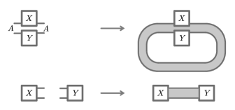
Figure 10: Diagrammatic representation of the Wick contraction rules of the $A$-matrix theory. Physically, the gray shaded areas correspond to ladder series of sequential scatterings off the random Hamiltonian [46].

With these identities, we obtain $\langle\mathrm{str}(P_{\textrm{b}}AA)\rangle_{0}\propto\mathrm{str}(P_{\textrm{b}})\mathrm{str}(\mathds{1})=0$, and so we need to expand the action in its nonlinearity. The first non-vanishing contribution is given by

$$\langle\mathrm{str}(A^{2}P_{\textrm{b}})\rangle\approx\frac{1}{2\cdot 3^{2}}\langle\mathrm{str}(A^{2}P_{\textrm{b}})(\mathrm{str}(A^{3}))^{2}\rangle_{0}=$$

$$\quad=\frac{1}{16\tilde{\epsilon}^{2}},$$

where the above diagrammatic code implies the ’orbit representation’ shown in Fig. 11. Substituting this result into the formula for the spectral density, we obtain

$$\rho(\tilde{\epsilon})\approx\frac{c^{2/3}}{\pi}\left(\tilde{\epsilon}^{1/2}+\frac{1}{32\tilde{\epsilon}^{5/2}}\right)$$

With the identification $\Delta_{0}=c^{2/3}$ this agrees with the expansion Eq. (13). However, we now have a diagrammatic interpretation of the leading order correction in terms of the two-loop diagram shown in Fig. 11, which we will compare to the expansion of the gravitational path integral in section VI.

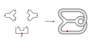
Figure 11: The leading fluctuation diagram modifying the mean field spectral density. Note the torus topology of this diagram: while its representation on a sheet of paper necessarily contains line crossings, a non-crossing representation on a torus is possible. Also note the resemblance to the diagrams of appearing in, e.g., the periodic orbit theory of quantum chaos [47]. However, while these describe the co-propagation of amplitudes of different causality, we here have single self-retracing loops whose existence is tied to the spectral edge.

References

- Haake [2018] F. Haake, Quantum signatures of chaos, 4th edition (Springer-Verlag, Berlin, 2018).
- Efetov [1997] K. B. Efetov, Sypersymmetry in Disorder and Chaos (Cambridge University Press, Cambridge, 1997).
- Mehta [1991] M. L. Mehta, Random matrices (Academic Press, Boston, 1991).
- Saad et al. [2019] P. Saad, S. H. Shenker, and D. Stanford, JT gravity as a matrix integral (2019), arXiv: 1903.11115.
- Note [1] Without entering the subtle question of defining criteria for ‘chaos’, we consider ergodicity of quantum states (in the sense of Ref. [41]) as a necessary condition. Examples of phases ruled out on this basis include (many body) localized, or glassy phases.
- Kitaev [2015] A. Kitaev, A simple model of quantum holography (2015).
- Mertens and Turiaci [2023a] T. G. Mertens and G. J. Turiaci, Solvable models of quantum black holes: a review on Jackiw–Teitelboim gravity, Living Reviews in Relativity 26, 4 (2023a).
- Tracy and Widom [1993] C. A. Tracy and H. Widom, Level-spacing distributions and the Airy kernel, Physics Letters B 305, 115 (1993).
- Note [2] Confusingly, the random matrix community calls such edges ’soft’. However, for us they are ‘hard’ in comparison to the much softer edges of other model systems.
- Kontsevich [1992] M. Kontsevich, Intersection theory on the moduli space of curves and the matrix airy function, Communications in Mathematical Physics 147, 1 (1992).
- García-García and Verbaarschot [2016] A. M. García-García and J. J. M. Verbaarschot, Spectral and thermodynamic properties of the Sachdev-Ye-Kitaev model, Physical Review D 94, 126010 (2016), publisher: American Physical Society.
- García-García and Verbaarschot [2017] A. M. García-García and J. J. Verbaarschot, Analytical spectral density of the Sachdev-Ye-Kitaev model at finite $N$, Physical Review D 96, 066012 (2017), publisher: American Physical Society.
- Altland and Bagrets [2018] A. Altland and D. Bagrets, Quantum ergodicity in the SYK model, Nuclear Physics B 930, 10.1016/j.nuclphysb.2018.02.015 (2018).
- Cotler et al. [2017] J. S. Cotler, G. Gur-Ari, M. Hanada, J. Polchinski, P. Saad, S. H. Shenker, D. Stanford, A. Streicher, and M. Tezuka, Black holes and random matrices, Journal of High Energy Physics 2017, 118 (2017), publisher: Springer Berlin Heidelberg.
- French [1972] J. French, Analysis of distant-neighbor spacing distributions for k-body interaction ensembles, Tech. Rep. (Rochester Univ., NY (USA). Dept. of Physics and Astronomy, 1972).
- Flores et al. [2001] J. Flores, M. Horoi, M. Muller, and T. H. Seligman, Spectral statistics of the two-body random ensemble revisited, Phys. Rev. E 63, 026204 (2001), arXiv:cond-mat/0006144 .
- Altland and Sonner [2021] A. Altland and J. Sonner, Late time physics of holographic quantum chaos, SciPost Physics 11, 034 (2021).
- Note [3] Here, we do not exploit the full symmetry of the solution space to obtain a convergent fluctuation integral [2].
- Berkooz et al. [2019] M. Berkooz, M. Isachenkov, V. Narovlansky, and G. Torrents, Towards a full solution of the large n double-scaled SYK model, Journal of High Energy Physics 2019, 79 (2019).
- French and Wong [1970] J. B. French and S. S. M. Wong, Validity of random matrix theories for many-particle systems, Physics Letters B 33, 449 (1970), publisher: North-Holland.
- Jia and Verbaarschot [2020] Y. Jia and J. J. M. Verbaarschot, Spectral Fluctuations in the Sachdev-Ye-Kitaev Model, JHEP 07, 193, arXiv:1912.11923 [hep-th] .
- [22] H. Gharibyan, M. Hanada, S. H. Shenker, and M. Tezuka, Onset of random matrix behavior in scrambling systems, Journal of High Energy Physics 2018, 124.
- You et al. [2017] Y.-Z. You, A. W. W. Ludwig, and C. Xu, Sachdev-Ye-Kitaev model and thermalization on the boundary of many-body localized fermionic symmetry-protected topological states, Physical Review B 95, 115150 (2017), publisher: American Physical Society.
- [24] That is, the SYK Hamiltonian with Majorana fermions acting on -dimensional Hilbert space of fixed parity.
- Ginsparg and Moore [1993] P. H. Ginsparg and G. W. Moore, Lectures on 2-D gravity and 2-D string theory, in Theoretical Advanced Study Institute (TASI 92): From Black Holes and Strings to Particles (1993) pp. 277–469, arXiv:hep-th/9304011 .
- Note [4] The correspondence is perturbative in that it has been established order by an expansion equivalent to the above -expansion. For its non-perturbative completion in terms of topological string theory, see Ref. [28, 42].
- Mertens and Turiaci [2023b] T. G. Mertens and G. J. Turiaci, Solvable models of quantum black holes: a review on Jackiw–Teitelboim gravity, Living Rev. Rel. 26, 4 (2023b), arXiv:2210.10846 [hep-th] .
- Post et al. [2022] B. Post, J. van der Heijden, and E. Verlinde, A universe field theory for JT gravity, JHEP 05, 118, arXiv:2201.08859 [hep-th] .
- Maldacena [1998] J. M. Maldacena, The Large N limit of superconformal field theories and supergravity, Adv. Theor. Math. Phys. 2, 231 (1998), arXiv:hep-th/9711200 .
- Blommaert et al. [2021] A. Blommaert, T. G. Mertens, and H. Verschelde, Eigenbranes in Jackiw-Teitelboim gravity, JHEP 02, 168, arXiv:1911.11603 [hep-th] .
- Marolf and Maxfield [2020] D. Marolf and H. Maxfield, Transcending the ensemble: baby universes, spacetime wormholes, and the order and disorder of black hole information, JHEP 08, 044, arXiv:2002.08950 [hep-th] .
- Saad et al. [2021] P. Saad, S. H. Shenker, D. Stanford, and S. Yao, Wormholes without averaging (2021), arXiv:2103.16754 [hep-th] .
- Blommaert et al. [2022] A. Blommaert, L. V. Iliesiu, and J. Kruthoff, Gravity factorized, JHEP 09, 080, arXiv:2111.07863 [hep-th] .
- Altland et al. [2023a] A. Altland, B. Post, J. Sonner, J. van der Heijden, and E. P. Verlinde, Quantum chaos in 2D gravity, SciPost Phys. 15, 064 (2023a), arXiv:2204.07583 [hep-th] .
- Belin and de Boer [2021] A. Belin and J. de Boer, Random statistics of OPE coefficients and Euclidean wormholes, Class. Quant. Grav. 38, 164001 (2021), arXiv:2006.05499 [hep-th] .
- Chandra et al. [2022] J. Chandra, S. Collier, T. Hartman, and A. Maloney, Semiclassical 3D gravity as an average of large-c CFTs, JHEP 12, 069, arXiv:2203.06511 [hep-th] .
- Belin et al. [2023] A. Belin, J. de Boer, D. L. Jafferis, P. Nayak, and J. Sonner, Approximate CFTs and Random Tensor Models (2023), arXiv:2308.03829 [hep-th] .
- Eynard [2004] B. Eynard, Topological expansion for the 1-Hermitian matrix model correlation functions, JHEP 11, 031, arXiv:hep-th/0407261 .
- Eynard and Orantin [2007] B. Eynard and N. Orantin, Weil-Petersson volume of moduli spaces, Mirzakhani’s recursion and matrix models (2007), arXiv:0705.3600 [math-ph] .
- Altland et al. [2024] A. Altland, K. W. Kim, T. Micklitz, M. Rezaei, J. Sonner, and J. Verbaarschot, Data and code for ”Quantum chaos on edge” 10.5281/zenodo.10827097 (2024).
- Monteiro et al. [2020] F. Monteiro, M. Tezuka, A. Altland, D. Huse, and T. Micklitz, Quantum ergodicity in the many-body localization problem, arXiv (2020).
- Altland et al. [2023b] A. Altland, B. Post, J. Sonner, J. van der Heijden, and E. P. Verlinde, Quantum chaos in 2d gravity, SciPost Physics 15, 064 (2023b).
- Verbaarschot and Zirnbauer [1984] J. Verbaarschot and M. Zirnbauer, Replica variables, loop expansion, and spectral rigidity of random-matrix ensembles, Annals of Physics 158, 78 (1984).
- Berkooz et al. [2021] M. Berkooz, N. Brukner, V. Narovlansky, and et al., Multi-trace correlators in the syk model and non-geometric wormholes, J. High Energ. Phys. 2021 (196).
- J. Alfaro and Urrutia [1997] R. M. J. Alfaro and L. F. Urrutia, The itzykson-zuber integral for u(m—n), Surveys in High Energy Physics 10, 405 (1997).
- Altland and Simons [2023] A. Altland and B. Simons, Condensed Matter Field Theory (Cambridge University Press, 2023).
- Heusler et al. [2007] S. Heusler, S. Müller, A. Altland, P. Braun, and F. Haake, Periodic-orbit theory of level correlations, Physical Review Letters 98, 10.1103/PhysRevLett.98.044103 (2007).