SPDEs on narrow channels and graphs: convergence and large deviations in case of non smooth noise

Abstract

We investigate a class of stochastic partial differential equations of reaction-diffusion type defined on graphs, which can be derived as the limit of SPDEs on narrow planar channels. In the first part, we demonstrate that this limit can be achieved under less restrictive assumptions on the regularity of the noise, compared to [4]. In the second part, we establish the validity of a large deviation principle for the SPDEs on the narrow channels and on the graphs, as the width of the narrow channels and the intensity of the noise are jointly vanishing.

1 Introduction

In the present paper, we deal with the following stochastic reaction-diffusion equations

$$\begin{dcases}\displaystyle\partial_{t}u_{\epsilon}(t,x,y)=\mathcal{L}_{\epsilon}u_{\epsilon}(t,x,y)+b(u_{\epsilon}(t,x,y))+\partial_{t}w^{Q}(t,x,y),\ \ \ \ (x,y)\in G,\\[10.0pt] \displaystyle\frac{\partial u_{\epsilon}}{\partial\nu_{\epsilon}}(t,x,y)=0,\ \ \ \ (x,y)\in\partial G,\ \ \ \ \ u_{\epsilon}(0,x,y)=u_{0}(x,y),\end{dcases}$$ (1.1)

depending on a small parameter $\epsilon>0$, where

$$\mathcal{L}_{\epsilon}\coloneqq\frac{1}{2}\left(\frac{\partial^{2}}{\partial x^{2}}+\frac{1}{\epsilon^{2}}\frac{\partial^{2}}{\partial y^{2}}\right).$$

Here $G$ is a bounded smooth domain in $\mathbb{R}^{2}$, $\nu_{\epsilon}(x,y)$ is the unit interior co-normal at $\partial G$ associated with $\mathcal{L}_{\epsilon}$, and $w^{Q}(t)$ is a cylindrical Wiener process in $L^{2}(G)$. Under suitable assumptions on the nonlinearity $b$ and the covariance operator $Q$, it can be proved that equation (1.1) is well-posed in $L^{2}(G)$. With the change of variable

$$(x,y)\in\,G\mapsto(x,\epsilon y)\in\,G_{\epsilon}:=\{(x,y)\in\,\mathbb{R}^{2}\,:\,(x,\epsilon^{-1}y)\in\,G\},$$

equation (1.1) can be rewritten as the following stochastic reaction-diffusion equations on the narrow channel $G_{\epsilon}$

$$\begin{dcases}\displaystyle\partial_{t}v_{\epsilon}(t,x,y)=\frac{1}{2}\,\Delta v_{\epsilon}(t,x,y)+b(v_{\epsilon}(t,x,y))+\sqrt{\epsilon}\,\partial_{t}w^{Q_{\epsilon}}(t,x,y),\ \ \ \ (x,y)\in G_{\epsilon},\\[10.0pt] \displaystyle\frac{\partial v_{\epsilon}}{\partial\hat{\nu}_{\epsilon}}(t,x,y)=0,\ \ \ \ (x,y)\in\partial G_{\epsilon},\ \ \ \ \ \ \ \ \ v_{\epsilon}(0,x,y)=u_{0}(x,\epsilon^{-1}y).\end{dcases}$$ (1.2)

Here $\hat{\nu}_{\epsilon}(x,y)$ is the inward unit normal vector at $\partial G_{\epsilon}$ and $Q_{\epsilon}:=R_{\epsilon}\,Q\,R_{\epsilon}^{-1}$, where the operator $R_{\epsilon}:L^{2}(G)\to L^{2}(G_{\epsilon})$ is defined by

$$(R_{\epsilon}f)(x,y):=f(x,y/\epsilon),\ \ \ \ \ f\in\,L^{2}(G),\ \ \ \ (x,y)\in\,G_{\epsilon}.$$

Equations like (1.1) and (1.2) can serve as models for Brownian motors (ratchets) in statistical physics and molecular dynamics in biology, where the particles or molecules move along a designated track which can be viewed as a tubular domain with several wings. See e.g. [12] and [13], as well as [9] for some details about these systems. In recent years there has been a substantial interest in the study of deterministic and stochastic PDEs defined on narrow domains and graphs. However, the existing literature about SPDEs on graphs is relatively limited. In addition to [4], where the limiting behavior of systems like (1.1) and (1.2) has been investigated and suitable SPDEs on graphs have been obtained, we recall [3] and [5], where suitable SPDEs on graphs have been obtained from the fast flow asymptotics of stochastic incompressible planar viscous fluids. Additionally, different viewpoints and approaches to SPDEs on graphs have been explored in works such as [1] and [8].

In the aforementioned paper [4], the first named author and M. Freidlin have studied the limiting behavior of particles/molecules moving in narrow channels with wings, as the width of the channels and wings vanishes, by working directly with equation (1.1). They have shown that $u_{\epsilon}$ converges to the solution of an SPDE defined on the graph $\Gamma$, obtained by identifying all points in the same connected component $C_{k}(x)$ of the cross section

$$C(x):=\{y\in\,\mathbb{R}\ :\ (x,y)\in\,G\}=:\bigcup_{k=1}^{N(x)}C_{k}(x),$$

for all $x\in\,\mathbb{R}$ such that there exists $y\in\,\mathbb{R}$ with $(x,y)\in\,G$ (see Figure 1 and Section 2 for all details). More precisely, for every $g:G\to\mathbb{R}$ they have defined the function $g^{\wedge}:\Gamma\to\mathbb{R}$ by setting

$$g^{\wedge}(x,k):=\frac{1}{l_{k}(x)}\int_{C_{k}(x)}g(x,y)dy,\ \ \ \ \ \ \ \ (x,k)\in\Gamma,$$

and have proved that for every $p\geq 1$ and $0<\tau<T$

$$\lim_{\epsilon\to 0}\mathbb{E}\sup_{t\in\,[\tau,T]}\absolutevalue{u_{\epsilon}(t)-\bar{u}(t)\circ\Pi}_{L^{2}(G)}^{p}=\lim_{\epsilon\to 0}\mathbb{E}\sup_{t\in\,[\tau,T]}\absolutevalue{u_{\epsilon}^{\wedge}(t)-\bar{u}(t)}_{L^{2}(\Gamma,\,\nu)}^{p}=0,$$ (1.3)

where $\Pi$ is the projection of $G$ into $\Gamma$, $\nu$ is a suitable projection on $\Gamma$ of the Lebesgue measure on $G$, that is consistent with the construction of the graph $\Gamma$ (see Subsection 2.3) and $\bar{u}$ is the solution of the stochastic PDE on the graph $\Gamma$

$$\partial_{t}\bar{u}(t)=\bar{L}\bar{u}(t)+b(\bar{u}(t))+\partial_{t}\bar{w}^{Q}(t),\ \ \ \ \ \ \ \ \ \bar{u}(0)=u^{\wedge}_{0}.$$ (1.4)

Here $\bar{w}^{Q}(t)$ is the projection of the cylindrical Wiener process $w^{Q}(t)$ on the graph $\Gamma$, and $\bar{L}$ is the generator of a Markov process $\bar{Z}(t)$ on $\Gamma$, obtained in [11] as the weak limit in $C([0,T];\Gamma)$ of $\Pi(Z_{\epsilon}(t))$, the projection on the graph $\Gamma$ of the diffusion $Z_{\epsilon}(t)$ associated with the operator $\mathcal{L}_{\epsilon}$, endowed with reflecting boundary conditions at $\partial G$.

The process $Z_{\epsilon}(t)$ has a fast vertical component, whose invariant measure is given by the normalized Lebesgue measure, and, as a consequence of an averaging principle, Freidlin and Wentcell proved in [11] that the process $\Pi(Z_{\epsilon}(t))$, that describes the slow component of the motion, converges to the Markov process $\bar{Z}(t)$, as $\epsilon\downarrow 0$. Moreover, they gave an explicit description of the generator $\bar{L}$, in terms of some second order differential operators on each edge of $\Gamma$ and suitable gluing conditions at each internal vertex (see Section 2). Starting from these results, the authors of [4] have studied the limiting behavior of the semigroup $S_{\epsilon}(t)$ associated with the diffusion $Z_{\epsilon}(t)$, and defined as

$$S_{\epsilon}(t)\varphi(z)=\mathbf{E}_{z}\varphi(Z_{\epsilon}(t)),\ \ \ \ \ \ z\in\,G,$$

for every $\varphi:G\to\mathbb{R}$, Borel and bounded. Namely, they have proved that for every $\varphi\in\,L^{2}(G)$ and $0<\tau<T$

$$\lim_{\epsilon\to 0}|S_{\epsilon}(t)\varphi-(\bar{S}(t)\varphi^{\wedge})\circ\Pi|_{L^{2}(G)}=0.$$ (1.5)

Since $u_{\epsilon}$ satisfies the equation

$$u_{\epsilon}(t)=S_{\epsilon}(t)u_{0}+\int_{0}^{t}S_{\epsilon}(t-s)B(u_{\epsilon}(s))ds+w_{\epsilon}(t),\ \ \ \ \ \ \epsilon>0,$$

and $\bar{u}(t)$ satisfies the equation

$$\bar{u}(t)=\bar{S}(t)u_{0}^{\wedge}+\int_{0}^{t}\bar{S}(t-s)B(\bar{u}(s))ds+w_{\bar{L}}(t),$$

where

$$w_{\epsilon}(t):=\int_{0}^{t}S_{\epsilon}(t-s)dw^{Q}(s),\ \ \ \ \ \ \ w_{\bar{L}}(t):=\int_{0}^{t}\bar{S}(t-s)d\bar{w}^{Q}(s),$$

limit (1.5) has allowed them to show that if the noises $w^{Q}(t)$ and $\bar{w}^{Q}(t)$ are regular enough to live in $L^{2}(G)$ and $L^{2}(\Gamma,\nu)$, respectively, then (1.3) holds.

Notice that the assumption that both $w^{Q}(t)$ and $\bar{w}^{Q}(t)$ live in functional spaces was fundamental in [4]. Firstly, the well-posedness of equation (1.4) required that the noise $\bar{w}^{Q}(t)$ was function-valued, as no-smoothing effect of the semigroup $\bar{S}(t)$ was proven. Secondly, and more importantly, limit (1.5) did not allow to prove the convergence of the stochastic convolution $w_{\epsilon}(t)$ to $w_{\bar{L}}(t)$. In the first part of the present paper, we are addressing these problems. In particular, we prove that, under the minimal assumptions on the noise $w^{Q}(t)$ required for the well-posedness of equation (1.1) in the space $L^{2}(G)$, suitable kernel estimates for the semigroup $S_{\epsilon}(t)$ transfer to analogous kernel estimates for $\bar{S}(t)$, allowing us to have the well-posedness of equation (1.4). Moreover, in view of these estimates, we show that limit (1.3) is still valid.

In the second part of the paper, we study the validity of a large deviation principle for equation (1.1) and we show how approximation (1.3) is stable with respect to the small-noise limit. Actually, we fix an arbitrary $\delta>0$ and we consider the equation in $G$

$$\begin{dcases}\displaystyle\partial_{t}u_{\epsilon}(t,x,y)=\mathcal{L}_{\epsilon}u_{\epsilon}(t,x,y)+b(u_{\epsilon}(t,x,y))+\epsilon^{\,\delta/2}\partial_{t}w^{Q}(t,x,y),\ \ \ \ (x,y)\in G,\\[10.0pt] \displaystyle\frac{\partial u_{\epsilon}}{\partial\nu_{\epsilon}}(t,x,y)=0,\ \ \ \ (x,y)\in\partial G,\ \ \ \ \ u_{\epsilon}(0,x,y)=u_{0}(x,y),\end{dcases}$$ (1.6)

or, equivalently, the equation on the narrow channel $G_{\epsilon}$

$$\begin{dcases}\displaystyle\partial_{t}v_{\epsilon}(t,x,y)=\frac{1}{2}\,\Delta v_{\epsilon}(t,x,y)+b(v_{\epsilon}(t,x,y))+\epsilon^{\,(1+\delta)/2}\,\partial_{t}w^{Q_{\epsilon}}(t,x,y),\ \ \ \ (x,y)\in G_{\epsilon},\\[10.0pt] \displaystyle\frac{\partial v_{\epsilon}}{\partial\hat{\nu}_{\epsilon}}(t,x,y)=0,\ \ \ \ (x,y)\in\partial G_{\epsilon},\ \ \ \ \ \ \ \ \ v_{\epsilon}(0,x,y)=u_{0}(x,\epsilon^{-1}y).\end{dcases}$$ (1.7)

Our aim is proving that for every $0<\tau<T$, the family $\{\mathcal{L}(u_{\epsilon})\}_{\epsilon\in\,(0,1)}$ satisfies a large deviation principle in $C([\tau,T];L^{2}(G))$, with speed $\epsilon^{\delta}$ and action functional

$$I_{T}(f)=\frac{1}{2}\,\inf\absolutevalue{\varphi}_{L^{2}(0,T;L^{2}(G))}^{2},$$ (1.8)

where the infimum is taken over all $\varphi\in L^{2}(0,T;L^{2}(G))$ such that $f=(\bar{u}^{\varphi})|_{[\tau,T]}\circ\Pi\in\,C([\tau,T];L^{2}(G))$ and $\bar{u}^{\varphi}$ is the solution to the controlled problem on the graph $\Gamma$

$$\begin{dcases}\displaystyle\partial_{t}\bar{u}^{\varphi}(t,x,k)=\bar{L}\bar{u}^{\varphi}(t,x,k)+b(\bar{u}^{\varphi}(t,x,k))+(Q\varphi)^{\wedge}(t,x,k),\\[10.0pt] \displaystyle\bar{u}^{\varphi}(0,x,k)=u_{0}^{\wedge}(x,k).\end{dcases}$$

In the same way, we obtain that the family $\{\mathcal{L}(u_{\epsilon}^{\wedge})\}_{\epsilon\in\,(0,1)}$ satisfies a large deviation principle in $C([\tau,T];L^{2}(\Gamma,\,\nu))$ with speed $\epsilon^{\delta}$ and action functional $\bar{I}_{T}$, where $\bar{I}_{T}$ is defined as in (1.8), with the infimum taken now over all $\varphi\in L^{2}(0,T;L^{2}(G))$ such that $f=(\bar{u}^{\varphi})|_{[\tau,T]}\in\,C([\tau,T];L^{2}(\Gamma,\,\nu))$. In particular, this means that limit (1.3) is consistent with respect the small-noise limit, in the sense that the large deviation principle for the SPDE on the domain $G$ and, equivalently, on the narrow channel $G_{\epsilon}$, is described by the same large deviation principle that one has for the SPDEs with small noise on the graph.

The paper is organized as follows. In Section 2, we begin by reviewing the assumptions on the domain $G$ and we construct the graph $\Gamma$. We then provide a brief summary of existing results concerning the convergence of $\Pi(Z_{\epsilon})$ to $\bar{Z}$, the convergence of the semigroup $S_{\epsilon}(t)$ to the semigroup $\bar{S}(t)$ and the convergence of the solution of equation (1.1) to the solution of equation (1.4). Section 3 is devoted to the proof of the convergence of the solution of (1.1) to the solution of equation (1.4) under weaker regularity conditions for the noise. In Section 4, we state the large deviation principle result and give an overview of the weak convergence method and introduce the skeleton equation within our specific framework. Finally, in Section 5 and Section 6 we provide the proof of the large deviation principle.

2 Notations and preliminaries

In this section, we present a concise overview of the notations we are going to use throughout the paper and recall some preliminary results from [4] and [11].

2.1 The domain $G$, the narrow channel $G_{\epsilon}$ and the graph $\Gamma$

Let $G$ be a bounded open domain in $\mathbb{R}^{2}$, having a smooth boundary $\partial G$ and satisfying the uniform exterior sphere condition. For any $(x,y)\in\,\partial G$, we denote by $\nu(x,y)$ the unit inward normal vector at the point $(x,y)$.

Now, for every $\epsilon>0$, we introduce the narrow channel $G_{\epsilon}$ associated with $G$

$$G_{\epsilon}\coloneqq\{(x,y)\in\mathbb{R}^{2}:(x,\epsilon^{-1}y)\in G\},$$

and we denote by $\nu^{\epsilon}(x,y)$ the unit inward normal vector at the point $(x,y)\in\partial G_{\epsilon}$. Notice that

$$\nu^{\epsilon}(x,\epsilon y)=c_{\epsilon}(x,y)(\epsilon\nu_{1}(x,y),\nu_{2}(x,y)),\ \ \ (x,y)\in\partial G,$$

for some function $c_{\epsilon}:\partial G\to[1,+\infty)$ such that

$$\sup_{\begin{subarray}{c}x,y\in\partial G\\ \epsilon>0\end{subarray}}c_{\epsilon}(x,y)=c<+\infty.$$

In what follows, we assume that the region $G$ satisfies the following properties

1. There exist only finitely many $x\in\mathbb{R}$ such that $(x,y)\in\partial G$ and $\nu_{2}(x,y)=0$.

2. For every $x\in\mathbb{R}$, the cross-section $C(x)=\{y\in\mathbb{R}:(x,y)\in G\}$ consists of only a finite union of intervals. Namely, when $C(x)\neq\emptyset$, there exist $N(x)\in\mathbb{N}$ and intervals $C_{1}(x),\cdots,C_{N(x)}(x)$ such that

   $$C(x)=\bigcup_{k=1}^{N(x)}C_{k}(x).$$

3. If $x\in\mathbb{R}$ is such that $\nu_{2}(x,y)\neq 0$, then for any $k=1,\cdots,N(x)$ we have

   $$l_{k}(x)=\absolutevalue{C_{k}(x)}>0.$$

By identifying the points within each connected component $C_{k}(x)$ of each cross section $C(x)$, we can construct a graph $\Gamma$. This graph consists of a finite number of vertices $O_{i}$, corresponding to the connected components containing points $(x,y)\in\partial G$ such that $\nu_{2}(x,y)=0$, and with a finite number of edges $I_{k}$, connecting the vertices. On our graph there are two different types of vertices, exterior ones, that are connected to only one edge of the graph, and interior ones, that are connected to two or more edges. See Figure 1.

On the graph $\Gamma$, we can introduce a notion of distance as follows. If $z_{1}=(x_{1},k)$ and $z_{2}=(x_{2},k)$ belong to the same edge $I_{k}$ , then their distance is given by $d(z_{1},z_{2})=\absolutevalue{x_{1}-x_{2}}$. In the case when $z_{1}$ and $z_{2}$ belong to different edges, the distance is determined as

$$d(z_{1},z_{2})=\min\{d(z_{1},O_{i_{1}})+d(O_{i_{1}},O_{i_{2}})+\cdots+d(O_{i_{n}},z_{2})\},$$

where the minimum is taken over all possible paths from $z_{1}$ to $z_{2}$, through every possible sequence of vertices $O_{i_{1}},\cdots,O_{i_{n}}$, that connects $z_{1}$ to $z_{2}$.

Now, any point $z$ on the graph $\Gamma$ can be uniquely characterized by two coordinates: the horizontal coordinate $x$ and the integer $k$ which identifies the edge $I_{k}$ to which $z$ belongs. It is worth noting that if $z$ is an interior vertex $O_{i}$, the second coordinate may not have a unique choice since there are two or more edges having $O_{i}$ as their endpoint.

In the upcoming discussion, we define the mapping $\Pi:G\to\Gamma$ as the identification map that associates points in the domain $G$ to their respective locations on the graph $\Gamma$. For any vertex $O_{i}$ on the graph $\Gamma$, we denote by $E_{i}$ the set $\Pi^{-1}(O_{i})$ consisting of points $(x,y)\in\partial G$ such that $\nu_{2}(x,y)=0$. The set $E_{i}$ can be one point, several points or an interval. Henceforth, we assume that $G$ satisfies the following condition:

1. For each vertex $O_{i}$, either $\nu_{1}(x,y)>0$, for all $(x,y)\in E_{i}$, or $\nu_{1}(x,y)<0$, for all $(x,y)\in E_{i}$.

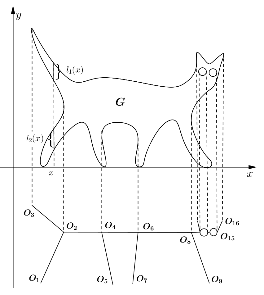
Figure 1: The domain $G$ and the graph $\Gamma$

2.2 Limiting results for the transition semigroup

In order to understand the limiting behavior of the differential operator $\mathcal{L}_{\epsilon}$, endowed with the Neumann boundary condition, and its associated semigroup $S_{\epsilon}(t)$, we consider the following stochastic differential equation with reflecting boundary conditions on the domain $G$

$$\begin{dcases}\displaystyle dX^{\epsilon}=dB_{1}(t)+\nu_{1}(X^{\epsilon}(t),Y^{\epsilon}(t))d\phi^{\epsilon}(t),\ \ \ \ X^{\epsilon}(0)=x,\\[10.0pt] \displaystyle dY^{\epsilon}=\frac{1}{\epsilon}\,dB_{2}(t)+\frac{1}{\epsilon^{2}}\,\nu_{2}(X^{\epsilon}(t),Y^{\epsilon}(t))\,d\phi^{\epsilon}(t),\ \ \ \ Y^{\epsilon}(0)=y,\end{dcases}$$ (2.1)

where $(x,y)\in G$. Such an equation can be rewritten as

$$dZ^{\epsilon}(t)=\sqrt{\sigma_{\epsilon}}\,dB(t)+\sigma_{\epsilon}\,\nu(Z^{\epsilon}(t))\,d\phi^{\epsilon}(t),\ \ \ \ Z^{\epsilon}(0)=z,$$

where $z=(x,y)\in G$ and

$$\sigma_{\epsilon}=\begin{pmatrix}1&0\\ 0&\epsilon^{-2}\end{pmatrix}.$$

Here $B(t)=(B_{1}(t),B_{2}(t))$ is a $2$-dimensional Brownian motion defined on a stochastic basis $(\mathbf{\Omega},\mathbf{\mathcal{F}},\{\mathbf{\mathcal{F}}\}_{t\geq 0},\mathbf{P})$ and $\phi^{\epsilon}(t)$ is the local time of the process $Z^{\epsilon}(t)$ on the boundary $\partial G$. That is, $\phi^{\epsilon}(t)$ is an adapted process, continuous with probability 1, non-decreasing and increasing only when $Z^{\epsilon}(t)\in\partial G$. Formally, one can write

$$\phi^{\epsilon}(t)=\int_{0}^{t}I_{\{Z^{\epsilon}(s)\in\partial G\}}d\phi^{\epsilon}(s).$$

One can show that the generator of $Z^{\epsilon}$ is $\mathcal{L}_{\epsilon}$, endowed with Neumann boundary conditions.

In [11], a continuous Markov process $\bar{Z}(t)$ on $\Gamma$ is introduced. Its generator $\bar{L}$ is given by suitable differential operators $\bar{\mathcal{L}}_{k}$ within each edge $I_{k}=\{(x,k):a_{k}\leq x\leq b_{k}\}$ of the graph and is subject to certain gluing conditions at the vertices $O_{i}$. More precisely, for each $k$ the differential operator $\bar{\mathcal{L}}_{k}$ has the form

$$\bar{\mathcal{L}}_{k}f(x)=\frac{1}{2l_{k}(x)}\frac{d}{dx}\left(l_{k}\frac{df}{dx}\right)(x),\ \ \ a_{k}<x<b_{k},$$ (2.2)

and the operator $\bar{L}$, acting on functions $f$ defined on the graph $\Gamma$, is defined as

$$\bar{L}f(x,k)=\bar{\mathcal{L}}_{k}f(x),\ \ \ \text{if $(x,k)$ is an interior point of $I_{k}$}.$$

The domain $D(\bar{L})$ is defined as the set of continuous functions on the graph $\Gamma$, that are twice continuously differentiable in the interior part of each edge, such that for any vertex $O_{i}=(x_{i},k_{i,1})=\cdots=(x_{i},k_{i,n_{i}})$ there exists finite

$$\lim_{(x,k_{i,j})\to O_{i}}\bar{L}f(x,k_{i,j}).$$

Moreover, the following one-sided limits exist

$$\lim_{x\to x_{i}}l_{k_{i,j}}(x)\frac{df}{dx}(x,k_{i,j})$$

along any edge $I_{k_{i,j}}$ ending at the vertex $O_{i}=(x_{i},k_{i,j})$ and the following gluing condition at each vertex $O_{i}$ is satisfied

$$\sum_{k:I_{k}\sim O_{i}}\lim_{x\to x_{i}}\left(\pm l_{k}(x)\frac{df}{dx}(x,k)\right)=0,$$ (2.3)

where the sign $+$ is taken for right limits and the sign $-$ for left limits. In the case of an exterior vertex $O_{i}$, the gluing condition (2.3) reduces to

$$\lim_{x\to x_{i}}l_{k}(x)\frac{df}{dx}(x,k)=0,$$ (2.4)

along the only edge $I_{k}$ terminating at $O_{i}$.

In what follows, the transition semigroup associated with the process $\bar{Z}(t)$ is denoted by $\bar{S}(t)$. In other words, for any Borel and bounded function $f:\Gamma\to\mathbb{R}$, we have

$$\bar{S}(t)f(x,k)=\bar{\mathbf{E}}_{(x,k)}f(\bar{Z}(t)),$$

where $\bar{\mathbf{E}}_{x,k}$ is the expectation associated with the Markov process $\bar{Z}(t)$ starting at $(x,k)\in\Gamma$.

In [11] the convergence in distribution of the non-Markov process $\Pi(Z_{\epsilon}(t))$, which characterizes the slow motion of the process, to the Markov process $\bar{Z}(t)$ in the space $C([0,T];\Gamma)$ is proven.

Theorem 2.1.

[11, Theorem 1.2] For any bounded and continuous functional $F$ on $C([0,T];\Gamma)$ and $z\in G$ it holds

$$\lim_{\epsilon\to 0}\mathbf{E}_{z}F(\Pi(Z^{\epsilon}(\cdot)))=\bar{\mathbf{E}}_{\Pi(z)}F(\bar{Z}(\cdot)).$$

2.3 Functions and operators on the graph $\Gamma$

In this subsection, we recall the basic definitions of functions and operators defined on $G$ and $\Gamma$, as introduced in [4], as well as some convergences results which we will use in what follows.

We denote by $H$ the Hilbert space $L^{2}(G)$, endowed with the scalar product $\langle\cdot,\cdot\rangle_{H}$ and the corresponding norm $|\cdot|_{H}$. Moreover, we denote by $H^{1}$ the classical Sobolev space $W^{1,2}(G)$, endowed with the norm

$$\absolutevalue{f}_{H^{1}}\coloneqq\absolutevalue{f}_{H}+\absolutevalue{\nabla f}_{H}.$$

Now we denote by $\bar{H}$ the space of measurable functions $f:\Gamma\to\mathbb{R}$ such that

$$\sum_{k=1}^{N}\int_{I_{k}}\absolutevalue{f(x,k)}^{2}l_{k}(x)dx<+\infty$$

(here $N$ is the total number of edges of $\Gamma$). The space $\bar{H}$ is a Hilbert space once endowed with the inner product

$$\langle f,g\rangle_{\bar{H}}=\sum_{k=1}^{N}\int_{I_{k}}f(x,k)g(x,k)l_{k}(x)dx.$$

Note that if we introduce in $\Gamma$ the measure $\nu$

$$\nu(A):=\sum_{k=1}^{N}\int_{I_{k}}I_{A}(x,k)l_{k}(x)dx,\ \ \ A\in\mathcal{B}(\Gamma),$$ (2.5)

we have that $\bar{H}=L^{2}(\Gamma,\nu)$.

Now, for any $u\in H$ we define

$$u^{\wedge}(x,k):=\frac{1}{l_{k}(x)}\int_{C_{k}(x)}u(x,y)dy,\ \ \ \ \ \ \ \ (x,k)\in\Gamma,$$

and for any $f\in\bar{H}$ we define

$$f^{\vee}(x,y):=f(\Pi(x,y)),\ \ \ \ \ \ \ \ (x,y)\in G.$$

Moreover, for any $Q\in\mathcal{L}(H)$ and $f\in\bar{H}$, we define

$$Q^{\wedge}f:=\left(Qf^{\vee}\right)^{\wedge},$$

and, similarly, for any $A\in\mathcal{L}(\bar{H})$ and $u\in H$, we define

$$A^{\vee}u:=\left(Au^{\wedge}\right)^{\vee}.$$

Below, we summarize some properties which can be derived from the aforementioned definitions.

Proposition 2.2.

[4] For every $u\in H$ and $f\in\bar{H}$ we have

$$\langle u^{\wedge},f\rangle_{\bar{H}}=\langle u,f^{\vee}\rangle_{H},\ \ \ \ \ (f^{\vee})^{\wedge}=f.$$ (2.6)

In particular, if $\{f_{n}\}_{n\in\mathbb{N}}$ is an orthonormal basis in $\bar{H}$, then $\{f_{n}^{\vee}\}_{n\in\mathbb{N}}$ is an orthonormal basis in $H$. Moreover,

$$\|f^{\vee}\|_{H}=\|f\|_{\bar{H}},\ \ \ \ \ \ \ \|u^{\wedge}\|_{\bar{H}}\leq\|u\|_{H}.$$

Next, for every $Q\in\mathcal{L}(H)$ and $A\in\mathcal{L}(\bar{H})$ we have

$$\lVert Q^{\wedge}\rVert_{\mathcal{L}(\bar{H})}\leq\lVert Q\rVert_{\mathcal{L}(H)},$$

and

$$\lVert A^{\vee}\rVert_{\mathcal{L}(H)}\leq\lVert A\rVert_{\mathcal{L}(\bar{H})},\ \ \ \ \ \ \ \ \left(A^{\vee}\right)^{\wedge}=A.$$ (2.7)

Finally, if $Q\in\mathcal{L}_{2}(H)$, we have

$$\lVert Q^{\wedge}\rVert_{\mathcal{L}_{2}(\bar{H})}\leq\lVert Q\rVert_{\mathcal{L}_{2}(H)}.$$

Once introduced all these notations, we can state the convergence result of the semigroup $S_{\epsilon}(t)$ to the semigroup $\bar{S}(t)$.

Theorem 2.3.

[4, Corollary 5.3 and Theorem 5.4] For any $0<\tau<T$, $\varphi\in C(\bar{G})$ and $z\in G$, we have

$$\lim_{\epsilon\to 0}\,\sup_{t\in[\tau,T]}\absolutevalue{S_{\epsilon}(t)\varphi(z)-\bar{S}(t)^{\vee}\varphi(z)}=0.$$

For every $\varphi\in H$ it holds

$$\lim_{\epsilon\to 0}\,\sup_{t\in[\tau,T]}\absolutevalue{S_{\epsilon}(t)\varphi-\bar{S}(t)^{\vee}\varphi}_{H}=\lim_{\epsilon\to 0}\,\sup_{t\in[\tau,T]}\absolutevalue{(S_{\epsilon}(t)\varphi)^{\wedge}-\bar{S}(t)\varphi^{\wedge}}_{\bar{H}}=0.$$

Moreover, $\bar{S}(t)$ extends to a contraction semigroup on $\bar{H}$.

2.4 Limiting results for the SPDE on $G$

We recall that $G\subset\mathbb{R}^{2}$ is a bounded open set with regular boundary. In what follows, we shall assume the following conditions.

Hypothesis 1.

The nonlinearity $b:\mathbb{R}\to\mathbb{R}$ is Lipschitz continuous.

In particular, this means that

$$B:H\to H,\ \ \ u\in H\mapsto B(u):=b\circ u\in H$$

is well-defined and Lipschitz continuous. Similarly, we have that $B:\bar{H}\to\bar{H}$ is well defined and Lipschitz continuous. Moreover, it is immediate to check that for every $f\in\,\bar{H}$

$$B(f^{\vee})=(B(f))^{\vee}.$$ (2.8)

We fix a bounded linear operator $Q$ in $H$ such that

$$Qe_{k}=\lambda_{k}e_{k}$$ (2.9)

for some orthonormal basis $\{e_{k}\}_{k\in\mathbb{N}}$ in $H$ and some sequence $\{\lambda_{k}\}_{k\in\mathbb{N}}\subset[0,\infty)$, and we assume that $w^{Q}(t)$ is a cylindrical Wiener process with covariance $Q^{2}$. This means that it can be written as

$$w^{Q}(t)=\sum_{k=1}^{\infty}\lambda_{k}e_{k}\beta_{k}(t),$$

where $\{\beta_{k}(t)\}_{k\in\mathbb{N}}$ is a sequence of mutually independent Brownian motions defined on some stochastic basis $(\Omega,\mathcal{F},\{\mathcal{F}_{t}\},\mathbb{P},\mathbb{E})$.

In [4], it is assumed that the series above converges in $L^{2}(\Omega;H)$. Namely, the following stronger condition on the operator $Q$ is assumed

$$\lVert Q\rVert_{\mathcal{L}_{2}(H)}^{2}=\sum_{k=1}^{\infty}\absolutevalue{Qe_{k}}_{H}^{2}=\sum_{k=1}^{\infty}\lambda_{k}^{2}<+\infty.$$ (2.10)

Under these assumptions (but in fact, weaker conditions on $w^{Q}$ can be assumed, see section 3 for more detail), for any $\epsilon>0$ equation (1.1) admits a unique mild solution $u_{\epsilon}$ in $L^{p}(\Omega,C([0,T];H))$ (see e.g. [6]). More precisely, for any $T>0$ and $p\geq 1$, there exists a unique adapted process $u_{\epsilon}\in L^{p}(\Omega,C([0,T];H))$ such that

$$u_{\epsilon}(t)=S_{\epsilon}(t)u_{0}+\int_{0}^{t}S_{\epsilon}(t-s)B(u_{\epsilon}(s))ds+\int_{0}^{t}S_{\epsilon}(t-s)dw^{Q}(s).$$

In addition, the process

$$\bar{w}^{Q}(t)\coloneqq w^{Q}(t)^{\wedge}=\sum_{k=1}^{\infty}(Qe_{k})^{\wedge}\beta_{k}(t)=\sum_{k=1}^{\infty}\lambda_{k}\,e_{k}^{\wedge}\,\beta_{k}(t),\ \ \ \ t\geq 0,$$

is well-defined in $L^{2}(\Omega,\bar{H})$. This, together with the fact that $\bar{S}(t)$ is a contraction semigroup on $\bar{H}$, implies that equation (1.4) is well-posed in $L^{p}(\Omega,C([0,T];\bar{H}))$ and the solution $\bar{u}(t)$ satisfies the equation

$$\bar{u}(t)=\bar{S}(t)u_{0}^{\wedge}+\int_{0}^{t}\bar{S}(t-s)B(\bar{u}(s))ds+\int_{0}^{t}\bar{S}(t-s)d\bar{w}^{Q}(s).$$

As we mentioned in the Introduction, in [4] it has been proved that the solution to (1.1) converges to the solution to (1.4). More precisely

Theorem 2.4.

[4, Theorem 7.2] For every $u_{0}\in\,H$, $p\geq 1$ and $T>0$, and for every $\tau\in\,(0,T)$ we have

$$\lim_{\epsilon\to 0}\,\mathbb{E}\sup_{t\in[\tau,T]}\absolutevalue{u_{\epsilon}(t)-\bar{u}(t)^{\vee}}_{H}^{p}=\lim_{\epsilon\to 0}\,\mathbb{E}\sup_{t\in[\tau,T]}\absolutevalue{u_{\epsilon}(t)^{\wedge}-\bar{u}(t)}_{\bar{H}}^{p}=0.$$ (2.11)

3 Convergence of solutions in case of rough noise

In this section we show that Theorem 2.4 holds under a condition on the regularity of the noise that is considerably weaker than (2.10). We recall that since $Q\in\,\mathcal{L}^{+}(H)$ there exists a complete orthonormal system $\{e_{k}\}_{k\in\,\mathbb{N}}$ in $H$ and a sequence $\{\lambda_{k}\}_{k\in\,\mathbb{N}}\subset[0,+\infty)$ such that $Qe_{k}=\lambda_{k}e_{k}$. In what follows, we shall assume that the eigenvalues $\lambda_{k}$ satisfy the following condition.

Hypothesis 2.

There exists $r<\infty$ such that

$$\kappa_{Q,r}:=\sum_{k=1}^{\infty}\lambda_{k}^{r}<+\infty.$$

Note that, since we are not assuming that $r=2$, the cylindrical Wiener process $w^{Q}(t)$ is not well-defined in $H$. In fact, $w^{Q}(t)$ lives in some larger space Hilbert $U\supset H$ such that the embedding $U_{0}\coloneqq Q(H)\xhookrightarrow{}U$ is Hilbert-Schmidt. Similarly,

$$\bar{w}^{Q}(t)=\sum_{k=1}^{\infty}\lambda_{k}\,e_{k}^{\wedge}\,\beta_{k}(t)$$

is not well-defined in $\bar{H}$ but lives in some larger space $\bar{U}\supset\bar{H}$ with the Hilbert-Schmidt embedding $\bar{U}_{0}\coloneqq Q^{\wedge}(\bar{H})\xhookrightarrow{}\bar{U}$ (see e.g. [6] for more detail). Moreover, Hypothesis 2 is the necessary assumption to ensure the well-posedness of the classical stochastic heat equation in dimension $d=2$.

Theorem 3.1.

Under Hypotheses 1 and 2, for any $u_{0}\in H$, $p\geq 1$, and $0<\tau<T$, it holds

$$\lim_{\epsilon\to 0}\,\mathbb{E}\sup_{t\in[\tau,T]}\absolutevalue{u_{\epsilon}(t)-\bar{u}(t)^{\vee}}_{H}^{p}=\lim_{\epsilon\to 0}\,\mathbb{E}\sup_{t\in[\tau,T]}\absolutevalue{u_{\epsilon}(t)^{\wedge}-\bar{u}(t)}_{\bar{H}}^{p}=0.$$ (3.1)

We have

$$u_{\epsilon}(t) -\bar{u}(t)^{\vee}=S_{\epsilon}(t)u_{0}-\bar{S}(t)^{\vee}u_{0}$$

$$+\int_{0}^{t}\left(S_{\epsilon}(t-s)B(u_{\epsilon}(s))-\bar{S}(t)^{\vee}B(\bar{u}(s))\right)\,ds+w_{\epsilon}(t)-w_{\bar{L}}(t)^{\vee},$$

where

$$w_{\epsilon}(t):=\int_{0}^{t}S_{\epsilon}(t-s)\,dw^{Q}(s),\ \ \ \ \ \ \ w_{\bar{L}}(t):=\int_{0}^{t}\bar{S}(t-s)\,d\bar{w}^{Q}(s).$$ (3.2)

Thanks to Theorem 2.3, we can proceed as in [4, Proof of Theorem 7.2] and we have that (3.1) follows once we show that

$$\lim_{\epsilon\to 0}\mathbb{E}\,\sup_{t\in\,[0,T]}|w_{\epsilon}(t)-w_{\bar{L}}(t)^{\vee}|_{H}^{p}=0.$$ (3.3)

3.1 Proof of (3.3)

In order to prove (3.3), we will need some preliminary results.

Lemma 3.2.

Under Hypothesis 2, for all $T>0$ we have

$$\sup_{\epsilon\in\,(0,1)}\|S_{\epsilon}(s)\|^{2}_{\mathcal{L}_{2}(U_{0},H)}=\sup_{\epsilon\in\,(0,1)}\,\sum_{k=1}^{\infty}\absolutevalue{S_{\epsilon}(s)Qe_{k}}_{H}^{2}\leq c_{T}\,\kappa_{Q,r}^{2/r}\,s^{-\frac{r-2}{r}},\ \ \ \ s\in\,(0,T].$$ (3.4)

Moreover, for every $\eta>0$ there exists $N_{\eta}\in\,\mathbb{N}$ such that

$$\sup_{\epsilon\in\,(0,1)}\,\sum_{k\geq N_{\eta}}\absolutevalue{S_{\epsilon}(s)Qe_{k}}_{H}^{2}\leq\eta\,s^{-\frac{r-2}{r}},\ \ \ \ s\in\,(0,T].$$ (3.5)

Proof.

By Hölder inequality we have

$$\sum_{k=1}^{\infty}\absolutevalue{S_{\epsilon}(s)Qe_{k}}_{H}^{2}=\sum_{k=1}^{\infty}\lambda_{k}^{2}\absolutevalue{S_{\epsilon}(s)e_{k}}_{H}^{2}\leq\kappa_{Q,r}^{2/r}\left(\,\sum_{k=1}^{\infty}\absolutevalue{S_{\epsilon}(s)e_{k}}_{H}^{\frac{2r}{r-2}}\right)^{\frac{r-2}{r}}=\kappa_{Q,r}^{2/r}\,J_{\epsilon}(s)^{\frac{r-2}{r}},$$ (3.6)

where

$$J_{\epsilon}(s)\coloneqq\sum_{k=1}^{\infty}\absolutevalue{S_{\epsilon}(s)e_{k}}_{H}^{\frac{2r}{r-2}}=\sum_{k=1}^{\infty}\absolutevalue{S_{\epsilon}(s)e_{k}}_{H}^{2}\absolutevalue{S_{\epsilon}(s)e_{k}}_{H}^{\frac{4}{r-2}}\leq\sum_{k=1}^{\infty}\absolutevalue{S_{\epsilon}(s)e_{k}}_{H}^{2}$$

(last inequality is due to the fact that $S_{\epsilon}(t)$ is a contraction semigroup on $H$ and $\{e_{k}\}$ is an orthonormal basis for $H$).

Now, for any $z=(x,y),z^{\prime}=(x^{\prime},y^{\prime})\in G$, we denote by $K_{\epsilon}(s,z,z^{\prime})$ the heat kernel of the semigroup $S_{\epsilon}(s)$. Namely

$$S_{\epsilon}(s)u_{0}(z)=\int_{G}K_{\epsilon}(s,z,z^{\prime})u_{0}(z^{\prime})dz^{\prime}=\langle K_{\epsilon}(s,z,\cdot),u_{0}\rangle_{H},\ \ \ \ \ \ \ u_{0}\in H,\ \ \ z\in\,G.$$

According to [7, Theorem 3.2.9], the following heat kernel estimate holds

$$K_{\epsilon}(t,z,z^{\prime})\leq\frac{c_{T}}{t}\exp{\left(-\frac{\epsilon^{2}\left(\absolutevalue{x-x^{\prime}}^{2}+\absolutevalue{y-y^{\prime}}^{2}\right)}{c\,t}\right)}\leq\frac{c_{T}}{t},\ \ \ \ \ t\in\,[0,T]$$ (3.7)

for some $c,c_{T}>0$. This allows to conclude that

$$J_{\epsilon}(s)\leq\sum_{k=1}^{\infty}\absolutevalue{S_{\epsilon}(s)e_{k}}_{H}^{2}=\sum_{k=1}^{\infty}\int_{G}|\langle K_{\epsilon}(s,z,\cdot),e_{k}\rangle_{H}|^{2}\,dz=\int_{G}|K_{\epsilon}(s,z,\cdot)|_{H}^{2}\,dz\leq\frac{c_{T,G}}{s}.$$

In particular, due to (3.6), this implies (3.4).

Now, for every $N\in\,\mathbb{N}$, we have

$$\sum_{k\geq N} \absolutevalue{S_{\epsilon}(s)Qe_{k}}_{H}^{2}=\sum_{k\geq N}\lambda_{k}^{2}\absolutevalue{S_{\epsilon}(s)e_{k}}_{H}^{2}$$

$$\leq\left(\,\sum_{k\geq N}\lambda_{k}^{r}\right)^{2/r}\left(\,\sum_{k=1}^{\infty}\absolutevalue{S_{\epsilon}(s)e_{k}}_{H}^{\frac{2r}{r-2}}\right)^{\frac{r-2}{r}}=\left(\,\sum_{k\geq N}\lambda_{k}^{r}\right)^{2/r}\,J_{\epsilon}(s)^{\frac{r-2}{r}},$$

so that, for every $\epsilon\in\,(0,1)$, we get

$$\sum_{k\geq N}\absolutevalue{S_{\epsilon}(s)Qe_{k}}_{H}^{2}\leq c_{T}\,\left(\,\sum_{k\geq N}\lambda_{k}^{r}\right)^{2/r}s^{-\frac{r-2}{2}},\ \ \ \ \ s\in\,(0,T],$$

As a consequence of Hypothesis 2, this implies that for every $\eta>0$ we can find $N_{\eta}\in\,\mathbb{N}$ such that (3.5) holds.

∎

Next, we want to prove an analogous of Lemma 3.2 for $\bar{S}(t)^{\vee}$.

Remark 3.3.

In order to prove a result analogous to Lemma 3.2 for $\bar{S}(t)^{\vee}$, one should first show that $\bar{S}(t)^{\vee}$ admits a kernel and an estimate analogous to (3.7) holds for $\bar{S}(t)^{\vee}$. There are two possible approaches to obtain this kind of results.

1. On the one hand, Theorem 2.3 implies that $K_{\epsilon}(t,z,\cdot)$ converges to some $\hat{K}(t,z,\cdot)$ weakly, as $\epsilon\downarrow 0$, for every $t>0$ and $z\in\,G$, and the limit $\hat{K}(s,z,z^{\prime})$ is a kernel for $\bar{S}(t)^{\vee}$. Namely

   $$\bar{S}^{\vee}(t)u_{0}(z)=\int_{G}\hat{K}(t,z,z^{\prime})u_{0}(z^{\prime})dz^{\prime}=\langle\bar{K}(t,z,\cdot),u_{0}\rangle_{H},\ \ \ \ \ \ u_{0}\in\,H.$$

   As a result, the uniform heat kernel estimate (3.7) remains valid for $\hat{K}(t,z,z^{\prime})$, that is

   $$\hat{K}(t,z,z^{\prime})\leq\frac{c_{T}}{t},\ \ \ \ \ t\in\,(0,T].$$ (3.8)

2. On the other hand, one could work directly with the semigroup $\bar{S}(t)$ on the graph $\Gamma$ and show that it admits a kernel $\bar{K}(t,x,x^{\prime})$. In this regard, $\bar{K}$ would be a one-dimensional heat kernel and one can expect that the following bound

   $$\bar{K}(s,x,x^{\prime})\leq\frac{c}{s^{1/2}}\exp\left(-\frac{d(x,x^{\prime})^{2}}{c\,s}\right)$$ (3.9)

   should be satisfied. Such a result can be achieved by checking the volume doubling property and the Poincaré inequality, which would allow to get the two-sided heat kernel estimate thanks to the result in [14]. Alternatively, one could utilize the result in [8] by recognizing that the Dirichlet form

   $$\mathcal{E}(f,g)\coloneqq\langle-\bar{L}f,g\rangle_{\bar{H}}$$

   fits into their setting. Another approach could be to use the analysis of the transition probability in [10] to achieve the desired order $s^{-\frac{1}{2}}$.

However, for the purpose of this paper bound (3.8) is sufficient and we will not address bound (3.9).

Lemma 3.4.

If Hypothesis 2 holds for some $r\in(2,\infty)$, then there exists $c_{T}>0$ such that

$$\|\bar{S}^{\vee}(s)\|^{2}_{\mathcal{L}_{2}(U_{0},H)}=\sum_{k=1}^{\infty}\absolutevalue{\bar{S}^{\vee}(s)Qe_{k}}_{H}^{2}\leq c_{T}\,\kappa_{Q,r}^{2/r}\,s^{-\frac{r-2}{r}},\ \ \ \ \ \ \ s\in(0,T].$$ (3.10)

Moreover, for every $\eta>0$ there exists $N_{\eta}\in\,\mathbb{N}$ such that

$$\sum_{k\geq N_{\eta}}\absolutevalue{\bar{S}(s)^{\vee}Qe_{k}}_{H}^{2}\leq\eta\,s^{-\frac{r-2}{r}},\ \ \ \ s\in\,(0,T].$$ (3.11)

Proof.

The family $\bar{S}(t)^{\vee}$, $t\geq 0$, defines a semigroup of bounded linear operators in $H$. Actually, due to (2.6), for every $t,s\geq 0$ and $g\in\,H$ we have

$$\bar{S}(t+s)^{\vee}g =\left(\bar{S}(t+s)g^{\wedge}\right)^{\vee}=\left(\bar{S}(t)\bar{S}(s)g^{\wedge}\right)^{\vee}=\left(\bar{S}(t)((\bar{S}(s)g^{\wedge})^{\vee})^{\wedge}\right)^{\vee}$$

$$=\left(\bar{S}(t)(\bar{S}(s)^{\vee}g)^{\wedge}\right)^{\vee}=\bar{S}(t)^{\vee}(\bar{S}(s)^{\vee}g).$$

Moreover, since $\bar{S}(t)$ is a contraction, due to (2.7) we have that $\bar{S}(t)^{\vee}$ is also a contraction.

Therefore, since $\bar{S}(t)^{\vee}$ is a semigroup of contractions in $H$ and (3.8) holds, the proof is the same as the one in Lemma 3.2. ∎

As a consequence of Lemma 3.2 and Lemma 3.4, we have the following bounds.

Lemma 3.5.

Under Hypothesis 2, there exists some $\alpha\in(0,\frac{1}{2})$ such that

$$\sup_{\epsilon\in\,(0,1)}\,\int_{0}^{T}s^{-2\alpha}\lVert S_{\epsilon}(s)\rVert_{\mathcal{L}_{2}(U_{0};H)}^{2}ds<+\infty,$$ (3.12)

and

$$\int_{0}^{T}s^{-2\alpha}\lVert\bar{S}^{\vee}(s)\rVert_{\mathcal{L}_{2}(U_{0};H)}^{2}ds<+\infty.$$ (3.13)

Moreover

$$\lim_{\epsilon\to 0}\int_{0}^{T}\lVert S_{\epsilon}(s)-\bar{S}^{\vee}(s)\rVert_{\mathcal{L}_{2}(U_{0};H)}^{2}ds=0.$$ (3.14)

Proof.

In view of Lemma 3.2,

$$\int_{0}^{T}s^{-2\alpha}\lVert S_{\epsilon}(s) \rVert_{\mathcal{L}_{2}(U_{0};H)}^{2}ds=\sum_{k=1}^{\infty}\int_{0}^{T}s^{-2\alpha}\absolutevalue{S_{\epsilon}(s)Qe_{k}}_{H}^{2}ds\leq c_{T}\,\kappa_{Q,r}^{2/r}\int_{0}^{T}s^{-2\alpha}s^{-\frac{r-2}{r}}ds.$$

The integral is above is finite if and only if

$$2\alpha+\frac{r-2}{r}=1-2(1/r-\alpha)<1.$$

Thus, if we pick $\alpha\in\left(0,\frac{1}{r}\right)$ we obtain (3.12). In the same way, due to (3.10), we obtain (3.13).

Finally, let us prove (3.14). Since both $S_{\epsilon}(t)$ and $\bar{S}(t)^{\vee}$ are contractions, for every $N\in\,\mathbb{N}$ we have

$$\lVert S_{\epsilon}(s) -\bar{S}^{\vee}(s)\rVert_{\mathcal{L}_{2}(U_{0};H)}^{2}=\sum_{k\leq N}\lambda_{k}^{2}|(S_{\epsilon}(s)-\bar{S}^{\vee}(s))e_{k}|_{H}^{2}+\sum_{k>N}\lambda_{k}^{2}|(S_{\epsilon}(s)-\bar{S}^{\vee}(s))e_{k}|_{H}^{2}$$

$$\leq\|Q\|^{2}_{\mathcal{L}(H)}\sum_{k\leq N}|(S_{\epsilon}(s)-\bar{S}^{\vee}(s))e_{k}|_{H}^{2}+c\,\left(\,\sum_{k>N}\lambda_{k}^{r}\right)^{\frac{2}{r}}\left(\,\sum_{k>N}|(S_{\epsilon}(s)-\bar{S}^{\vee}(s))e_{k}|_{H}^{2}\right)^{\frac{r}{r-2}}$$

By proceeding as in the proofs of Lemma 3.2 and Lemma 3.4, we have

$$\sum_{k>N}|(S_{\epsilon}(s)-\bar{S}^{\vee}(s))e_{k}|_{H}^{2}\leq c_{T}\,s^{-1}.$$

Moreover, due to Hypothesis 2, for every $\eta>0$ we can find $N_{\eta}\in\,\mathbb{N}$ such that

$$\left(\,\sum_{k>N_{\eta}}\lambda_{k}^{r}\right)^{\frac{2}{r}}\leq\eta.$$

Thus, we get

$$\int_{0}^{T}\lVert S_{\epsilon}(s)-\bar{S}^{\vee}(s)\rVert_{\mathcal{L}_{2}(U_{0};H)}^{2}\,ds\leq c\sum_{k\leq N_{\eta}}\int_{0}^{T}|(S_{\epsilon}(s)-\bar{S}^{\vee}(s))e_{k}|_{H}^{2}\,ds+c_{T}\,\eta\int_{0}^{T}s^{-\frac{r}{r-2}}\,ds.$$

According to Theorem 2.3 and the Dominated Convergence theorem, we have

$$\lim_{\epsilon\to 0}\sum_{k\leq N_{\eta}}\int_{0}^{T}|(S_{\epsilon}(s)-\bar{S}^{\vee}(s))e_{k}|_{H}^{2}\,ds=0,$$

and then, due to the arbitrariness of $\eta>0$, we obtain (3.14).

∎

Remark 3.6.

As a consequence of (3.12) and (3.13), for every $T>0$, $p\geq 1$ and $\epsilon>0$ we obtain the well-posedness in $L^{p}(\Omega;C([0,T];H))$ for equation (1.1) and the well-posedness in $L^{p}(\Omega;C(0,T;\bar{H}))$ for equation (1.4).

Now, we can prove (3.3). Let $\alpha\in(0,\frac{1}{2})$ as in Lemma 3.5. From the stochastic factorization formula we get that for any $t\in[0,T]$

$$\frac{\pi}{\sin\pi\alpha}(w_{\epsilon}(t)-w_{\bar{L}}(t)^{\vee})=\int_{0}^{t} (t-s)^{\alpha-1}S_{\epsilon}(t-s)Y_{\alpha,1}^{\epsilon}(s)ds$$

$$+\int_{0}^{t}(t-s)^{\alpha-1}\left(S_{\epsilon}(t-s)-\bar{S}(t-s)^{\vee}\right)Y_{\alpha,2}(s)ds,$$

where

$$Y_{\alpha,1}^{\epsilon}(s)\coloneqq\int_{0}^{s}(s-\sigma)^{-\alpha}\left(S_{\epsilon}(s-\sigma)-\bar{S}(s-\sigma)^{\vee}\right)dw^{Q}(\sigma)$$

and

$$Y_{\alpha,2}(s)\coloneqq\int_{0}^{s}(s-\sigma)^{-\alpha}\bar{S}(s-\sigma)^{\vee}dw^{Q}(\sigma).$$

Hence, for any $p>\frac{1}{\alpha}$, it holds

$$\mathbb{E}\sup_{t\in[0,T]} \absolutevalue{w_{\epsilon}(t)-w_{\bar{L}}(t)^{\vee}}_{H}^{p}$$

$$\leq c_{p,\alpha,T}\left(\int_{0}^{T}\mathbb{E}\absolutevalue{Y_{\alpha,1}^{\epsilon}(s)}_{H}^{p}ds+\mathbb{E}\sup_{t\in\,[0,T]}\int_{0}^{t}\absolutevalue{\left(S_{\epsilon}(t-s)-\bar{S}(t-s)^{\vee}\right)Y_{\alpha,2}(s)}_{H}^{p}ds\right).$$

Now, for any fixed $s\geq 0$, we have

$$\mathbb{E}\absolutevalue{Y_{\alpha,1}^{\epsilon}(s)}_{H}^{p}=c_{p}\left(\,\sum_{k=1}^{\infty}\int_{0}^{s}\sigma^{-2\alpha}\absolutevalue{S_{\epsilon}(\sigma)Qe_{k}-\bar{S}(\sigma)^{\vee}Qe_{k}}_{H}^{2}d\sigma\right)^{p/2}.$$

According to (3.5) and (3.11) for every $\eta>0$, we can find $N_{T,\eta}\in\mathbb{N}$ such that

$$\sum_{k>N_{T,\eta}}\int_{0}^{s}\sigma^{-2\alpha}\absolutevalue{S_{\epsilon}(\sigma)Qe_{k}-\bar{S}(\sigma)^{\vee}Qe_{k}}_{H}^{2}d\sigma\leq\eta.$$ (3.15)

Moreover, as a consequence of Theorem 2.3, we have

$$\lim_{\epsilon\to 0}\sum_{k\leq N_{T,\eta}}\int_{0}^{s}\sigma^{-2\alpha}\absolutevalue{S_{\epsilon}(\sigma)Qe_{k}-\bar{S}(\sigma)^{\vee}Qe_{k}}_{H}^{2}d\sigma=0.$$

Due to the arbitrariness of $\eta>0$, this, together with (3.15), allows to conclude that

$$\lim_{\epsilon\to 0}\int_{0}^{T}\mathbb{E}\absolutevalue{Y_{\alpha,1}^{\epsilon}(s)}_{H}^{p}ds=0.$$

Next, let us fix $0<\tau<T$. If $t\in\,[0,\tau]$ we have

$$\int_{0}^{t}\absolutevalue{(S_{\epsilon}(t-s)-\bar{S}(t-s)^{\vee})Y_{\alpha,2}(s)}_{H}^{p}ds\leq c\,\sqrt{\tau}\,\left(\int_{0}^{T}\absolutevalue{Y_{\alpha,2}(s)}_{H}^{2p}ds\right)^{1/2}.$$ (3.16)

On the other hand, if $t\in\,(\tau,T]$, we have

$$\int_{0}^{t} \absolutevalue{(S_{\epsilon}(t-s)-\bar{S}(t-s)^{\vee})Y_{\alpha,2}(s)}_{H}^{p}ds$$

$$=\int_{0}^{t-\tau}\absolutevalue{(S_{\epsilon}(t-s)-\bar{S}(t-s)^{\vee})Y_{\alpha,2}(s)}_{H}^{p}ds+\int_{t-\tau}^{t}\absolutevalue{(S_{\epsilon}(t-s)-\bar{S}(t-s)^{\vee})Y_{\alpha,2}(s)}_{H}^{p}ds$$

$$\quad\quad\leq\int_{0}^{T}\sup_{r\in[\tau,T]}\absolutevalue{(S_{\epsilon}(r)-\bar{S}(r)^{\vee})Y_{\alpha,2}(s)}_{H}^{p}\,ds+c\,\sqrt{\tau}\left(\int_{0}^{T}\absolutevalue{Y_{\alpha,2}(s)}_{H}^{2p}ds\right)^{1/2}.$$

Therefore, if we combine this inequality with (3.16), we conclude that

$$\sup_{t\in\,[0,T]}\,\int_{0}^{t} \absolutevalue{(S_{\epsilon}(t-s)-\bar{S}(t-s)^{\vee})Y_{\alpha,2}(s)}_{H}^{p}ds$$

$$\quad\leq\int_{0}^{T}\sup_{r\in[\tau,T]}\absolutevalue{(S_{\epsilon}(r)-\bar{S}(r)^{\vee})Y_{\alpha,2}(s)}_{H}^{p}\,ds+c\,\sqrt{\tau}\left(\int_{0}^{T}\absolutevalue{Y_{\alpha,2}(s)}_{H}^{2p}ds\right)^{1/2}.$$

Due to (3.13), we have

$$\mathbb{E}\,\absolutevalue{Y_{\alpha,2}(s)}_{H}^{2p}=c_{p}\left(\sum_{k=1}^{\infty}\int_{0}^{s}\sigma^{-2\alpha}\absolutevalue{\bar{S}^{\vee}(\sigma)Qe_{k}}_{H}^{2}d\sigma\right)^{p}\leq c_{p,T},\ \ \ \ \ \ s\in\,[0,T].$$

Hence, for any $\eta>0$, there exists $\tau_{\eta}>0$ such that

$$c\,\sqrt{\tau_{\eta}}\left(\int_{0}^{T}\mathbb{E}\absolutevalue{Y_{\alpha,2}(s)}_{H}^{2p}ds\right)^{1/2}\leq\eta.$$

As a consequence of Theorem 2.3 and the Dominated Convergence theorem, we have

$$\lim_{\epsilon\to 0}\int_{0}^{T}\mathbb{E}\sup_{r\in[\tau_{\eta},T]}\absolutevalue{[S_{\epsilon}(r)-\bar{S}(r)^{\vee}]Y_{\alpha,2}(s)}_{H}^{p}ds=0.$$

Since $\eta>0$ is arbitrary, we conclude that

$$\lim_{\epsilon\to 0}\mathbb{E}\sup_{t\in\,[0,T]}\int_{0}^{t}\absolutevalue{\left[S_{\epsilon}(t-s)-\bar{S}(t-s)^{\vee}\right]Y_{\alpha,2}(s)}_{H}^{p}ds=0,$$

and this completes the proof of (3.3).

4 The large deviation principle

In what follows, we will consider the following equation in the domain $G$

$$\begin{dcases}\displaystyle\partial_{t}u_{\epsilon}(t,x,y)=\mathcal{L}_{\epsilon}u_{\epsilon}(t,x,y)+b(u_{\epsilon}(t,x,y))+\epsilon^{\,\delta/2}\,\partial_{t}w^{Q}(t,x,y),\\[10.0pt] \displaystyle\frac{\partial u_{\epsilon}}{\partial\nu_{\epsilon}}(t,x,y)=0,(x,y)\in\partial G,\ \ \ \ \ \ \ u_{\epsilon}(0,x,y)=u_{0}(x,y).\end{dcases}$$ (4.1)

As we explained in the Introduction, our goal is proving that the family $\{\mathcal{L}(u^{\epsilon})\}_{\epsilon\in\,(0,1)}$ satisfies a large deviation principle in the space $C([\tau,T];H)$, or, equivalently, $\{\mathcal{L}((u^{\epsilon})^{\wedge})\}_{\epsilon\in\,(0,1)}$ satisfies a large deviation principle in the space $C([\tau,T];\bar{H})$, for every $\tau\in\,(0,T)$.

To this purpose, we first need to introduce some notations. For every $M>0$, we denote

$$\mathcal{S}_{M}=\left\{\varphi\in L^{2}(0,T;H)\ :\ \absolutevalue{\varphi}_{L^{2}(0,T;H)}\leq M\right\}.$$

Moreover, we denote

$$\mathcal{P}_{M}=\left\{\varphi\in\mathcal{P}\ :\ \varphi\in\mathcal{S}_{M},\ \mathbb{P}-a.s.\right\},$$

where $\mathcal{P}$ is the subspace of predictable processes in $L^{2}(\Omega;L^{2}(0,T;H))$.

Next, for every $\varphi\in L^{2}(0,T;H)$, we consider the following controlled equations in $G$

$$\begin{dcases}\displaystyle\partial_{t}u_{\epsilon}^{\varphi}(t,x,y)=\mathcal{L}_{\epsilon}u_{\epsilon}^{\varphi}(t,x,y)+b(u_{\epsilon}^{\varphi}(t,x,y))+(Q\varphi)(t,x,y)+\epsilon^{\,\delta/2}\,\partial w^{Q}_{t},\\[10.0pt] \displaystyle\frac{\partial u_{\epsilon}^{\varphi}}{\partial\nu_{\epsilon}}(t,x,y)=0,\ \ \ (x,y)\in\partial G,\ \ \ \ \ \ \ u_{\epsilon}^{\varphi}(0,x,y)=u_{0}(x,y).\end{dcases}$$ (4.2)

The same arguments used to prove the well-posedness of equation (4.1) can be used to prove that for every $u_{0}\in H$ and $\varphi\in L^{2}(0,T;H)$, there exists a unique mild solution $u_{\epsilon}^{\varphi}(t)$ to (4.2) in $L^{p}(\Omega,C([0,T];H))$, for $p\geq 1$.

Lemma 4.1.

Under Hypotheses 1 and 2, there exists some $c_{T,p}>0$ such that

$$\sup_{\epsilon\in(0,1)}\mathbb{E}\sup_{t\in[0,T]}\absolutevalue{u_{\epsilon}^{\varphi}(t)}^{p}_{H}\leq c_{T,p}\left(1+\absolutevalue{u_{0}}_{H}^{p}+\absolutevalue{\varphi}_{L^{2}(0,T;H)}^{p}\right).$$ (4.3)

Proof.

Since $S_{\epsilon}(t)$ is contraction on $H$ and $B:H\to H$ is Lipschitz continuous, we have

$$\int_{0}^{t}\absolutevalue{B(u_{\epsilon}^{\varphi}(s))}^{p}_{H}ds\leq c_{T}\left(1+\int_{0}^{t}\absolutevalue{u_{\epsilon}^{\varphi}(s)}^{p}_{H}\,ds\right),\ \ \ \ \ \ t\in\,[0,T].$$

Therefore, since

$$u_{\epsilon}^{\varphi}(t)=\int_{0}^{t}S_{\epsilon}(t-s)B(u_{\epsilon}^{\varphi}(s))\,ds+R_{\epsilon}(t),$$

where

$$R_{\epsilon}(t):=S_{\epsilon}(t)u_{0}+\int_{0}^{t}S_{\epsilon}(t-s)Q\varphi(s)ds+\epsilon^{\,\delta/2}\int_{0}^{t}S_{\epsilon}(t-s)dw^{Q}(s),$$

from the Gronwall Lemma, we get

$$\absolutevalue{u_{\epsilon}^{\varphi}(t)}^{p}_{H}\leq c_{T,p}\left(1+\sup_{t\in[0,T]}|R_{\epsilon}(t)|_{H}^{p}\right).$$

In particular, this gives

$$\sup_{\epsilon\in(0,1)}\mathbb{E}\sup_{t\in[0,T]}\absolutevalue{u_{\epsilon}^{\varphi}(t)}^{p}_{H}\leq c_{T,p}\left(1+\sup_{\epsilon\in(0,1)}\mathbb{E}\sup_{t\in[0,T]}|R_{\epsilon}(t)|_{H}^{p}\right).$$

We have

$$\sup_{t\in[0,T]}\left|\int_{0}^{t}S_{\epsilon}(t-s)Q\varphi(s)ds\right|_{H}^{p}\leq c_{T,p}\left(\int_{0}^{T}\absolutevalue{\varphi(s)}^{2}_{H}ds\right)^{p/2}\leq c_{T,p}\,\absolutevalue{\varphi}_{L^{2}(0,T;H)}^{p}.$$

Moreover, by the Burkholder-Davis-Gundy inequality and (3.12) (with $\alpha=0$), for every $\epsilon\in\,(0,1)$ we have

$$\mathbb{E}\sup_{t\in[0,T]}\left(\epsilon^{\,\delta/2}\,\left|w_{\epsilon}(t)\right|_{H}\right)^{p}\leq c_{p}\left(\int_{0}^{t}\|S_{\epsilon}(t-s)\|^{2}_{\mathcal{L}_{2}(U_{0},H)}ds\right)^{p/2}\leq c_{T,p}.$$

Thus, since $|S_{\epsilon}(t)u_{0}|_{H}^{p}\leq|u_{0}|_{H}^{p}$, we conclude that

$$\sup_{\epsilon\in(0,1)}\mathbb{E}\sup_{t\in[0,T]}\absolutevalue{u_{\epsilon}^{\varphi}(t)}^{p}_{H}\leq c_{T,p}\left(1+\absolutevalue{u_{0}}_{H}^{p}+\absolutevalue{\varphi}_{L^{2}(0,T;H)}^{p}\right).$$

∎

Next, we consider the following controlled equation on the graph $\Gamma$

$$\begin{dcases}\displaystyle\partial_{t}\bar{u}^{\varphi}(t,x,k)=\bar{L}\bar{u}^{\varphi}(t,x,k)+b(\bar{u}^{\varphi}(t,x,k))+(Q\varphi)^{\wedge}(t,x,k),\\[10.0pt] \displaystyle\bar{u}^{\varphi}(0,x,k)=u_{0}^{\wedge}(x,k).\end{dcases}$$ (4.4)

As for equation (1.4), we have that for every $u_{0}\in H$, $\varphi\in L^{2}(0,T;H)$ and $p\geq 1$, there exists a unique solution $\bar{u}^{\varphi}(t)\in\,L^{p}(\Omega,C([0,T];\bar{H}))$ to (4.4). Moreover,

$$\mathbb{E}\sup_{t\in[0,T]}\absolutevalue{\bar{u}^{\varphi}(t)}^{p}_{\bar{H}}\leq c_{T,p}\left(1+\absolutevalue{u_{0}}_{H}^{p}+\absolutevalue{\varphi}_{L^{2}(0,T;H)}^{p}\right).$$ (4.5)

Now we can state our main theorem.

Theorem 4.2.

Assume Hypotheses 1, and 2. Then, for every $0<\tau<T$, the family $\{\mathcal{L}(u_{\epsilon})\}_{\epsilon\in\,(0,1)}$ satisfies a large deviation principle in $C([\tau,T];H)$ with speed $\epsilon^{\delta}$ and action functional

$$I_{T}(f)=\frac{1}{2}\,\inf\absolutevalue{\varphi}_{L^{2}(0,T;H)}^{2},$$

where the infimum is taken over all $\varphi\in L^{2}(0,T;H)$ such that $f=(\bar{u}^{\varphi})^{\vee}|_{[\tau,T]}\in\,C([\tau,T];H)$ and $\bar{u}^{\varphi}$ is the solution to the controlled problem (4.4).

As shown in [2], Theorem 4.2 can be obtained by showing the following.

1. For all $M>0$ and all $\{\varphi_{\epsilon}\}\subset\mathcal{P}_{M}$ and $\varphi\in\mathcal{P}_{M}$ such that $\varphi_{\epsilon}\to\varphi$ in distribution with respect to the weak topology in $L^{2}(0,T;H)$ we have

   $$\lim_{\epsilon\to 0}\,u_{\epsilon}^{\varphi_{\epsilon}}=(\bar{u}^{\varphi})^{\vee},$$

   in distribution in $C([\tau,T];H)$, for all $\tau\in\,(0,T)$.

2. For all $T,R>0$, the level set $\Phi_{T,R}:=\{I_{T}\leq R\}$ is compact in $C([\tau,T];H)$, for all $\tau>0$.

Remark 4.3.

Notice that, due to Proposition 2.2, if Claim 1. holds then

$$\lim_{\epsilon\to 0}\,(u_{\epsilon}^{\varphi_{\epsilon}})^{\wedge}=\bar{u}^{\varphi},$$

in distribution in $C([\tau,T];\bar{H})$, for all $\tau\in\,(0,T)$. Moreover, if we define

$$\bar{I}_{T}(f)=\frac{1}{2}\,\inf\absolutevalue{\varphi}_{L^{2}(0,T;H)}^{2},$$

where the infimum is taken over all $\varphi\in L^{2}(0,T;H)$ such that $f=\bar{u}^{\varphi}|_{[\tau,T]}\in\,C([\tau,T];\bar{H})$, from the compactness of $\Phi_{T,R}$ in $C([\tau,T];H)$ we get the compactness of $\bar{\Phi}_{T,R}:=\{\bar{I}_{T}\leq R\}$ in $C([\tau,T];\bar{H})$.

In particular, if we prove that Claim 1. and Claim 2. we also get that the family $\{\mathcal{L}((u_{\epsilon})^{\wedge})\}_{\epsilon\in\,(0,1)}$ satisfies a large deviation principle in $C([\tau,T];\bar{H})$ with action functional $\bar{I}_{T}$.

5 From weak convergence to strong convergence

We fix $M>0$ and consider a sequence $\{\varphi_{\epsilon}\}_{\epsilon\in(0,1)}\subset\mathcal{P}_{M}$ and $\varphi\in\mathcal{P}_{M}$, such that $\varphi_{\epsilon}\to\varphi$, as $\epsilon\downarrow 0$, almost surely in $L_{w}^{2}(0,T;H)$, where $L_{w}^{2}(0,T;H)$ denotes the space $L^{2}(0,T;H)$, endowed with the weak topology.

In this section, our goal in showing that

$$\lim_{\epsilon\to 0}\mathbb{E}\,\sup_{t\in\,[0,T]}|\Phi_{\epsilon}(t)-\bar{\Phi}(t)^{\vee}|_{H}^{2}=0,$$ (5.1)

where

$$\Phi_{\epsilon}(t)\coloneqq\int_{0}^{t}S_{\epsilon}(t-s)Q\varphi_{\epsilon}(s)ds,\ \ \ \ \ \ \bar{\Phi}(t):=\int_{0}^{t}\bar{S}(t-s)(Q\varphi(s))^{\wedge}ds.$$ (5.2)

Lemma 5.1.

Under Hypotheses 1 and 2, for every $\epsilon\in\,(0,1)$ we have

$$\absolutevalue{\Phi_{\epsilon}}_{L^{\infty}([0,T];H^{1})}+\absolutevalue{\partial_{t}\Phi_{\epsilon}}_{L^{2}(0,T;H)}\leq c_{M,T},\ \ \ \ \ \mathbb{P}-\text{a.s.}$$ (5.3)

Proof.

The random function $\Phi_{\epsilon}$ is a weak solution of the random problem in $G$

$$\begin{dcases}\displaystyle\partial_{t}\Phi_{\epsilon}(t,x,y)=\mathcal{L}_{\epsilon}\Phi_{\epsilon}(t,x,y)+Q\varphi_{\epsilon}(t,x,y)\\[10.0pt] \displaystyle\frac{\partial\Phi_{\epsilon}}{\partial\nu_{\epsilon}}(t,x,y)=0,\ \ \ (x,y)\in\partial G,\ \ \ \ \ \ \ \Phi_{\epsilon}(0,x,y)=0.\end{dcases}$$ (5.4)

It is immediate to check that

$$\sup_{0\leq t\leq T}\absolutevalue{\Phi_{\epsilon}(t)}_{H}^{2}\leq c_{T}\int_{0}^{T}\absolutevalue{S_{\epsilon}(t-s)Q\varphi_{\epsilon}(s)ds}_{H}^{2}ds\leq c_{T}M^{2}.$$

Moreover, if we define $\nabla_{\epsilon}:=(\partial_{x},\epsilon^{-1}\,\partial_{y})$, and $E_{\epsilon}(t):=\frac{1}{2}|\nabla_{\epsilon}\Phi_{\epsilon}(t)|_{H}^{2},$ we have

$$\frac{dE_{\epsilon}}{dt}(t)=\langle\nabla_{\epsilon} \Phi_{\epsilon},\nabla_{\epsilon}\partial_{t}\Phi_{\epsilon}\rangle_{H}=-2\langle\mathcal{L}_{\epsilon}\Phi_{\epsilon},\partial_{t}\Phi_{\epsilon}\rangle_{H}=-2\langle\partial_{t}\Phi_{\epsilon},\partial_{t}\Phi_{\epsilon}\rangle_{H}+2\langle Q\varphi_{\epsilon},\partial_{t}\Phi_{\epsilon}\rangle_{H}$$

$$\quad\quad\leq-2\,|\partial_{t}\Phi_{\epsilon}|_{H}^{2}+|Q\varphi_{\epsilon}|_{H}^{2}+|\partial_{t}\Phi_{\epsilon}|_{H}^{2},$$

so that

$$\frac{dE_{\epsilon}}{dt}(t)+|\partial_{t}\Phi_{\epsilon}|_{H}^{2}\leq|Q\varphi_{\epsilon}|_{H}^{2}\leq c\,M^{2},\ \ \ \ \ \ \mathbb{P}-\text{a.s.}$$

By integrating both sides, this gives

$$E_{\epsilon}(t)-E_{\epsilon}(0)+\int_{0}^{t}|\partial_{t}\Phi_{\epsilon}|_{H}^{2}ds\leq c\,M^{2}t,$$

and hence

$$\sup_{0\leq t\leq T}\absolutevalue{\nabla_{\epsilon}\Phi_{\epsilon}}_{H}^{2}+\absolutevalue{\partial_{t}\Phi_{\epsilon}}_{L^{2}(0,T;H)}^{2}\leq c\,M^{2}T.$$

Since we $\absolutevalue{\nabla\Phi_{\epsilon}}_{H}^{2}\leq\absolutevalue{\nabla_{\epsilon}\Phi_{\epsilon}}_{H}^{2}$, for $\epsilon\in(0,1)$, this implies (5.3). ∎

As a consequence of Lemma 5.1, we have

$$\{\Phi_{\epsilon}\}_{\epsilon\in\,(0,1)}\subset\Lambda_{T,M},\ \ \ \ \ \mathbb{P}-\text{a.s.}$$ (5.5)

where $\Lambda_{T,M}$ is the set of all $\Phi\in\,L^{\infty}(0,T;H^{1})$, such that there exists $\partial_{t}\Phi\in\,L^{2}(0,T;H)$, with

$$\sup_{t\in\,[0,T]}|\Phi(t)|_{H^{1}}^{2}+\int_{0}^{T}|\partial_{t}\Phi(s)|_{H}^{2}\,ds\leq c_{T,M},$$

for some $c_{T,M}>0$. Notice that by the Aubin-Lions Lemma, the set $\Lambda_{T,M}$ is compactly embedded in $C([0,T];H)$.

Lemma 5.2.

Under Hypotheses 1, and 2, we have

$$\lim_{\epsilon\to 0}\,\sup_{t\in[0,T]}\absolutevalue{\Phi_{\epsilon}(t)-\Phi^{\epsilon}(t)}_{H}=0,\ \ \ \ \ \mathbb{P}-\text{a.s.}$$ (5.6)

where

$$\Phi^{\epsilon}(t):=\int_{0}^{t}\bar{S}(t-s)^{\vee}Q\varphi_{\epsilon}(s)\,ds.$$

Proof.

We have

$$|\Phi_{\epsilon}(t)-\Phi^{\epsilon}(t)|_{H}\leq\int_{0}^{t}|(S_{\epsilon}(t-s)-\bar{S}(t-s)^{\vee})Q\varphi_{\epsilon}(s)|_{H}\,ds$$

$$\leq\left(\int_{0}^{t}\|(S_{\epsilon}(s)-\bar{S}(s)^{\vee})Q\|_{H}^{2}\,ds\right)^{1/2}\!\!|\varphi_{\epsilon}|_{L^{2}(0,T;H)}\leq\left(\int_{0}^{t}\|S_{\epsilon}(s)-\bar{S}(s)^{\vee}\|_{\mathcal{L}_{2}(U_{0},H)}^{2}\,ds\right)^{1/2}\!\!M.$$

Thus, we obtain (5.6) due to (3.14). ∎

Now we can prove the following result.

Lemma 5.3.

For every $\psi\in L^{2}(0,T;H)$, we have

$$\lim_{\epsilon\to 0}\langle\Phi_{\epsilon}-\bar{\Phi}^{\vee},\psi\rangle_{L^{2}(0,T;H)}=0.$$

Proof.

Under Hypotheses 1 and 2, we have

$$\langle\Phi_{\epsilon}- \bar{\Phi}^{\vee},\psi\rangle_{L^{2}(0,T;H)}=\langle\Phi_{\epsilon}-\Phi^{\epsilon},\psi\rangle_{L^{2}(0,T;H)}+\langle\Phi^{\epsilon}-\bar{\Phi}^{\vee},\psi\rangle_{L^{2}(0,T;H)}=:I_{\epsilon,1}+I_{\epsilon,2}.$$

By Lemma 5.2, we have that

$$\lim_{\epsilon\to 0}I_{\epsilon,1}=0,\ \ \ \ \ \mathbb{P}-\text{a.s.}$$

Hence, we only need to prove that

$$\lim_{\epsilon\to 0}I_{\epsilon,2}=0,\ \ \ \ \ \mathbb{P}-\text{a.s.}$$ (5.7)

If for every $\psi\in\,L^{2}(0,T;H)$, we define

$$R_{\psi}(\varphi)\coloneqq\int_{0}^{T}\langle\int_{0}^{t}\bar{S}(t-s)^{\vee}Q\varphi(s)\,ds,\psi(t)\rangle_{H}\,dt,$$

we have that

$$I_{\epsilon,2}=R_{\psi}(\varphi_{\epsilon}-\varphi).$$

It is immediate to check that the linear operator $R_{\psi}$ is bounded in $L^{2}(0,T;H)$. Then, since $\varphi_{\epsilon}$ converges $\mathbb{P}$-a.s. to $\varphi$ in $L_{w}^{2}(0,T;H)$, we conclude that (5.7) holds. ∎

We have just proved that $\Phi_{\epsilon}$ converges weakly to $\bar{\Phi}^{\vee}$ in $L^{2}(0,T;H)$. Moreover, as we have seen above

$$\{\Phi_{\epsilon}\}_{\epsilon\in\,(0,1)}\subset\Lambda_{T,M},\ \ \ \ \ \mathbb{P}-\text{a.s.}$$

Due to the compactness of $\Lambda_{T,M}$ in $C([0,T];H)$, for every sequence $\epsilon_{n}\to 0$, there exists a subsequence $\{\epsilon_{n_{k}}\}\subset\{\epsilon_{n}\}$ and $\tilde{\Phi}\in C([0,T];H)$ such that $\Phi_{\epsilon_{n_{k}}}\to\tilde{\Phi}$ in $C([0,T];H)$. By the uniqueness of the limit, $\tilde{\Phi}=\bar{\Phi}^{\vee}$ and thus we obtain the following result.

Proposition 5.4.

Assume Hypotheses 1 and 2. Then, for every sequence $\{\varphi_{\epsilon}\}_{\epsilon\in(0,1)}\subset\mathcal{P}_{M}$ and $\varphi\in\mathcal{P}_{M}$, such that $\varphi_{\epsilon}$ converges to $\varphi$, as $\epsilon\downarrow 0$, almost surely, in $L_{w}^{2}(0,T;H)$, we have

$$\lim_{\epsilon\to 0}\sup_{t\in\,[0,T]}\left|\int_{0}^{t}S_{\epsilon}(t-s)Q\varphi_{\epsilon}(s)ds-\int_{0}^{t}\bar{S}^{\vee}(t-s)Q\varphi(s)ds\right|_{H}=0,\ \ \ \ \ \ \mathbb{P}-\text{a.s.}$$

In particular, since $\{\varphi_{\epsilon}\},\varphi\subset\mathcal{P}_{M}$ and $\varphi\in\,\mathcal{P}_{M}$, by the Dominated Convergence theorem we have

$$\lim_{\epsilon\to 0}\mathbb{E}\sup_{t\in[0,T]}\absolutevalue{\int_{0}^{t}S_{\epsilon}(t-s)Q\varphi_{\epsilon}(s)ds-\int_{0}^{t}\bar{S}^{\vee}(t-s)Q\varphi(s)ds}_{H}^{2}=0.$$ (5.8)

6 Proof of Theorem 4.2

As we have seen in Section 4, the proof of Theorem 4.2 follows from the proof of Claim 1. and Claim 2.

6.1 Proof of Claim 1.

Let $\{\varphi_{\epsilon}\}_{\epsilon>0}$ be an arbitrary family of processes in $\mathcal{P}_{M}$ converging in distribution, with respect to the weak topology of $L^{2}(0,T;H)$, to some $\varphi\in\,\mathcal{P}_{M}$. As a consequence of the Skorohod theorem, we can assume that the sequence $\{\varphi_{\epsilon}\}_{\epsilon>0}$ converges $\mathbb{P}$-a.s. to $\varphi$, with respect to the weak topology of $L^{2}(0,T;H)$. We will prove that this implies that

$$\lim_{\epsilon\to 0}\mathbb{E}\sup_{t\in[\tau,T]}\absolutevalue{u_{\epsilon}^{\varphi_{\epsilon}}(t)-(\bar{u}^{\varphi})^{\vee}(t)}_{H}^{2}=\lim_{\epsilon\to 0}\mathbb{E}\sup_{t\in[\tau,T]}\absolutevalue{(u^{\varphi_{\epsilon}}_{\epsilon})^{\wedge}(t)-\bar{u}^{\varphi}(t)}_{\bar{H}}^{2}=0.$$ (6.1)

Due to (2.6) and (3.2), we have

$$(\bar{S}(t-s)B(\bar{u}^{\varphi}(s)))^{\vee}=(\bar{S}(t-s)(B(\bar{u}^{\varphi}(s))^{\vee})^{\wedge})^{\vee}=\bar{S}^{\vee}(t-s)B((\bar{u}^{\varphi})^{\vee}(s)).$$

Thus, with the notations introduced in (3.2) and (5.2), we have

$$|u_{\epsilon}^{\varphi_{\epsilon}}(t)- (\bar{u}^{\varphi})^{\vee}(t)|_{H}^{2}\leq c_{T}\Big{(}\int_{0}^{t}\absolutevalue{S_{\epsilon}(t-s)B(u_{\epsilon}^{\varphi_{\epsilon}}(s))-S_{\epsilon}(t-s)B((\bar{u}^{\varphi})^{\vee}(s))}_{H}^{2}ds$$

$$+\absolutevalue{S_{\epsilon}(t)u_{0}-\bar{S}^{\vee}(t)u_{0}}_{H}^{2}+\int_{0}^{t}\absolutevalue{S_{\epsilon}(t-s)B((\bar{u}^{\varphi})^{\vee}(s))-\bar{S}^{\vee}(t-s)B((\bar{u}^{\varphi})^{\vee}(s))}_{H}^{2}ds$$

$$\quad\quad\quad\quad\quad+\absolutevalue{\Phi_{\epsilon}(t)-\bar{\Phi}^{\vee}(t)}_{H}^{2}+\epsilon^{\delta}\,\absolutevalue{w_{\epsilon}(t)}_{H}^{2}\Big{)}=:c_{T}\,\sum_{k=1}^{5}I_{k,\epsilon}(t).$$

For $I_{1,\epsilon}(t)$, since $S_{\epsilon}(t)$ is a contraction on $H$ and $B$ is Lipschitz continuous, we have

$$I_{1,\epsilon}(t)\leq\int_{0}^{t}\absolutevalue{B(u_{\epsilon}^{\varphi_{\epsilon}}(s))-B((\bar{u}^{\varphi})^{\vee}(s))}_{H}^{2}ds\leq c\int_{0}^{t}\absolutevalue{u_{\epsilon}^{\varphi_{\epsilon}}(s)-(\bar{u}^{\varphi})^{\vee}(s)}_{H}^{2}ds.$$

Thanks to Grönwall’s inequality, this implies

$$\absolutevalue{u_{\epsilon}^{\varphi_{\epsilon}}(t)-(\bar{u}^{\varphi})^{\vee}(t)}_{H}^{2}\leq c_{T}\left(R_{\epsilon}(t)+\int_{0}^{t}R_{\epsilon}(s)ds\right),$$ (6.2)

where

$$R_{\epsilon}(t):=c_{T}\,\sum_{k=2}^{5}I_{k,\epsilon}(t).$$

In particular, for every $\tau\in\,(0,T)$, we get

$$\mathbb{E}\sup_{t\in[\tau,T]}\absolutevalue{u_{\epsilon}^{\varphi_{\epsilon}}(t)-(\bar{u}^{\varphi})^{\vee}(t)}_{H}^{2}\leq c_{T}\left(\mathbb{E}\sup_{t\in[\tau,T]}R_{\epsilon}(t)+\int_{0}^{T}\mathbb{E}\,R_{\epsilon}(s)ds\right).$$ (6.3)

In view of Theorem 2.3, we have

$$\lim_{\epsilon\to 0}\mathbb{E}\sup_{t\in[\tau,T]}I_{2,\epsilon}(t)=\lim_{\epsilon\to 0}\sup_{t\in[\tau,T]}\absolutevalue{S_{\epsilon}(t)u_{0}-\bar{S}^{\vee}(t)u_{0}}_{H}^{2}=0.$$ (6.4)

Next, if we fix an arbitrary $\vartheta\in\,(0,T)$, we have

$$\mathbb{E}\sup_{t\in\,[0,\vartheta]}\,I_{3,\epsilon}(t)\leq c\,\int_{0}^{\vartheta}\left(1+\absolutevalue{\bar{u}^{\varphi}(s)}_{\bar{H}}^{2}\right)ds\leq\vartheta\,c\,\left(1+\absolutevalue{\bar{u}^{\varphi}}_{C([0,T];\bar{H})}^{2}\right).$$ (6.5)

Moreover, if $t\in\,(\vartheta,T]$, we have

$$I_{3,\epsilon}(t)= \int_{0}^{t-\vartheta}\absolutevalue{S_{\epsilon}(t-s)B((\bar{u}^{\varphi})^{\vee}(s))-\bar{S}^{\vee}(t-s)B((\bar{u}^{\varphi})^{\vee}(s))}_{H}^{2}ds$$

$$\quad\quad\quad\quad\quad+\int_{t-\vartheta}^{t}\absolutevalue{S_{\epsilon}(t-s)B((\bar{u}^{\varphi})^{\vee}(s))-\bar{S}^{\vee}(t-s)B((\bar{u}^{\varphi})^{\vee}(s))}_{H}^{2}ds$$

$$\leq \int_{0}^{T}\sup_{r\in[\vartheta,T]}\absolutevalue{S_{\epsilon}(r)B((\bar{u}^{\varphi})^{\vee}(s))-\bar{S}^{\vee}(r)B((\bar{u}^{\varphi})^{\vee}(s))}_{H}^{2}ds+c\int_{t-\vartheta}^{t}\left(1+\absolutevalue{\bar{u}^{\varphi}(s)}_{\bar{H}}^{2}\right)ds$$

$$\leq \int_{0}^{T}\sup_{r\in[\vartheta,T]}\absolutevalue{S_{\epsilon}(r)B((\bar{u}^{\varphi})^{\vee}(s))-\bar{S}^{\vee}(r)B((\bar{u}^{\varphi})^{\vee}(s))}_{H}^{2}ds+\vartheta\,c\,\left(1+\absolutevalue{\bar{u}^{\varphi}}_{C([0,T];\bar{H})}^{2}\right).$$

This, together with (6.5), implies that

$$\mathbb{E} \sup_{t\in\,[0,T]}\,I_{3,\epsilon}(t)$$

$$\leq\mathbb{E}\int_{0}^{T}\sup_{r\in[\vartheta,T]}\absolutevalue{S_{\epsilon}(r)B((\bar{u}^{\varphi})^{\vee}(s))-\bar{S}^{\vee}(r)B((\bar{u}^{\varphi})^{\vee}(s))}_{H}^{2}ds+\vartheta\,c\,\left(1+\mathbb{E}\,\absolutevalue{\bar{u}^{\varphi}}_{C([0,T];\bar{H})}^{2}\right).$$

Thanks to (4.5), for $\eta>0$, there exists $\vartheta_{\eta}>0$ such that

$$\vartheta_{\eta}\,c\,\left(1+\mathbb{E}\,\absolutevalue{\bar{u}^{\varphi}}_{C([0,T];\bar{H})}^{2}\right)<\frac{\eta}{2}.$$

Then, by Theorem 2.3, we can pick $\epsilon_{\eta}>0$, such that

$$\mathbb{E}\int_{0}^{T}\sup_{r\in[\vartheta_{\eta},T]}\absolutevalue{S_{\epsilon}(r)B((\bar{u}^{\varphi})^{\vee}(s))-\bar{S}^{\vee}(r)B((\bar{u}^{\varphi})^{\vee}(s))}_{H}^{2}ds<\frac{\eta}{2},\ \ \ \ \ \epsilon\leq\epsilon_{\eta},$$

and due to the arbitrariness of $\eta>0$, this allows to conclude that

$$\lim_{\epsilon\to 0}\mathbb{E}\sup_{t\in[0,T]}I_{3,\epsilon}(t)=0.$$ (6.6)

As a consequence of (5.8), we have

$$\lim_{\epsilon\to 0}\,\mathbb{E}\sup_{t\in[0,T]}I_{4,\epsilon}(t)=0.$$ (6.7)

Moreover, due to (3.12), we have

$$\mathbb{E}\sup_{t\in[0,T]}I_{5,\epsilon}(t)=\epsilon^{\,\delta}\,\mathbb{E}\sup_{t\in[0,T]}\absolutevalue{\int_{0}^{t}S_{\epsilon}(t-s)dw^{Q}(s)}_{H}^{2}\leq c\,\epsilon^{\,\delta}\int_{0}^{T}\|S_{\epsilon}(s)\|_{\mathcal{L}_{2}(U_{0},H)}^{2}ds,$$

so that

$$\lim_{\epsilon\to 0}\mathbb{E}\sup_{t\in[0,T]}I_{5,\epsilon}(t)=0.$$ (6.8)

Therefore, if we combine together (6.4), (6.6), (6.7), (6.8), we obtain

$$\lim_{\epsilon\to 0}\mathbb{E}\sup_{t\in[\tau,T]}R_{\epsilon}(t)=0,\ \ \ \ \ \tau\in\,(0,T).$$ (6.9)

In particular, since

$$\sup_{\epsilon\in\,(0,1)}\mathbb{E}\sup_{t\in[\tau,T]}R_{\epsilon}(t)<\infty,$$

by the Dominated Convergence theorem we get

$$\lim_{\epsilon\to 0}\int_{0}^{T}\mathbb{E}R_{\epsilon}(t)\,dt=0.$$

Due to (6.2), this together with (6.9) implies (6.1).

6.2 Proof of Claim 2.

In the proof of Claim 1. we have seen that if $\varphi_{\epsilon}$ converges $\mathbb{P}$-a.s. to $\varphi$, in $L^{2}_{w}(0,T;H)$, where we recall $L^{2}_{w}(0,T;H)$ denotes the space $L^{2}(0,T;H)$ endowed with the weak topology, then (6.1) holds. In particular, (6.1) holds in the deterministic case, so that the mapping

$$\varphi\in\,L^{2}_{w}(0,T;H)\mapsto(\bar{u}^{\varphi})^{\vee}\in\,C([0,T];H),$$

is continuous, and for every $c>0$

$$\bigcap_{\lambda\in\,(0,1)}\left\{(\bar{u}^{\varphi})^{\vee}\,,\,\varphi\in\,\mathcal{S}_{c+\lambda}\right\}=\left\{(\bar{u}^{\varphi})^{\vee}\,,\,\varphi\in\,\mathcal{S}_{c}\right\}.$$ (6.10)

Moreover, the set ${\mathcal{S}}_{c}$ is compact in $L^{2}_{w}(0,T;H)$, so that

$${\left\{(\bar{u}^{\varphi})^{\vee}\,,\,\varphi\in\,{\mathcal{S}}_{c}\right\}}\subset C([0,T];H)\ \ \text{is compact}.$$

Now, recalling the definition of $I_{T}$, for every $R>0$ we have

$$\Phi_{T,R}=\{I_{T}\leq R\}=\{(\bar{u}^{\varphi})^{\vee}\,,\,\varphi\in\,{\mathcal{S}}_{{\sqrt{2R}}}\}.$$ (6.11)

Indeed, if $u$ belongs to $\{\bar{u}^{\varphi}\ :\ \varphi\in\,\mathcal{S}_{\sqrt{2R}}\}$, then there exists $\hat{\varphi}\in\,{\mathcal{S}}_{{\sqrt{2R}}}$ such that $u=(\bar{u}^{\hat{\varphi}})^{\vee}$, so that $I_{T}(u)\leq R$. On the other hand, if $u\in\,\Phi_{T,R}$, then for any $\lambda>0$ there exists $\varphi_{\lambda}\in\,{\mathcal{S}}_{{\sqrt{2R}+\lambda}}$ such that $u=(\bar{u}^{\varphi_{\lambda}})^{\vee}$, and together with (6.10) this implies

$$u\in\,\bigcap_{\lambda\in\,(0,1)}\left\{(\bar{u}^{\varphi})^{\vee}\,,\,\varphi\in\,\mathcal{S}_{\sqrt{2R}+\lambda}\right\}=\left\{(\bar{u}^{\varphi})^{\vee}\,,\,\varphi\in\,\mathcal{S}_{\sqrt{2R}}\right\}.$$

Therefore, from (6.11) and the compactness of $\{(\bar{u}^{\varphi})^{\vee}\,,\,\varphi\in\,{\mathcal{S}}_{{\sqrt{2R}}}\}$, we conclude that Claim 2. holds.

References

- [1] S. Bonaccorsi, C. Marinelli, G. Ziglio, Stochastic FitzHugh-Nagumo equations on networks with impulsive noise, Electronic Journal of Probability 13 (2008), pp. 1362–1379.
- [2] A. Budhiraja, P. Dupuis, V. Maroulas Large deviations for infinite dimensional stochastic dynamical systems, Annals of Probability 36 (2008), pp. 1390–1420.
- [3] S. Cerrai, M. Freidlin, Fast flow asymptotics for stochastic incompressible viscous fluids in and SPDEs on graphs, Probability Theory and Related Fields 173 (2019), pp. 491–535.
- [4] S. Cerrai, M. Freidlin, SPDEs on narrow domains and on graphs: an asymptotic result, Annales de l’Institut Henri Poincaré 53 (2017), pp. 865–899.
- [5] S. Cerrai, G. Xi, Incompressible viscous fluids in R2 and SPDEs on graphs, in presence of fast advection and non smooth noise, Annales de l’Institut Henri Poincaré, Probabilités et Statistiques 57 (2021), pp. 1636–1664.
- [6] G. Da Prato and J. Zabczyk, Stochastic equations in infinite dimensions, Cambridge University Press, Second Edition, 2013.
- [7] E.B. Davies, Heat Kernels and Spectral Theory, Cambridge University Press, Second Edition, 1989.
- [8] W. T. L. Fan, Stochastic PDEs on graphs as scaling limits of discrete interacting systems, Bernoulli, 27 (2021), pp. 1899–1941.
- [9] M. Freidlin, W. Hu, On diffusion in narrow random channels, Journal of Statistical Physics 152 (2013), pp. 136–158.
- [10] M. Freidlin, S-J. Sheu, Diffusion processes on graphs: stochastic differential equations, large deviation principle, Probability Theory and Related Fields 116 (2000), pp. 181–220.
- [11] M. I. Freidlin, A. D. Wentzell, On the Neumann problem for PDEs with a small parameter and the corresponding diffusion processes, Probability Theory and Related Fields 152 (2012), pp. 101–140.
- [12] F. Jlicher, A. Ajdari, J. Prost Modeling molecular motors, Reviews of Modern Physics 69 (1997), pp. 1269–1282.
- [13] P. Reimann Brownian Motors: Noisy Transport Far From Equilibrium, Physics Report 361 (2000), pp. 57–265.
- [14] L. Saloff-Coste, Aspects of Sobolev-Type Inequalities, Cambridge University Press, First Edition, 2002.