Primordial Black Holes from Effective Field Theory of Stochastic Single Field Inflation at NNNLO

Abstract

We present a study of the Effective Field Theory (EFT) generalization of stochastic inflation in a model-independent single-field framework and its impact on primordial black hole (PBH) formation. We show how the Langevin equations for the “soft” modes in quasi de Sitter background is described by the Infra-Red (IR) contributions of scalar perturbations, and the subsequent Fokker-Planck equation driving the probability distribution for the stochastic duration ${\cal N}$, significantly modify in the present EFT picture. An explicit perturbative analysis of the distribution function by implementing the stochastic-$\delta N$ formalism is performed up to the next-to-next-to-next-to-leading order (NNNLO) for both the classical-drift and quantum-diffusion dominated regimes. In the drift-dominated limit, we perturbatively analyse the local non-Gaussianity parameters $(f_{\rm NL},g_{\rm NL},\tau_{\rm NL})$ with the EFT-induced modifications. In the diffusion-dominated limit, we numerically compute the probability distribution featuring exponential tails at each order of perturbative treatment.

I Introduction

Cosmological inflation is a leading paradigm for the very early universe that provides a seeding mechanism for the generation of present-day large-scale structures from primordial quantum fluctuations. These fluctuations, generally associated with a scalar field taking part during inflation, undergo a transition when initially in the quantum regime to going into the large-scale, classical regime. The stochastic inflationary paradigm was earlier introduced [1] to study the dynamics of large-scale fluctuations that get affected by the presence of noise terms coming from the quantum-to-classical transition of the small wavelength modes of primordial fluctuations. See also refs.[2, 3, 4, 5, 6, 7] on soft de Sitter Effective Theory (SdSET) which strengthens the building blocks of the stochastic inflationary paradigm. An interesting consequence of the primordial fluctuations in the early universe, mostly those generated near the end of inflation at small scales, is the formation of objects known as primordial black holes (PBHs). The formation of PBHs [8, 9, 10, 11, 12, 13, 14, 15, 16, 17, 18, 19, 20, 21, 22, 14, 23, 24, 25, 26, 27, 28, 29, 30, 31, 32, 33, 34, 35, 36, 37, 38, 39, 40, 41, 42, 43, 44, 45, 46, 47, 48, 49, 50, 51, 52, 53, 54, 55, 56, 57, 58, 59, 60, 61, 62, 63, 64, 65, 66, 67, 68, 69, 70, 71, 72, 73, 74, 75, 76, 77, 78, 79, 80, 81, 82, 83, 84, 85, 86, 87, 71, 72, 73, 88, 80, 89, 90, 91, 92, 93, 94, 95, 96, 97, 98, 4, 93, 99, 100, 101, 102, 103, 104, 105, 106, 107, 108, 109, 110, 111, 112, 113, 114, 115, 116, 117, 14, 118, 119, 120, 121, 122, 123, 124, 125, 126, 127, 128, 129, 130, 131, 132, 133, 134, 135, 136, 137, 138, 139, 140, 141, 142, 143, 144, 145, 146, 147, 148, 149, 150, 147, 151, 152] is linked to the large fluctuations at smaller scales that, after re-entry into the horizon, generate regions of overdensities and underdensities in the content of the universe, which gravitationally collapse after crossing a certain threshold, to produce PBHs. Recently, this stochastic inflation formalism has been applied to a plethora of settings and has also found significant applications in the study of PBH production [153, 154, 155, 53, 156, 157, 158, 159, 160, 43, 38, 161, 162, 163, 164, 165]. The interest in PBHs has seen a rapid rise due to their strong candidacy as dark matter, and the fluctuations giving rise to them can also participate in the production of primordial gravitational waves whose signatures can be observed [166, 167, 168, 169, 170, 171, 172, 173, 174, 175, 176, 177, 178, 179, 180, 181, 182, 183, 155, 184, 123, 124, 125, 126, 185, 184, 186, 187, 188, 189, 190, 191, 137, 192, 193, 194, 195, 196, 197, 198, 199, 82, 35, 65, 40, 71, 80, 45, 97, 94, 54, 200, 201, 202, 203, 204, 205, 206]. The possible mechanisms for PBH formation involve one where a section at the small scales of the inflationary potential develops an almost flat region that significantly enhances the scalar-field fluctuations taking part in forming PBHs. Such a regime during inflation is also recognized as a period of ultra-slow roll (USR), where the quantum diffusion effects become equally important and in turn contributes to the overall dynamics of the large-scale classical perturbations, after horizon exit. A large class of models featuring such a region have been analyzed from the perspective of stochastic inflation and their implications on PBH production [153, 154, 155, 53, 156, 157, 158, 159, 160, 43, 38, 161, 162, 163, 164, 165, 207]. In this work, we aim to generalize this picture in a model-independent manner by building a soft de Sitter Effective Field Theory (EFT) formulation of stochastic single-field inflation without explicitly inserting any scalar field in the framework. The word “soft” here signifies the low-energy component after splitting of the gauge-invariant variable, that is the comoving curvature perturbation $\zeta$ in the EFT of inflation, into its long and short wavelength parts. The short-wavelength parts would suffer coarse-graining from stochastic effects and later join the long-wavelength dynamics after horizon crossing.

The EFT of inflation framework [208, 209, 210, 211, 212] provides the opportunity to construct a detailed technical description of the UV complete theory in a model-independent manner. Here we can study the dynamics of the metric perturbations around a quasi de Sitter spacetime without worrying about a specific model potential driving the scalar field. The EFT action of interest is built around the symmetries manifesting themselves into the structure of the higher-dimensional operators present within the action. We adhere to the well-known St$\ddot{u}$ckelberg approach, while working with the unitary gauge, from which restoring the gauge invariance in the EFT action gives rise to a new scalar degree of freedom, dubbed the Goldstone mode, that non-linearly transforms under the broken-time diffeomorphism symmetry. On the other hand, stochastic inflation deals with the dynamics of large-scale metric perturbations affected by the classical noises resulting from stochastic effects near horizon crossing. We present how to embed the underlying EFT principles into deriving the evolution equation for the same large-scale comoving curvature perturbations, labeled as $\zeta$, which result after conversion of the initial quantum fluctuations after the end of inflation. The Ultra-Violet (UV) component of the fluctuations undergoes a process referred to as coarse-graining in the presence of stochastic effects in the vicinity of the horizon-crossing instant. This instant is also not an exact moment and differs based on the choice of the coarse-graining window function. For the case involving a Heaviside Theta function as the choice for the window, the horizon crossing is marked by a proper instant in the time coordinate. The noise terms as a result of this window function are referred to as white noise, leading to a Markovian description of the system. On the contrary, a window function described using a particular profile leads to the noises being classified as coloured noise, and thus characterizes a non-Markovian system. This horizon crossing extends further into the super-Hubble scales, and the evolution of the coarse-grained curvature perturbations, also referred to as the Infra-Red (IR) component, is governed by the stochastic Langevin equation. These equations become important from the point of view of studying PBH formation.

The mechanism for PBH formation has been studied quite extensively, and various approaches, like the Press-Schechter formalism, peak theory, or the recently well-focused compaction function approach, [119, 124, 125, 126, 127, 213, 214, 215, 216, 217, 218, 219, 220, 221, 222, 223, 224, 185, 225, 226] have their preferred regimes of applicability under certain conditions. In the Press-Schechter approach, the initial profile for $\zeta$ is considered to be of Gaussian nature and PBH formation occurs when the large curvature perturbations exceed a certain threshold, $\zeta_{\rm th}\sim{\cal O}(1)$, and under this condition, effects of quantum diffusion in the USR region cannot be ignored during the process. Indeed, the assumption of having Gaussian statistics for the curvature perturbation fails during PBH formation, and this implies that a perturbative treatment must not be expected to give a sufficient understanding. This further suggests that the distribution must develop deviations from Gaussianity and prominent tail features from where the large perturbations can get the most affected. To consider this development, many works have suggested use of the non-perturbative, stochastic-$\delta N$ formalism [227, 228, 229, 230] which successfully allows us to relate the statistics of the curvature perturbation distribution to that of the amount of integrated expansion, $N$, for which we solve in this paper considering perturbative corrections from the different regimes (classical and quantum). We take on this approach and show how the Fokker-Planck equation for the probability distribution function (PDF) of the expansion variable in the USR receives modifications from the EFT framework following the version of the Langevin equations derived before. This study of stochastic effects in a USR regime has also been conducted in some earlier works [231, 232] and here we perform this study from the perspective of the stochastic-$\delta N$ formalism.

Since we are not considering any specific model of a scalar field driven by a potential, the weight of realizing any particular theory falls on the parameters that characterize the slow-roll conditions necessary for inflation. In the EFT of inflation, the Hubble rate is an important parameter through which we can write the various perturbative correction terms coming from higher-derivative operators as part of the general theory. To make this realization explicit, we show how the conditions on the slow-roll parameters and the Hubble rate be realized in our three-phase scenario consisting of a USR phase in between two slow-roll phases. The information regarding mode solutions of the curvature perturbation can also be extracted within the EFT framework by working with the second-order perturbed action. This solution can then be worked out individually for the three-phase scenario, involving a specific parameterization of the transition between each phase, which is chosen here to be of a sharp nature. However, we put emphasis on the crucial fact that the nature of the transition, whether sharp or smooth, must not in any way change the final conclusion. The ultimate result may reflect more coarse-graining or smoothed behaviour but the overall result that we quote in this work will remain unchanged. Recently, the author in [233] has pointed the equivalence between the choice of a smooth and sharp transition for a three-phase scenario, same as in this work, and why the finally arrived conclusions remain the same irrespective of the transition nature. The exact nature of the transition has suffered much debate by various authors in refs. [118, 119, 120, 121, 124, 234, 235, 116, 148, 149, 236, 237]. The debate concerns the supposed role of transition in handling the perturbation enhancement, getting reflected in the scalar power spectrum, and their consequences while considering quantum loop corrections to the overall power spectrum in the three phases. The EFT description also has an effective sound speed parameter $c_{s}$, where $c_{s}=1$ refers to the canonical single-field models, while $c_{s}\neq 1$ to the non-canonical single-field models of inflation. This parameter is also crucial to realise the three-phase setup used in this work. In the present context, we elaborate on the impact of the effective sound speed by, first, specifying its exact parameterization used and, secondly, discussing the changes brought by its possible values to the various auto-correlation and cross-correlation elements of the power spectrum, keeping satisfied the causality and unitarity constraints from experiments. We find that no violation of the mentioned physical conditions is needed, and perturbativity arguments remain intact, giving rise to enough amplitude necessary for PBH production. We also elaborate on the other features coming from the stochastic effects present in the system, especially near the transition between phases of the set up.

This paper is organised as follows: In section II, a brief outline of the EFT of inflation is given followed by the second-order perturbed action for the curvature perturbation which later gets used to derive the mode solutions featuring stochasticity. In section III, we implement the stochastic feature in to the EFT set up by showing derivation of the Hamilton’s equation of motion for the coarse-grained curvature perturbation and follow this with deriving the Fokker-Planck equation in general with the coarse-grained variables. In section IV, we show the explicit realisation of the slow-roll parameters and the Hubble expansion rate during inflation in our three phase set up SRI-USR-SRII . In section V, we provide the scalar mode solutions for the three phases in presence of stochastic effects. Section VI deals with the expressions for the scalar power spectrum for the three phases and their inherent connection with the noise-matrix elements for which we also provide the expressions. In section VII, we present a overview of the stochastic-$\delta N$ formalism and how we utilise this in the stochastic EFT formulation. In section VIII, we analyse the Fokker-Planck equation further so as to obtain its modified version which helps to study the evolution of probability distribution function in the coming sections. In section IX, we introduce the characteristic function and its benefits for solving the Fokker-Planck equation. Section X focuses on the diffusion-dominated regime analysis, where we first outline the relevant method to obtain the PDF at a specified order in the perturbative treatment, and in the rest of the section, extend this treatment up to the next-to-next-to-next-to-leading order (NNNLO). In section XI, we start with the relevant methods to solve for the PDF in a perturbative treatment also extending up to the NNNLO. Also in the same section, along with the PDF, explicit expressions for the non-Gaussianity parameters and features of the PDF profile are discussed. In section XII, we briefly talk about the spectral distortion effects related to the PBH formation mechanism and utilise the scalar power spectrum derived earlier to compute the magnitude of such effects. In section XIII, we outline the PBH formation mechanism in the context of present stochastic EFT picture, and discuss the PBH mass fraction and present-day abundance with giving expressions for the mass fraction at each order till NNNLO. In section XIV, we present results of the numerical outcomes starting with the scalar power spectrum, followed by results for spectral distortion, followed by PDF profiles in the diffusion-dominated limit for each order, and ending with results for the PBH mass fraction and abundance. In section XV, we give a comparison between the previous works done with the stochastic-$\delta N$ formalism and what we have achieved in this work utilising the same. We finally conclude our work with summarizing our findings in section XVI.

II The Stochastic EFT of single field inflation

II.1 The underlying EFT setup

The Effective Field Theory (EFT) setup involves the construction of an effective action which is valid below some extremely high energy or UV cut-off scale. This cut-off determines the scale of energy above which the effective description of the underlying theory breaks down. As of now, not much is known about the possible physics which can characterize a UV complete theory. However, whatever the physics might be present above such a UV cut-off $\Lambda$, it should become manifest itself in the effective action used for conducting any analysis at the lower energies. The construction of this action involves terms which are built so as to respect the underlying symmetries of the theory that survive at these low energies.

We would like to use this EFT framework to study the theory of fluctuations around a time-dependent background. To this effect, we begin with a scalar field $\phi(t,\bf{x})$ that is driving inflation. The scalar field itself obeys full diffeomorphism symmetry, however, its perturbations $\delta\phi$ are such that they they exhibit broken time diffeomorphism symmetry but remain as scalars under the spatial diffeomorphisms. The non-linear transformation for the scalar perturbations under time-diffeomorphisms can be written as follows:

$$t\rightarrow t+\xi^{0}(t,{\bf x}),\quad x^{i}\rightarrow x^{i}\quad\forall\;i=1,2,3\implies\delta\phi\rightarrow\delta\phi+\dot{\phi}_{0}(t)\xi^{0}(t,{\bf x})$$ (1)

where $\xi^{0}(t,{\bf x})$ is the time-diffeomorphism parameter and $\phi_{0}(t)$ represents the time-dependent background scalar field in a homogeneous isotropic FLRW space-time. To proceed further, we choose to work with the unitary gauge which brings the condition $\phi(t,{\bf x})=\phi_{0}(t)$, setting the inflationary perturbations to zero. By doing so, the scalar perturbations variable gets eaten by the metric which leads to an increased $3$ physical degrees of freedom: $1$ for the scalar mode and $2$ helicities, and this mimics exactly the phenomenon in spontaneous symmetry breaking in the $SU(N)$ non-abelian gauge theory. Our theory involves a quasi de Sitter solution for the spatially flat FLRW space-time having the metric:

$$ds^{2}=a^{2}(\tau)(-d\tau^{2}+d{\bf x}^{2})\quad\quad{\rm where}\quad\quad a(\tau)=-\frac{1}{H\tau}\quad\quad-\infty<\tau<0.$$ (2)

The next step into the construction of the effective action in the present context requires using the metric $g_{\mu\nu}$ and its derivatives, which include the Riemann tensor ($R_{\mu\nu\alpha\beta}$), the Ricci tensor ($R_{\mu\nu}$), and the Ricci scalar $(R)$. Another important quantity needed is the temporally perturbed component $\delta g^{00}=(g^{00}+1)$, of the metric. This term respect the spatial diffeomorphisms and so is crucial for the construction. For the quasi de Sitter background solution, a useful identity remains the conversion between the conformal time and the physical time

$$t=\frac{1}{H}\ln{\Big{(}-\frac{1}{H\tau}\Big{)}},\quad 0<t<\infty\quad{\rm and}\quad-\infty<\tau<0$$ (3)

where the scale factor $a(\tau)=-1/H\tau$ for de Sitter is used. The extrinsic curvature of the constant time-slice surfaces is another example of a quantity invariant under the spatial diffeomorphisms. The action organized by including an expansion in powers of its temporally perturbed component at constant time slice i.e.

$$\delta K_{\mu\nu}=(K_{\mu\nu}-a^{2}Hh_{\mu\nu}),$$ (4)

is shown to provide the most general effective Lagrangian. Here $K_{\mu\nu}$ is the extrinsic curvature, $n_{\mu}$ is the unit normal and $h_{\mu\nu}$ is the induced metric on the three-dimensional hyper-surface which are defined in this context as:

$$h_{\mu\nu}=g_{\mu\nu}+n_{\mu}n_{\nu},\quad n_{\mu}=\frac{\partial_{\mu}t}{\sqrt{-g_{\mu\nu}\partial_{\mu}t\partial_{\nu}t}},\quad K_{\mu\nu}=h_{\mu}^{\sigma}\nabla_{\sigma}n_{\nu}.$$ (5)

We can now present the most general effective action that will help us in computing the total power spectrum including the one-loop quantum corrections:

$$S = \int d^{4}x\sqrt{-g}\Bigg{[}\frac{M_{p}^{2}}{2}R-c(t)g^{00}-\Lambda(t)+\frac{M_{2}^{4}(t)}{2!}(g^{00}+1)^{2}+\frac{M_{3}^{4}(t)}{3!}(g^{00}+1)^{3}$$ (6)

$$\quad\quad\quad\quad\quad\quad\quad\quad\quad\quad\quad\quad\quad-\frac{\bar{M}_{1}^{3}(t)}{2}(g^{00}+1)\delta K_{\mu}^{\mu}-\frac{\bar{M}_{2}^{2}(t)}{2}(\delta K_{\mu}^{\mu})^{2}-\frac{\bar{M}_{3}^{2}(t)}{2}\delta K_{\mu}^{\nu}\delta K_{\nu}^{\mu}\Bigg{]},$$

here $M_{2}(t),M_{3}(t),\bar{M_{1}}(t),\bar{M_{2}}(t),\bar{M_{3}}(t)$ are playing the role of the Wilson coefficients which need to be fixed by further analysis.

The corresponding Friedmann Equations after considering only the background contributions in the action are :

$$H^{2}=\Bigg{[}\frac{\dot{a}}{a}\Bigg{]}^{2}=\frac{1}{3M_{p}^{2}}\Big{[}c(t)+\Lambda(t)\Big{]}=\frac{\mathcal{H}^{2}}{a^{2}}$$ (7)

$$\frac{\ddot{a}}{a}=\dot{H}+H^{2}=-\frac{1}{3M_{p}^{2}}\Big{[}2c(t)-\Lambda(t)\Big{]}=\frac{\mathcal{H}^{\prime}}{a^{2}}$$ (8)

where the ^′ notation denotes derivative with respect to conformal time and the conformal Hubble parameter is defined as $\mathcal{H}=\displaystyle{\frac{a^{\prime}}{a}}=aH$. By solving the above equations one can determine the time dependent parameters $\Lambda(t)$ and $c(t)$ for the background as follows:

$$c(t)=-M_{p}^{2}\dot{H}=-\frac{M^{2}_{p}}{a^{2}}({\cal H}^{\prime}-{\cal H}^{2}),$$ (9)

$$\Lambda(t)=M_{p}^{2}(3H^{2}+\dot{H})=\frac{M_{p}^{2}}{a^{2}}(2{\cal H}^{2}+{\cal H}^{\prime}),$$ (10)

these solutions fixes the coefficients $c(t),\;\Lambda(t)$ in terms of the background expansion history and through their use gives rise to the following form of the EFT action:

$$S = \int d^{4}x\sqrt{-g}\Bigg{[}\frac{M_{p}^{2}}{2}R+M_{p}^{2}\dot{H}g^{00}-M_{p}^{2}(3H^{2}+\dot{H})+\frac{M_{2}^{4}(t)}{2!}(g^{00}+1)^{2}+\frac{M_{3}^{4}(t)}{3!}(g^{00}+1)^{3}$$ (11)

$$\quad\quad\quad\quad\quad\quad\quad\quad\quad\quad\quad\quad\quad\quad-\frac{\bar{M}_{1}^{3}(t)}{2}(g^{00}+1)\delta K_{\mu}^{\mu}-\frac{\bar{M}_{2}^{2}(t)}{2}(\delta K_{\mu}^{\mu})^{2}-\frac{\bar{M}_{3}^{2}(t)}{2}\delta K_{\mu}^{\nu}\delta K_{\nu}^{\mu}\Bigg{]}.$$

where the rest of the Wilson coefficients contain information about the various inflationary models. Lastly, we mention the form of the slow-roll parameters which helps to characterize the deviation from an exact de Sitter background:

$$\epsilon=\Big{[}1-\displaystyle{\frac{\mathcal{H}^{\prime}}{\mathcal{H}^{2}}}\Big{]},$$ (12)

$$\eta=\displaystyle{\frac{\epsilon^{\prime}}{\epsilon\mathcal{H}}}.$$ (13)

and the necessary conditions required for inflation are $\epsilon\ll 1$ and $|\eta|\ll 1$.

II.2 Second order perturbed action from Goldstone EFT in decoupling limit

Studying the perturbations or the Goldstone modes in the present context of EFT in inflation becomes much easier when working in the limit of low energy scales where gravity tends to decouple. Here, we use this specific limiting procedure to study the scalar perturbations, or the comoving curvature perturbation, as we will show, in the three regions involved in our overall setup during inflation. The decoupling limit is defined where $E_{mix}=\sqrt{\dot{H}}$ and specifies neglecting the mixing contributions in action between the Goldstone mode and the metric fluctuations. Applying this limit enables writing the second-order Goldstone action to be written as,

$$S_{\pi}^{(2)}\approx\int d^{4}x\,a^{3}\Bigg{\{}-M_{p}^{2}\dot{H}\Bigg{(}\dot{\pi}^{2}-\frac{1}{a^{2}}(\partial_{i}\pi)^{2}\Bigg{)}+2M_{2}^{4}\dot{\pi}^{2}\Bigg{\}}=\int d^{4}x\,a^{3}\Bigg{(}\frac{-M_{p}^{2}\dot{H}}{c_{s}^{2}}\Bigg{)}\Bigg{[}\dot{\pi}^{2}-c_{s}^{2}\frac{(\partial_{i}\pi)^{2}}{a^{2}}\Bigg{]}$$ (14)

where the effective sound speed parameter, $c_{s}$, can be defined in terms of EFT Wilson coefficient,

$$c_{s}=\frac{1}{\sqrt{1-\displaystyle{\frac{2M_{2}^{4}}{\dot{H}M_{p}^{2}}}}}.$$ (15)

Now, we understand that the spatial part $g_{ij}$ of the perturbed metric is defined as,

$$g_{ij}\sim a^{2}(t)\{(1+2\zeta(t,{\bf x}))\delta_{ij}\}\quad\forall\quad i=1,2,3,$$ (16)

which includes the scale factor for a quasi de Sitter space-time as $a(t)=e^{Ht}$. Under the conditions of broken time diffeomorphisms $a(t)$ now transforms as,

$$a(t)\rightarrow a(t-\pi(t,{\bf x}))=a(t)-H\pi(t,{\bf x})a(t)+.....\approx a(t)(1-H\pi(t,{\bf x})),$$ (17)

which when modified gives us,

$$a^{2}(t)(1-H\pi(t,{\bf x}))^{2}\approx a^{2}(t)(1-2H\pi(t,{\bf x}))=a^{2}(t)(1+2\zeta(t,{\bf x})),$$ (18)

and this suggests that the comoving scalar curvature perturbation $\zeta(t,{\bf x})$ can be written in terms of Goldstone mode $\pi(t,{\bf x})$ as follows,

$$\zeta(t,{\bf x})\approx-H\pi(t,{\bf x}).$$ (19)

We can now write the second-order perturbed action in terms of the variable $\zeta(t,{\bf x})$ with the help of eqn.(14) and it remains convenient to work in conformal time $(\tau)$ rather than the physical time $(t)$,

$$S_{\zeta}^{(2)}=\int{\cal L}_{\zeta}^{(2)}d\tau=M_{p}^{2}\int d\tau\,d^{3}x\,a^{2}\Big{(}\frac{\epsilon}{c_{s}^{2}}\Big{)}\Bigg{[}\zeta^{\prime}\,{}^{2}-c_{s}^{2}(\partial_{i}\zeta)^{2}\Bigg{]}.$$ (20)

III Implementing stochasticity within EFT setup

In the previous section, we briefly presented the general EFT setup of inflation, which will form the underlying basis of our future analysis, focusing primarily on the dynamics of perturbations using stochastic inflation formalism. The path of implementing stochasticity within the EFT formalism involves the analysis of the stochastic nature of fluctuations using Hamilton’s equations or, more precisely, the Langevin equations, followed by the evolution of the distribution function of the curvature perturbations using the Fokker-Planck equation, from the Langevin equations. In the upcoming sections, we will deduce the Fokker-Planck equation in the EFT formalism.

III.1 Hamilton’s equation: The way towards formulating Langevin equation

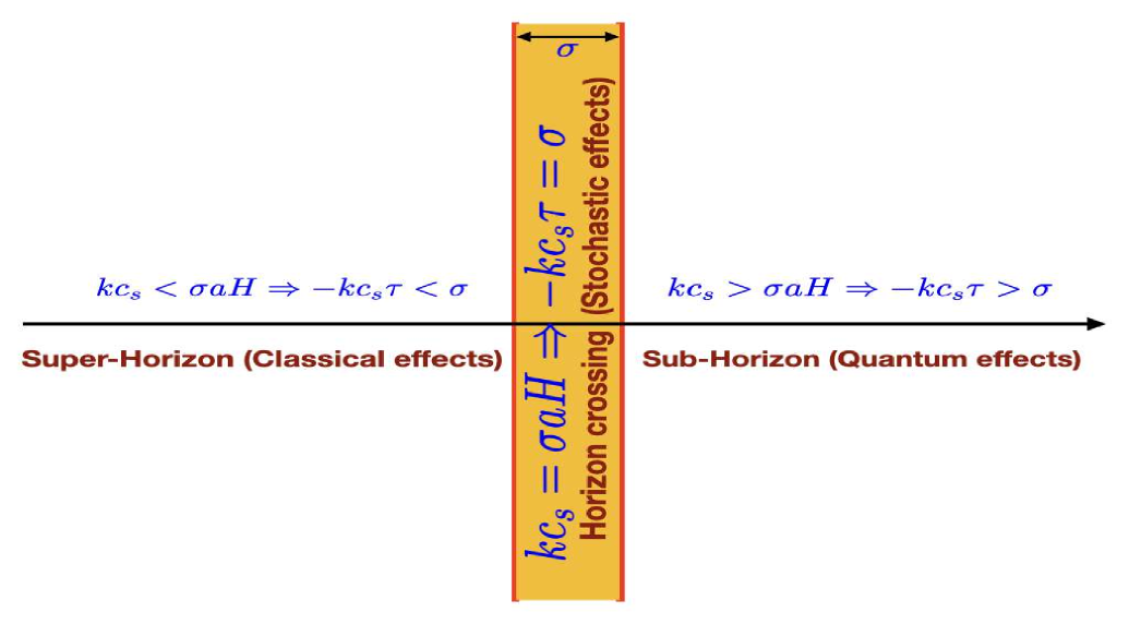
Figure 1: Schematic diagram of stochastic effects taking place for a mode during Horizon crossing. The Horizon is now represented using a region of finite width $\sigma$ where the modes classicalize and become part of the infrared regime after Horizon crossing. As $\sigma$ increases close to $1$ the stochastic effects decrease quickly and so does the width of the orange band. Conversely, for $\sigma\ll 1$, the stochastic effects also increase and similarly the width of orange band increases.

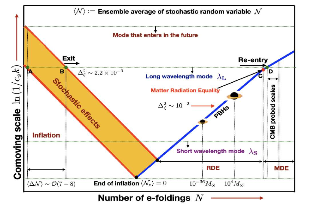
Figure 2: Schematic diagram featuring modes which travel during inflation from the Sub-Horizon, encounter stochastic effects at the Horizon crossing, and later re-enter the Horizon. The long wavelength $\lambda_{L}$ modes associated with the CMB scales exit at the position marked $A$ and $B$ and later re-enter at the instant marked as $D$. The radiation-matter equality is labelled as $C$ which is very close to the CMB re-entry scale. The short wavelength $\lambda_{s}$ are associated with the small length scales near the end of inflation which are responsible for later collapse into PBHs in the radiation-dominated era (RDE) of varied masses. the number of e-folds elapsed between an initial and final set of conditions acts as a stochastic variable ${\cal N}$.

Stochastic inflation is an effective theory approach to studying the long-wavelength components of the inflationary quantum fluctuations. It involves coarse-graining these fluctuations over a fixed scale, just larger than the Hubble radius during the period of inflation. The fixed scale in the Fourier space reads as:

$$k_{\sigma}c_{s}=\sigma aH,$$ (21)

where the stochastic parameter satisfies $\sigma\ll 1$, and this scale behaves as a cut-off for the modes $k$, $-kc_{s}\tau\ll\sigma$ (with $\sigma\ll 1$), that contribute to the coarse-grained sector of the quantum fluctuations. As inflation proceeds, the fluctuations from the small-wavelength or UV (ultraviolet) sector exit the Hubble radius and joins the long-wavelength or infrared (IR) sector increasing its size. The dynamics of the resulting coarse-grained sector of the quantum field is described under the classical stochastic theory by the Langevin equation. Its a stochastic differential equation that includes a classical drift term and the effects from the quantum noise which after horizon exit become part of the classical noise term. The fig. (1) describes the different regimes in the stochastic inflation picture. The quantum effects are most dominant for modes with wavenumber greater than the cut-off scale while the classical effects are understood for the modes with wavenumber smaller than the cut-off. The Horizon crossing boundary becomes an ill-defined concept due to stochastic effects continuously at play.

We refer to the work [164, 43] for discussions on the Hamiltonian formulation in stochastic inflation. To develop the Langevin equations from the Hamilton’s equations, we would first need to identify the UV and IR sectors of the quantum field driving inflation. In order to obtain the Langevin equations in the EFT setup where our variable of interest remains the comoving curvature perturbation $\zeta(t,{\bf x})$, we begin with a similar approach as detailed in [164, 43]. Our starting point would be the second-order perturbed action as mentioned in eqn. (20) for $\zeta(t,{\bf x})$, from which one can calculate the conjugate momentum variable as:

$$\tilde{\Pi}_{\zeta}=\frac{\partial{\cal L}_{\zeta}^{(2)}}{\partial\zeta^{\prime}}=\frac{2M_{p}^{2}a^{2}\epsilon}{c_{s}^{2}}\zeta^{\prime},$$ (22)

using which the corresponding Hamiltonian density after a Legendre transformation can be evaluated as follows,

$${\cal H}_{\zeta}^{(2)} = \tilde{\Pi}_{\zeta}\zeta^{\prime}-{\cal L}^{(2)}_{\zeta}=M_{p}^{2}\int d^{3}x\;a^{2}\Big{(}\frac{\epsilon}{c_{s}^{2}}\Big{)}\Bigg{[}\frac{c_{s}^{4}}{4M_{p}^{4}a^{4}\epsilon^{2}}\tilde{\Pi}^{2}_{\zeta}+c_{s}^{2}(\partial_{i}\zeta)^{2}\Bigg{]}.$$ (23)

Now we can analyze the following Hamilton’s equations of motion using this Hamiltonian density:

$$-\tilde{\Pi}_{\zeta}^{\prime} = \frac{\partial{\cal H}_{\zeta}^{(2)}}{\partial\zeta}=0,$$ (24)

$$\zeta^{\prime} = \frac{\partial{\cal H}_{\zeta}^{(2)}}{\partial\tilde{\Pi}_{\zeta}}=\frac{c_{s}^{2}}{2M_{p}^{2}a^{2}\epsilon}\tilde{\Pi}_{\zeta},$$ (25)

where the prime denotes derivative with respect to the conformal time and the variable $\zeta$ turns out as a cyclic co-ordinate from the Lagrangian ${\cal L}^{(2)}_{\zeta}$. We make change in our choice of time variable from the conformal time to the e-folds $N$ and this leads to the eqn. (25) have the following form:

$$\frac{d\zeta}{dN} = \frac{c_{s}^{2}}{2M_{p}^{2}Ha^{3}\epsilon}\tilde{\Pi}_{\zeta}=\Pi_{\zeta},$$ (26)

$$\frac{d\Pi_{\zeta}}{dN} = \frac{1}{2M_{p}^{2}}\frac{d}{dN}\Bigg{[}\frac{c_{s}^{2}}{Ha^{3}\epsilon}\tilde{\Pi}_{\zeta}\Bigg{]}=\frac{c_{s}^{2}}{2M_{p}^{2}Ha^{3}\epsilon}\tilde{\Pi}_{\zeta}\Bigg{[}2s+\epsilon-3-\eta\Bigg{]}=-(3-\epsilon)\Bigg{[}1-\frac{2(s-\frac{\eta}{2})}{(3-\epsilon)}\Bigg{]}\Pi_{\zeta},$$ (27)

here conversion between the two time variables, $dN/d\tau=Ha$, is used and in the last equality of eqn. (26) we rename the conjugate momentum and remove the tilde. To obtain the other eqn. (27), we perform the derivative of the conjugate momentum with the e-folds $N$ where the third and last lines use the eqn. (24) and definition of $\Pi_{\zeta}$, respectively, and the following definitions for the slow-roll parameters:

$$s=\frac{d\ln c_{s}}{dN},\quad\quad\epsilon=-\frac{d\ln{H}}{dN},\quad\quad\eta=\epsilon-\frac{1}{2}\frac{d\ln{\epsilon}}{dN}.$$ (28)

The above two equations, (26) and (27), will further enable us to determine the Langevin equation governing the dynamics of the coarse-grained supper-Hubble fields in the presence of white noises. The fig. 2 describes the evolution history of the short and long-wavelength modes starting inside the Horizon at very early times, experiencing stochastic effects up to the instant they become classicalized and continue journey in the super-Hubble scales. Different wavelength modes re-enter at different instances in e-foldings. The short-wavelength modes can contribute to the primordial black hole formation while the long-wavelength modes contribute to the CMB observations. The value of the stochastic parameter $\sigma$ characterizes the orange-coloured region describing the stochastic effects. With increasing $\sigma\sim 1$, the stochastic or coarse-graining effects tend to decrease quickly and the band shortens, while, on keeping $\sigma\ll 1$, the band increases in size and similarly points to increase in the duration of stochastic effects.

We start with the quantum operator picture and later present the equations in their classical version on the super-Hubble scales. Now, to obtain the Langevin equations in terms of the curvature perturbations for the coarse-grained components of the initial quantum fields, a decomposition of the said perturbations into its UV and IR components proves beneficial and can be done in the manner:

$$\hat{\Gamma}=\hat{\Gamma}_{\bf IR}+\hat{\Gamma}_{\bf UV}\quad\quad{\rm where}\quad\hat{\Gamma}_{\bf IR}=\{\hat{\zeta},\hat{\Pi}_{\zeta}\}\quad{\rm and}\quad\hat{\Gamma}_{\bf UV}=\{\hat{\zeta}_{s},\hat{\Pi}_{\zeta_{s}}\},$$ (29)

where the subscript $s$ denotes small-wavelength components. These UV components can be expanded in the Fourier modes and get selected upon satisfying $k>k_{\sigma}$ or smaller than the cut-off scale:

$$\hat{\zeta_{s}} = \int_{\mathbb{R^{3}}}\frac{d^{3}k}{(2\pi)^{3}}W\Bigg{(}\frac{k}{k_{\sigma}}\Bigg{)}\Bigg{[}\hat{a}_{{\bf k}}\zeta_{k}(\tau)e^{-i{\bf k}.{\bf x}}+\hat{a}_{{\bf k}}^{\dagger}\zeta_{k}^{*}(\tau)e^{i{\bf k}.{\bf x}}\Bigg{]},$$ (30)

$$\hat{\Pi}_{\zeta_{s}} = \int_{\mathbb{R^{3}}}\frac{d^{3}k}{(2\pi)^{3}}W\Bigg{(}\frac{k}{k_{\sigma}}\Bigg{)}\Bigg{[}\hat{a}_{{\bf k}}\Pi_{\zeta_{k}}(\tau)e^{-i{\bf k}.{\bf x}}+\hat{a}_{{\bf k}}^{\dagger}\Pi_{\zeta_{k}}^{*}(\tau)e^{i{\bf k}.{\bf x}}\Bigg{]}.$$ (31)

These contain the annihilation and creation operators $a_{k}$ and $a_{k}^{\dagger}$ that satisfy the usual canonical commutation relations:

$$[\hat{a_{\bf k}},\hat{a_{\bf k^{\prime}}}^{\dagger}]=\delta^{3}({\bf k}-{\bf k^{\prime}}),\quad\quad[\hat{a_{\bf k}},\hat{a_{\bf k^{\prime}}}]=[\hat{a_{\bf k}^{\dagger}},\hat{a_{\bf k^{\prime}}^{\dagger}}]=0.$$ (32)

The window function $W$ here operates such that:

$$W=\begin{cases}1&k>k_{\sigma}\\ 0&k<k_{\sigma},\end{cases}\\$$ (33)

thereby selecting modes contributing to the small-wavelength or UV sector. Following [164, 43], the Langevin equations from the Hamilton’s equation can be realised using the above mentioned field decomposition and the equations for the UV modes which later play role in the noise terms.

$$\frac{d\hat{\zeta}}{dN} = \hat{\Pi}_{\zeta}+\hat{\xi}_{\zeta}(N),$$ (34)

$$\frac{d\hat{\Pi}_{\zeta}}{dN} = -(3-\epsilon)\hat{\Pi}_{\zeta}\Bigg{[}1-\frac{2(s-\frac{\eta}{2})}{(3-\epsilon)}\Bigg{]}+\hat{\xi}_{\pi_{\zeta}}(N),$$ (35)

The quantities $\hat{\xi}_{\zeta}(N)$ and $\hat{\xi}_{\pi_{\zeta}}(N)$ denote the quantum white noise terms, sourced by the constant outflow of UV modes into the IR modes, and these are further given by:

$$\hat{\xi}_{\zeta} = -\int_{\mathbb{R^{3}}}\frac{d^{3}k}{(2\pi)^{3}}\frac{d}{dN}W\Bigg{(}\frac{k}{k_{\sigma}}\Bigg{)}\Bigg{[}\hat{a}_{{\bf k}}\zeta_{k}(\tau)e^{-i{\bf k}.{\bf x}}+\hat{a}_{{\bf k}}^{\dagger}\zeta_{k}^{*}(\tau)e^{i{\bf k}.{\bf x}}\Bigg{]},$$ (36)

$$\hat{\xi}_{\pi_{\zeta}} = -\int_{\mathbb{R^{3}}}\frac{d^{3}k}{(2\pi)^{3}}\frac{d}{dN}W\Bigg{(}\frac{k}{k_{\sigma}}\Bigg{)}\Bigg{[}\hat{a}_{{\bf k}}\Pi_{\zeta_{k}}(\tau)e^{-i{\bf k}.{\bf x}}+\hat{a}_{{\bf k}}^{\dagger}\Pi_{\zeta_{k}}^{*}(\tau)e^{i{\bf k}.{\bf x}}\Bigg{]},$$ (37)

and the form of the window function $W$ is for convenience chosen to be a Heaviside function:

$$W\Bigg{(}\frac{k}{k_{\sigma}}\Bigg{)}=\Theta\Bigg{(}\frac{k}{k_{\sigma}}-1\Bigg{)}=\Theta\Bigg{(}\frac{k}{\sigma aH}-1\Bigg{)},$$ (38)

where $k_{\sigma}=\sigma aH$. Here $\sigma$ physically represents the stochastic course graining parameter. Next, we compute the expression for the derivative of the window function with respect to the number of e-foldings which is going to be extremely useful to determine the quantized version of the white noise as explicitly mentioned above. Here we have:

$$\frac{d}{dN}W\Bigg{(}\frac{k}{k_{\sigma}}\Bigg{)}=\frac{k}{k_{\sigma}}\left(\epsilon-1\right)\frac{d}{d\tau}W\Bigg{(}\frac{k}{k_{\sigma}}\Bigg{)}=\frac{k}{k_{\sigma}}\left(\epsilon-1\right)k_{\sigma}\delta(k-k_{\sigma})=k\left(\epsilon-1\right)\delta(k-k_{\sigma}).$$ (39)

This function imposes a sharp cut off between IR and UV modes and its derivative with e-folds produces a Dirac Delta distribution $\delta(k-k_{\sigma}(N))$ giving us contributions to the noises after integrating over the various cut-off scales $k_{\sigma}$. Since the noise terms are stochastic in nature this leads to a probabilistic description of the system, which can be analysed in terms of the Langevin Equations. The equations can be solved analytically by a transition into the corresponding Fokker-Planck equation, a second-order partial differential equation, whose construction we review in the next section.

III.2 Fokker-Planck equation from the Langevin equation

This section focuses on briefly discussing the derivation of the Fokker-Planck equation from the Langevin equation. The Fokker-Planck is useful to describe the evolution of the probability distribution of the field variables in the phase space as they evolve during inflation from an initial condition at some arbitrary moment in time to a final field configuration at some another moment later, usually chosen where inflation ends.

To initiate we require the use of a probability rate for the system to start from a given initial field configuration and land to some infinitesimal increment away into a different field configuration in a small increment in the time parameter. To this effect, we introduce the transition probability rate $W_{\Delta{\bf\Gamma}}({\bf\Gamma},N)$ in terms of the field variables, ${\bf\Gamma}=\{\zeta,\Pi_{\zeta}\}$, by the expression:

$$W_{\Delta{\bf\Gamma}}({\bf\Gamma},N)\delta N=P({\bf\Gamma}+\Delta{\bf\Gamma},N+\delta N|{\bf\Gamma},N),$$ (40)

which corresponds to the probability where the system with ${\bf\Gamma}$ at time $N$ evolves to ${\bf\Gamma}+\Delta{\bf\Gamma}$ at $N+\delta N$ in a $\delta N$ infinitesimal increment in time. Using this, equation for the probability $P({\bf\Gamma},N)$ to arrive at a field configuration ${\bf\Gamma}$ starting from some initial configuration ${\bf\Gamma}_{\rm in}$ is given by:

$$\frac{\partial}{\partial N}P({\bf\Gamma},N)=\int d\Delta{\bf\Gamma}\Bigg{[}W_{\Delta{\bf\Gamma}}({\bf\Gamma}-\Delta{\bf\Gamma},N)P({\bf\Gamma}-\Delta{\bf\Gamma},N)-W_{-\Delta{\bf\Gamma}}({\bf\Gamma},N)P({\bf\Gamma},N)\Bigg{]}.$$ (41)

This captures the increase by the first term in going from ${\bf\Gamma}-\Delta{\bf\Gamma}$ to ${\bf\Gamma}$, and the decrease from the second term as we go from ${\bf\Gamma}$ to ${\bf\Gamma}-\Delta{\bf\Gamma}$, and later integrated over the increments $\Delta{\bf\Gamma}$. If we Taylor expand the first term in the integrand of eqn. (41), we notice:

$$W_{\Delta{\bf\Gamma}}({\bf\Gamma}-\Delta{\bf\Gamma},N)P({\bf\Gamma}-\Delta{\bf\Gamma},N)=W_{\Delta{\bf\Gamma}}({\bf\Gamma},N)P({\bf\Gamma},N)+\Bigg{(}-\Delta\Gamma_{i}\frac{\partial}{\partial\Gamma_{i}}+\frac{1}{2}\Delta\Gamma_{i}\Delta\Gamma_{j}\frac{\partial^{2}}{\partial\Gamma_{i}\partial\Gamma_{j}}$$

$$+........+\frac{(-1)^{l}}{l!}\Delta\Gamma_{i}\Delta\Gamma_{j}......\Delta\Gamma_{l}\frac{\partial^{l}}{\partial\Gamma_{i}\partial\Gamma_{j}...\partial\Gamma_{l}}+.....\Bigg{)}[W_{\Delta{\bf\Gamma}}({\bf\Gamma},N)P({\bf\Gamma},N)].$$ (42)

and the dummy indices between the field variables, $\Gamma_{i}=\{\zeta_{i},\Pi_{\zeta,i}\}$, are summed over. The integration variable of the second term in eqn. (41) can be redefined by $\Delta{\bf\Gamma}\rightarrow-\Delta{\bf\Gamma}$ and this enables the following expression:

$$\frac{\partial}{\partial N}P({\bf\Gamma},N)=\sum_{l=1}^{\infty}\frac{(-1)^{l}}{l!}\frac{\partial^{l}}{\partial\Gamma_{i}\partial\Gamma_{j}...\partial\Gamma_{l}}[a_{ij....l}({\bf\Gamma},N)P({\bf\Gamma},N)],$$ (43)

where the various field moments of ${\bf\Gamma}$ are labelled using:

$$a_{ij....l}({\bf\Gamma},N)=\int d\Delta{\bf\Gamma}\;\Delta\Gamma_{i}\Delta\Gamma_{j}....\Delta\Gamma_{l}W_{\Delta{\bf\Gamma}}({\bf\Gamma},N).$$ (44)

these moments will later prove essential to determine the Fokker-Planck differential equation. To evaluate these moments corresponding to the field increments we take help of the Langevin equation, see eqn. (34). Evolving $\bf{\Gamma}$ value between $N$ and $N+\delta N$ where ${\bf\Gamma}=\{\zeta,\Pi_{\zeta}\}$

$${\bf\Gamma}(N+\delta N)={\bf\Gamma}(N)+F({\bf\Gamma})\delta N+G({\bf\Gamma}).\int_{N}^{N+\delta N}\xi(\tilde{N})d\tilde{N}.$$ (45)

where $F({\bf\Gamma})$ encapsulates the classical part of the motion and $G({\bf\Gamma})$ refers to the part which upon squaring forms the noise matrix element arising from the different possible noise correlators,

$$\Sigma_{f_{1},g_{1}}\equiv(G^{2})_{f,g}\delta(\tau_{1}-\tau_{2}),\quad\quad\quad{\rm where},\quad\quad\quad(G^{2})_{f,g}\equiv\Sigma_{f,g}(\tau_{1}),$$ (46)

and the function $\delta(\tau_{1}-\tau_{2})$ represents white noise condition. Further critical details on these matrix elements are expanded in the later section VI. For the current derivation purposes, we now introduce a new notation in terms of a parameter $\alpha$

$${\bf\Gamma}_{\alpha}(N)=(1-\alpha){\bf\Gamma}(N)+\alpha{\bf\Gamma}(N+\delta N),$$ (47)

which allows to parameterize or give certain weights, here $(1-\alpha)$ and $\alpha$, to the position of interest on where to evaluate the functions $F({\bf\Gamma})$ and $G({\bf\Gamma})$. The parameter $\alpha$ can range in between $\alpha\in[0,1]$. In terms of this definition the eqn.(45) becomes:

$${\bf\Gamma}(N+\delta N)={\bf\Gamma}(N)+F({\bf\Gamma}_{\alpha}(N))\delta N+G({\bf\Gamma}_{\alpha}(N)).\int_{N}^{N+\delta N}\xi(\tilde{N})d\tilde{N},$$ (48)

The use of new notation makes it clear that we can solve eqn.(48) in terms of ${\bf\Gamma}(N)$ for any arbitrary $\alpha$. We invoke a perturbative approach to solve by writing

$$\delta{\bf\Gamma}={\bf\Gamma}(N+\delta N)-{\bf\Gamma}(N),$$ (49)

and Taylor expanding functions $F$ and $G$. With the phase space variable in the form

$${\bf\Gamma}_{\alpha}={\bf\Gamma}+\alpha\delta{\bf\Gamma},$$ (50)

we can write eqn.$(\ref{meanGamma})$ as:

$$F_{m}[{\bf\Gamma}_{\alpha}(N)]=F_{m}({\bf\Gamma})+\alpha\delta\Gamma_{i}\frac{\partial}{\partial\Gamma_{i}}F_{m}({\bf\Gamma})+\frac{\alpha^{2}}{2}\delta\Gamma_{i}\delta\Gamma_{j}\frac{\partial^{2}}{\partial\Gamma_{i}\partial\Gamma_{j}}F_{m}({\bf\Gamma})+.....$$ (51)

where the subscript $m$ will be clear shortly in the next equation. Also, a similar analysis can be done for $G[{\Gamma_{\alpha}}(N)]$. By putting these expansions for $F$ and $G$ into eqn. (48), one gets a series in powers of $\delta N$ for the $m$th component of $\delta{\bf\Gamma}$ which has to form:

$$\delta\Gamma_{m}=F_{m}({\bf\Gamma})\delta N+G_{mi}({\bf\Gamma})\int_{N}^{N+\delta N}\xi_{i}(\tilde{N})d\tilde{N}+\alpha G_{pq}({\bf\Gamma})\frac{\partial G_{mj}({\bf\Gamma})}{\partial\Gamma_{p}}\int_{N}^{N+\delta N}\xi_{q}(\tilde{N})d\tilde{N}\int_{N}^{N+\delta N}\xi_{j}(\tilde{N})d\tilde{N}+\cdots,$$ (52)

where the ellipses ‘$\cdots$’ refer to the terms higher-order in the expansion. Using this expression with the eqn.(44) we can finally begin evaluating the moments of field displacement in the following form:

$$a_{i}({\bf\Gamma})=\lim_{\delta N\rightarrow 0}\frac{\langle\delta\Gamma_{i}\rangle}{\delta N}=\Bigg{(}F_{i}({\bf\Gamma})+\alpha G_{mj}({\bf\Gamma})\frac{\partial G_{ij}({\bf\Gamma})}{\partial\Gamma_{m}}\Bigg{)}$$ (53)

$$a_{ij}({\bf\Gamma})=\lim_{\delta N\rightarrow 0}\frac{\langle\delta\Gamma_{i}\delta\Gamma_{j}\rangle}{\delta N}=\Bigg{(}G_{im}({\bf\Gamma})G_{jm}({\bf\Gamma})\Bigg{)},$$ (54)

$$a_{ij.....l}({\bf\Gamma})=0.$$ (55)

where the white noise condition,

$$\langle\xi_{i}(N)\xi_{j}(\tilde{N})\rangle=\delta_{ij}\delta(N-\tilde{N}),$$ (56)

is applied. It becomes clear from the above that only the first and second moments are non-vanishing and putting these into the evolution for the PDF, eqn. (43), we obtain the desired Fokker-Planck equation.

The Fokker-Planck Equation corresponding to the Langevin Equation in terms of the variables ${\bf\Gamma}=\{\zeta,\Pi_{\zeta}\}$ is finally written as:

$$\frac{\partial P({\bf\Gamma},N)}{\partial N}=\mathcal{L}_{\rm FP}({\bf\Gamma})P({\bf\Gamma},N),$$ (57)

where, $\mathcal{L}_{\rm FP}({\bf\Gamma})$ is the Fokker-Planck operator for the probability density function $P({\bf\Gamma},N)$. As a result of the non-zero moments, this Fokker-Planck operator has the form:

$$\mathcal{L}_{\rm FP}({\bf\Gamma})=\Bigg{\{}-\Bigg{(}F_{i}({\bf\Gamma})+\alpha G_{lj}({\bf\Gamma})\frac{\partial G_{ij}({\bf\Gamma})}{\partial\Gamma_{l}}\Bigg{)}\frac{\partial}{\partial\Gamma_{i}}+\frac{1}{2}G_{il}({\bf\Gamma})G_{jl}({\bf\Gamma})\frac{\partial^{2}}{\partial\Gamma_{i}\partial\Gamma_{j}}\Bigg{\}},$$ (58)

Similarly useful is the adjoint Fokker-Planck equation, which has the following differential equation:

$$\frac{\partial}{\partial N}P_{{\bf\Gamma}}(N)=-\mathcal{L}^{\dagger}_{\rm FP}({\bf\Gamma})P_{{\bf\Gamma}}(N).$$ (59)

The corresponding adjoint Fokker-Planck operator is defined when integrating by parts the following operation using the Fokker-Planck operator:

$$\int d{\bf\Gamma}f_{1}({\bf\Gamma})\Bigg{[}\mathcal{L}_{\rm{FP}}({\bf\Gamma}).f_{2}({\bf\Gamma})\Bigg{]}=\int d{\bf\Gamma}\Bigg{[}\mathcal{L}_{\rm FP}^{\dagger}.f_{1}({\bf\Gamma})\Bigg{]}f_{2}({\bf\Gamma}).$$ (60)

There are two important descriptions for interpreting and handling stochastic differential equations :

• Itô prescription $(\alpha=0)$:

  $$\mathcal{L}^{\dagger,\text{It\^{o}}}_{\rm FP}({\bf\Gamma})=\Bigg{\{}F_{i}(\Gamma)\frac{\partial}{\partial\Gamma_{i}}+\frac{1}{2}G_{il}(\Gamma)G_{jl}(\Gamma)\frac{\partial^{2}}{\partial\Gamma_{i}\partial\Gamma_{j}}\Bigg{\}},$$ (61)

• Stratonovich prescription $(\alpha=\frac{1}{2})$ :

  $$\mathcal{L}^{\dagger,\rm{Stratonovich}}_{\rm{FP}}({\bf\Gamma})=\Bigg{\{}F_{i}(\Gamma)\frac{\partial}{\partial\Phi_{i}}+\frac{1}{2}G_{ij}(\Gamma)\frac{\partial G_{lj}(\Gamma)}{\partial\Gamma_{l}}\frac{\partial}{\partial\Gamma_{i}}+\frac{1}{2}G_{il}(\Gamma)G_{jl}(\Gamma)\frac{\partial^{2}}{\partial\Gamma_{i}\partial\Gamma_{j}}\Bigg{\}},$$ (62)

Taking $G=0$ i.e. in the absence of stochastic noise the $\alpha$ term has no significance since differential equations which are deterministic are independent of any prescription. However, the prescription parameter $\alpha$ can become relevant with scenarios where multiple inflating fields on curved field spaces are present. For the purpose of this paper, we are choosing to work in Itô’s prescription, $(\alpha=0)$. The adjoint Fokker-Planck operator can then be written as,

$$\mathcal{L}^{\dagger,\text{It\^{o}}}_{\rm FP}({\bf\Gamma})=\Bigg{(}F_{i}\frac{\partial}{\partial\Gamma_{i}}+\frac{1}{2}\Sigma_{ij}\frac{\partial^{2}}{\partial\Gamma_{i}\partial\Gamma_{j}}\Bigg{)}$$ (63)

where ${\bf\Gamma}=\{\zeta,\Pi_{\zeta}\}$ is the same as before and $F_{i}$ represent the classical drift terms,

$$F_{i}=\Bigg{\{}\Pi_{\zeta},-(3-\epsilon)\Pi_{\zeta}\Bigg{[}1-\frac{2(s-\frac{\eta}{2})}{(3-\epsilon)}\Bigg{]}\Bigg{\}},$$ (64)

where $\Sigma_{ij}$ are the noise correlation matrix elements which we will explicitly determine for our underlying theoretical setup in the later half of this paper.

IV Realising ultra slow-roll phase within the framework of EFT of Stochastic Single Field Inflation

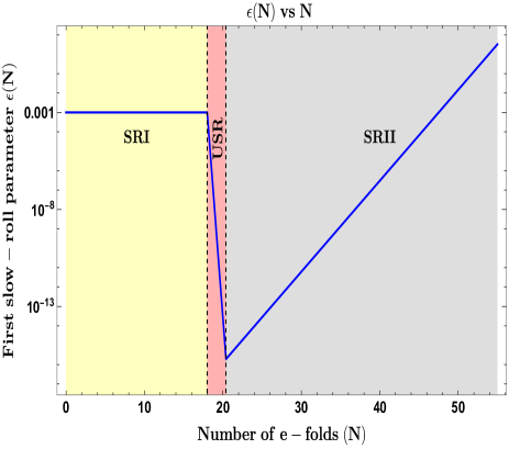
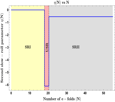
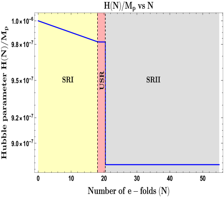
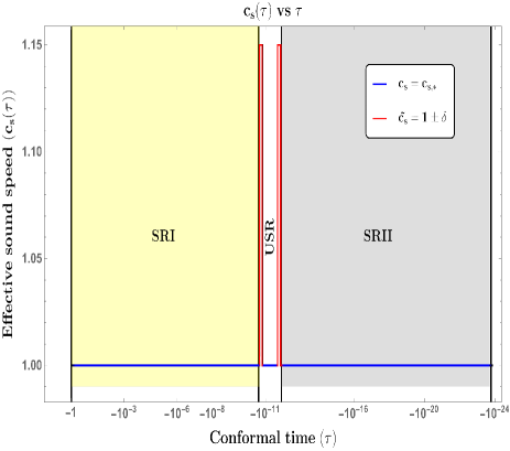
Figure 3: Realisation of the slow-roll and Hubble parameters in the presence of a USR phase during inflation as a function of the e-foldings $N$. The top-left panel shows the $\epsilon(N)$ parameter changing through each phase of the setup, top-right panel for the $\eta(N)$ parameter changing across the same phases, and the bottom-left panel for the Hubble parameter $H(N)$ through each of the respective phases. The bottom-right panel presents a schematic for the effective sound speed $c_{s}$ across the three phases.

In this section we investigate the realisation of the ultra slow-roll phase sandwiched between the slow-roll, SRI and SRII phases, for a stochastic single field inflation framework. We follow the approach of beginning with an particular paramterization of the second slow-roll parameter $\eta$ across the three phases of interest and through that derive the behaviour of the other two parameters, namely $\epsilon$ and the Hubble expansion $H$. This will give us some insights into how a USR phase can be visualised from its effects on the parameters which characterize and are involved in the observables coming from inflation.

The formulas for the slow-roll parameters with respect to the conformal time are defined previously in eqn. (28). Assuming constant $\eta$, the definition for $\epsilon$ gives us:

$$\eta=\epsilon-\frac{1}{2}\frac{d\ln{\epsilon}}{dN}\implies\int_{\epsilon_{i}}^{\epsilon}\frac{d\epsilon}{2\epsilon(\epsilon-\eta)}=\int_{N_{i}}^{N}dN,$$ (65)

which after integration using some initial condition values, $(\epsilon_{i},N_{i})$, leads to the following expression:

$$\epsilon(N)=\eta\bigg{(}1-\bigg{(}1-\frac{\eta}{\epsilon_{i}}\bigg{)}e^{2\eta\Delta N}\bigg{)}^{-1}\sim\left\{\begin{array}[]{ll}\displaystyle\epsilon(N)&\mbox{when}\quad N_{*}\leqslant N\leqslant N_{s}\;(\rm SRI),\\ \displaystyle\displaystyle\epsilon(N_{s})e^{-2\eta(N)(N-N_{s})}&\mbox{when}\quad N_{s}\leqslant N\leqslant N_{e}\;(\rm USR),\\ \displaystyle\displaystyle\epsilon(N_{s})e^{-2\eta(N_{e})(\Delta N_{es})}e^{-2\eta(N)(N-N_{e})}&\mbox{when}\quad N_{e}\leqslant N\leqslant N_{\rm end}\;(\rm SRII),\end{array}\right.$$ (69)

The above equations result from taking appropriate limiting behaviour of the values for the slow-roll parameters in each phase. There complete behaviour is visualised through the fig. (28). The values $\epsilon(N_{s})$ and $\epsilon(N_{s})e^{-2\eta(N_{e})(\Delta N_{es})}$, where $\Delta N_{es}=N_{e}-N_{s}$, acts as the initial condition values for the USR and SRII, respectively, when joining them together. The final $\epsilon$ remains just the sum of its values in the respective regions:

$$\epsilon(N)=\epsilon(N\leqslant N_{s})+\epsilon(N_{s}\leqslant N\leqslant N_{e})+\epsilon(N_{e}\leqslant N\leqslant N_{\rm end}),$$ (70)

In the present work, the $\eta$ parameter remains as a constant value throughout each phase and using the same we can write:

$$\eta(N)=\left\{\begin{array}[]{ll}\displaystyle\eta_{\rm I}(N)&\mbox{when}\quad N_{*}\leqslant N\leqslant N_{s}\;(\rm SRI),\\ \displaystyle\displaystyle\eta_{\rm II}(N)&\mbox{when}\quad N_{s}\leqslant N\leqslant N_{e}\;(\rm USR),\\ \displaystyle\displaystyle\eta_{\rm III}(N)&\mbox{when}\quad N_{e}\leqslant N\leqslant N_{\rm end}\;(\rm SRII),\end{array}\right.$$ (74)

where $\eta_{\rm I},\;\eta_{\rm II},\;\eta_{\rm III}$ are different constants. The above can be expressed using a Heaviside Theta function to join for the three phases as follows:

$$\eta(N)=\eta_{\rm I}(N\leqslant N_{s})+\Theta(N-N_{s})\eta_{\rm II}(N_{s}\leqslant N\leqslant N_{e})+\Theta(N-N_{e})\eta_{\rm III}(N_{e}\leqslant N\leqslant N_{\rm end}),$$ (75)

The Hubble parameter is similarly obtained using the definition of $\epsilon$ as follows:

$$\epsilon(N)=-\frac{d\ln{H}}{dN}\implies H(N)=H_{i}\exp{\bigg{(}-\int_{N_{i}}^{N}\epsilon(N)dN\bigg{)}},$$ (76)

where $H_{i}\equiv H(N_{i})$ is the initial condition value of the Hubble expansion during each phase. For each phase the Hubble can then be expressed as follows:

$$H(N)=\left\{\begin{array}[]{ll}\displaystyle H(N_{*})\exp{\bigg{(}-\int_{N_{*}}^{N}\epsilon(N)dN\bigg{)}}&\mbox{when}\quad N_{*}\leqslant N\leqslant N_{s}\;(\rm SRI),\\ \displaystyle\displaystyle H(N_{s})\exp{\bigg{(}-\int_{N_{s}}^{N}\epsilon(N)dN\bigg{)}}&\mbox{when}\quad N_{s}\leqslant N\leqslant N_{e}\;(\rm USR),\\ \displaystyle\displaystyle H(N_{e})\exp{\bigg{(}-\int_{N_{e}}^{N}\epsilon(N)dN\bigg{)}}&\mbox{when}\quad N_{e}\leqslant N\leqslant N_{\rm end}\;(\rm SRII),\end{array}\right.$$ (80)

and the final expression for the Hubble expansion as function of the e-folds after adding contributions for each phase separately becomes as:

$$H(N)=H(N_{*})\exp{\bigg{(}-\int_{N_{*}}^{N}\epsilon(N)dN\bigg{)}}+H(N_{s})\exp{\bigg{(}-\int_{N_{s}}^{N}\epsilon(N)dN\bigg{)}}+H(N_{e})\exp{\bigg{(}-\int_{N_{e}}^{N}\epsilon(N)dN\bigg{)}},$$ (81)

where $H(N_{*}),\;H(N_{s}),\;H(N_{e})$ comes as initial conditions from the continuity of values between the different phases.

We now follow the plots in fig. 3, 3. Initially in the SRI, which starts from the instant $N_{*}$ and where slow-roll conditions are necessarily met, $\eta$ behaves almost as a negatively small and constant quantity and similarly $\epsilon$ also stays as a small constant quantity. This happens until a deviation from standard slow-roll arguments is encountered after a certain number of e-folds $N_{s}$. This instant marks the transition into the next phase where a significant violation of slow-roll condition can take place. The nature of the transition at $N_{s}$ is chosen for the present work as a sharp transition, modelled by a Heaviside Theta function $\Theta(k-k_{s})$, where $k_{s}$ is the corresponding transition wavenumber. The magnitude of $\eta$ greatly increases in the USR, as we will also see in the later eqn. (103), and in a similar manner $\epsilon$ suffers a drastic decrease in magnitude, see eqn. (102). Such behaviour as mentioned persists till the duration of USR comes to an end at the instant $N_{e}$, with the corresponding wavenumber $k_{e}$. Soon after exiting from the USR, another sharp transition of the form $\Theta(k-k_{e})$ is found to take effect and the slow-roll conditions starts to restore. The parameters $\epsilon$ and $\eta$ in the SRII start to increase throughout the whole phase till they achieve values of magnitude ${\cal O}(1)$ and the associated instant in e-folds $N_{\rm end}$ marks the end of inflation. For successful inflation in the set up one requires for the total change in e-foldings from the initial moment $N_{*}$ to lie within $\Delta N_{\rm Total}=N_{\rm end}-N_{*}\sim{\cal O}(55-60).$

The plot in fig. 3 describes the effective sound speed $c_{s}$ parameterization for the present set up. Here we choose to have $c_{s}(\tau=\tau_{*})=c_{s,*}=1$ in the initial slow-roll phase, where $c_{s,*}$ is the corresponding value at the pivot scale. The condition $c_{s}=1$ refers to a canonical stochastic single-field inflation model. When near the instant of sharp transition, at conformal time $\tau=\tau_{s}$ with $N=N_{s}$, the effective sound speed changes from its previous to a new value labelled here as $\tilde{c_{s}}=1\pm\delta$, where $\delta\ll 1$ is a fine-tuning variable. This sudden jump in its magnitude is what forces the sharp nature of the transition in between the SRI and the USR phase. Again throughout the USR ($\tau_{s}\leqslant\tau\leqslant\tau_{e}$) , the sound speed changes back to $c_{s}$. At the instant of the second sharp transition, $\tau=\tau_{e}$, we once again observe the value to experience sudden change into $c_{s}=\tilde{c_{s}}=1\pm\delta$, after which into the SRII phase the sound speed reverts back to $c_{s}$ till we encounter the end of inflation at the conformal time instant $\tau=\tau_{\rm end}$ or $N=N_{\rm end}$.

The aforementioned parameterization of the effective sound speed can also be written for the three regions, including at instances of the sharp transitions, in the following manner:

$$c_{s}(\tau)=\left\{\begin{array}[]{ll}\displaystyle c_{s,*}&\mbox{when}\quad\tau_{*}\leqslant\tau<\tau_{s}\;(\rm SRI),\\ \displaystyle\displaystyle\tilde{c_{s}}=1\pm\delta&\mbox{when}\quad\tau=\tau_{s}\;(\rm USR),\\ \displaystyle\displaystyle c_{s,*}&\mbox{when}\quad\tau_{s}<\tau<\tau_{e}\;(\rm USR),\\ \displaystyle\displaystyle\tilde{c_{s}}=1\pm\delta&\mbox{when}\quad\tau=\tau_{e}\;(\rm SRII),\\ \displaystyle\displaystyle c_{s,*}&\mbox{when}\quad\tau_{e}<N<\tau_{\rm end}\;(\rm SRII),\end{array}\right.$$ (87)

where $c_{s,*}=c_{s}(\tau=\tau_{*})$ is the value at the instance of pivot scale as mentioned in the above explanation of the parameterization.

V Modes representing comoving scalar curvature perturbation

This section focuses on developing the solutions for the comoving curvature perturbation in a quasi de Sitter background from the underlying EFT in inflation formalism. We employ the decoupling limit to safely examine the behaviour of the mode solutions for the three phases comprising our setup of SR, USR, and SRII. The general formulas once understood will later help to construct the various elements of the scalar power spectrum by finding correlations among the comoving curvature perturbation and its conjugate momentum variable.

In this section we analyse the MS equation solutions for the three distinct phases in our setup during inflation. The solutions obtained will later prove important for our analysis of the Power Spectrum and and to establish the corresponding noise matrix elements. The variation of the action eqn. (20) allows one to obtain the Mukhanov-Sasaki (MS) equation and solving it in the Fourier space provides us with the curvature perturbation modes for different phases. The MS equation in the Fourier space takes on the form,

$$\bigg{(}\partial^{2}_{\tau}+2\frac{z^{\prime}(\tau)}{z(\tau)}\partial_{\tau}+c_{s}^{2}k^{2}\bigg{)}\zeta_{\bf k}(\tau)=0.$$ (88)

Here $z(\tau)$ is known as the Mukhanov-Sasaki variable which is given by the following expression:

$$z(\tau):=\frac{a(\tau)\sqrt{2\epsilon}}{c_{s}}\quad\quad\quad{\rm where}\quad\quad\quad a(\tau)=-\frac{1}{H\tau}\quad\quad\quad{\rm with}-\infty<\tau<0.$$ (89)

Now we use the following results which will be extremely useful to solve the above-mentioned second order differential equation:

$$\frac{z^{\prime}(\tau)}{z(\tau)}={\cal H}\left(1-\eta+\epsilon-s\right)=-\frac{1}{\tau}\left(1-\eta+\epsilon-s\right)\quad\quad\quad{\rm where}\quad\quad\quad s:=\frac{c^{{}^{\prime}}_{s}}{{\cal H}c_{s}},$$ (90)

and

$$\frac{z^{\prime\prime}(\tau)}{z(\tau)}={\cal H}^{2}\left(1-\eta+\epsilon-s\right)^{2}+{\cal H}^{{}^{\prime}}\left(1-\eta+\epsilon-s\right)=2{\cal H}^{2}\left(1-\frac{\eta}{2}+\frac{3}{2}\epsilon-\frac{3}{2}s\right)=\frac{1}{\tau^{2}}\left(\nu^{2}--\frac{1}{4}\right),\quad\quad\quad$$ (91)

where the parameter $\nu$ is defined by the following expression:

$$\nu:=\frac{3}{2}+3\epsilon-\eta-3s.$$ (92)

Here $s$ is another slow-roll parameter in all the three phases and $\nu=3/2$ represents the de Sitter limiting solution in the present context of discussion.

V.1 First Slow Roll phase (SRI)

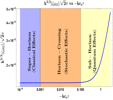
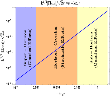
Figure 4: Behaviour of the curvature perturbation and its conjugate momentum mode in the SRI as a function of $-kc_{s}\tau$. The left-panel shows evolution of $k^{3/2}|\zeta_{\rm SRI}|/\sqrt{2}\pi$ after choosing the Bunch-Davies initial conditions $(\alpha_{1}=1,\beta_{1}=0)$ and $\nu\sim 3/2$. Similarly, the right-panel shows evolution of $|k^{1/2}\Pi_{\rm SRI}|/\sqrt{2}\pi$. The orange shaded region represents the stochastic effects where $-kc_{s}\tau=\sigma\in(0.001,0.1)$. The stochastic parameter $\sigma$ acts a coarse-graining factor and explains the quantum-to-classical transition of the modes. The blue and yellow shaded regions highlights the quantum and classical effects, respectively.

The general solution for the MS equation (88) in the first slow-roll or SRI region for a quasi de Sitter background and arbitrary initial quantum vacuum state is as follows,

$${\bf\zeta}_{\bf SRI}=\frac{2^{\nu-\frac{3}{2}}c_{s}H(-kc_{s}\tau)^{\frac{3}{2}-\nu}}{i\sqrt{2\epsilon}(kc_{s})^{\frac{3}{2}}\sqrt{2}M_{p}}\Bigg{|}\frac{\Gamma(\nu)}{\Gamma(\frac{3}{2})}\Bigg{|}\Bigg{\{}\alpha_{1}(1+ikc_{s}\tau)e^{-i(kc_{s}\tau+\frac{\pi}{2}(\nu+\frac{1}{2}))}-\beta_{1}(1-ikc_{s}\tau)e^{i(kc_{s}\tau+\frac{\pi}{2}(\nu+\frac{1}{2}))}\Bigg{\}}.$$ (93)

The mode function for the canonically conjugate momentum can be obtained by differentiating $\zeta_{\rm SRI}$,

$${\bf\Pi_{\zeta}}_{\bf SRI}={\bf\zeta^{\prime}}_{\bf SRI}=\frac{2^{\nu-\frac{3}{2}}c_{s}H(-kc_{s}\tau)^{\frac{3}{2}-\nu}}{i\tau\sqrt{2\epsilon}(kc_{s})^{\frac{3}{2}}\sqrt{2}M_{p}}\Bigg{|}\frac{\Gamma(\nu)}{\Gamma(\frac{3}{2})}\Bigg{|}\Bigg{[}\alpha_{1}\Bigg{\{}\Bigg{(}\frac{3}{2}-\nu\Bigg{)}(1+ikc_{s}\tau)+k^{2}c_{s}^{2}\tau^{2}\Bigg{\}}e^{-i(kc_{s}\tau+\frac{\pi}{2}(\nu+\frac{1}{2}))}$$

$$-\beta_{1}\Bigg{\{}\Bigg{(}\frac{3}{2}-\nu\Bigg{)}(1-ikc_{s}\tau)+k^{2}c_{s}^{2}\tau^{2}\Bigg{\}}e^{i(kc_{s}\tau+\frac{\pi}{2}(\nu+\frac{1}{2}))}\Bigg{]},$$ (94)

where in the above solutions $\alpha_{1}$ and $\beta_{1}$ are the Bogoliubov coefficients in the SRI region which can be fixed using initial conditions in form of choosing a suitable quantum vacuum state. The SRI phase persists for the interval $\tau<\tau_{s}$. At $\tau=\tau_{s}$, the SRI transits to the Ultra Slow Roll (USR) and the nature of this transition will be of utter importance for rest of the analysis. During SRI, $\epsilon$ is approximately a constant quantity that varies very slowly with time scale whereas the second slow roll parameter, $\eta$, is very small and can be treated almost as a constant,

$$\epsilon=-\frac{\dot{H}}{H^{2}}=\Bigg{(}1-\frac{\mathcal{H}^{\prime}}{\mathcal{H}^{2}}\Bigg{)},$$ (95)

$$\eta=\epsilon-\frac{1}{2}\frac{\epsilon^{\prime}}{\epsilon\mathcal{H}}.$$ (96)

If we choose the well-known Euclidean quantum vacuum state i.e. the Bunch-Davies vacuum state, then in the SRI period the corresponding Bogoliubov coefficients are given by the following expression:

$$\alpha_{1}=1,\quad\beta_{1}=0.$$ (97)

After substituting the mentioned values of the Bogoliubov coefficients for SRI the expression for the comoving curvature perturbation in the case of Bunch Davies initial vacuum state can be further recast in the following form:

$${\bf\zeta}_{{\bf SRI},{\bf BD}}=\frac{2^{\nu-\frac{3}{2}}\,c_{s}\,H(-kc_{s}\tau)^{\frac{3}{2}-\nu}}{i\sqrt{2\epsilon}(kc_{s})^{3/2}\sqrt{2}M_{p}}\Bigg{|}\frac{\Gamma(\nu)}{\Gamma(\frac{3}{2})}\Bigg{|}(1+ikc_{s}\tau)e^{-i(kc_{s}\tau+\frac{\pi}{2}(\nu+\frac{1}{2}))}.$$ (98)

Under the similar Bunch-Davies initial conditions, the canonically conjugate momentum has the following form

$${\bf\Pi_{\zeta}}_{{\bf SRI},{\bf BD}}={\bf\zeta^{\prime}}_{{\bf SRI},{\bf BD}}=\frac{2^{\nu-\frac{3}{2}}c_{s}H(-kc_{s}\tau)^{\frac{3}{2}-\nu}}{i\tau\sqrt{2\epsilon}(kc_{s})^{\frac{3}{2}}\sqrt{2}M_{p}}\Bigg{|}\frac{\Gamma(\nu)}{\Gamma(\frac{3}{2})}\Bigg{|}\Bigg{\{}\Bigg{(}\frac{3}{2}-\nu\Bigg{)}(1+ikc_{s}\tau)+k^{2}c_{s}^{2}\tau^{2}\Bigg{\}}e^{-i(kc_{s}\tau+\frac{\pi}{2}(\nu+\frac{1}{2}))}.$$ (99)

On further implementing the limiting case of $\nu=3/2$ in the above derived result one can get the simplified expressions in the case of exact de Sitter space-time. In this limit, the comoving curvature perturbation attains the following simplified form:

$${\bf\zeta}_{{\bf SRI},{\bf dS}}=\frac{ic_{s}H}{\sqrt{2\epsilon}(kc_{s})^{\frac{3}{2}}\sqrt{2}M_{p}}(1+ikc_{s}\tau)e^{-ikc_{s}\tau}.$$ (100)

Similarly, the exact de Sitter solution for the canonically conjugate momentum looks as,

$${\bf\Pi_{\zeta}}_{{\bf SRI},{\bf dS}}={\bf\zeta^{\prime}}_{{\bf SRI},{\bf dS}}=\frac{ic_{s}H}{\tau\sqrt{2\epsilon}(kc_{s})^{\frac{3}{2}}\sqrt{2}M_{p}}\;k^{2}c_{s}^{2}\tau^{2}\;e^{-ikc_{s}\tau}.$$ (101)

The figure fig. 4 describes evolution of scalar curvature perturbation mode and its conjugate momenta as function of the dimensionless variable $-kc_{s}\tau$. The solution used is a result of choosing the Bunch-Davies initial vacuum conditions, $(\alpha_{1}=1,\beta_{1}=0)$ and taking the limiting case of $\nu\sim 3/2$. In 4 we notice from the blue line how the modulus $|\zeta_{\rm SRI}|$ for a given mode behaves when inside the Horizon, after which its amplitude decays upon reaching the boundary where stochastic effects starts to take effect. In the stochastic inflation formalism, there is an additional stochastic parameter $\sigma$ ($\sigma\ll 1$) which acts as a coarse-graining factor and creates a region in the super-Horizon through which short-wavelength modes transit and observe a quantum-to-classical transition until finally get treated as long-wavelength modes in the super-Horizon. In the super-Horizon, where classical effects dominates, the quantity $|\zeta_{\rm SRI}|$ becomes a constant. The conjugate momenta related quantity $|\Pi_{\rm SRI}|$ is shown in 4 where throughout the three regimes in the quantum-to-classical transition, the said quantity observes drastic decrease in its value as the conjugate momenta mode finally becomes super-Horizon where its the most suppressed.

V.2 Ultra Slow Roll phase (USR)

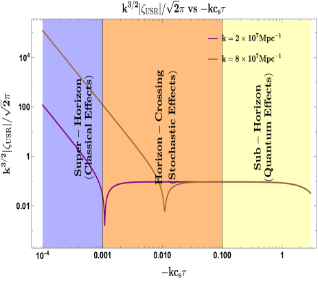
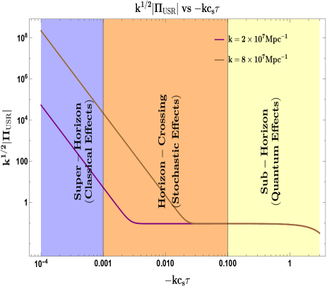
Figure 5: Behaviour of the curvature perturbation and its conjugate momentum mode in the USR as a function of $-kc_{s}\tau$. The left-panel shows evolution of $k^{3/2}|\zeta_{\rm USR}|/\sqrt{2}\pi$ after choosing the Bunch-Davies initial conditions $(\alpha_{2,{\bf dS}},\beta_{2,{\bf dS}})$ and $\nu\sim 3/2$. Similarly, the right-panel shows evolution of $|k^{1/2}\Pi_{\rm USR}|/\sqrt{2}\pi$. The orange shaded region represents the stochastic effects where $-kc_{s}\tau=\sigma\in(0.001,0.1)$. The stochastic parameter $\sigma$ acts as a coarse-graining parameter near Horizon corssing where it the quantum-to-classical transition of the modes take place. The blue and yellow shaded regions highlights the quantum and classical effects, respectively.

The USR phase operates during the conformal time interval $\tau_{s}\leqslant\tau\leqslant\tau_{e}$ where, $\tau_{s}$ is the time when SRI ends and USR begins and $\tau_{e}$ is the time when USR ends and the following SRII begins. The slow-roll parameter $\epsilon$ in the USR now become extremely suppressed and time-dependent which can be described in terms of $\epsilon$ as,

$$\epsilon(\tau)=\epsilon\Bigg{(}\frac{a(\tau_{s})}{a(\tau)}\Bigg{)}^{6}=\epsilon\Bigg{(}\frac{\tau}{\tau_{s}}\Bigg{)}^{6}.$$ (102)

Important is the behaviour of the second slow-roll parameter $\eta(\tau)$ that varies with time in the USR as follows,

$$\eta(\tau)\sim\eta-6\approx{\cal O}(-6).$$ (103)

It is to be noted here that we have considered a sharp transition when going from the SRI to USR. Now, the general solution for the MS equation (88) in the USR region with an arbitrary quantum vacuum state can be expressed using the following simplified form,

$${\bf\zeta}_{\bf USR}=\frac{2^{\nu-\frac{3}{2}}c_{s}H(-kc_{s}\tau)^{\frac{3}{2}-\nu}}{i\sqrt{2\epsilon}(kc_{s})^{\frac{3}{2}}\sqrt{2}M_{p}}\Bigg{[}\frac{\tau_{s}}{\tau}\Bigg{]}^{3}\Bigg{|}\frac{\Gamma(\nu)}{\Gamma(\frac{3}{2})}\Bigg{|}\Bigg{\{}\alpha_{2}(1+ikc_{s}\tau)e^{-i(kc_{s}\tau+\frac{\pi}{2}(\nu+\frac{1}{2}))}-\beta_{2}(1-ikc_{s}\tau)e^{i(kc_{s}\tau+\frac{\pi}{2}(\nu+\frac{1}{2}))}\Bigg{\}}.$$ (104)

Also, the corresponding canonically conjugate momentum mode function can be obtained by differentiating $\zeta_{\bf USR}$,

$${\bf\Pi_{\zeta}}_{\bf USR}={\bf\zeta^{\prime}}_{\bf USR}=\frac{2^{\nu-\frac{3}{2}}c_{s}H(-kc_{s}\tau)^{\frac{3}{2}-\nu}\tau_{s}^{3}}{i\sqrt{2\epsilon}(kc_{s})^{\frac{3}{2}}\sqrt{2}M_{p}\,\tau^{4}}\Bigg{|}\frac{\Gamma(\nu)}{\Gamma(\frac{3}{2})}\Bigg{|}\Bigg{[}\Bigg{\{}k^{2}c_{s}^{2}\tau^{2}+(1+ikc_{s}\tau)\Bigg{(}\Bigg{(}\frac{3}{2}-\nu\Bigg{)}-3\Bigg{)}\Bigg{\}}\alpha_{2}e^{-i(kc_{s}\tau+\frac{\pi}{2}(\nu+\frac{1}{2}))}$$

$$-\Bigg{\{}k^{2}c_{s}^{2}\tau^{2}+(1-ikc_{s}\tau)\Bigg{(}\Bigg{(}\frac{3}{2}-\nu\Bigg{)}-3\Bigg{)}\Bigg{\}}\beta_{2}e^{i(kc_{s}\tau+\frac{\pi}{2}(\nu+\frac{1}{2}))}\Bigg{]},\quad\quad$$ (105)

where, $\alpha_{2}$ and $\beta_{2}$ are the Bogoliubov coefficients in the USR region that can be found in terms of $\alpha_{1}$ and $\beta_{1}$ using the two boundary conditions interpreted as Israel junction conditions at time scale $\tau=\tau_{s}$ .

The first condition implies that the scalar modes obtained are continuous at the sharp transition point, $\tau=\tau_{s}$ between SRI and USR

$$[\zeta(\tau)]_{\bf SRI,\tau=\tau_{s}}=[\zeta(\tau)]_{\bf USR,\tau=\tau_{s}}.$$ (106)

The second condition implies that momentum modes are continuous at the sharp transition point $\tau=\tau_{s}$ between SRI and USR

$$[\zeta^{\prime}(\tau)]_{{\bf SRI},\,{\bf\tau=\tau_{s}}}=[\zeta^{\prime}(\tau)]_{\bf USR,\,\tau=\tau_{s}}.$$ (107)

After applying the above two junction conditions we obtain two constraint equations for Bogoliubov coefficients in the USR region

$$\alpha_{2}=\frac{1}{2k^{3}\tau_{s}^{3}c_{s}^{3}}\Bigg{\{}\Bigg{(}3i+3ik^{2}c_{s}^{2}\tau_{s}^{2}+2k^{3}c_{s}^{3}\tau_{s}^{3}\Bigg{)}\alpha_{1}-\Bigg{(}3i+6kc_{s}\tau_{s}-3ik^{2}c_{s}^{2}\tau_{s}^{2}\Bigg{)}\beta_{1}e^{i\left(2k\tau_{s}c_{s}+\pi\left(\nu+\frac{1}{2}\right)\right)}\Bigg{\}},$$ (108)

$$\beta_{2}=\frac{1}{2k^{3}c_{s}^{3}\tau_{s}^{3}}\Bigg{\{}\Bigg{(}3i-6kc_{s}\tau_{s}-3ik^{2}c_{s}^{2}\tau_{s}^{2}\Bigg{)}\alpha_{1}e^{-i(\pi(\nu+\frac{1}{2})+2kc_{s}\tau_{s})}-\Bigg{(}3i+3ik^{2}c_{s}^{2}\tau_{s}^{2}-2k^{3}c_{s}^{3}\tau_{s}^{3}\Bigg{)}\beta_{1}\Bigg{\}}.$$ (109)

Implementing the Bunch Davies initial vacuum state $(\alpha_{1}=1,\,\beta_{1}=0)$ into the USR Bogoliubov coefficients we get the simplified form of $\alpha_{2}$ and $\beta_{2}$

$$\alpha_{{2},{\bf BD}}=\frac{1}{2k^{3}\tau_{s}^{3}c_{s}^{3}}\Bigg{(}3i+3ik^{2}c_{s}^{2}\tau_{s}^{2}+2k^{3}c_{s}^{3}\tau_{s}^{3}\Bigg{)},$$ (110)

$$\beta_{{2},{\bf BD}}=\frac{1}{2k^{3}c_{s}^{3}\tau_{s}^{3}}\Bigg{(}3i-6kc_{s}\tau_{s}-3ik^{2}c_{s}^{2}\tau_{s}^{2}\Bigg{)}e^{-i(\pi(\nu+\frac{1}{2})+2kc_{s}\tau_{s})}.$$ (111)

Further implementing the limiting case $\nu=\frac{3}{2}$ in Bunch Davies vacuum derived result one can get the simplified expression for USR Bogoliubov coefficients in the case of de Sitter space

$$\alpha_{{2},{\bf dS}}=\frac{1}{2k^{3}\tau_{s}^{3}c_{s}^{3}}\Bigg{(}3i+3ik^{2}c_{s}^{2}\tau_{s}^{2}+2k^{3}c_{s}^{3}\tau_{s}^{3}\Bigg{)},$$ (112)

$$\beta_{{2},{\bf dS}}=\frac{1}{2k^{3}c_{s}^{3}\tau_{s}^{3}}\Bigg{(}3i-6kc_{s}\tau_{s}-3ik^{2}c_{s}^{2}\tau_{s}^{2}\Bigg{)}e^{-2ikc_{s}\tau_{s}}.$$ (113)

The mode function in the limiting case $\nu=\frac{3}{2}$ in Bunch Davies vacuum gives rise to the de Sitter result which can be further written as:

$${\bf\zeta}_{{\bf USR},{\bf dS}}=\frac{ic_{s}H}{\sqrt{2\epsilon}(kc_{s})^{\frac{3}{2}}\sqrt{2}M_{p}}\Bigg{[}\frac{\tau_{s}}{\tau}\Bigg{]}^{3}\Bigg{\{}\alpha_{{2},{\bf dS}}(1+ikc_{s}\tau)e^{-ikc_{s}\tau}-\beta_{{2},{\bf dS}}(1-ikc_{s}\tau)e^{ikc_{s}\tau}\Bigg{\}}.$$ (114)

The momentum mode function for the above case is:

$${\bf\Pi_{\zeta}}_{{\bf USR},{\bf dS}}={\bf\zeta^{\prime}}_{{\bf USR},{\bf dS}}=\frac{ic_{s}H\tau_{s}^{3}}{\sqrt{2\epsilon}(kc_{s})^{\frac{3}{2}}\sqrt{2}M_{p}\,\tau^{4}}\Bigg{[}\Bigg{\{}k^{2}c_{s}^{2}\tau^{2}-3(1+ikc_{s}\tau)\Bigg{\}}\alpha_{{2},{\bf dS}}e^{-ikc_{s}\tau}$$

$$-\Bigg{\{}k^{2}c_{s}^{2}\tau^{2}-3(1-ikc_{s}\tau)\Bigg{\}}\beta_{{2},{\bf dS}}e^{ikc_{s}\tau}\Bigg{]}.$$ (115)

The figure fig. 5 describes evolution in the USR of the scalar curvature perturbation mode and its conjugate momenta as function of the dimensionless variable $-kc_{s}\tau$. Similar to SRI, we continue with our choice of Bunch-Davies initial condition for the Bogoliubov coefficients in this phase and taking the limit $\nu\sim 3/2$, which leads to the coefficients $(\alpha_{2,{\bf dS}},\beta_{2,{\bf dS}})$, see eqn. (112,113). Here we plot the behaviour for different wavenumbers where the additional momentum dependence comes from using the quantity $k_{s}c_{s}\tau_{s}$ in the mode solutions. The plot is shown after choosing $k_{s}c_{s}\tau_{s}\sim{\cal O}(-0.01)$. From 5, we notice that the magnitude $|\zeta_{\rm USR}|$ stays constant when in the sub-Horizon. Near the Horizon crossing, various short-scale modes encounter stochastic effects and they undergo a quantum-to-classical transition until finally in the super-Horizon regime. In this regime, the quantity $|\zeta_{\rm USR}|$ tends to increase greatly, however, when concerned with the behaviour of the modes near the Horizon crossing, including stochastic effects the strength of the modulus is sufficient enough to give $k^{3}|\zeta_{\rm USR}|^{2}\sim{\cal O}(10^{-3}-10^{-2})$. In fig. 5, the evolution of the conjugate momenta mode in the USR is shown. This time the conjugate momenta has a significant role to play, as seen from the magnitude of $|\Pi_{\rm USR}|$. During Horizon crossing, in presence of the stochastic effects, the mode starts to increase in strength and keeps going monotonically as they become of long-wavelength in the super-Horizon scales.

V.3 Second Slow Roll phase (SRII)

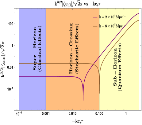
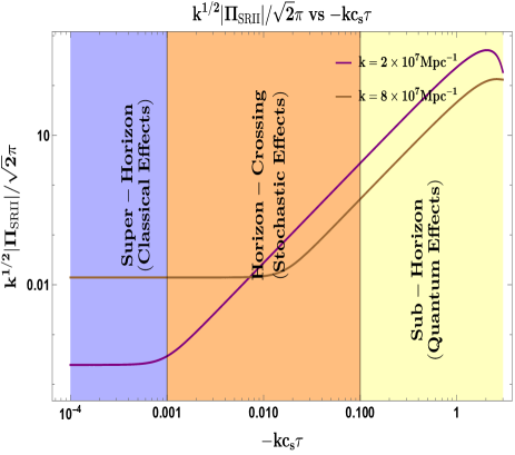
Figure 6: Behaviour of the curvature perturbation and its conjugate momentum mode in the SRII as a function of $-kc_{s}\tau$. The left-panel shows evolution of $k^{3/2}|\zeta_{\rm SRII}|/\sqrt{2}\pi$ after choosing the Bunch-Davies initial conditions $(\alpha_{3,{\bf dS}},\beta_{3,{\bf dS}})$ and $\nu\sim 3/2$. Similarly, the right-panel shows evolution of $|k^{1/2}\Pi_{\rm SRII}|/\sqrt{2}\pi$. The orange shaded region represents the stochastic effects where $-kc_{s}\tau=\sigma\in(0.001,0.1)$. The stochastic parameter $\sigma$ acts as a coarse-graining parameter near Horizon corssing where it the quantum-to-classical transition of the modes take place. The blue and yellow shaded regions highlights the quantum and classical effects, respectively.

The second slow roll phase persists for the conformal time scale $\tau_{e}\leqslant\tau\leqslant\tau_{\rm end}$ where, $\tau_{e}$ marks the end of USR phase and beginning of SRII phase whereas $\tau_{\rm end}$ marks the end of inflationary paradigm. The dependence of first and second slow roll parameters can be described as :

$$\epsilon(\tau)=\epsilon\Bigg{(}\frac{a(\tau_{s})}{a(\tau_{e})}\Bigg{)}^{6}=\epsilon\Bigg{(}\frac{\tau_{e}}{\tau_{s}}\Bigg{)}^{6}\longrightarrow\epsilon(\tau=\tau_{end})=1,$$ (116)

$$\eta(\tau)=\eta\longrightarrow\eta(\tau=\tau_{end})\sim\mathcal{O}(-1).$$ (117)

where, $\epsilon$ is slow roll parameter in SRI region . In the preceding section we have considered sharp transition at the boundary of transition between SRI to USR here also we considered the sharp transition from USR to SRII region. Imposing the two boundary conditions termed as Israel junction condition the constraint relation for Bogoliubov coefficients in the SRII region can be deduced. The mode solution for SRII region is:

$${\bf\zeta}_{\bf SRII}=\frac{2^{\nu-\frac{3}{2}}c_{s}H(-kc_{s}\tau)^{\frac{3}{2}-\nu}}{i\sqrt{2\epsilon}(kc_{s})^{\frac{3}{2}}\sqrt{2}M_{p}}\Bigg{[}\frac{\tau_{s}}{\tau_{e}}\Bigg{]}^{3}\Bigg{|}\frac{\Gamma(\nu)}{\Gamma(\frac{3}{2})}\Bigg{|}\Bigg{\{}\alpha_{3}(1+ikc_{s}\tau)e^{-i\left(kc_{s}\tau+\frac{\pi}{2}(\nu+\frac{1}{2})\right)}-\beta_{3}(1-ikc_{s}\tau)e^{i\left(kc_{s}\tau+\frac{\pi}{2}(\nu+\frac{1}{2})\right)}\Bigg{\}}.$$ (118)

The canonically conjugate momentum mode function can be obtained by differentiating $\zeta_{\bf SRII}$ and is expressed as:

$${\bf\Pi_{\zeta}}_{\bf SRII}={\bf\zeta^{\prime}}_{\bf SRII}=\frac{2^{\nu-\frac{3}{2}}c_{s}H(-kc_{s}\tau)^{\frac{3}{2}-\nu}}{i\sqrt{2\epsilon}(kc_{s})^{\frac{3}{2}}\sqrt{2}M_{p}\,\tau}\Bigg{[}\frac{\tau_{s}}{\tau_{e}}\Bigg{]}^{3}\Bigg{|}\frac{\Gamma(\nu)}{\Gamma(\frac{3}{2})}\Bigg{|}\Bigg{\{}\alpha_{3}\Bigg{\{}k^{2}c_{s}^{2}\tau^{2}+(1+ikc_{s}\tau)\Bigg{(}\frac{3}{2}-\nu\Bigg{)}\Bigg{\}}e^{-i\left(kc_{s}\tau+\frac{\pi}{2}(\nu+\frac{1}{2})\right)}$$

$$-\beta_{3}\Bigg{\{}k^{2}c_{s}^{2}\tau^{2}+(1-ikc_{s}\tau)\Bigg{(}\frac{3}{2}-\nu\Bigg{)}\Bigg{\}}e^{i\left(kc_{s}\tau+\frac{\pi}{2}(\nu+\frac{1}{2})\right)}\Bigg{\}},$$ (119)

where, $\alpha_{3}$ and $\beta_{3}$ are the Bogoliubov coefficients. The constraint relation for these coefficients can be found in terms of $\alpha_{2}$ and $\beta_{2}$ using the boundary conditions termed as Israel junction conditions. The underlying vacuum state in SRII changes compared to USR. The transition takes place at $\tau=\tau_{e}$ .

The first boundary condition implies that the scalar modes obtained from USR and SRII are continuous at the sharp transition point, $\tau=\tau_{e}$

$$[\zeta(\tau)]_{{\bf USR},{\tau=\tau_{e}}}=[\zeta(\tau)]_{{\bf SRII},{\tau=\tau_{e}}}.$$ (120)

The second boundary condition implies that the momentum modes for the scalar perturbation obtained from USR and SRII become continuous at transition point $\tau=\tau_{e}$

$$[\zeta^{\prime}(\tau)]_{{\bf USR},{\bf\tau=\tau_{e}}}=[\zeta^{\prime}(\tau)]_{{\bf SRII},{\bf\tau=\tau_{e}}}.$$ (121)

After imposing these conditions we get two constraint equations for Bogoliubov coefficients in the SRII region

$$\alpha_{3}=\frac{1}{2k^{3}\tau_{e}^{3}c_{s}^{3}}\Bigg{\{}\left(-3i-3ik^{2}\tau_{e}^{2}c_{s}^{2}+2k^{3}\tau_{e}^{3}c_{s}^{3}\right)\alpha_{2}-\left(-3i-6k\tau_{e}c_{s}+3ik^{2}\tau_{e}^{2}c_{s}^{2}\right)\beta_{2}e^{\left(2ik\tau_{e}c_{s}+i\pi\left(\nu+\frac{1}{2}\right)\right)}\Bigg{\}},$$ (122)

$$\beta_{3}=\frac{1}{2k^{3}\tau_{e}^{3}c_{s}^{3}}\Bigg{\{}\left(-3i+6k\tau_{e}c_{s}+3ik^{2}\tau_{e}^{2}c_{s}^{2}\right)\alpha_{2}e^{-\left(2ik\tau_{e}c_{s}+i\pi\left(\nu+\frac{1}{2}\right)\right)}+\left(2k^{3}\tau_{e}^{3}c_{s}^{3}+3ik^{2}\tau_{e}^{2}c_{s}^{2}+3i\right)\beta_{2}\Bigg{\}},$$ (123)

where, $\alpha_{2}$ and $\beta_{2}$ are the Bogoliubov coefficients in the USR region mentioned in eq.(108) and eq.(109) respectively. Substituting these values in eq.(122) and eq.(123)

$$\alpha_{3} = \frac{1}{(2k^{3}\tau_{e}^{3}c_{s}^{3})(2k^{3}\tau_{s}^{3}c_{s}^{3})}\Bigg{\{}\left(-3i-3ik^{2}\tau_{e}^{2}c_{s}^{2}+2k^{3}\tau_{e}^{3}c_{s}^{3}\right)\Bigg{\{}\left(3i+3ik^{2}c_{s}^{2}\tau_{s}^{2}+2k^{3}c_{s}^{3}\tau_{s}^{3}\right)\alpha_{1}-\left(3i+6kc_{s}\tau_{s}-3ik^{2}c_{s}^{2}\tau_{s}^{2}\right)$$ (124)

$$\quad\quad\quad\quad\quad\quad\quad\quad\quad\quad\quad\times\beta_{1}e^{i\left(2k\tau_{s}c_{s}+\pi\left(\nu+\frac{1}{2}\right)\right)}\Bigg{\}}\quad-\left(-3i-6k\tau_{e}c_{s}+3ik^{2}\tau_{e}^{2}c_{s}^{2}\right)\quad\Bigg{\{}\left(3i-6kc_{s}\tau_{s}-3ik^{2}c_{s}^{2}\tau_{s}^{2}\right)$$

$$\quad\quad\quad\quad\quad\quad\quad\quad\quad\quad\quad\times\alpha_{1}e^{-i(\pi(\nu+\frac{1}{2})+2kc_{s}\tau_{s})}-\left(3i+3ik^{2}c_{s}^{2}\tau_{s}^{2}-2k^{3}c_{s}^{3}\tau_{s}^{3}\right)\beta_{1}\quad\Bigg{\}}e^{\left(2ik\tau_{e}c_{s}+i\pi\left(\nu+\frac{1}{2}\right)\right)}\Bigg{\}},$$

$$\beta_{3} = \frac{1}{(2k^{3}\tau_{e}^{3}c_{s}^{3})(2k^{3}\tau_{s}^{3}c_{s}^{3})}\Bigg{\{}\left(-3i+6k\tau_{e}c_{s}+3ik^{2}\tau_{e}^{2}c_{s}^{2}\right)\Bigg{\{}\left(3i+3ik^{2}c_{s}^{2}\tau_{s}^{2}+2k^{3}c_{s}^{3}\tau_{s}^{3}\right)\alpha_{1}-\left(3i+6kc_{s}\tau_{s}-3ik^{2}c_{s}^{2}\tau_{s}^{2}\right)$$ (125)

$$\quad\quad\quad\quad\quad\quad\quad\quad\quad\times\beta_{1}e^{i\left(2k\tau_{s}c_{s}+\pi\left(\nu+\frac{1}{2}\right)\right)}\Bigg{\}}e^{-\left(2ik\tau_{e}c_{s}+i\pi\left(\nu+\frac{1}{2}\right)\right)}+\left(2k^{3}\tau_{e}^{3}c_{s}^{3}+3ik^{2}\tau_{e}^{2}c_{s}^{2}+3i\right)$$

$$\quad\quad\quad\quad\quad\quad\quad\quad\quad\times\Bigg{\{}\left(3i-6kc_{s}\tau_{s}-3ik^{2}c_{s}^{2}\tau_{s}^{2}\right)\alpha_{1}e^{-i\left(\pi(\nu+\frac{1}{2})+2kc_{s}\tau_{s}\right)}-\left(3i+3ik^{2}c_{s}^{2}\tau_{s}^{2}-2k^{3}c_{s}^{3}\tau_{s}^{3}\right)\beta_{1}\Bigg{\}}\Bigg{\}}.\quad\quad\quad$$

Further implementing the Bunch Davies initial vacuum state $(\alpha_{1}=1,\beta_{1}=0)$ into the SRII Bogoliubov coefficients we can get the simplified form of $\alpha_{3}$ and $\beta_{3}$ but one has to substitute $\alpha_{2}$ and $\beta_{2}$ from eq.(110) and eq.(111) respectively which are already solved in the Bunch Davies initial vacuum state.

$$\alpha_{3,{\bf BD}} = \frac{1}{(2k^{3}\tau_{e}^{3}c_{s}^{3})(2k^{3}\tau_{s}^{3}c_{s}^{3})}\Bigg{\{}\left(-3i-3ik^{2}\tau_{e}^{2}c_{s}^{2}+2k^{3}\tau_{e}^{3}c_{s}^{3}\right)\left(3i+3ik^{2}c_{s}^{2}\tau_{s}^{2}+2k^{3}c_{s}^{3}\tau_{s}^{3}\right)$$ (126)

$$\quad\quad\quad\quad\quad\quad\quad\quad\quad\quad-\left(-3i-6k\tau_{e}c_{s}+3ik^{2}\tau_{e}^{2}c_{s}^{2}\right)\left(3i-6kc_{s}\tau_{s}-3ik^{2}c_{s}^{2}\tau_{s}^{2}\right)e^{2ikc_{s}(\tau_{e}-\tau_{s})}\Bigg{\}},$$

$$\beta_{3,{\bf BD}} = \frac{1}{(2k^{3}\tau_{e}^{3}c_{s}^{3})(2k^{3}c_{s}^{3}\tau_{s}^{3})}\Bigg{\{}\left(-3i+6k\tau_{e}c_{s}+3ik^{2}\tau_{e}^{2}c_{s}^{2}\right)\left(3i+3ik^{2}c_{s}^{2}\tau_{s}^{2}+2k^{3}c_{s}^{3}\tau_{s}^{3}\right)e^{-\left(2ik\tau_{e}c_{s}+i\pi\left(\nu+\frac{1}{2}\right)\right)}$$ (127)

$$+\left(2k^{3}\tau_{e}^{3}c_{s}^{3}+3ik^{2}\tau_{e}^{2}c_{s}^{2}+3i\right)\left(3i-6kc_{s}\tau_{s}-3ik^{2}c_{s}^{2}\tau_{s}^{2}\right)e^{-i\left(\pi(\nu+\frac{1}{2})+2kc_{s}\tau_{s}\right)}\Bigg{\}}.$$

Further implementing the limiting case $\nu=\frac{3}{2}$ in Bunch Davies vacuum derived result one can get the simplified expression for SRII Bogoliubov coefficients in the case of de Sitter space.

$$\alpha_{{3},{\bf dS}} = \frac{1}{(2k^{3}\tau_{e}^{3}c_{s}^{3})(2k^{3}\tau_{s}^{3}c_{s}^{3})}\Bigg{\{}\left(-3i-3ik^{2}\tau_{e}^{2}c_{s}^{2}+2k^{3}\tau_{e}^{3}c_{s}^{3}\right)\left(3i+3ik^{2}c_{s}^{2}\tau_{s}^{2}+2k^{3}c_{s}^{3}\tau_{s}^{3}\right)$$ (128)

$$\quad\quad\quad\quad\quad\quad\quad\quad\quad\quad-\left(-3i-6k\tau_{e}c_{s}+3ik^{2}\tau_{e}^{2}c_{s}^{2}\right)\left(3i-6kc_{s}\tau_{s}-3ik^{2}c_{s}^{2}\tau_{s}^{2}\right)e^{i2kc_{s}(\tau_{e}-\tau_{s})}\Bigg{\}},$$

$$\beta_{{3},{\bf dS}} = \frac{1}{(2k^{3}\tau_{e}^{3}c_{s}^{3})(2k^{3}\tau_{s}^{3}c_{s}^{3})}\Bigg{\{}\left(-3i+6k\tau_{e}c_{s}+3ik^{2}\tau_{e}^{2}c_{s}^{2}\right)\left(3i+3ik^{2}c_{s}^{2}\tau_{s}^{2}+2k^{3}c_{s}^{3}\tau_{s}^{3}\right)e^{-2ik\tau_{e}c_{s}}$$ (129)

$$\quad\quad\quad\quad\quad\quad\quad\quad\quad\quad+\left(2k^{3}\tau_{e}^{3}c_{s}^{3}+3ik^{2}\tau_{e}^{2}c_{s}^{2}+3i\right)\left(3i-6kc_{s}\tau_{s}-3ik^{2}c_{s}^{2}\tau_{s}^{2}\right)e^{-2ikc_{s}\tau_{s}}\Bigg{\}}.$$

The mode function in the limiting case $\nu=\frac{3}{2}$ in Bunch Davies vacuum gives rise to the de Sitter result which can be further written as:

$${\bf\zeta}_{{\bf SRII},{\bf dS}}=\frac{ic_{s}H}{\sqrt{2\epsilon}(kc_{s})^{\frac{3}{2}}\sqrt{2}M_{p}}\Bigg{[}\frac{\tau_{s}}{\tau_{e}}\Bigg{]}^{3}\Bigg{\{}\alpha_{{3},{\bf dS}}(1+ikc_{s}\tau)e^{-ikc_{s}\tau}-\beta_{{3},{\bf dS}}(1-ikc_{s}\tau)e^{ikc_{s}\tau}\Bigg{\}}.$$ (130)

The canonically conjugate momentum mode function in the limiting case $\nu=\frac{3}{2}$ in Bunch Davies vacuum gives rise to the de Sitter result which can be further written as:

$${\bf\Pi_{\zeta}}_{{\bf SRII},{\bf dS}}={\bf\zeta^{\prime}}_{{\bf SRII},{\bf dS}}=\frac{ic_{s}H}{\sqrt{2\epsilon}(kc_{s})^{\frac{3}{2}}\sqrt{2}M_{p}\,\tau}\Bigg{[}\frac{\tau_{s}}{\tau_{e}}\Bigg{]}^{3}(k^{2}c_{s}^{2}\tau^{2})\Bigg{\{}\alpha_{{3},{\bf dS}}e^{-ikc_{s}\tau}-\beta_{{3},{\bf dS}}e^{ikc_{s}\tau}\Bigg{\}}.$$ (131)

The figure fig. 6 describes evolution in the SRII of the scalar curvature perturbation mode and its conjugate momenta as function of the dimensionless variable $-kc_{s}\tau.$ Here also we employ the similar Bunch-Davies initial conditions and the limiting case of de Sitter $\nu\sim 3/2$, giving us the Bogoliubov Bogoliubov coefficients $(\alpha_{3,{\bf dS}},\beta_{3,{\bf dS}})$, see eqn. (128,129). The additional wavenumber effect comes from including quantities of the form $k_{s}c_{s}\tau_{s}$ and $k_{e}c_{s}\tau_{e}$ in the mode solutions, here we have chosen them of order ${\cal O}(-0.1)$. From 6, we notice that the quantity $|\zeta_{\rm SRII}|$ has larger magnitude when in the sub-Horizon regime. The strength steadily decreases as it approaches Horizon-crossing where the stochastic effects start become important and soon the magnitude becomes constant. After going through the quantum-to-classical transition, the mode enters into the super-Horizon regime where it stays constant throughout much like as in the case of SRI but with now having an increased magnitude of $|\zeta_{\rm SRII}|$. The fig. 6 shows evolution of the corresponding conjugate momenta. When inside the Horizon the magnitude of quantity $|\Pi_{\rm SRII}|$ is large enough, but still small relative to $|\zeta_{\rm SRII}|$, and it continues to decrease even when the stochastic effects are encountered. Different modes experience different amount of decay in strength when going from the quantum-to-classical transition. As the modes come into the super-Horizon regime, the strength of $|\Pi_{\rm SRII}|$ takes on constant values and continues as such.

VI Tree level Power Spectrum and Noise Matrix Elements

The comoving curvature perturbation that takes place at late time scale where, $-kc_{s}\tau\rightarrow\sigma$ the relevant tree-level contribution to the two-point cosmological correlation function for comoving scalar curvature perturbation can be expressed as :

$$\langle\hat{\zeta_{\bf k}}\hat{\zeta_{\bf k^{\prime}}}\rangle_{\bf Tree} = (2\pi)^{3}\,\delta^{3}({\bf k}+{\bf k^{\prime}})P_{\zeta\zeta}^{\bf Tree}(k),$$ (132)

$$\langle\hat{\zeta_{\bf k}}\hat{\Pi_{{\zeta}{\bf k^{\prime}}}}\rangle_{\bf Tree} = (2\pi)^{3}\,\delta^{3}({\bf k}+{\bf k^{\prime}})P_{\zeta\Pi_{\zeta}}^{\bf Tree}(k),$$ (133)

$$\langle\hat{\Pi_{{\zeta}{\bf k^{\prime}}}}\hat{\zeta_{\bf k}}\rangle_{\bf Tree} = (2\pi)^{3}\,\delta^{3}({\bf k}+{\bf k^{\prime}})P_{\Pi_{\zeta}\zeta}^{\bf Tree}(k),$$ (134)

$$\langle\hat{\Pi_{{\zeta}{\bf k}}}\hat{\Pi_{{\zeta}{\bf k^{\prime}}}}\rangle_{\bf Tree} = (2\pi)^{3}\,\delta^{3}({\bf k}+{\bf k^{\prime}})P_{\Pi_{\zeta}}^{\bf Tree}(k).$$ (135)

Here $P_{\zeta\zeta}^{\bf Tree}(k),\,P_{\zeta\Pi_{\zeta}}^{\bf Tree}(k),\,P_{\Pi_{\zeta}\zeta}^{\bf Tree}(k),\,P_{\Pi_{\zeta}\Pi_{\zeta}}^{\bf Tree}(k)$ represent dimensionful power spectrum in Fourier space that can be evaluated by :

$$P_{\zeta\zeta}^{\bf Tree}(k) = \langle\hat{\zeta_{\bf k}}\hat{\zeta_{\bf-k}}\rangle_{(0,0)}=[\zeta_{\bf k}(\tau)\zeta_{\bf-k}(\tau)]_{-kc_{s}\tau\rightarrow\sigma}=|\zeta_{\bf k}(\tau)|_{-kc_{s}\tau\rightarrow\sigma}^{2}$$ (136)

$$P_{\zeta\Pi_{\zeta}}^{\bf Tree}(k) = \langle\hat{\zeta_{\bf k}}\hat{\Pi_{\zeta_{\bf-k}}}\rangle_{(0,0)}=[\zeta_{\bf k}(\tau)\Pi_{\zeta_{\bf-k}}(\tau)]_{-kc_{s}\tau\rightarrow\sigma}=(\zeta_{\bf k}(\tau)\Pi_{\zeta_{\bf k}}^{*}(\tau))_{-kc_{s}\tau\rightarrow\sigma}$$ (137)

$$P_{\Pi_{\zeta}\zeta}^{\bf Tree}(k) = \langle\hat{\Pi_{\zeta_{\bf k}}}\hat{\zeta_{\bf-k}}\rangle_{(0,0)}=[\Pi_{\zeta_{\bf k}}(\tau)\zeta_{\bf-k}(\tau)]_{-kc_{s}\tau\rightarrow\sigma}=(\Pi_{\zeta_{\bf k}}(\tau)\zeta_{\bf k}^{*}(\tau))_{-kc_{s}\tau\rightarrow\sigma}$$ (138)

$$P_{{\Pi_{\zeta}}{\Pi_{\zeta}}}^{\bf Tree}(k) = \langle\hat{\Pi_{\zeta_{\bf k}}}\hat{\Pi_{\zeta_{\bf-k}}}\rangle_{(0,0)}=[\Pi_{\zeta_{\bf k}}(\tau)\Pi_{\zeta_{\bf-k}}(\tau)]_{-kc_{s}\tau\rightarrow\sigma}=|\Pi_{\zeta_{\bf k}}(\tau)|^{2}_{-kc_{s}\tau\rightarrow\sigma}$$ (139)

It is convenient to deal with the dimensionless power spectrum in Fourier space for practical purposes and to connect cosmological observations. The dimensionless form of power spectrum can be expressed as :

$$\Delta^{2}_{\zeta\zeta,{\bf Tree}}(k) = \frac{k^{3}}{2\pi^{2}}P_{\zeta\zeta}^{\bf Tree}(k)=\frac{k^{3}}{2\pi^{2}}|\zeta|^{2}_{-kc_{s}\tau\rightarrow\sigma}$$ (140)

$$\Delta^{2}_{\zeta\Pi_{\zeta},{\bf Tree}}(k) = \frac{k^{3}}{2\pi^{2}}\tau P_{\zeta\Pi_{\zeta}}^{\bf Tree}(k)=\frac{k^{3}}{2\pi^{2}}\tau(\zeta\Pi_{\zeta}^{*})_{-kc_{s}\tau\rightarrow\sigma}$$ (141)

$$\Delta^{2}_{\Pi_{\zeta}\zeta,{\bf Tree}}(k) = \frac{k^{3}}{2\pi^{2}}\tau P_{\Pi_{\zeta}\zeta}^{\bf Tree}(k)=\frac{k^{3}}{2\pi^{2}}\tau(\Pi_{\zeta}\zeta^{*})_{-kc_{s}\tau\rightarrow\sigma}$$ (142)

$$\Delta^{2}_{\Pi_{\zeta}\Pi_{\zeta},{\bf Tree}}(k) = \frac{k^{3}}{2\pi^{2}}\tau^{2}P_{\Pi_{\zeta}\Pi_{\zeta}}^{\bf Tree}(k)=\frac{k^{3}}{2\pi^{2}}\tau^{2}|\Pi_{\zeta}|^{2}_{-kc_{s}\tau\rightarrow\sigma}$$ (143)

The power spectrum elements result from using the Fourier modes of the comoving curvature perturbation for the three separate regions. In stochastic inflation, the moment of horizon crossing is when the wavenumbers satisfy $-kc_{s}\tau=\sigma$. The term $\sigma$ is the stochastic tuning parameter that introduces stochasticity quantitatively into the power spectrum and the noise matrix elements.

One can get a relation between the dimensionless scalar power spectrum and the noise matrix elements by utilizing the statistical properties of the quantum noise. We follow the assumption for the quantum initial conditions of the fields $\zeta_{k}$ and ${\Pi_{\zeta}}_{k}$ where they start from the vacuum state. Now, working at the leading order in perturbation theory implies Gaussian statistics for the modes and therefore all the statistical properties of the noise can be found by analysing their two-point correlation matrix given as follows:

$$\Sigma({\bf x_{1}},\tau_{1};{\bf x_{2}},\tau_{2})=\begin{pmatrix}\langle 0|\hat{\xi}_{\zeta}({\bf x_{1}},\tau_{1})\hat{\xi}_{\zeta}({\bf x_{2}},\tau_{2})|0\rangle&\langle 0|\hat{\xi}_{\zeta}({\bf x_{1}},\tau_{1})\hat{\xi}_{\Pi_{\zeta}}({\bf x_{2}},\tau_{2})|0\rangle\\ \langle 0|\hat{\xi}_{\Pi_{\zeta}}({\bf x_{1}},\tau_{1})\hat{\xi}_{\zeta}({\bf x_{2}},\tau_{2})|0\rangle&\langle 0|\hat{\xi}_{\Pi_{\zeta}}({\bf x_{1}},\tau_{1})\hat{\xi}_{\Pi_{\zeta}}({\bf x_{2}},\tau_{2})|0\rangle\end{pmatrix},$$ (144)

where boldface ${\bf x}$ denotes vector quantities. We show using the stochastic canonical quantization at the correlation level the relation between the noise matrix elements and the power spectrum can be found which will justify the correctness of our approach in the classical and the quantum regime. After acting of the annihilation and creation operators on the vacuum state $\ket{0}$, any element of the above correlation matrix can be described as:

$$\Sigma_{{f_{1}},{g_{1}}}=\int_{\mathbb{R}^{3}}\frac{d^{3}k}{(2\pi)^{3}}\frac{d}{d\tau}W\Bigg{[}\frac{k}{k_{\sigma}(\tau_{1})}\Bigg{]}\frac{d}{d\tau}W\Bigg{[}\frac{k}{k_{\sigma}(\tau_{2})}\Bigg{]}f_{k}(\tau_{1})g_{k}^{*}(\tau_{2})e^{i{\bf k}.({\bf x_{2}}-{\bf x_{1}})},$$ (145)

where

$$\Sigma_{{f_{1}},{g_{1}}}=\langle 0|\xi_{f}({\bf x_{1}},\tau_{1})\xi_{g}({\bf x_{2}},\tau_{2})|0\rangle,$$ (146)

and $\{f,g\}$ can be either $\{\zeta,\Pi_{\zeta}\}$. Because of having $[\xi_{\zeta},\xi_{\Pi_{\zeta}}]\neq 0$, the order of subscripts $f$ and $g$ does matter. In the above, the dependence of mode functions $\zeta_{k}$ and ${\Pi_{\zeta}}_{k}$ on the norm of ${\bf k}$ makes the angular integral over ${\bf k}/k$ easier to evaluate. As a result, we obtain the following expression:

$$\Sigma_{f_{1},g_{1}}=\int_{\mathbb{R}^{+}}\frac{k^{2}dk}{2\pi^{2}}\frac{d}{d\tau}W\Bigg{[}\frac{k}{k_{\sigma}(\tau_{1})}\Bigg{]}\frac{d}{d\tau}W\Bigg{[}\frac{k}{k_{\sigma}(\tau_{2})}\Bigg{]}f_{k}(\tau_{1})g_{k}^{*}(\tau_{2})\frac{\sin(k|{\bf x_{2}}-{\bf x_{1}}|)}{k|{\bf x_{2}}-{\bf x_{1}}|},$$ (147)

here $W(k/k_{\sigma})$ acts as a window function, which for convenience is chosen to be a Heaviside Theta function, $W(k/k_{\sigma})=\Theta(k/k_{\sigma}-1)$. Taking its time derivative as the Dirac delta distribution and the integrand of above equation incorporates $\delta(k-k_{\sigma}(\tau_{1}))\delta(k-k_{\sigma}(\tau_{2}))$ giving us $\delta(\tau_{1}-\tau_{2})$ which indicates the presence of white noise. We are now lead to the expression:

$$\Sigma_{{f_{1}},{g_{1}}}=\frac{1}{6\pi^{2}}\frac{dk_{\sigma}^{3}(\tau)}{d\tau}\Bigg{|}_{\tau_{1}}f_{k=k_{\sigma}(\tau)}g_{k=k_{\sigma}(\tau)}^{*}\frac{\sin[k_{\sigma}(\tau_{1})|{\bf x_{2}}-{\bf x_{1}}|]}{k_{\sigma}(\tau_{1})|{\bf x_{2}}-{\bf x_{2}}|}\delta(\tau_{1}-\tau_{2}).$$ (148)

We focus on the case where the noises are maximally correlated in space which happens at points ${\bf x_{1}}\rightarrow{\bf x_{2}}$ leading to

$$\lim_{{\bf x_{1}}\rightarrow{\bf x_{2}}}\frac{\sin[k_{\sigma}(\tau_{1})|{\bf x_{2}}-{\bf x_{1}}|]}{k_{\sigma}(\tau_{1})|{\bf x_{2}}-{\bf x_{1}}|}=1.$$ (149)

The correlations remain non-zero only at equal time as the noises are white. We can thus write the noise correlation matrix as:

$$\Sigma_{f_{1},g_{1}}\equiv\Sigma_{f,g}(\tau_{1})\delta(\tau_{1}-\tau_{2}).$$ (150)

and using this crucial statement about the noises one can further use the following definition of the power spectrum element between the quantum fluctuations as:

$$P_{f,g}(k;\tau)=\frac{k^{3}}{2\pi^{2}}f_{k}(\tau)g_{k}^{*}(\tau),$$ (151)

and this directly leads to the following expression with the time-dependent noise matrix element:

$$\Sigma_{f,g}(\tau)=\frac{d\ln{(k_{\sigma}(\tau))}}{d\tau}P_{f,g}(k_{\sigma}(\tau);\tau).$$ (152)

The noise matrix elements are the correlators of of the noise correlation matrix elements can be computed using the following relation from the dimensionless power spectrum. These relations are obtained from the derivation provided in section VI and the expression used here is given in eq.$(\ref{noisepower})$ where $f$ and $g$ correspond to $\zeta$ and $\Pi_{\zeta}$ respectively :

$$\Sigma_{\zeta\zeta} = (1-\epsilon)\Delta^{2}_{\zeta\zeta,{\bf Tree}}(k)=(1-\epsilon)\frac{k^{3}}{2\pi^{2}}P_{\zeta\zeta}^{\bf Tree}(k)=(1-\epsilon)\frac{k^{3}}{2\pi^{2}}|\zeta|^{2}_{-kc_{s}\tau\rightarrow\sigma},$$ (153)

$$\Sigma_{\zeta\Pi_{\zeta}} = (1-\epsilon)\Delta^{2}_{\zeta\Pi_{\zeta},{\bf Tree}}(k)=(1-\epsilon)\frac{k^{3}}{2\pi^{2}}\tau P_{\zeta\Pi_{\zeta}}^{\bf Tree}(k)=(1-\epsilon)\frac{k^{3}}{2\pi^{2}}\tau(\zeta\Pi_{\zeta}^{*})_{-kc_{s}\tau\rightarrow\sigma},$$ (154)

$$\Sigma_{\Pi_{\zeta}\zeta} = (1-\epsilon)\Delta^{2}_{\Pi_{\zeta}\zeta,{\bf Tree}}(k)=(1-\epsilon)\frac{k^{3}}{2\pi^{2}}\tau P_{\Pi_{\zeta}\zeta}^{\bf Tree}(k)=(1-\epsilon)\frac{k^{3}}{2\pi^{2}}\tau(\Pi_{\zeta}\zeta^{*})_{-kc_{s}\tau\rightarrow\sigma},$$ (155)

$$\Sigma_{\Pi_{\zeta}\Pi_{\zeta}} = (1-\epsilon)\Delta^{2}_{\Pi_{\zeta}\Pi_{\zeta},{\bf Tree}}(k)=(1-\epsilon)\frac{k^{3}}{2\pi^{2}}\tau^{2}P_{\Pi_{\zeta}\Pi_{\zeta}}^{\bf Tree}(k)=(1-\epsilon)\frac{k^{3}}{2\pi^{2}}\tau^{2}|\Pi_{\zeta}|^{2}_{-kc_{s}\tau\rightarrow\sigma}.$$ (156)

VI.1 Results in SRI region

In this section we present the analytic expressions of the scalar power spectrum in the presence of stochastic effects for an arbitrary initial quantum vacuum condition and general quasi de Sitter background spacetime.

VI.1.1 Power spectrum in SRI

The upcoming expressions for the different elements of the scalar power spectrum are calculated using the general mode function solutions for the first slow-roll (SRI) phase as presented in eqn.(93) and eqn.(V.1). The following power spectrum elements are evaluated at the Horizon crossing condition for an arbitrary wavenumber $k$ as $-kc_{s}\tau=\sigma$ where $\sigma$ is the stochastic, coarse-graining parameter.

$$\Delta_{\zeta\zeta}^{2} = 2^{2\nu-3}(\sigma)^{3-2\nu}\frac{H^{2}}{8\pi^{2}\epsilon c_{s}M_{p}^{2}}\Bigg{|}\frac{\Gamma{(\nu)}}{\Gamma{(\frac{3}{2})}}\Bigg{|}^{2}(1+\sigma^{2})\Bigg{|}\alpha_{1}e^{-i(\frac{\pi}{2}(\nu+\frac{1}{2})-\sigma)}-\frac{(1+i\sigma)}{(1-i\sigma)}\beta_{1}e^{i(\frac{\pi}{2}(\nu+\frac{1}{2})-\sigma)}\Bigg{|}^{2},$$ (157)

$$\Delta_{\zeta\Pi_{\zeta}}^{2} = 2^{2\nu-3}(\sigma)^{3-2\nu}\frac{H^{2}}{8\pi^{2}\epsilon c_{s}M_{p}^{2}}\Bigg{|}\frac{\Gamma{(\nu)}}{\Gamma{(\frac{3}{2})}}\Bigg{|}^{2}\Bigg{[}\Bigg{(}\frac{3}{2}-\nu\Bigg{)}(1+\sigma^{2})+\sigma^{2}\Bigg{]}\Bigg{\{}\Bigg{|}\alpha_{1}e^{-i(\frac{\pi}{2}(\nu+\frac{1}{2})-\sigma)}-\beta_{1}e^{i(\frac{\pi}{2}(\nu+\frac{1}{2})-\sigma)}\Bigg{|}^{2}$$ (158)

$$\quad\quad\quad\quad\quad\quad\quad\quad+\frac{2\Bigg{(}\frac{3}{2}-\nu\Bigg{)}\sigma^{2}}{\Bigg{\{}\Bigg{(}\frac{3}{2}-\nu\Bigg{)}(1+\sigma^{2})+\sigma^{2}\Bigg{\}}}\Bigg{\{}\alpha_{1}^{*}\beta_{1}e^{2i(\frac{\pi}{2}(\nu+\frac{1}{2})-\sigma)}+\beta_{1}^{*}\alpha_{1}e^{-2i(\frac{\pi}{2}(\nu+\frac{1}{2})-\sigma)}\Bigg{\}}\Bigg{\}},$$

$$\Delta_{\Pi_{\zeta}\zeta}^{2} = 2^{2\nu-3}(\sigma)^{3-2\nu}\frac{H^{2}}{8\pi^{2}\epsilon c_{s}M_{p}^{2}}\Bigg{|}\frac{\Gamma{(\nu)}}{\Gamma{(\frac{3}{2})}}\Bigg{|}^{2}\Bigg{[}\Bigg{(}\frac{3}{2}-\nu\Bigg{)}(1+\sigma^{2})+\sigma^{2}\Bigg{]}\Bigg{\{}\Bigg{|}\alpha_{1}e^{-i(\frac{\pi}{2}(\nu+\frac{1}{2})-\sigma)}-\beta_{1}e^{i(\frac{\pi}{2}(\nu+\frac{1}{2})-\sigma)}\Bigg{|}^{2}$$ (159)

$$\quad\quad\quad\quad\quad\quad\quad\quad+\frac{2\Bigg{(}\frac{3}{2}-\nu\Bigg{)}\sigma^{2}}{\Bigg{\{}\Bigg{(}\frac{3}{2}-\nu\Bigg{)}(1+\sigma^{2})+\sigma^{2}\Bigg{\}}}\Bigg{\{}\alpha_{1}^{*}\beta_{1}e^{2i(\frac{\pi}{2}(\nu+\frac{1}{2})-\sigma)}+\beta_{1}^{*}\alpha_{1}e^{-2i(\frac{\pi}{2}(\nu+\frac{1}{2})-\sigma)}\Bigg{\}}\Bigg{\}},$$

$$\Delta_{\Pi_{\zeta}\Pi_{\zeta}}^{2} = 2^{2\nu-3}(\sigma)^{3-2\nu}\frac{H^{2}}{8\pi^{2}\epsilon c_{s}M_{p}^{2}}\Bigg{|}\frac{\Gamma{(\nu)}}{\Gamma{(\frac{3}{2})}}\Bigg{|}^{2}\Bigg{\{}\Bigg{(}\Bigg{(}\frac{3}{2}-\nu\Bigg{)}+\sigma^{2}\Bigg{)}^{2}+\Bigg{(}\frac{3}{2}-\nu\Bigg{)}^{2}\sigma^{2}\Bigg{\}}$$ (160)

$$\quad\quad\quad\quad\quad\quad\quad\quad\quad\times\Bigg{|}\alpha_{1}e^{-i(\frac{\pi}{2}(\nu+\frac{1}{2})-\sigma)}-\beta_{1}\frac{\Bigg{\{}\Bigg{(}\frac{3}{2}-\nu\Bigg{)}(1+i\sigma)+\sigma^{2}\Bigg{\}}}{\Bigg{\{}\Bigg{(}\frac{3}{2}-\nu\Bigg{)}(1-i\sigma)+\sigma^{2}\Bigg{\}}}e^{i(kc_{s}\tau+\frac{\pi}{2}(\nu+\frac{1}{2}))}\Bigg{|}^{2}.$$

The above mentioned power spectrum elements can be expressed using the Bunch Davies initial vacuum state, where $\alpha_{1}=1$ and $\beta_{1}=0$ which is a more common choice of initial condition when talking about inflationary observables. The expressions for general de Sitter condition are as follows:

$$\Delta_{{\zeta\zeta},{\bf BD}}^{2} = 2^{2\nu-3}(\sigma)^{3-2\nu}\frac{H^{2}}{8\pi^{2}\epsilon c_{s}M_{p}^{2}}\Bigg{|}\frac{\Gamma{(\nu)}}{\Gamma{(\frac{3}{2})}}\Bigg{|}^{2}(1+\sigma^{2}),$$ (161)

$$\Delta_{{\zeta\Pi_{\zeta}},{\bf BD}}^{2} = 2^{2\nu-3}(\sigma)^{3-2\nu}\frac{H^{2}}{8\pi^{2}\epsilon c_{s}M_{p}^{2}}\Bigg{|}\frac{\Gamma{(\nu)}}{\Gamma{(\frac{3}{2})}}\Bigg{|}^{2}\Bigg{[}\Bigg{(}\frac{3}{2}-\nu\Bigg{)}(1+\sigma^{2})+\sigma^{2}\Bigg{]},$$ (162)

$$\Delta_{{\Pi_{\zeta}\zeta},{\bf BD}}^{2} = 2^{2\nu-3}(\sigma)^{3-2\nu}\frac{H^{2}}{8\pi^{2}\epsilon c_{s}M_{p}^{2}}\Bigg{|}\frac{\Gamma{(\nu)}}{\Gamma{(\frac{3}{2})}}\Bigg{|}^{2}\Bigg{[}\Bigg{(}\frac{3}{2}-\nu\Bigg{)}(1+\sigma^{2})+\sigma^{2}\Bigg{]},$$ (163)

$$\Delta_{{\Pi_{\zeta}\Pi_{\zeta}},{\bf BD}}^{2} = 2^{2\nu-3}(\sigma)^{3-2\nu}\frac{H^{2}}{8\pi^{2}\epsilon c_{s}M_{p}^{2}}\Bigg{|}\frac{\Gamma{(\nu)}}{\Gamma{(\frac{3}{2})}}\Bigg{|}^{2}\Bigg{[}\Bigg{(}\Bigg{(}\frac{3}{2}-\nu\Bigg{)}+\sigma^{2}\Bigg{)}^{2}+\Bigg{(}\frac{3}{2}-\nu\Bigg{)}^{2}\sigma^{2}\Bigg{]}.$$ (164)

Further implementing the limiting value $\nu=\frac{3}{2}$ in Bunch Davies vacuum derived result one can get the simplified expression for Power spectrum elements in the case of de Sitter space:

$$\Delta_{{\zeta\zeta},{\bf dS}}^{2} = \frac{H^{2}}{8\pi^{2}\epsilon c_{s}M_{p}^{2}}(1+\sigma^{2}),$$ (165)

$$\Delta_{{\zeta\Pi_{\zeta}},{\bf dS}}^{2} = \frac{H^{2}}{8\pi^{2}\epsilon c_{s}M_{p}^{2}}\sigma^{2},$$ (166)

$$\Delta_{{\Pi_{\zeta}\zeta},{\bf dS}}^{2} = \frac{H^{2}}{8\pi^{2}\epsilon c_{s}M_{p}^{2}}\sigma^{2},$$ (167)

$$\Delta_{{\Pi_{\zeta}\Pi_{\zeta}},{\bf dS}}^{2} = \frac{H^{2}}{8\pi^{2}\epsilon c_{s}M_{p}^{2}}\sigma^{4}.$$ (168)

VI.1.2 Noise Matrix elements in SRI

The noise correlation matrix elements in the SRI for an arbitrary de Sitter background spacetime, characterized by ‘$\nu$’ and a general initial quantum vacuum state specified with coefficients $(\alpha_{1},\beta_{1})$ can be written using the following expressions:

$$\Sigma_{\zeta\zeta} = (1-\epsilon)2^{2\nu-3}(\sigma)^{3-2\nu}\frac{H^{2}}{8\pi^{2}\epsilon c_{s}M_{p}^{2}}\Bigg{|}\frac{\Gamma{(\nu)}}{\Gamma{(\frac{3}{2})}}\Bigg{|}^{2}(1+\sigma^{2})\Bigg{|}\alpha_{1}e^{-i(\frac{\pi}{2}(\nu+\frac{1}{2})-\sigma)}-\frac{(1+i\sigma)}{(1-i\sigma)}\beta_{1}e^{i(\frac{\pi}{2}(\nu+\frac{1}{2})-\sigma)}\Bigg{|}^{2},$$ (169)

$$\Sigma_{\zeta\Pi_{\zeta}} = (1-\epsilon)2^{2\nu-3}(\sigma)^{3-2\nu}\frac{H^{2}}{8\pi^{2}\epsilon c_{s}M_{p}^{2}}\Bigg{|}\frac{\Gamma{(\nu)}}{\Gamma{(\frac{3}{2})}}\Bigg{|}^{2}\Bigg{[}\Bigg{(}\frac{3}{2}-\nu\Bigg{)}(1+\sigma^{2})+\sigma^{2}\Bigg{]}\Bigg{\{}\Bigg{|}\alpha_{1}e^{-i(\frac{\pi}{2}(\nu+\frac{1}{2})-\sigma)}-\beta_{1}e^{i(\frac{\pi}{2}(\nu+\frac{1}{2})-\sigma)}\Bigg{|}^{2}$$ (170)

$$\quad\quad\quad\quad\quad\quad\quad\quad\quad+\frac{2\Bigg{(}\frac{3}{2}-\nu\Bigg{)}\sigma^{2}}{\Bigg{\{}\Bigg{(}\frac{3}{2}-\nu\Bigg{)}(1+\sigma^{2})+\sigma^{2}\Bigg{\}}}\Bigg{\{}\alpha_{1}^{*}\beta_{1}e^{2i(\frac{\pi}{2}(\nu+\frac{1}{2})-\sigma)}+\beta_{1}^{*}\alpha_{1}e^{-2i(\frac{\pi}{2}(\nu+\frac{1}{2})-\sigma)}\Bigg{\}}\Bigg{\}},$$

$$\Sigma_{\Pi_{\zeta}\zeta} = (1-\epsilon)2^{2\nu-3}(\sigma)^{3-2\nu}\frac{H^{2}}{8\pi^{2}\epsilon c_{s}M_{p}^{2}}\Bigg{|}\frac{\Gamma{(\nu)}}{\Gamma{(\frac{3}{2})}}\Bigg{|}^{2}\Bigg{[}\Bigg{(}\frac{3}{2}-\nu\Bigg{)}(1+\sigma^{2})+\sigma^{2}\Bigg{]}\Bigg{\{}\Bigg{|}\alpha_{1}e^{-i(\frac{\pi}{2}(\nu+\frac{1}{2})-\sigma)}-\beta_{1}e^{i(\frac{\pi}{2}(\nu+\frac{1}{2})-\sigma)}\Bigg{|}^{2}$$ (171)

$$\quad\quad\quad\quad\quad\quad\quad\quad\quad+\frac{2\Bigg{(}\frac{3}{2}-\nu\Bigg{)}\sigma^{2}}{\Bigg{\{}\Bigg{(}\frac{3}{2}-\nu\Bigg{)}(1+\sigma^{2})+\sigma^{2}\Bigg{\}}}\Bigg{\{}\alpha_{1}^{*}\beta_{1}e^{2i(\frac{\pi}{2}(\nu+\frac{1}{2})-\sigma)}+\beta_{1}^{*}\alpha_{1}e^{-2i(\frac{\pi}{2}(\nu+\frac{1}{2})-\sigma)}\Bigg{\}}\Bigg{\}},$$

$$\Sigma_{\Pi_{\zeta}\Pi_{\zeta}} = (1-\epsilon)2^{2\nu-3}(\sigma)^{3-2\nu}\frac{H^{2}}{8\pi^{2}\epsilon c_{s}M_{p}^{2}}\Bigg{|}\frac{\Gamma{(\nu)}}{\Gamma{(\frac{3}{2})}}\Bigg{|}^{2}\Bigg{[}\Bigg{\{}\Bigg{(}\frac{3}{2}-\nu\Bigg{)}+\sigma^{2}\Bigg{\}}^{2}+\Bigg{(}\frac{3}{2}-\nu\Bigg{)}^{2}\sigma^{2}\Bigg{]}$$ (172)

$$\quad\quad\quad\quad\quad\quad\quad\quad\quad\times\Bigg{|}\alpha_{1}e^{-i(\frac{\pi}{2}(\nu+\frac{1}{2})-\sigma)}-\beta_{1}\frac{\Bigg{\{}\Bigg{(}\frac{3}{2}-\nu\Bigg{)}(1+i\sigma)+\sigma^{2}\Bigg{\}}}{\Bigg{\{}\Bigg{(}\frac{3}{2}-\nu\Bigg{)}(1-i\sigma)+\sigma^{2}\Bigg{\}}}e^{i(\frac{\pi}{2}(\nu+\frac{1}{2})-\sigma)}\Bigg{|}^{2}.$$

The noise correlation matrix elements in Bunch Davies initial vacuum state where, $\alpha_{1}=1$ and $\beta_{1}=0$ can be expressed by substituting these values in the above set of noise matrix elements.

$$\Sigma_{{\zeta\zeta},{\bf BD}} = (1-\epsilon)2^{2\nu-3}(\sigma)^{3-2\nu}\frac{H^{2}}{8\pi^{2}\epsilon c_{s}M_{p}^{2}}\Bigg{|}\frac{\Gamma{(\nu)}}{\Gamma{(\frac{3}{2})}}\Bigg{|}^{2}(1+\sigma^{2}),$$ (173)

$$\Sigma_{{\zeta\Pi_{\zeta}},{\bf BD}} = (1-\epsilon)2^{2\nu-3}(\sigma)^{3-2\nu}\frac{H^{2}}{8\pi^{2}\epsilon c_{s}M_{p}^{2}}\Bigg{|}\frac{\Gamma{(\nu)}}{\Gamma{(\frac{3}{2})}}\Bigg{|}^{2}\Bigg{[}\Bigg{(}\frac{3}{2}-\nu\Bigg{)}(1+\sigma^{2})+\sigma^{2}\Bigg{]},$$ (174)

$$\Sigma_{{\Pi_{\zeta}\zeta},{\bf BD}} = (1-\epsilon)2^{2\nu-3}(\sigma)^{3-2\nu}\frac{H^{2}}{8\pi^{2}\epsilon c_{s}M_{p}^{2}}\Bigg{|}\frac{\Gamma{(\nu)}}{\Gamma{(\frac{3}{2})}}\Bigg{|}^{2}\Bigg{[}\Bigg{(}\frac{3}{2}-\nu\Bigg{)}(1+\sigma^{2})+\sigma^{2}\Bigg{]},$$ (175)

$$\Sigma_{{\Pi_{\zeta}\Pi_{\zeta}},{\bf BD}} = (1-\epsilon)2^{2\nu-3}(\sigma)^{3-2\nu}\frac{H^{2}}{8\pi^{2}\epsilon c_{s}M_{p}^{2}}\Bigg{|}\frac{\Gamma{(\nu)}}{\Gamma{(\frac{3}{2})}}\Bigg{|}^{2}\Bigg{[}\Bigg{\{}\Bigg{(}\frac{3}{2}-\nu\Bigg{)}+\sigma^{2}\Bigg{\}}^{2}+\Bigg{(}\frac{3}{2}-\nu\Bigg{)}^{2}\sigma^{2}\Bigg{]}.$$ (176)

Further implementing the limiting value $\nu=\frac{3}{2}$ in Bunch Davies vacuum derived result one can get the simplified expression for noise correlation matrix elements in the case of de Sitter space.

$$\Sigma_{{\zeta\zeta},{\bf dS}} = (1-\epsilon)\frac{H^{2}}{8\pi^{2}\epsilon c_{s}M_{p}^{2}}(1+\sigma^{2}),$$ (177)

$$\Sigma_{{\zeta\Pi_{\zeta}},{\bf dS}} = (1-\epsilon)\frac{H^{2}}{8\pi^{2}\epsilon c_{s}M_{p}^{2}}\sigma^{2},$$ (178)

$$\Sigma_{{\Pi_{\zeta}\zeta},{\bf dS}} = (1-\epsilon)\frac{H^{2}}{8\pi^{2}\epsilon c_{s}M_{p}^{2}}\sigma^{2},$$ (179)

$$\Sigma_{{\Pi_{\zeta}\Pi_{\zeta}},{\bf dS}} = (1-\epsilon)\frac{H^{2}}{8\pi^{2}\epsilon c_{s}M_{p}^{2}}\sigma^{4}.$$ (180)

VI.2 Results in USR region

VI.2.1 Power spectrum in USR

The upcoming expressions for the different elements of the scalar power spectrum are calculated using the general mode function solutions for the ultra slow-roll (USR) phase as presented in eqn.(104) and eqn.(V.2). The following power spectrum elements are evaluated at the Horizon crossing condition for an arbitrary wavenumber $k$ as $-kc_{s}\tau=\sigma$ where $\sigma$ is the stochastic, coarse-graining parameter.

$$\Delta_{\zeta\zeta}^{2} = 2^{2\nu-3}(\sigma)^{3-2\nu}\frac{H^{2}}{8\pi^{2}\epsilon c_{s}M_{p}^{2}}\Bigg{(}\frac{k_{e}}{k_{s}}\Bigg{)}^{6}\Bigg{|}\frac{\Gamma{(\nu)}}{\Gamma{(\frac{3}{2})}}\Bigg{|}^{2}(1+\sigma^{2})\Bigg{|}\alpha_{2}e^{-i(\frac{\pi}{2}(\nu+\frac{1}{2})-\sigma)}-\frac{(1+i\sigma)}{(1-i\sigma)}\beta_{2}e^{i(\frac{\pi}{2}(\nu+\frac{1}{2})-\sigma)}\Bigg{|}^{2},$$ (181)

$$\Delta_{\zeta\Pi_{\zeta}}^{2} = 2^{2\nu-3}(\sigma)^{3-2\nu}\frac{H^{2}}{8\pi^{2}\epsilon c_{s}M_{p}^{2}}\Bigg{(}\frac{k_{e}}{k_{s}}\Bigg{)}^{6}\Bigg{|}\frac{\Gamma{(\nu)}}{\Gamma{(\frac{3}{2})}}\Bigg{|}^{2}\Bigg{[}\Bigg{(}\Bigg{(}\frac{3}{2}-\nu\Bigg{)}-3\Bigg{)}(1+\sigma^{2})+\sigma^{2}\Bigg{]}\Bigg{\{}\Bigg{|}\alpha_{2}e^{-i(\frac{\pi}{2}(\nu+\frac{1}{2})-\sigma)}-\beta_{2}e^{i(\frac{\pi}{2}(\nu+\frac{1}{2})-\sigma)}\Bigg{|}^{2}$$ (182)

$$\quad\quad\quad\quad\quad\quad\quad\quad\quad\quad\quad+\frac{2\Bigg{(}\frac{3}{2}+\nu\Bigg{)}\sigma^{2}}{\Bigg{\{}\Bigg{(}\frac{3}{2}+\nu\Bigg{)}(1+\sigma^{2})-\sigma^{2}\Bigg{\}}}\Bigg{\{}\alpha_{2}^{*}\beta_{2}e^{2i(\frac{\pi}{2}(\nu+\frac{1}{2})-\sigma)}+\beta_{2}^{*}\alpha_{2}e^{-2i(\frac{\pi}{2}(\nu+\frac{1}{2})-\sigma)}\Bigg{\}}\Bigg{\}},$$

$$\Delta_{\Pi_{\zeta}\zeta}^{2} = 2^{2\nu-3}(\sigma)^{3-2\nu}\frac{H^{2}}{8\pi^{2}\epsilon c_{s}M_{p}^{2}}\Bigg{(}\frac{k_{e}}{k_{s}}\Bigg{)}^{6}\Bigg{|}\frac{\Gamma{(\nu)}}{\Gamma{(\frac{3}{2})}}\Bigg{|}^{2}\Bigg{[}\Bigg{(}\Bigg{(}\frac{3}{2}-\nu\Bigg{)}-3\Bigg{)}(1+\sigma^{2})+\sigma^{2}\Bigg{]}\Bigg{\{}\Bigg{|}\alpha_{2}e^{-i(\frac{\pi}{2}(\nu+\frac{1}{2})-\sigma)}-\beta_{2}e^{i(\frac{\pi}{2}(\nu+\frac{1}{2})-\sigma)}\Bigg{|}^{2}$$ (183)

$$\quad\quad\quad\quad\quad\quad\quad\quad\quad\quad\quad+\frac{2\Bigg{(}\frac{3}{2}+\nu\Bigg{)}\sigma^{2}}{\Bigg{\{}\Bigg{(}\frac{3}{2}+\nu\Bigg{)}(1+\sigma^{2})-\sigma^{2}\Bigg{\}}}\Bigg{\{}\alpha_{2}^{*}\beta_{2}e^{2i(\frac{\pi}{2}(\nu+\frac{1}{2})-\sigma)}+\beta_{2}^{*}\alpha_{2}e^{-2i(\frac{\pi}{2}(\nu+\frac{1}{2})-\sigma)}\Bigg{\}}\Bigg{\}},$$

$$\Delta_{\Pi_{\zeta}\Pi_{\zeta}}^{2} = 2^{2\nu-3}(\sigma)^{3-2\nu}\frac{H^{2}}{8\pi^{2}\epsilon c_{s}M_{p}^{2}}\Bigg{(}\frac{k_{e}}{k_{s}}\Bigg{)}^{6}\Bigg{|}\frac{\Gamma{(\nu)}}{\Gamma{(\frac{3}{2})}}\Bigg{|}^{2}\Bigg{[}\Bigg{\{}\Bigg{(}\frac{3}{2}+\nu\Bigg{)}-\sigma^{2}\Bigg{\}}^{2}+\Bigg{(}\frac{3}{2}+\nu\Bigg{)}^{2}\sigma^{2}\Bigg{]}$$ (184)

$$\quad\quad\quad\quad\quad\quad\quad\quad\quad\quad\quad\quad\times\Bigg{|}\alpha_{2}e^{-i(\frac{\pi}{2}(\nu+\frac{1}{2})-\sigma)}-\beta_{2}\frac{\Bigg{\{}\Bigg{(}\frac{3}{2}+\nu\Bigg{)}(1+i\sigma)-\sigma^{2}\Bigg{\}}}{\Bigg{\{}\Bigg{(}\frac{3}{2}+\nu\Bigg{)}(1-i\sigma)-\sigma^{2}\Bigg{\}}}e^{i(\frac{\pi}{2}(\nu+\frac{1}{2})-\sigma)}\Bigg{|}^{2}.$$

The results with an arbitrary ‘$\nu$’ under the choice of initial Bunch Davies vacuum condition have their Bogoliubov coefficients replaced from $(\alpha_{2},\beta_{2})$ to $(\alpha_{2,{\bf BD}},\beta_{2,{\bf BD}})$. Further implementing the limiting value $\nu=3/2$ in the derived result of $(\alpha_{2,{\bf BD}},\beta_{2,{\bf BD}})$ for the USR, one can get the simplified expression for power spectrum elements in the case of exact de Sitter space with the new Bogoliubov coefficients $(\alpha_{2,{\bf dS}},\beta_{2,{\bf dS}})$:

$$\Delta_{{\zeta\zeta},{\bf dS}}^{2} = \frac{H^{2}}{8\pi^{2}\epsilon c_{s}M_{p}^{2}}\Bigg{(}\frac{k_{e}}{k_{s}}\Bigg{)}^{6}(1+\sigma^{2})\Bigg{|}\alpha_{2,{\bf dS}}e^{i\sigma}-\frac{(1+i\sigma)}{(1-i\sigma)}\beta_{2,{\bf dS}}e^{-i\sigma}\Bigg{|}^{2},$$ (185)

$$\Delta_{{\zeta\Pi_{\zeta}},{\bf dS}}^{2} = \frac{H^{2}}{8\pi^{2}\epsilon c_{s}M_{p}^{2}}\Bigg{(}\frac{k_{e}}{k_{s}}\Bigg{)}^{6}\Bigg{[}-3(1+\sigma^{2})+\sigma^{2}\Bigg{]}\Bigg{\{}\Bigg{|}\alpha_{2,{\bf dS}}e^{i\sigma}-\beta_{2,{\bf dS}}e^{-i\sigma}\Bigg{|}^{2}$$ (186)

$$\quad\quad\quad\quad\quad\quad\quad\quad\quad\quad\quad+\frac{6\sigma^{2}}{\Bigg{\{}3(1+\sigma^{2})-\sigma^{2}\Bigg{\}}}\Bigg{\{}\alpha_{2,{\bf dS}}^{*}\beta_{2,{\bf dS}}e^{-2i\sigma}+\beta_{2,{\bf dS}}^{*}\alpha_{2,{\bf dS}}e^{2i\sigma}\Bigg{\}}\Bigg{\}},$$

$$\Delta_{{\Pi_{\zeta}\zeta},{\bf dS}}^{2} = \frac{H^{2}}{8\pi^{2}\epsilon c_{s}M_{p}^{2}}\Bigg{(}\frac{k_{e}}{k_{s}}\Bigg{)}^{6}\Bigg{[}-3(1+\sigma^{2})+\sigma^{2}\Bigg{]}\Bigg{\{}\Bigg{|}\alpha_{2,{\bf dS}}e^{i\sigma}-\beta_{2,{\bf dS}}e^{-i\sigma}\Bigg{|}^{2}$$ (187)

$$\quad\quad\quad\quad\quad\quad\quad\quad\quad\quad\quad+\frac{6\sigma^{2}}{\Bigg{\{}3(1+\sigma^{2})-\sigma^{2}\Bigg{\}}}\Bigg{\{}\alpha_{2,{\bf dS}}^{*}\beta_{2,{\bf dS}}e^{-2i\sigma}+\beta_{2,{\bf dS}}^{*}\alpha_{2,{\bf dS}}e^{2i\sigma}\Bigg{\}}\Bigg{\}},$$

$$\Delta_{{\Pi_{\zeta}\Pi_{\zeta}},{\bf dS}}^{2} = \frac{H^{2}}{8\pi^{2}\epsilon c_{s}M_{p}^{2}}\Bigg{(}\frac{k_{e}}{k_{s}}\Bigg{)}^{6}\Bigg{[}\Bigg{\{}3-\sigma^{2}\Bigg{\}}^{2}+9\sigma^{2}\Bigg{]}\Bigg{|}\alpha_{2,{\bf dS}}e^{i\sigma}-\beta_{2,{\bf dS}}\frac{\Bigg{\{}3(1+i\sigma)-\sigma^{2}\Bigg{\}}}{\Bigg{\{}3(1-i\sigma)-\sigma^{2}\Bigg{\}}}e^{-i\sigma}\Bigg{|}^{2}.$$ (188)

VI.2.2 Noise Matrix elements in USR

The noise correlation matrix elements in the USR for an arbitrary de Sitter background spacetime characterized by ‘$\nu$’ and general initial quantum vacuum state specified with coefficients $(\alpha_{2},\beta_{2})$ is written as follows:

$$\Sigma_{\zeta\zeta} = (1-\epsilon)2^{2\nu-3}(\sigma)^{3-2\nu}\frac{H^{2}}{8\pi^{2}\epsilon c_{s}M_{p}^{2}}\Bigg{(}\frac{k_{e}}{k_{s}}\Bigg{)}^{6}\Bigg{|}\frac{\Gamma{(\nu)}}{\Gamma{(\frac{3}{2})}}\Bigg{|}^{2}(1+\sigma^{2})\Bigg{|}\alpha_{2}e^{-i(\frac{\pi}{2}(\nu+\frac{1}{2})-\sigma)}-\frac{(1+i\sigma)}{(1-i\sigma)}\beta_{2}e^{i(\frac{\pi}{2}(\nu+\frac{1}{2})-\sigma)}\Bigg{|}^{2},$$ (189)

$$\Sigma_{\zeta\Pi_{\zeta}} = (1-\epsilon)2^{2\nu-3}(\sigma)^{3-2\nu}\frac{H^{2}}{8\pi^{2}\epsilon c_{s}M_{p}^{2}}\Bigg{(}\frac{k_{e}}{k_{s}}\Bigg{)}^{6}\Bigg{|}\frac{\Gamma{(\nu)}}{\Gamma{(\frac{3}{2})}}\Bigg{|}^{2}\Bigg{\{}\Bigg{(}\Bigg{(}\frac{3}{2}-\nu\Bigg{)}-3\Bigg{)}(1+\sigma^{2})+\sigma^{2}\Bigg{\}}\Bigg{\{}\Bigg{|}\alpha_{2}e^{-i(\frac{\pi}{2}(\nu+\frac{1}{2})-\sigma)}$$ (190)

$$-\beta_{2}e^{i(\frac{\pi}{2}(\nu+\frac{1}{2})-\sigma)}\Bigg{|}^{2}+\frac{2\Bigg{(}\frac{3}{2}+\nu\Bigg{)}\sigma^{2}}{\Bigg{\{}\Bigg{(}\frac{3}{2}+\nu\Bigg{)}(1+\sigma^{2})-\sigma^{2}\Bigg{\}}}\Bigg{\{}\alpha_{2}^{*}\beta_{2}e^{2i(\frac{\pi}{2}(\nu+\frac{1}{2})-\sigma)}+\beta_{2}^{*}\alpha_{2}e^{-2i(\frac{\pi}{2}(\nu+\frac{1}{2})-\sigma)}\Bigg{\}}\Bigg{\}},$$

$$\Sigma_{\Pi_{\zeta}\zeta} = (1-\epsilon)2^{2\nu-3}(\sigma)^{3-2\nu}\frac{H^{2}}{8\pi^{2}\epsilon c_{s}M_{p}^{2}}\Bigg{(}\frac{k_{e}}{k_{s}}\Bigg{)}^{6}\Bigg{|}\frac{\Gamma{(\nu)}}{\Gamma{(\frac{3}{2})}}\Bigg{|}^{2}\Bigg{\{}\Bigg{(}\Bigg{(}\frac{3}{2}-\nu\Bigg{)}-3\Bigg{)}(1+\sigma^{2})+\sigma^{2}\Bigg{\}}\Bigg{\{}\Bigg{|}\alpha_{2}e^{-i(\frac{\pi}{2}(\nu+\frac{1}{2})-\sigma)}$$ (191)

$$-\beta_{2}e^{i(\frac{\pi}{2}(\nu+\frac{1}{2})-\sigma)}\Bigg{|}^{2}+\frac{2\Bigg{(}\frac{3}{2}+\nu\Bigg{)}\sigma^{2}}{\Bigg{\{}\Bigg{(}\frac{3}{2}+\nu\Bigg{)}(1+\sigma^{2})-\sigma^{2}\Bigg{\}}}\Bigg{\{}\alpha_{2}^{*}\beta_{2}e^{2i(\frac{\pi}{2}(\nu+\frac{1}{2})-\sigma)}+\beta_{2}^{*}\alpha_{2}e^{-2i(\frac{\pi}{2}(\nu+\frac{1}{2})-\sigma)}\Bigg{\}}\Bigg{\}},$$

$$\Sigma_{\Pi_{\zeta}\Pi_{\zeta}} = (1-\epsilon)2^{2\nu-3}(\sigma)^{3-2\nu}\frac{H^{2}}{8\pi^{2}\epsilon c_{s}M_{p}^{2}}\Bigg{(}\frac{k_{e}}{k_{s}}\Bigg{)}^{6}\Bigg{|}\frac{\Gamma{(\nu)}}{\Gamma{(\frac{3}{2})}}\Bigg{|}^{2}\Bigg{\{}\Bigg{(}\Bigg{(}\frac{3}{2}+\nu\Bigg{)}-\sigma^{2}\Bigg{)}^{2}+\Bigg{(}\frac{3}{2}+\nu\Bigg{)}^{2}\sigma^{2}\Bigg{\}}$$ (192)

$$\quad\quad\quad\quad\quad\Bigg{|}\alpha_{2}e^{-i(\frac{\pi}{2}(\nu+\frac{1}{2})-\sigma)}-\beta_{2}\frac{\Bigg{\{}\Bigg{(}\frac{3}{2}+\nu\Bigg{)}(1+i\sigma)-\sigma^{2}\Bigg{\}}}{\Bigg{\{}\Bigg{(}\frac{3}{2}+\nu\Bigg{)}(1-i\sigma)-\sigma^{2}\Bigg{\}}}e^{i(\frac{\pi}{2}(\nu+\frac{1}{2})-\sigma)}\Bigg{|}^{2}.$$

Similar to the previous case in SRI, we further implement the Bunch Davies vacuum conditions followed by the limiting value of $\nu=3/2$ in the Bunch Davies vacuum-derived result to get the new set $(\alpha_{2,{\bf dS}},\beta_{2,{\bf dS}})$ and the simplified expression for noise matrix elements in the exact de Sitter space becomes:

$$\Sigma_{{\zeta\zeta},{\bf dS}} = (1-\epsilon)\frac{H^{2}}{8\pi^{2}\epsilon c_{s}M_{p}^{2}}\Bigg{(}\frac{k_{e}}{k_{s}}\Bigg{)}^{6}(1+\sigma^{2})\Bigg{|}\alpha_{2,{\bf dS}}e^{i\sigma}-\frac{(1+i\sigma)}{(1-i\sigma)}\beta_{2,{\bf dS}}e^{-i\sigma}\Bigg{|}^{2},$$ (193)

$$\Sigma_{{\zeta\Pi_{\zeta}},{\bf dS}} = (1-\epsilon)\frac{H^{2}}{8\pi^{2}\epsilon c_{s}M_{p}^{2}}\Bigg{(}\frac{k_{e}}{k_{s}}\Bigg{)}^{6}\Bigg{[}-3(1+\sigma^{2})+\sigma^{2}\Bigg{]}\Bigg{\{}\Bigg{|}\alpha_{2,{\bf dS}}e^{i\sigma}-\beta_{2,{\bf dS}}e^{-i\sigma}\Bigg{|}^{2}$$ (194)

$$\quad\quad\quad\quad\quad\quad\quad\quad\quad\quad\quad\quad+\frac{6\sigma^{2}}{\Bigg{\{}3(1+\sigma^{2})-\sigma^{2}\Bigg{\}}}\Bigg{\{}\alpha_{2,{\bf dS}}^{*}\beta_{2,{\bf dS}}e^{-2i\sigma}+\beta_{2,{\bf dS}}^{*}\alpha_{2,{\bf dS}}e^{2i\sigma}\Bigg{\}}\Bigg{\}},$$

$$\Sigma_{{\Pi_{\zeta}\zeta},{\bf dS}} = (1-\epsilon)\frac{H^{2}}{8\pi^{2}\epsilon c_{s}M_{p}^{2}}\Bigg{(}\frac{k_{e}}{k_{s}}\Bigg{)}^{6}\Bigg{[}-3(1+\sigma^{2})+\sigma^{2}\Bigg{]}\Bigg{\{}\Bigg{|}\alpha_{2,{\bf dS}}e^{i\sigma}-\beta_{2,{\bf dS}}e^{-i\sigma}\Bigg{|}^{2}$$ (195)

$$\quad\quad\quad\quad\quad\quad\quad\quad\quad\quad\quad\quad+\frac{6\sigma^{2}}{\Bigg{\{}3(1+\sigma^{2})-\sigma^{2}\Bigg{\}}}\Bigg{\{}\alpha_{2,{\bf dS}}^{*}\beta_{2,{\bf dS}}e^{-2i\sigma}+\beta_{2,{\bf dS}}^{*}\alpha_{2,{\bf dS}}e^{2i\sigma}\Bigg{\}}\Bigg{\}},$$

$$\Sigma_{{\Pi_{\zeta}\Pi_{\zeta}},{\bf dS}} = (1-\epsilon)\frac{H^{2}}{8\pi^{2}\epsilon c_{s}M_{p}^{2}}\Bigg{(}\frac{k_{e}}{k_{s}}\Bigg{)}^{6}\Bigg{[}\Bigg{(}3-\sigma^{2}\Bigg{)}^{2}+9\sigma^{2}\Bigg{]}\Bigg{|}\alpha_{2,{\bf dS}}e^{i\sigma}-\beta_{2,{\bf dS}}\frac{\Bigg{\{}3(1+i\sigma)-\sigma^{2}\Bigg{\}}}{\Bigg{\{}3(1-i\sigma)-\sigma^{2}\Bigg{\}}}e^{-i\sigma}\Bigg{|}^{2}.$$ (196)

VI.3 Results in SRII region

VI.3.1 Power spectrum in SRII

The upcoming expressions for the different elements of the scalar power spectrum are calculated using the general mode function solutions for the second slow-roll (SRII) phase as presented in eqn.(118) and eqn.(V.3). The following power spectrum elements are evaluated at the Horizon crossing condition for an arbitrary wavenumber $k$ as $-kc_{s}\tau=\sigma$ where $\sigma$ is the stochastic, coarse-graining parameter.

$$\Delta_{\zeta\zeta}^{2} = 2^{2\nu-3}(\sigma)^{3-2\nu}\frac{H^{2}}{8\pi^{2}\epsilon c_{s}M_{p}^{2}}\Bigg{(}\frac{k_{e}}{k_{s}}\Bigg{)}^{6}\Bigg{|}\frac{\Gamma{(\nu)}}{\Gamma{(\frac{3}{2})}}\Bigg{|}^{2}(1+\sigma^{2})\Bigg{|}\alpha_{3}e^{-i(\frac{\pi}{2}(\nu+\frac{1}{2})-\sigma)}-\frac{(1+i\sigma)}{(1-i\sigma)}\beta_{3}e^{i(\frac{\pi}{2}(\nu+\frac{1}{2})-\sigma)}\Bigg{|}^{2},$$ (197)

$$\Delta_{\zeta\Pi_{\zeta}}^{2} = 2^{2\nu-3}(\sigma)^{3-2\nu}\frac{H^{2}}{8\pi^{2}\epsilon c_{s}M_{p}^{2}}\Bigg{(}\frac{k_{e}}{k_{s}}\Bigg{)}^{6}\Bigg{|}\frac{\Gamma{(\nu)}}{\Gamma{(\frac{3}{2})}}\Bigg{|}^{2}\Bigg{\{}\Bigg{(}\frac{3}{2}-\nu\Bigg{)}(1+\sigma^{2})+\sigma^{2}\Bigg{\}}\Bigg{\{}\Bigg{|}\alpha_{3}e^{-i(\frac{\pi}{2}(\nu+\frac{1}{2})-\sigma)}-\beta_{3}e^{i(\frac{\pi}{2}(\nu+\frac{1}{2})-\sigma)}\Bigg{|}^{2}$$ (198)

$$\quad\quad\quad\quad\quad\quad\quad\quad\quad+\frac{2\Bigg{(}\frac{3}{2}-\nu\Bigg{)}\sigma^{2}}{\Bigg{\{}\Bigg{(}\frac{3}{2}-\nu\Bigg{)}(1+\sigma^{2})+\sigma^{2}\Bigg{\}}}\Bigg{\{}\alpha_{3}^{*}\beta_{3}e^{2i(\frac{\pi}{2}(\nu+\frac{1}{2})-\sigma)}+\beta_{3}^{*}\alpha_{3}e^{-2i(\frac{\pi}{2}(\nu+\frac{1}{2})-\sigma)}\Bigg{\}}\Bigg{\}},$$

$$\Delta_{\Pi_{\zeta}\zeta}^{2} = 2^{2\nu-3}(\sigma)^{3-2\nu}\frac{H^{2}}{8\pi^{2}\epsilon c_{s}M_{p}^{2}}\Bigg{(}\frac{k_{e}}{k_{s}}\Bigg{)}^{6}\Bigg{|}\frac{\Gamma{(\nu)}}{\Gamma{(\frac{3}{2})}}\Bigg{|}^{2}\Bigg{\{}\Bigg{(}\frac{3}{2}-\nu\Bigg{)}(1+\sigma^{2})+\sigma^{2}\Bigg{\}}\Bigg{\{}\Bigg{|}\alpha_{3}e^{-i(\frac{\pi}{2}(\nu+\frac{1}{2})-\sigma)}-\beta_{3}e^{i(\frac{\pi}{2}(\nu+\frac{1}{2})-\sigma)}\Bigg{|}^{2}$$ (199)

$$\quad\quad\quad\quad\quad\quad\quad\quad\quad+\frac{2\Bigg{(}\frac{3}{2}-\nu\Bigg{)}\sigma^{2}}{\Bigg{\{}\Bigg{(}\frac{3}{2}-\nu\Bigg{)}(1+\sigma^{2})+\sigma^{2}\Bigg{\}}}\Bigg{\{}\alpha_{3}^{*}\beta_{3}e^{2i(\frac{\pi}{2}(\nu+\frac{1}{2})-\sigma)}+\beta_{3}^{*}\alpha_{3}e^{-2i(\frac{\pi}{2}(\nu+\frac{1}{2})-\sigma)}\Bigg{\}}\Bigg{\}},$$

$$\Delta_{\Pi_{\zeta}\Pi_{\zeta}}^{2} = 2^{2\nu-3}(\sigma)^{3-2\nu}\frac{H^{2}}{8\pi^{2}\epsilon c_{s}M_{p}^{2}}\Bigg{(}\frac{k_{e}}{k_{s}}\Bigg{)}^{6}\Bigg{|}\frac{\Gamma{(\nu)}}{\Gamma{(\frac{3}{2})}}\Bigg{|}^{2}\Bigg{[}\Bigg{(}\Bigg{(}\frac{3}{2}-\nu\Bigg{)}+\sigma^{2}\Bigg{)}^{2}+\Bigg{(}\frac{3}{2}-\nu\Bigg{)}^{2}\sigma^{2}\Bigg{]}$$ (200)

$$\quad\quad\quad\quad\quad\quad\quad\quad\quad\quad\quad\Bigg{|}\alpha_{3}e^{-i(\frac{\pi}{2}(\nu+\frac{1}{2})-\sigma)}-\beta_{3}\frac{\Bigg{\{}\Bigg{(}\frac{3}{2}-\nu\Bigg{)}(1+i\sigma)+\sigma^{2}\Bigg{\}}}{\Bigg{\{}\Bigg{(}\frac{3}{2}-\nu\Bigg{)}(1-i\sigma)+\sigma^{2}\Bigg{\}}}e^{i(\frac{\pi}{2}(\nu+\frac{1}{2})-\sigma)}\Bigg{|}^{2}.$$

The results with an arbitrary ‘$\nu$’ under the choice of initial Bunch Davies vacuum condition have their Bogoliubov coefficients replaced from $(\alpha_{3},\beta_{3})$ to $(\alpha_{3,{\bf BD}},\beta_{3,{\bf BD}})$. Further implementing the limiting value $\nu=3/2$ in the derived result of $(\alpha_{3,{\bf BD}},\beta_{3,{\bf BD}})$ for the SRII, one can get the simplified expression for power spectrum elements in the case of exact de Sitter space with the new Bogoliubov coefficients $(\alpha_{3,{\bf dS}},\beta_{3,{\bf dS}})$:

$$\Delta_{{\zeta\zeta},{\bf dS}}^{2} = \frac{H^{2}}{8\pi^{2}\epsilon c_{s}M_{p}^{2}}\Bigg{(}\frac{k_{e}}{k_{s}}\Bigg{)}^{6}(1+\sigma^{2})\Bigg{|}\alpha_{3,{\bf dS}}e^{i\sigma}-\frac{(1+i\sigma)}{(1-i\sigma)}\beta_{3,{\bf dS}}e^{-i\sigma}\Bigg{|}^{2},$$ (201)

$$\Delta_{{\zeta\Pi_{\zeta}},{\bf dS}}^{2} = \frac{H^{2}}{8\pi^{2}\epsilon c_{s}M_{p}^{2}}\Bigg{(}\frac{k_{e}}{k_{s}}\Bigg{)}^{6}\sigma^{2}\Bigg{|}\alpha_{3,{\bf dS}}e^{i\sigma}-\beta_{3,{\bf dS}}e^{-i\sigma}\Bigg{|}^{2},$$ (202)

$$\Delta_{{\Pi_{\zeta}\zeta},{\bf dS}}^{2} = \frac{H^{2}}{8\pi^{2}\epsilon c_{s}M_{p}^{2}}\Bigg{(}\frac{k_{e}}{k_{s}}\Bigg{)}^{6}\sigma^{2}\Bigg{|}\alpha_{3,{\bf dS}}e^{i\sigma}-\beta_{3,{\bf dS}}e^{-i\sigma}\Bigg{|}^{2},$$ (203)

$$\Delta_{{\Pi_{\zeta}\Pi_{\zeta}},{\bf dS}}^{2} = \frac{H^{2}}{8\pi^{2}\epsilon c_{s}M_{p}^{2}}\Bigg{(}\frac{k_{e}}{k_{s}}\Bigg{)}^{6}\sigma^{4}\Bigg{|}\alpha_{3,{\bf dS}}e^{i\sigma}-\beta_{3,{\bf dS}}e^{-i\sigma}\Bigg{|}^{2}.$$ (204)

VI.3.2 Noise Matrix elements in SRII

The noise correlation matrix elements in the SRII for an arbitrary de Sitter background spacetime, characterized by ‘$\nu$’ and a general initial quantum vacuum state specified with coefficients $(\alpha_{3},\beta_{3})$ can be written using the following expressions:

$$\Sigma_{\zeta\zeta} = (1-\epsilon)2^{2\nu-3}(\sigma)^{3-2\nu}\frac{H^{2}}{8\pi^{2}\epsilon c_{s}M_{p}^{2}}\Bigg{(}\frac{k_{e}}{k_{s}}\Bigg{)}^{6}\Bigg{|}\frac{\Gamma{(\nu)}}{\Gamma{(\frac{3}{2})}}\Bigg{|}^{2}(1+\sigma^{2})\Bigg{|}\alpha_{3}e^{-i(\frac{\pi}{2}(\nu+\frac{1}{2})-\sigma)}-\frac{(1+i\sigma)}{(1-i\sigma)}\beta_{3}e^{i(\frac{\pi}{2}(\nu+\frac{1}{2})-\sigma)}\Bigg{|}^{2},$$ (205)

$$\Sigma_{\zeta\Pi_{\zeta}} = (1-\epsilon)2^{2\nu-3}(\sigma)^{3-2\nu}\frac{H^{2}}{8\pi^{2}\epsilon c_{s}M_{p}^{2}}\Bigg{(}\frac{k_{e}}{k_{s}}\Bigg{)}^{6}\Bigg{|}\frac{\Gamma{(\nu)}}{\Gamma{(\frac{3}{2})}}\Bigg{|}^{2}\Bigg{\{}\Bigg{(}\frac{3}{2}-\nu\Bigg{)}(1+\sigma^{2})+\sigma^{2}\Bigg{\}}\Bigg{\{}\Bigg{|}\alpha_{3}e^{-i(\frac{\pi}{2}(\nu+\frac{1}{2})-\sigma)}-\beta_{3}e^{i(\frac{\pi}{2}(\nu+\frac{1}{2})-\sigma)}\Bigg{|}^{2},$$ (206)

$$\quad\quad\quad\quad\quad\quad\quad\quad\quad\quad\quad+\frac{2\Bigg{(}\frac{3}{2}-\nu\Bigg{)}\sigma^{2}}{\Bigg{\{}\Bigg{(}\frac{3}{2}-\nu\Bigg{)}(1+\sigma^{2})+\sigma^{2}\Bigg{\}}}\Bigg{\{}\alpha_{3}^{*}\beta_{3}e^{2i(\frac{\pi}{2}(\nu+\frac{1}{2})-\sigma)}+\beta_{3}^{*}\alpha_{3}e^{-2i(\frac{\pi}{2}(\nu+\frac{1}{2})-\sigma)}\Bigg{\}}\Bigg{\}},$$

$$\Sigma_{\Pi_{\zeta}\zeta} = (1-\epsilon)2^{2\nu-3}(\sigma)^{3-2\nu}\frac{H^{2}}{8\pi^{2}\epsilon c_{s}M_{p}^{2}}\Bigg{(}\frac{k_{e}}{k_{s}}\Bigg{)}^{6}\Bigg{|}\frac{\Gamma{(\nu)}}{\Gamma{(\frac{3}{2})}}\Bigg{|}^{2}\Bigg{\{}\Bigg{(}\frac{3}{2}-\nu\Bigg{)}(1+\sigma^{2})+\sigma^{2}\Bigg{\}}\Bigg{\{}\Bigg{|}\alpha_{3}e^{-i(\frac{\pi}{2}(\nu+\frac{1}{2})-\sigma)}-\beta_{3}e^{i(\frac{\pi}{2}(\nu+\frac{1}{2})-\sigma)}\Bigg{|}^{2}$$ (207)

$$\quad\quad\quad\quad\quad\quad\quad\quad\quad\quad\quad+\frac{2\Bigg{(}\frac{3}{2}-\nu\Bigg{)}\sigma^{2}}{\Bigg{\{}\Bigg{(}\frac{3}{2}-\nu\Bigg{)}(1+\sigma^{2})+\sigma^{2}\Bigg{\}}}\Bigg{\{}\alpha_{3}^{*}\beta_{3}e^{2i(\frac{\pi}{2}(\nu+\frac{1}{2})-\sigma)}+\beta_{3}^{*}\alpha_{3}e^{-2i(\frac{\pi}{2}(\nu+\frac{1}{2})-\sigma)}\Bigg{\}}\Bigg{\}},\quad\quad$$

$$\Sigma_{\Pi_{\zeta}\Pi_{\zeta}} = (1-\epsilon)2^{2\nu-3}(\sigma)^{3-2\nu}\frac{H^{2}}{8\pi^{2}\epsilon c_{s}M_{p}^{2}}\Bigg{(}\frac{k_{e}}{k_{s}}\Bigg{)}^{6}\Bigg{|}\frac{\Gamma{(\nu)}}{\Gamma{(\frac{3}{2})}}\Bigg{|}^{2}\Bigg{[}\Bigg{(}\Bigg{(}\frac{3}{2}-\nu\Bigg{)}+\sigma^{2}\Bigg{)}^{2}+\Bigg{(}\frac{3}{2}-\nu\Bigg{)}^{2}\sigma^{2}\Bigg{]}$$ (208)

$$\quad\quad\quad\quad\quad\quad\quad\quad\quad\quad\quad\quad\quad\quad\Bigg{|}\alpha_{3}e^{-i(\frac{\pi}{2}(\nu+\frac{1}{2})-\sigma)}-\beta_{3}\frac{\Bigg{\{}\Bigg{(}\frac{3}{2}-\nu\Bigg{)}(1+i\sigma)+\sigma^{2}\Bigg{\}}}{\Bigg{\{}\Bigg{(}\frac{3}{2}-\nu\Bigg{)}(1-i\sigma)+\sigma^{2}\Bigg{\}}}e^{i(\frac{\pi}{2}(\nu+\frac{1}{2})-\sigma)}\Bigg{|}^{2}.$$

We further implement the Bunch Davies vacuum conditions followed by the limiting value of $\nu=3/2$ in the Bunch Davies vacuum derived result to get the new set $(\alpha_{3,{\bf dS}},\beta_{3,{\bf dS}})$ and the simplified expression for noise matrix elements in exact de Sitter space becomes:

$$\Sigma_{{\zeta\zeta},{\bf dS}} = (1-\epsilon)\frac{H^{2}}{8\pi^{2}\epsilon c_{s}M_{p}^{2}}\Bigg{(}\frac{k_{e}}{k_{s}}\Bigg{)}^{6}(1+\sigma^{2})\Bigg{|}\alpha_{3,{\bf dS}}e^{i\sigma}-\frac{(1+i\sigma)}{(1-i\sigma)}\beta_{3,{\bf dS}}e^{-i\sigma}\Bigg{|}^{2},$$ (209)

$$\Sigma_{{\zeta\Pi_{\zeta}},{\bf dS}} = (1-\epsilon)\frac{H^{2}}{8\pi^{2}\epsilon c_{s}M_{p}^{2}}\Bigg{(}\frac{k_{e}}{k_{s}}\Bigg{)}^{6}\sigma^{2}\Bigg{|}\alpha_{3,{\bf dS}}e^{i\sigma}-\beta_{3,{\bf dS}}e^{-i\sigma}\Bigg{|}^{2},$$ (210)

$$\Sigma_{{\Pi_{\zeta}\zeta},{\bf dS}} = (1-\epsilon)\frac{H^{2}}{8\pi^{2}\epsilon c_{s}M_{p}^{2}}\Bigg{(}\frac{k_{e}}{k_{s}}\Bigg{)}^{6}\sigma^{2}\Bigg{|}\alpha_{3,{\bf dS}}e^{i\sigma}-\beta_{3,{\bf dS}}e^{-i\sigma}\Bigg{|}^{2},$$ (211)

$$\Sigma_{{\Pi_{\zeta}\Pi_{\zeta}},{\bf dS}} = (1-\epsilon)\frac{H^{2}}{8\pi^{2}\epsilon c_{s}M_{p}^{2}}\Bigg{(}\frac{k_{e}}{k_{s}}\Bigg{)}^{6}\sigma^{4}\Bigg{|}\alpha_{3,{\bf dS}}e^{i\sigma}-\beta_{3,{\bf dS}}e^{-i\sigma}\Bigg{|}^{2}.$$ (212)

VII Stochastic-$\delta N$ formalism and its applications in EFT of Stochastic Single Field Inflation

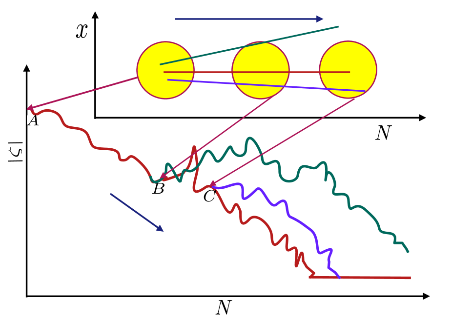
Figure 7: A schematic visualisation of change in coarse-grained curvature perturbation with e-folds $N$. The bottom graphs represents value of coarse-grained $\zeta$ at different spatial points. Initially, at $A$, a set of spatial points lie inside same the Hubble radius of the central point, whose evolution with time is red, inside which the white noises are correlated. The green and blue lines show branching evolution of the other points with time. After a certain instant, at points $B$ and $C$ different points move out the initial Hubble radius and experience the white noises to act differently in the future.

The $\delta N$-formalism [238, 239, 240, 241, 242, 243, 244, 245, 246, 247, 248, 249, 250, 251, 252, 253, 254, 255, 256, 257, 258, 259] has emerged as an important method to compute cosmological correlations in the super-Hubble scales and has found interesting applications in the framework of stochastic inflation [260, 261, 262, 263, 229, 264, 265, 266, 207, 267, 55, 268, 269, 270, 271, 52, 272, 273, 43, 274, 231, 275, 276, 262] since it is able to directly relate the probability distribution of the stochastic e-folding variable ${\cal N}$ to the statistics of the curvature perturbation variable $\zeta$. The fluctuations in the e-folds across different patches of homogeneous FLRW Universes are, at leading order, related to the amount of curvature perturbations generated at some final time, usually chosen late in the super-Hubble scales.

Generally, we start with the assumption of an unperturbed, locally homogeneous, and isotropic spacetime governed by the metric:

$$ds^{2}=-dt^{2}+a^{2}(t)\delta_{ij}dx^{i}dx^{j},$$ (213)

where $t$ is the cosmic time and $a(t)\sim\exp(Ht)$ (where $\dot{H}\neq 0$ so that $\epsilon=-\dot{H}/H^{2}$ exists). In the unperturbed Universes case, the Hubble parameter remains the only scale of interest to work in. In the presence of some kind of smoothing, on the scales of order $k^{-1}$, any quantity of interest is assumed to be sufficiently smooth. The perturbations come into the picture when the associated coordinate scale $k^{-1}$ becomes close to the Hubble radius, $k\sim aH$, and thereby the resulting anisotropies can appear perturbatively in powers of ${\cal O}(k/aH)$.

Next, we consider removing the gauge redundancies by the choice of a certain gauge. An example of this is choosing the uniform density gauge where the spatial slices of fixed time $t$ have uniform energy density. This choice then allows one to write the perturbed metric, considering only the scalar perturbations at this level, as follows:

$$ds^{2}=-dt^{2}+a^{2}(t)e^{2\zeta(t,{\bf x})}dx^{i}dx^{j},$$ (214)

where the new variable $\zeta(t,{\bf x})$ is the curvature perturbation present throughout our observable Universe. The form of the above-perturbed metric allows one to introduce a local scale factor consisting of a global time-dependent part and the perturbation as $\tilde{a}(t,{\bf x})=a(t)e^{2\zeta(t,{\bf x})}$. Using this new scale factor, we can introduce the amount of expansion realised when going from an initially flat, constant $t=t_{i}$ hypersurface ($\Omega_{i}$) to a final, constant $t$ hypersurface ($\Omega_{f}$) assigned with some uniform-density as:

$$N(t,{\bf x})=\ln{\bigg{(}\frac{\tilde{a}(t,{\bf x})}{a(t_{i})}\bigg{)}}.$$ (215)

The above can then be used to write down the amount of curvature perturbation experienced at a spatial point $x_{i}$, at instant $t$ in relation with the e-foldings elapsed upto that instant as follows:

$$\zeta(t,{\bf x}_{i})=N(t,{\bf x}_{i})-\bar{N}(t),\quad\quad\text{where}\;\bar{N}(t)=\ln{\bigg{(}\frac{a(t)}{a(t_{i})}\bigg{)}},$$ (216)

where the bar notation denotes the unperturbed amount of expansion, while $N(t,{\bf x}_{i})$ denotes the amount of expansion for unperturbed, FLRW Universes.

We now briefly talk about the stochastic formalism in inflation and the benefits of integrating it with the aforementioned $\delta N$-formalism. Here we consider not one but instead a family of FLRW Universes evolving from a certain initial condition on the phase space variables. These variables can be combined in form of a phase space vector ${\Gamma}_{i}=\{\zeta_{i},\Pi_{\zeta,i}\}$ where the index $i$ labels the various components. In the language of curvature perturbation, the stochastic formalism consists of constructing a low-energy effective theory of the long-wavelength or IR part of the initial primordial fluctuations. These fluctuations are coarse-grained over a certain fixed scale, close to the Hubble radius and defined as $k_{\sigma}=\sigma aH$, where $\sigma\ll 1$, and the resulting scalar curvature perturbation reads:

$$\zeta_{\rm cg}({\bf x})=\int_{\mathbb{R^{3}}}\frac{d^{3}k}{(2\pi)^{3}}\zeta_{k}e^{-i{\bf k}.{\bf x}},$$ (217)

where integration consider modes with wavenumber $k<k_{\sigma}$, or the IR modes in the coarse-grained curvature perturbation. As the Horizon size continues to decrease, more and more short-scale modes participate in the region of stochastic effects, getting ‘classicalized’, and finally entering into the IR sector. The result is the appearance of classical noises, which then act on the dynamics of the super-Hubble modes, which are described by the Langevin equation; see section III.1 for a discussion on the UV and IR separation of the modes and derivation of the Langevin equation in the present context. The noises become correlated only when within the Hubble radius, highlighting the Markovian nature of the noises, and over which the spatial points start to evolve independently of each other with different noises, and a consequence of this is the existence of fluctuations in the number of e-folds realised for each point.

For now, we focus on a single spatial point. The amount of realised along the worldline trajectory of the single point, starting from some initial condition to a final hypersurface, becomes a stochastic variable, represented using ${\cal N}$. From the $\delta N$-formalism mentioned earlier in this section, one can relate the curvature perturbation produced at some spatial point, coarse-grained between the scale crossing at some initial conformal time $\tau_{i}$ and the scale crossing out at the final conformal time $\tau_{f}$, to the perturbation in the e-folding realised along the same worldline in between $\tau_{i}$ and $\tau_{f}$ as follows:

$$\zeta_{\rm cg}({\bf x})={\cal N}({\bf x})-\langle{\cal N}\rangle=\delta{\cal N},$$ (218)

where the angle brackets denote the statistical average after solving the Langevin equation for multiple realisations at a given spatial point. We reiterate that due to random noises, the e-folds realised automatically receive fluctuations, leaving ${\cal N}$ as a stochastic variable whose statistical properties can later be estimated. These fluctuations are nothing but the comoving curvature perturbation produced at the final hypersurface as consequence of the $\delta N$-formalism. The fig. 7 describes the evolution of the spatial points during inflation and the instances where the Gaussian random noises start to affect the points separately, at $B$ and $C$ in the figure. The coarse-grained value of the curvature perturbation remains the same at all spatial points inside a Hubble patch (yellow circles) starting from points $A$ up to $B$ and $C$ after which they evolve in a statistically independent manner (shown in green and blue lines).

Comparison between the $\delta N$ (without stochasticity) and Stochastic-$\delta N$ formalism
	$\delta N$-formalism	Stochastic-$\delta N$ formalism
$1).$	e-folds of evolution vary ($\delta N$) for each point $(\bf{x})$	e-folds for a specific point $(\bf{x})$ on the final slice
	on the final hypersurface slice.	receive quantum fluctuations throughout evolution.
$2).$	Curvature perturbations on the final slice	Curvature perturbations requires coarse-graining
	directly related to $\delta N$ in the super-Horizon.	before relating to e-folds statistics in the super-Horizon.
$3).$	$\zeta(t,{\bf x}_{i})=N(t,{\bf x}_{i})-\bar{N}(t)=\delta N$,	$\zeta_{\rm cg}({\bf x})={\cal N}({\bf x})-\langle{\cal N}\rangle=\delta{\cal N}$,
	$N$: e-fold amount for expanding FLRW Universes	${\cal N}$: stochastic variable under Langevin equations for $\zeta_{\rm cg}(\bf{x})$
$4).$	No influence of quantum noises on evolution history.	Quantum noises classicalize after cut-off and affect $\zeta_{\rm cg}$ evolution.

Table 1: Comparative study between the two frameworks: $\delta N$ (without stochasticity) and stochastic-$\delta N$.

Table 1 summarizes the key differences between the usual $\delta N$ (without stochasticity) and the stochastic-$\delta N$ formalism. From the above discussion, we outline how the power of the $\delta N$-formalism can be utilised with stochastic formalism instead of solving the Langevin equation over multiple spatial points. The power spectrum $\Delta^{2}_{f,g}$ is an example of a quantity easily estimated from this stochastic-$\delta N$ formalism which we now mention. Here $\{f,g\}$ refer to the phase space variables $\{\zeta,\Pi_{\zeta}\}$, and using Fourier mode decomposition, the dimensionless power spectrum for the e-folding fluctuation $\delta N$ can be written down as:

$$\Delta^{2}_{\delta N}(k)=\frac{k^{3}}{2\pi^{2}}\int\;d^{3}{\bf x}\int\;d^{3}{\bf x^{\prime}}\langle\delta N({\bf x^{\prime}})\delta N({\bf x})\rangle e^{-i{\bf k}.({\bf x}-{\bf x^{\prime}})},$$ (219)

which can be inverted to give the variance in e-folds as:

$$\langle\delta{\cal N}^{2}\rangle=\langle({\cal N}-\langle{\cal N}\rangle)^{2}\rangle=\langle{\cal N}^{2}\rangle-\langle{\cal N}\rangle^{2} = \int\frac{d^{3}{\bf k}}{(2\pi)^{3}}\int\frac{d^{3}{\bf k^{\prime}}}{(2\pi)^{3}}\langle\delta N_{\bf k}\delta N_{\bf k^{\prime}}\rangle$$ (220)

$$= \int\frac{d^{3}{\bf k}}{(2\pi)^{3}}\int\frac{dk^{\prime}}{k^{\prime}}\frac{k^{\prime 3}}{2\pi^{2}}\langle\delta N_{\bf k}\delta N_{\bf k^{\prime}}\rangle$$

$$= \int\frac{d^{3}{\bf k}}{(2\pi)^{3}}\int\frac{dk^{\prime}}{k^{\prime}}\Delta^{2}_{\delta N}(k^{\prime})\delta^{(3)}({\bf k}+{\bf k^{\prime}})$$

$$= \int_{k}^{k_{f}}\frac{dk}{k}\Delta^{2}_{\delta N}(k)$$

$$= \int_{\ln{k_{f}}-\langle{\cal N}\rangle}^{\ln{k_{f}}}\Delta^{2}_{\delta N}(N)dN,$$

where we implement the definition of the power spectrum in the second line and in the last equality conversion is done using $\ln{(k)}=\ln{(aH)}$, for some wavenumber $k=|{\bf k}|$, and the fact that the average e-foldings is equal to $\langle{\cal N}\rangle=\ln{(a_{f}H/aH)}=\ln{(k_{f}/k)}$ assuming constant Hubble parameter $H$. The variance on the left is a statistical quantity and involves the average of the stochastic variable, $\langle{\cal N}\rangle$, in the right. From the above one can finally write down the dimensionless power spectrum for the curvature perturbation as:

$$\Delta^{2}_{\zeta\zeta}(k)=\Delta^{2}_{\delta N}(k)=\frac{d}{d\langle{\cal N}\rangle}\langle\delta{\cal N}^{2}\rangle\big{|}_{\langle{\cal N}\rangle=\ln{(k_{f}/k)}},$$ (221)

where the first equality follows from eqn. (218), and the above uses all the modes $k$ crossing out the Hubble radius between some initial instant and the end of inflation. In a similar fashion, we can further write down, using the higher-order statistical moments of $\langle\delta{\cal N}\rangle$, various other higher-order correlation functions. The local non-gaussianity is generally described in form of an expansion ansatz for the curvature perturbation $\zeta({\bf x})$ in the position space and around a Gaussian component:

$$\zeta({\bf x})=\zeta_{g}({\bf x})+\frac{3}{5}f_{\rm NL}\zeta^{2}_{g}({\bf x})+\frac{9}{25}g_{\rm NL}\zeta^{3}_{g}({\bf x})+{\cal O}(\zeta^{4}_{g}({\bf x}))+\cdots,$$ (222)

$\zeta_{g}({\bf x})$ where is the perturbation component obeying Gaussian statistics. Our interest lies in estimating the above introduced various non-Gaussian parameters, mainly $f_{\rm NL},g_{\rm NL},\tau_{\rm NL}$, using statistics of the e-folds ${\cal N}$ and the stochastic-$\delta N$ formalism.

Consider the case of the bispectrum and non-Gaussianity parameter $f_{\rm NL}$. The bispectrum is defined in relation with the three-point correlation function $\langle\zeta_{\bf k_{1}}\zeta_{\bf k_{2}}\zeta_{\bf k_{3}}\rangle$. Just like the inverse Fourier mode of the power spectrum is related to the variance, as in eqn. (220), a similar treatment for the bispectrum, this time doubly integrated, results in the third-moment of the e-folds $\langle\delta{\cal N}^{3}\rangle$. To show this, we can write:

$$\langle\delta{\cal N}^{3}\rangle=\langle({\cal N}-\langle{\cal N}\rangle)^{3}\rangle = \langle{\cal N}^{3}\rangle-3\langle{\cal N}\rangle\langle{\cal N}^{2}\rangle+2\langle{\cal N}\rangle^{3}$$ (223)

$$= \int\frac{d^{3}{\bf k_{1}}}{(2\pi)^{3}}\int\frac{d^{3}{\bf k_{2}}}{(2\pi)^{3}}\int\frac{d^{3}{\bf k_{3}}}{(2\pi)^{3}}\langle\delta N_{\bf k_{1}}\delta N_{\bf k_{2}}\delta N_{\bf k_{3}}\rangle,$$

$$= \int\frac{d^{3}{\bf k_{1}}}{(2\pi)^{3}}\int\frac{d^{3}{\bf k_{2}}}{(2\pi)^{3}}\int\frac{d^{3}{\bf k_{3}}}{(2\pi)^{3}}(2\pi)^{3}{\cal B}_{\delta N}(k_{1},k_{2},k_{3})\delta^{(3)}({\bf k_{1}}+{\bf k_{2}}+{\bf k_{3}}),$$

$$= \int\frac{d^{3}{\bf k_{1}}}{(2\pi)^{3}}\int\frac{d^{3}{\bf k_{2}}}{(2\pi)^{3}}{\cal B}_{\delta N}(k_{1},k_{2},k_{3})\big{|}_{{\bf k_{1}}+{\bf k_{2}}+{\bf k_{3}}=0},$$

which involves further volume integral over a tetrahedral region due to triangular constraint from the delta function. However, for our current purpose, we observe that the third moment of e-folds $\langle\delta{\cal N}^{3}\rangle$ receives twice the integrated contribution from the bispectrum. Thus, again using eqn. (218), we can write the expression for the Bispectrum:

$${\cal B}_{\zeta\zeta\zeta}(k_{1},k_{2},k_{3})\propto\frac{d\langle\delta{\cal N}^{3}\rangle^{2}}{d\langle{\cal N}\rangle^{2}},$$ (224)

Now, the parameter $f_{\rm NL}$ and the bispectrum are related to each other as follows:

$${\cal B}_{\zeta\zeta\zeta}(k_{1},k_{2},k_{3})=\frac{6}{5}f_{\rm NL}\left[\Delta^{2}_{\zeta\zeta}(k_{1})\Delta^{2}_{\zeta\zeta}(k_{2})+\Delta^{2}_{\zeta\zeta}(k_{1})\Delta^{2}_{\zeta\zeta}(k_{3})+\Delta^{2}_{\zeta\zeta}(k_{2})\Delta^{2}_{\zeta\zeta}(k_{3})\right],$$ (225)

from where one can consider for $f_{\rm NL}$ using eqn. (221) the relation:

$$f_{\rm NL}=\frac{5}{36}\frac{d\langle\delta{\cal N}^{3}\rangle^{2}}{d\langle{\cal N}\rangle^{2}}\big{(}\Delta^{2}_{\zeta\zeta}(k)\big{)}^{-2}=\frac{5}{36}\frac{d\langle\delta{\cal N}^{3}\rangle^{2}}{d\langle{\cal N}\rangle^{2}}\bigg{(}\frac{d\langle\delta{\cal N}^{2}\rangle}{d\langle{\cal N}\rangle}\bigg{)}^{-2},$$ (226)

which is a ratio of the bispectrum and the power spectrum squared, with the outside factor of $5/36$ coming from convention. The definition of the trispectrum involves, in a similar manner, the fourth moment of the e-folds $\langle\delta{\cal N}^{4}\rangle$ and taking its third derivative with respect to $\langle{\cal N}\rangle$, since it now receives thrice the integrated contributions. It is related to the four-point correlation function, $\langle\zeta_{\bf k_{1}}\zeta_{\bf k_{2}}\zeta_{\bf k_{3}}\zeta_{\bf k_{4}}\rangle$, and for this we start with the fourth moment of e-folds:

$$\langle\delta{\cal N}^{4}\rangle=\langle({\cal N}-\langle{\cal N}\rangle)^{4}\rangle = \langle{\cal N}^{4}\rangle-4\langle{\cal N}\rangle\langle{\cal N}^{3}\rangle+6\langle{\cal N}\rangle^{2}\langle{\cal N}^{2}\rangle-3\langle{\cal N}\rangle^{4},$$ (227)

$$= \int\frac{d^{3}{\bf k_{1}}}{(2\pi)^{3}}\int\frac{d^{3}{\bf k_{2}}}{(2\pi)^{3}}\int\frac{d^{3}{\bf k_{3}}}{(2\pi)^{3}}\int\frac{d^{3}{\bf k_{4}}}{(2\pi)^{3}}\langle\delta N_{\bf k_{1}}\delta N_{\bf k_{2}}\delta N_{\bf k_{3}}\delta N_{\bf k_{4}}\rangle,$$

$$= \int\frac{d^{3}{\bf k_{1}}}{(2\pi)^{3}}\int\frac{d^{3}{\bf k_{2}}}{(2\pi)^{3}}\int\frac{d^{3}{\bf k_{3}}}{(2\pi)^{3}}\int\frac{d^{3}{\bf k_{4}}}{(2\pi)^{3}}(2\pi)^{3}T_{\delta N}(k_{1},k_{2},k_{3},k_{4})\delta^{(3)}({\bf k_{1}}+{\bf k_{2}}+{\bf k_{3}}+{\bf k_{4}}),\quad\quad\quad$$

$$= \int\frac{d^{3}{\bf k_{1}}}{(2\pi)^{3}}\int\frac{d^{3}{\bf k_{2}}}{(2\pi)^{3}}\int\frac{d^{3}{\bf k_{3}}}{(2\pi)^{3}}T_{\delta N}(k_{1},k_{2},k_{3},k_{4})\big{|}_{{\bf k_{1}}+{\bf k_{2}}+{\bf k_{3}}+{\bf k_{4}}=0},$$

where have used the relation for the connected part of the four-point function. Now, the connected part of the trispectrum for the curvature perturbations is defined in combination of the power spectrum as follows:

$$T_{\zeta\zeta\zeta\zeta}(k_{1},k_{2},k_{3},k_{4}) = \tau_{\rm NL}\big{[}\Delta^{2}_{\zeta\zeta}(k_{13})\Delta^{2}_{\zeta\zeta}(k_{3})\Delta^{2}_{\zeta\zeta}(k_{4})+11\;\text{perms.}\big{]}$$ (228)

$$+\frac{54}{25}g_{\rm NL}\big{[}\Delta^{2}_{\zeta\zeta}(k_{2})\Delta^{2}_{\zeta\zeta}(k_{3})\Delta^{2}_{\zeta\zeta}(k_{4})+3\;\text{perms.}\big{]},$$

with the notation for magnitude $k_{ij}=|{\bf k}_{i}+{\bf k}_{j}|$ and the cubic dependence on the power spectrum being a reason behind its name as the trispectrum. We notice that there emerge two distinct non-linearity parameters from the connected part of the trispectrum, $\tau_{\rm NL}$ and $g_{\rm NL}$, based on their $k$ dependence. The $12$ permutations comes from having $3$ distinct choices for the indices in $k_{ij}$, as the magnitude remains same, $k_{ij}=k_{ji}$, and from the momentum conserving delta function we have $k_{12}=k_{34},\;k_{23}=k_{14},\;k_{13}=k_{24}$. The $4$ permutations are again result of the conservation of momentum. From eqns. (218,221,228), we can ultimately write the following relations for the non-Gaussianity parameters in terms of the derivatives of the fourth moment:

$$\tau_{\rm NL} = \frac{1}{36}\bigg{(}\frac{d^{2}\langle\delta{\cal N}^{3}\rangle}{d\langle{\cal N}\rangle^{2}}\bigg{)}^{2}\big{(}\Delta^{2}_{\zeta\zeta}(k)\big{)}^{-4}=\frac{1}{36}\bigg{(}\frac{d^{2}\langle\delta{\cal N}^{3}\rangle}{d\langle{\cal N}\rangle^{2}}\bigg{)}^{2}\bigg{(}\frac{d\langle\delta{\cal N}^{2}\rangle}{d\langle{\cal N}\rangle}\bigg{)}^{-4},$$ (229)

$$g_{\rm NL} = \frac{d\langle\delta{\cal N}^{4}\rangle^{3}}{d\langle{\cal N}\rangle^{3}}\big{(}\Delta^{2}_{\zeta\zeta}(k)\big{)}^{-3}=\frac{d\langle\delta{\cal N}^{4}\rangle^{3}}{d\langle{\cal N}\rangle^{3}}\bigg{(}\frac{d\langle\delta{\cal N}^{2}\rangle}{d\langle{\cal N}\rangle}\bigg{)}^{-3},$$ (230)

where the factor $1/36$ again results from convention purposes.

Now that we have laid out the stochastic-$\delta N$ formalism in the context of EFT of single field inflation, and its applications into calculating higher-order correlation functions, we make use of the above developments to understand the probability distribution driving the duration of inflation. Computation of this distribution has major advantages in terms of knowing the mass fraction of the PBH when focusing on the diffusion dominated regime of inflation and identifying the non-Gaussianity parameters when focusing on the drift-dominated regime during inflation. We aim to perform these calculations in the EFT picture coupled with the stochastic-$\delta N$ formalism.

VIII Probability Distribution Function from Fokker-Planck equation

In this section, we derive the Fokker-Planck equation in its complete form which will later help us to analyze the probability distribution functions. The Fokker-Planck equation allows us to study the evolution of the probability density function from one point to another in the field space and here it is defined for the stochastic e-folds variable ${\cal N}$ elapsed between the start and end of the evolution. It involves the adjoint Fokker-Planck operator acting on the probability distribution function $P_{\bf\Gamma}({\cal N})$ in the following manner:

$$\frac{\partial}{\partial{\cal N}}P_{\bf\Gamma}({\cal N})=\Bigg{(}F_{i}\frac{\partial}{\partial\Phi_{i}}+\frac{1}{2}\Sigma_{ij}\frac{\partial^{2}}{\partial\Gamma_{i}\partial\Gamma_{j}}\Bigg{)}P_{\bf\Gamma}({\cal N}),$$ (231)

where the Adjoint Fokker-Planck operator can be expanded as follows:

$$F_{i}\frac{\partial}{\partial\Gamma_{i}}+\frac{1}{2}\Sigma_{ij}\frac{\partial^{2}}{\partial\Gamma_{i}\partial\Gamma_{j}} = \Pi_{\zeta}\frac{\partial}{\partial\zeta}-(3-\epsilon)\Pi_{\zeta}\bigg{[}1-\frac{2(s-\frac{\eta}{2})}{3-\epsilon}\bigg{]}\frac{\partial}{\partial\Pi_{\zeta}}$$ (232)

$$\quad\quad\quad\quad\quad\quad\quad+\frac{1}{2}\bigg{(}\Sigma_{\zeta\zeta}\frac{\partial^{2}}{\partial\zeta^{2}}+\Sigma_{\zeta\Pi_{\zeta}}\frac{\partial^{2}}{\partial\zeta\partial\Pi_{\zeta}}+\Sigma_{\Pi_{\zeta}\zeta}\frac{\partial^{2}}{\partial\Pi_{\zeta}\partial\zeta}+\Sigma_{\Pi_{\zeta}\Pi_{\zeta}}\frac{\partial^{2}}{\partial\Pi_{\zeta}\partial\Pi_{\zeta}}\bigg{)}.$$

At this stage we use the super-Hubble conditions, $\sigma\ll 1$, for examining this equation which renders the noise matrix elements $\Sigma_{\zeta\Pi_{\zeta}},\;\Sigma_{\Pi_{\zeta}\zeta},\Sigma_{\Pi_{\zeta}\Pi_{\zeta}}$ almost negligible. Next, to further simplify the representation of this Fokker-Planck operator, we employ the following re-scaling of the coarse-grained variables $\{\zeta,\Pi_{\zeta}\}$ into the new variables:

$$\zeta=f,\quad\quad\Pi_{\zeta}=-3y,$$ (233)

using this we observe the following transformation of various other differential operators present:

$$\frac{1}{2}\Sigma_{\zeta\zeta}\frac{\partial^{2}}{\partial\zeta^{2}}=\frac{1}{\mu^{2}}\frac{\partial^{2}}{\partial f^{2}},$$ (234)

$$\Pi_{\zeta}\frac{\partial}{\partial\Pi_{\zeta}}=y\frac{\partial}{\partial y},$$ (235)

$$\Pi_{\zeta}\frac{\partial}{\partial\zeta}=-3y\frac{\partial}{\partial f}.$$ (236)

With the new re-scaled variables in hand, we rewrite the Fokker-Planck operator as:

$$\frac{\partial}{\partial\mathcal{N}}P_{\bf\Gamma}(\mathcal{N}) = \bigg{[}\frac{1}{\mu^{2}}\frac{\partial^{2}}{\partial f^{2}}-3\bigg{\{}y\frac{\partial}{\partial f}+\bigg{(}1-\frac{\epsilon}{3}\bigg{)}\bigg{(}1-\frac{2(s-\frac{\eta}{2})}{3-\epsilon}\bigg{)}y\frac{\partial}{\partial y}\bigg{\}}\bigg{]}P_{\bf\Gamma}({\cal N}),$$ (237)

in which, for clarity, we further perform another set of following re-definitions:

$$C=\bigg{(}1-\frac{\epsilon}{3}\bigg{)}\bigg{(}1-\frac{2(s-\frac{\eta}{2})}{3-\epsilon}\bigg{)},\quad\quad Cf=x,\quad\quad\left(\frac{C}{\mu}\right)^{2}=\frac{1}{\tilde{\mu}^{2}}$$ (238)

and these changes ultimately gives rise to the Fokker-Planck equation version of our interest:

$$\frac{\partial}{\partial\mathcal{N}}P_{\bf\Gamma}(\mathcal{N}) = \bigg{[}\frac{1}{\tilde{\mu}^{2}}\frac{\partial^{2}}{\partial x^{2}}-3Cy\bigg{\{}\frac{\partial}{\partial x}+\frac{\partial}{\partial y}\bigg{\}}\bigg{]}P_{\bf\Gamma}({\cal N}).$$ (239)

Notice that the changes coming from an underlying EFT setup are contained within the coefficient $C$, which we now refer to as the characteristic parameter, and it will have noticeable changes when we understand the probability distribution evolution in the next section. Also, the change from $C$ is felt by the coefficient $\mu$ containing the auto-correlated power spectrum element for $\zeta$. In the case where $C=1$ reduces to the canonical single-field inflation scenario while for $C\neq 1$ we are working with the non-canonical single-field models of inflation. In the next section, we explore the method that will enable us to calculate this PDF depending on the interested conditions for a general EFT setup.

IX Characteristic function and Initial Conditions

In the stochastic inflation framework, our stochastic variable of interest is the e-folds ${\cal N}$, and for this, we have seen the evolution of the corresponding PDF governed by the Fokker Planck equation. To fully determine the nature of this PDF, one requires information on its associated moments as they dictate the statistical properties of this PDF. Here, we discuss the method of the characteristic function that will let us evaluate the moments of arbitrary degree for a given PDF, $P_{\Gamma_{i}}({\cal N})$, and would also manage to reconstruct the entire PDF.

The characteristic function converts the probability distribution from a function of $3$ variables, in the phase space ${\Gamma_{i}}=\{\zeta,\Pi_{\zeta}\}$ and the variable ${\cal N}$, to a function of just the phase space variables ${\Gamma_{i}}$. It is defined as the Fourier transform of the original PDF in the ${\cal N}$ co-ordinate as:

$$\chi(t;x,y)=\int_{-\infty}^{+\infty}e^{it{\cal N}}P_{{\Gamma_{i}}}({\cal N})d{\cal N},$$ (240)

where $t$ acts as a dummy variable which is a complex quantity in general. This function $\chi(t;{\Gamma_{i}})$ is useful to provide the various statistical moments associated with the full PDF $P_{\Gamma_{i}}({\cal N})$. Inversely, one can obtain the PDF from the characteristic function as follows:

$$P_{{\Gamma_{i}}}({\cal N})=\frac{1}{2\pi}\int_{-\infty}^{+\infty}e^{-it{\cal N}}\chi(t;{\Gamma_{i}})dt.$$ (241)

The corresponding information for the moments can be extracted by Taylor expanding $\chi(t;{\Gamma_{i}})$ around $t=0$ and observing that:

$$\chi(t;{\Gamma_{i}})=\sum_{n=0}^{\infty}\frac{(it)^{n}}{n!}\langle{\cal N}^{n}({\Gamma_{i}})\rangle\implies\langle{\cal N}^{n}({\Gamma_{i}})\rangle=i^{-n}\frac{\partial^{n}}{\partial t^{n}}\chi(t;{\Gamma_{i}})|_{t=0},$$ (242)

where the index $n$ denotes the $n$th moment, $\langle{\cal N}^{n}({\Gamma_{i}})\rangle$, of the full PDF. By using the definition of PDF from eqn. (241), into the Fokker-Planck eqn. (239), one also notices that the characteristic function obeys:

$$\bigg{[}\frac{1}{\tilde{\mu}^{2}}\frac{\partial^{2}}{\partial x^{2}}-3Cy\bigg{\{}\frac{\partial}{\partial x}+\frac{\partial}{\partial y}\bigg{\}}+it\bigg{]}\chi(t;{\Gamma_{i}})=0.$$ (243)

The solution of this equation leads us to identify the function $\chi(t;{\Gamma_{i}})$. In the next sections, we will analyze the characteristic function solutions under specific conditions for the $y$ parameter and in the presence of certain boundary conditions needed to sufficiently handle the above two-dimensional partial differential equation.

X Diffusion Dominated Regime: Methods to solve for the Characteristic function

In this section, we concern ourselves with the regime where quantum diffusion effects dominate the dynamics. This regime is also where the conjugate momentum variable, see eqn.(233), takes on very small values, $0<y\ll 1$. This regime is significant from the perspective of analyzing PBH more accurately since we will observe distinctive features in the upper tail of the PDF, which is precisely the region of importance for the formation of PBH. Also, it can be seen from the perspective of the conjugate field momenta since it decreases in this regime, and thus, diffusion effects primarily govern the behaviour of the scalar perturbations and features of the PDF.

To generate the PDF requires solving the partial differential equation in eqn.(243). We solve first for the characteristic function $(\chi)$ which will then help us to build the PDF and the related methodology is the subject of this section.

To this effect, we start with a particular variable re-definition:

$$u=x-y,\quad\quad\quad v=y,$$ (244)

that simplifies the equation for the characteristic function as follows:

$$\bigg{[}\frac{1}{\tilde{\mu}^{2}}\frac{\partial^{2}}{\partial u^{2}}-3Cv\frac{\partial}{\partial v}+it\bigg{]}\chi(t;u,v)=0.$$ (245)

The above equation is now made separable in its variables and thus accepts an ansatz of the form:

$$\chi(t;u,v)=\sum_{n=0}^{\infty}v^{n}U_{n}(t;u),$$ (246)

and here we further utilize the fact visible from the structure of the new partial differential equation, eqn.(245), that the function $R(t;r)$ admits oscillatory solutions that follow:

$$\frac{\partial^{2}}{\partial r^{2}}U_{n}(t;u)+\omega_{n}^{2}(t)U_{n}(t;u)=0,$$ (247)

where the frequency contains the effects from the EFT parameter as:

$$\omega_{n}^{2}(t)=(it-3Cn)\mu^{2}.$$ (248)

Now, in order to fully utilize the ansatz and determine $\chi(t;u,v)$, we implement the appropriate boundary conditions that can describe the behaviour of the perturbations as they enter and exit the diffusion-dominated regime. The first case corresponds to the condition where the perturbations are almost unaffected by quantum diffusion processes with the perturbations still not present under the influence of the USR, conversely, the second case is where the diffusion effects dominate the overall dynamics and dictate the behaviour of the PDF for large values of the perturbations. The above described conditions for the transformed phase space variables ${\Gamma_{i}}=\{u,v\}$ are written using the characteristic function as follows:

$$\underline{\bf Boundary\;Condition\;I:}\quad\quad\quad\quad\chi(t;\Gamma_{i})|_{u+v=0}=1,$$ (249)

$$\underline{\bf Boundary\;Condition\;II:}\quad\quad\quad\left.\frac{\partial\chi(t;\Gamma_{i})}{\partial u}\right|_{u+v=1}=0,$$ (250)

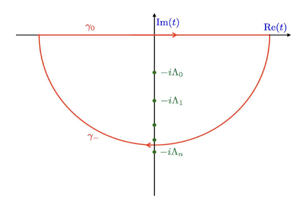
Figure 8: Closed contour $\gamma_{0}\cup\gamma_{-}$ in the complex plane containing poles of the characteristic function on the imaginary $t$ axis. The residue theorem when applied at these poles results into the PDF $P_{\Gamma}({\cal N})$.

where written for the new variables, $(u,v)$, these conditions concerns with the value of $\zeta$. The first condition refers to smaller values of $\zeta$ and conversely, the second condition refers to larger values of $\zeta$. However, the solution now involves mode mixing due to the nature of the conditions involving both new variables and we examine how these affect the solution from the series ansatz. Since it follows oscillatory behaviour, we can write the solution for the function $U_{n}(t;u)$ as:

$$U_{n}(t;u)=R_{n}(t)\cos{((1-u)\omega_{n}(t))}+Q_{n}(t)\sin{((1-u)\omega_{n}(t))},$$ (251)

and using this solution with the conditions from eqn.(249) and eqn.(250), we get the following constraints on the series:

$$\sum_{n=0}^{\infty}v^{n}\big{[}R_{n}\cos{((1+v)\omega_{n}(t))}+Q_{n}(t)\sin{((1+v)\omega_{n}(t))}\big{]}=1,$$

$$\sum_{n=0}^{\infty}\omega_{n}v^{n}\big{[}R_{n}\sin{(\omega_{n}v)}-Q_{n}\cos{(\omega_{n}v)}\big{]}=0.$$ (252)

From this, by series expanding the oscillatory functions, one can generate recurrence relations for the various coefficients $R_{n},\;Q_{n}$ for each order in index $n$. We conduct our analysis for each order in the series till we reach $n=3$ which allows us to construct the next-to-next-to-next leading order (NNNLO) version of the PDF and for that, we require the explicit form of these coefficients using the mentioned recurrence relations. We mention the coefficients up to $m=2$, or to construct the second order (NNLO) contribution, here as:

$$R_{0} = \frac{1}{\cos{(\omega_{0})}},$$

$$R_{1} = \frac{\omega_{0}}{\omega_{1}}\frac{\omega_{1}\sin{(\omega_{0})}-\omega_{0}\sin{(\omega_{1})}}{\cos{(\omega_{0})}\cos{(\omega_{1})}},$$

$$R_{2} = \frac{\omega_{1}\sin{(\omega_{1})}P_{1}-\omega_{1}\cos{(\omega_{1})}Q_{1}-\sin{(\omega_{2})}Q_{2}+\frac{\omega_{0}^{2}}{2}\cos{(\omega_{0})}P_{0}}{\cos{(\omega_{2}})},$$ (253)

and

$$Q_{0} = 0,$$

$$Q_{1} = \frac{\omega_{0}^{2}}{\omega_{1}}P_{0},$$

$$Q_{2} = \frac{\omega_{1}^{2}}{\omega_{2}}P_{1},$$ (254)

and those for the third order are mentioned in the next section dedicated to NNNLO.

We follow the approach in [38] of writing the characteristic function in a series expansion of the following form:

$$\chi(t;{\Gamma_{i}})=\sum_{m}\sum_{n}\frac{r_{n}^{(m)}({\Gamma_{i}})}{\Lambda_{n}^{(m)}-it}+h(t;{\Gamma_{i}}),$$ (255)

where the use of ${\Gamma_{i}}$ highlights the dependence of the residues on the phase space variables, or the initial conditions, and the poles, $\Lambda_{n}^{(m)}$, always remain independent of the set of values in ${\Gamma_{i}}$, which we will show in the next step. The function $h(t;{\Gamma_{i}})$ is the regular part of the expansion and would not contribute in the later discussions as we will show. The fig. 8 illustrates the application of residue theorem at the poles located on the imaginary $t$-axis enclosed by a contour $\gamma_{0}\cup\gamma_{-}$. As seen from their expressions above, the terms $R_{n},\;Q_{n}$ admits simple poles in their structure and thus, for the characteristic function $\chi(t;{\Gamma_{i}})$, an expansion of the type in eqn.(255) works for our purpose. The poles correspond to the condition:

$$\cos{(\omega_{m}(t))}=0,\quad\quad\text{hence,}\quad\omega_{m}(t)=\left(n+\frac{1}{2}\right)\pi,$$ (256)

where the integer $n$ labels the number of distinct positions we have a pole of the $m$th order. The above equation from the use of eqn. (248) can be converted to give the pole expression as:

$$\Lambda_{n}^{(m)}=3Cm+\bigg{[}\frac{\pi}{\tilde{\mu}}\left(n+\frac{1}{2}\right)\bigg{]}^{2},$$ (257)

and here we can notice the impact of the characteristic parameter, see eqn.(238). Another quantity of importance are the residues, represented here by $r_{n}^{(m)}({\Gamma_{i}})$, and these are evaluated by inverting the expression in eqn.(255) and taking the time-derivative in the following manner:

$$r_{n}^{(m)}({\Gamma_{i}})=-i\bigg{[}\left.\frac{\partial}{\partial t}\chi^{-1}(t;{\Gamma_{i}})\right|_{t=-i\Lambda_{n}^{(m)}}\bigg{]}^{-1},$$ (258)

The above information regarding the poles and the residues combine together to construct the PDF if we use the eqn.(255) with the Fourier transform expression in eqn.(241), which results in:

$$P_{\Gamma_{i}}({\cal N})=\sum_{m=0,1,\cdots}\sum_{n=0}^{\infty}r_{n}^{(m)}({\Gamma_{i}})\exp{(-\Lambda_{n}^{(m)}{\cal N})}.$$ (259)

with the outside sum going up to the desired order $m$th order. The exponential decay of the PDF at each order in the expansion is determined by the value of the poles $\Lambda_{n}^{(m)}$ and, for large values of the e-folds ${\cal N}$ the dominant contribution solely comes from the lowest pole $\Lambda_{0}$ and it corresponding residue $r_{0}^{(m)}$. As mentioned earlier, the regular function in the expansion, eqn. (255), plays no role in determining the final PDF expansion. We can thus use the characteristic function and find its residues corresponding to the simple poles at each subsequent order in the expansion to construct, using the above, the full PDF at the $m$th order.

X.1 Calculation of PDF at LO

In this section, we discuss the calculation of the probability distribution at the leading order (LO) for the diffusion-dominated regime. We follow the approach described in the previous section based on the characteristic function and use its series expansion to find the residues and the corresponding decay factors involving the poles.

For the leading order, we only require to use the first set of coefficients, $(R_{0},Q_{0})$, in eqn. (X). These imply that the drift contributions are completely ignored since we are working in the limit where $(v\rightarrow 0,\;u\rightarrow x)$ and using the corresponding LO characteristic function we can proceed to find its PDF. The first job is to use the following function at LO:

$$\chi^{\rm LO}(t;x,0)=\frac{\cos{((1-x)\omega_{0})}}{\cos{(\omega_{0})}},$$ (260)

and find the residues using eqn. (258) using the $m=0$ poles, $\Lambda_{n}^{(0)}$, in eqn. (257). Notice here that the characteristic parameter $C$ for the EFT does not directly come into the picture at LO. The residues then obtained are given by,

$$r_{n,0}^{(m=0)}=(2n+1)\frac{\pi}{\tilde{\mu}^{2}}\sin{\bigg{(}(2n+1)\frac{\pi x}{2}\bigg{)}},$$ (261)

which combines into the eqn. (259) with the poles to give for the PDF,

$$P_{\Gamma_{i}}^{\rm LO}({\cal N}) = \sum_{n=0}^{\infty}r_{n,0}^{(m=0)}\exp{(-\Lambda_{n}^{(0)}{\cal N})}=-\frac{\pi}{2\tilde{\mu}^{2}}{\cal V}^{\prime}_{2}\bigg{(}\frac{\pi}{2}x,\exp{\bigg{(}-\frac{\pi^{2}}{\tilde{\mu}^{2}}{\cal N}\bigg{)}}\bigg{)},$$ (262)

where ${\cal V}_{2}$ represents the elliptic theta function,

$${\cal V}_{2}(\alpha,x)=2\sum_{n=0}^{\infty}x^{(n+\frac{1}{2})^{2}}\cos{((2n+1)\alpha)},$$ (263)

and the notation, ${\cal V}^{\prime}_{2}$, refers to the derivative of the function with respect to its first argument. Here, the contribution coming from $n=0$ dominates the most when ${\cal N}$ is taken very large. In similar fashion, we develop the PDF for the next-to-leading order (NLO). The first and second moments from the above PDF at the leading order can also be calculated using the relation in eqn. (242). The knowledge of $\langle{\cal N}\rangle$ will prove necessary when we concern ourselves with the primordial black hole abundance in the coming sections. The expression for these moments of the number of e-folds ${\cal N}$ at LO is given by

$$\langle{\cal N}(x,y=0)\rangle_{\rm LO} = \tilde{\mu}^{2}x\bigg{(}1-\frac{x}{2}\bigg{)},$$ (264)

$$\langle{\cal N}^{2}(x,y=0)\rangle_{\rm LO} = \frac{1}{3}\tilde{\mu}^{4}x(2-x^{2}+x^{3}),$$ (265)

One immediate effect is clear that the mean value is more sensitive to changes in $\tilde{\mu}$. To get a better picture of this sensitivity let us evaluate the variance in the leading order, which gives us:

$$\sigma_{\rm LO}^{2}=\langle{\cal N}^{2}(x,y=0)\rangle_{\rm LO}-\langle{\cal N}(x,y=0)\rangle_{\rm LO}^{2}=\frac{1}{6}\tilde{\mu}^{4}x(2+x^{2}-2x)(2-x),$$ (266)

The variance experiences increased sensitivity as $\tilde{\mu}$ is increased slightly.

X.2 Calculation of PDF at NLO

Here we determine the first sub-dominant correction to the pure diffusion limit result in the previous section. We require here to use the second set of coefficients, $(R_{1},Q_{1})$, in eqn. (X) to properly determine the characteristic function and subsequent residues at the next-to-leading order in our $y$-expansion. We have at NLO the following function:

$$\chi^{\rm NLO}(t;\Gamma_{i})=U_{0}(t;u)+vU_{1}(t;u),$$ (267)

and further utilising the formulas in eqns. (257,258) using the above characteristic function, we now mention the residues at each order with information up to the first order ${\cal O}(y)$, as follows:

$$r_{n,1}^{(m=0)} = (2n+1)\frac{\pi}{\tilde{\mu}^{2}}\bigg{[}\sin{\left((2n+1)\frac{\pi x}{2}\right)}-y(2n+1)\frac{\pi}{2}\cos{\left((2n+1)\frac{\pi x}{2}\right)}\bigg{]}$$ (268)

$$+ y(2n+1)\frac{\pi}{2}\frac{1}{\omega^{(0)}_{n,1}\cos{(\omega^{(0)}_{n,1})}}\bigg{[}\omega^{(0)}_{n,1}\cos{\omega^{(0)}_{n,1}(1-x)}-(-1)^{n}(2n+1)\frac{\pi}{2}\sin{(x\;\omega^{(0)}_{n,1})}\bigg{]},$$

where the notation for the zero-order frequency at NLO means:

$$\omega^{(0)}_{n,1}=\sqrt{\left(n+\frac{1}{2}\right)^{2}\pi^{2}-3C\tilde{\mu}^{2}},$$ (269)

the above residues come associated with the zero-order pole at NLO, $\Lambda_{n}^{(0)}$. Similarly, for the first order poles, $\Lambda_{n}^{(1)}$, the residues have the following structure:

$$r_{n,1}^{(m=1)} = \frac{(-1)^{n+1}2y}{\tilde{\mu}^{2}}\frac{\sin{\left((n+\frac{1}{2})\pi x\right)}}{\cos{\left(\sqrt{\left(n+\frac{1}{2}\right)^{2}\pi^{2}+3C\tilde{\mu}^{2}}\right)}}\bigg{[}\left(n+\frac{1}{2}\right)^{2}\pi^{2}+3C\tilde{\mu}^{2}$$ (270)

$$\quad\quad\quad\quad\quad-(-1)^{n}\frac{\pi}{2}(2n+1)\sqrt{\left(n+\frac{1}{2}\right)^{2}\pi^{2}+3C\tilde{\mu}^{2}}\sin{\bigg{(}\sqrt{\left(n+\frac{1}{2}\right)^{2}\pi^{2}+3C\tilde{\mu}^{2}}\bigg{)}}\bigg{]},$$

Combining together eqns.(268,270) into the final PDF from eqn.(259) gives

$$P_{\Gamma_{i}}^{\rm NLO}({\cal N})=\sum_{n=0}^{\infty}\big{[}r_{n,1}^{(m=0)}+r_{n,1}^{(m=1)}e^{-3C{\cal N}}\big{]}e^{-\Lambda_{n}^{(0)}{\cal N}},$$ (271)

where in addition to the set of poles for $m=0$, we have another version of poles,

$$\Lambda_{n}^{(1)}=3C+\Lambda_{n}^{(0)},$$ (272)

contributing to the decay rate. The presence of characteristic parameter $C$ also alters the decay feature depending on its value, which remains close to $1$. Similar to the case of LO, here also one can evaluate the first moment or mean number $\langle{\cal N}\rangle$ to get the following:

$$\langle{\cal N}(\Gamma)\rangle_{\rm NLO}=\tilde{\mu}^{2}x\bigg{(}1-\frac{x}{2}\bigg{)}+\tilde{\mu}^{2}y\bigg{(}x-1+\frac{\cosh{[\sqrt{3C}\tilde{\mu}(1-x)]}}{\cosh{[\sqrt{3C}\tilde{\mu}]}}-\frac{\sinh{[\sqrt{3C}\tilde{\mu}x]}}{\sqrt{3C}\tilde{\mu}\cosh{[\sqrt{3C}\tilde{\mu}]}}\bigg{)},$$ (273)

which contains the linear correction terms, that is upto ${\cal O}(y)$. We will use this expression in the upcoming sections for PBH analysis.

X.3 Calculation of PDF at NNLO

Here we discuss the calculation of the probability distribution at the next-to-next-leading order (NNLO) for the diffusion-dominated regime. This means we work with the series ansatz in eqn. (246) truncated upto the quadratic terms to find those respective corrections. We would require knowledge of the residues and the corresponding poles to begin. The last set of coefficients in eqn. (X), $(R_{2},Q_{2})$, will be of use here. The characteristic function at NNLO now has the form:

$$\chi^{\rm NLO}(t;\Gamma_{i})=U_{0}(t;u)+vU_{1}(t;u)+v^{2}U_{2}(t;u),$$ (274)

following this, the residues from eqn. (258) at orders $m=0,1,2$, each expanded upto the second order ${\cal O}(y^{2})$, is required to eventually construct the PDF. We do not explicitly mention the analytic form of each residue due to its overall complexity. However, the figures obtained for $P_{\Gamma_{i}}^{\rm NNLO}(\cal N)$ will be discussed in good detail in the numerical analysis section. The final form of the PDF can be combined into the following expression:

$$P_{\Gamma_{i}}^{\rm NNLO}({\cal N})=\sum_{n=0}^{\infty}\big{[}r_{n,2}^{(0)}+r_{n,2}^{(1)}e^{-3C{\cal N}}+r_{n,2}^{(2)}e^{-6C{\cal N}}\big{]}e^{-\Lambda_{n}^{(0)}{\cal N}},$$ (275)

Here also, we can calculate the corrections to the mean number of e-folds at NNLO following the eqn. (242) along with the characteristic function in the above eqn.(274). This gives us the following expression for the mean:

$$\langle{\cal N}(\Gamma)\rangle_{\rm NNLO} = \tilde{\mu}^{2}x\bigg{(}1-\frac{x}{2}\bigg{)}+\tilde{\mu}^{2}y(-1+x-y)+\frac{\tilde{\mu}^{2}y^{2}}{2}\bigg{(}\frac{\cosh{[\sqrt{6C}\tilde{\mu}(1-x)]}}{\cosh{[\sqrt{3C}\tilde{\mu}]}\cosh{[\sqrt{6C}\tilde{\mu}]}}\bigg{)}$$ (276)

$$\times\bigg{(}-2+\cosh{[\sqrt{3C}\tilde{\mu}]}+\sqrt{6C}\tilde{\mu}\sinh{[\sqrt{6C}\tilde{\mu}]}-(2\sqrt{3C}\tilde{\mu}^{2}+\sqrt{2}\sinh{[\sqrt{6C}\tilde{\mu}]})\sinh{[\sqrt{3C}\tilde{\mu}]}\bigg{)}$$

$$+\frac{\tilde{\mu}^{2}y^{2}}{\sqrt{2}}\frac{\sinh{[\sqrt{6C}\tilde{\mu}(1-x)]}}{\sqrt{3C}\tilde{\mu}^{2}}-\tilde{\mu}y\sinh{[\sqrt{3C}\tilde{\mu}(1-x+y)]}-\frac{\tilde{\mu}^{2}y^{2}}{\sqrt{2}}\sinh{[\sqrt{6C}\tilde{\mu}(1-x)]}\tanh{[\sqrt{3C}\tilde{\mu}]}$$

$$+\tilde{\mu}^{2}y\cosh{[\sqrt{3C}\tilde{\mu}(1-x+y)]}\bigg{(}\frac{1}{\cosh{[\sqrt{3C}\tilde{\mu}]}}-\frac{\tanh{[\sqrt{3C}\tilde{\mu}]}}{\sqrt{3C}\tilde{\mu}}\bigg{)},$$

where we consider terms only upto ${\cal O}(y^{2})$.

X.4 Calculation of PDF at NNNLO

To completely determine the PDF we would require the recurrence relation between the coefficients, which we now mention:

$$R_{3} = \frac{1}{\cos{(\omega_{3})}}\bigg{[}\frac{1}{2}\omega_{1}^{2}(R_{1}\cos{(\omega_{1})}+Q_{1}\sin{(\omega_{1})})+\omega_{2}R_{2}\sin{(\omega_{2})}-\frac{1}{6}\omega_{0}^{3}R_{0}\sin{(\omega_{0})}-\omega_{2}Q_{2}\cos{(\omega_{2})}-Q_{3}\sin{(\omega_{3})}\bigg{]},$$

$$Q_{3} = \frac{1}{\cos{(\omega_{3})}}\bigg{[}\omega_{2}^{2}R_{2}+\frac{1}{2}\omega_{1}^{3}Q_{1}-\frac{1}{6}\omega_{0}^{4}R_{0}\bigg{]},$$ (277)

where the simple pole due to $\cos{(\omega_{3})}$ at $t=-i\Lambda_{n}^{(3)}$ is explicit. Already we notice that the expressions quickly become more cumbersome as we go beyond NNLO and these together with the previous values of the coefficients in eqn.(X) make up the characteristic function that will be needed to build the complete NNNLO PDF utilizing eqs.(246), (258) and (259).

Regarding the poles, the index $m$ now runs from $m=0,1,2,3$ with the last $m=3$, or

$$\Lambda_{n}^{(3)}=\Lambda_{n}^{(0)}+3Cm,$$ (278)

providing the smallest order of contribution while the $m=0$ provides the dominant contribution, which seems more important as we approach large values of ${\cal N}$. We do not mention here the complete form of the residues, $r_{n}^{(m)}\;\forall\;m=0,1,2,3$, as they are extremely complicated and not illuminating by themselves, and thus, we only later show their contribution in the form of the PDF realized after estimating them. The final NNNLO PDF using eqn.(259) has the following form:

$$P_{\Gamma_{i}}^{\rm NNNLO}({\cal N})=\sum_{n=0}^{\infty}\big{[}r_{n,3}^{(0)}+r_{n,3}^{(1)}e^{-3C{\cal N}}+r_{n,3}^{(2)}e^{-6C{\cal N}}+r_{n,3}^{(3)}e^{-9C{\cal N}}\big{]}e^{-\Lambda_{n}^{(0)}{\cal N}}$$ (279)

The residues, especially the term $r_{n}^{(0)}$ controlling the amplitude, do depend on the initial phase space variables, ${\Gamma_{i}}$, while the decay from the dominant exponential, $\exp{(-\Lambda_{n}^{0}{\cal N})}$, is independent of the same. The formula in eqn. (257) also tells us that when $\tilde{\mu}\gtrsim 1$, the poles remain well-separated along the imaginary $t$-axis. Expression for the mean number of e-folds now becomes much lengthy and complicated, and it is represented by the following relation:

$$\langle{\cal N}(\Gamma)\rangle_{\rm NNNLO} = \frac{\tilde{\mu}^{2}}{2}\bigg{\{}1-(1-x+y)^{2}+\frac{12\tilde{\mu}^{2}y\left(\sqrt{3C\tilde{\mu}^{2}}-\sinh\big{[}\sqrt{3C\tilde{\mu}^{2}}\big{]}\right)\cosh\big{[}\sqrt{3C\tilde{\mu}^{2}}(x-y-1)\big{]}}{\sqrt{3C\tilde{\mu}^{2}}\cosh\big{[}\sqrt{3C\tilde{\mu}^{2}}\big{]}}$$ (280)

$$- 3\tilde{\mu}^{2}y^{2}\cosh\big{[}\sqrt{6C\tilde{\mu}^{2}}(x-y-1)\big{]}$$

$$\times \bigg{(}\frac{4-2\sqrt{6C\tilde{\mu}^{2}}\sinh\big{[}\sqrt{6C\tilde{\mu}^{2}}\big{]}+2\sinh\big{[}\sqrt{c\tilde{\mu}^{2}}\big{]}\left(2\sqrt{3C\tilde{\mu}^{2}}+\sqrt{2}\sinh\big{[}\sqrt{6C\tilde{\mu}^{2}}\big{]}\right)-2\cosh\big{[}\sqrt{3C\tilde{\mu}^{2}}\big{]}}{\cosh\big{[}\sqrt{3C\tilde{\mu}^{2}}\big{]}\cosh\big{[}\sqrt{6C\tilde{\mu}^{2}}\big{]}}\bigg{)}$$

$$- \frac{12y\sqrt{3C\tilde{\mu}^{2}}\sinh\big{[}\sqrt{3C\tilde{\mu}^{2}}(x-y-1)\big{]}}{3C}+6\sqrt{2}\tilde{\mu}^{2}y^{2}\left(\sqrt{3C\tilde{\mu}^{2}}-\sinh\big{[}\sqrt{3C\tilde{\mu}^{2}}\big{]}\right)\frac{\sinh\big{[}\sqrt{6C\tilde{\mu}^{2}}(x-y-1)\big{]}}{\cosh\big{[}\sqrt{3C\tilde{\mu}^{2}}\big{]}}$$

$$+ \frac{2\tilde{\mu}^{2}y^{3}\cosh\big{[}\sqrt{3}(x-1)\sqrt{3C\tilde{\mu}^{2}}\big{]}}{\sqrt{3C\tilde{\mu}^{2}}\cosh\big{[}\sqrt{6C\tilde{\mu}^{2}}\big{]}\cosh\big{[}\sqrt{9C\tilde{\mu}^{2}}\big{]}}\bigg{[}6c\tilde{\mu}^{2}\left(\sqrt{3C\tilde{\mu}^{2}}-\sinh\big{[}\sqrt{3C\tilde{\mu}^{2}}\big{]}\right)\frac{\cosh^{2}\big{[}\sqrt{6C\tilde{\mu}^{2}}\big{]}}{\cosh\big{[}\sqrt{3C\tilde{\mu}^{2}}\big{]}}$$

$$+ 6\left(3\sqrt{c^{2}\tilde{\mu}^{4}}\sinh\big{[}\sqrt{3C\tilde{\mu}^{2}}\big{]}-\left(3C\tilde{\mu}^{2}\right)^{3/2}\right)\frac{\sinh^{2}\big{[}\sqrt{6C\tilde{\mu}^{2}}\big{]}}{\cosh\big{[}\sqrt{3C\tilde{\mu}^{2}}\big{]}}-3C\tilde{\mu}^{2}\left(3\sqrt{3C\tilde{\mu}^{2}}-\sqrt{3}\sinh\big{[}3\sqrt{C\tilde{\mu}^{2}}\big{]}\right)$$

$$\times \cosh\big{[}\sqrt{6C\tilde{\mu}^{2}}\big{]}-6\sqrt{3}C\tilde{\mu}^{2}\sinh\big{[}3\sqrt{C\tilde{\mu}^{2}}\big{]}\left(2\sqrt{3C\tilde{\mu}^{2}}\tanh\big{[}\sqrt{3C\tilde{\mu}^{2}}\big{]}+\frac{2}{\cosh\big{[}\sqrt{3C\tilde{\mu}^{2}}\big{]}}-1\right)$$

$$+ \sqrt{2}\sinh\big{[}\sqrt{6C\tilde{\mu}^{2}}\big{]}\bigg{(}6C\tilde{\mu}^{2}\left(3\sqrt{3C\tilde{\mu}^{2}}-\sqrt{3}\sinh\big{[}3\sqrt{C\tilde{\mu}^{2}}\big{]}\right)\tanh\big{[}\sqrt{3C\tilde{\mu}^{2}}\big{]}$$

$$+ \frac{\left(18\sqrt{C^{2}\tilde{\mu}^{4}}+2\sqrt{3}\left(3C\tilde{\mu}^{2}\right)^{3/2}\sinh\big{[}3\sqrt{C\tilde{\mu}^{2}}\big{]}\right)}{\cosh\big{[}\sqrt{c\tilde{\mu}^{2}}\big{]}}-9\sqrt{C^{2}\tilde{\mu}^{4}}\bigg{)}\bigg{]}+2\sqrt{3}\tilde{\mu}^{2}y^{3}\sqrt{3C\tilde{\mu}^{2}}\sinh\big{[}3(x-1)\sqrt{C\tilde{\mu}^{2}}\big{]}$$

$$\times \bigg{(}1-2\sqrt{2}\tanh\big{[}\sqrt{3C\tilde{\mu}^{2}}\big{]}\tanh\big{[}\sqrt{6C\tilde{\mu}^{2}}\big{]}+\frac{1}{\cosh\big{[}\sqrt{6C\tilde{\mu}^{2}}\big{]}}\bigg{(}2-4\sqrt{3C\tilde{\mu}^{2}}\tanh\big{[}\sqrt{3C\tilde{\mu}^{2}}\big{]}$$

$$- \frac{4}{\cosh\big{[}\sqrt{3C\tilde{\mu}^{2}}\big{]}}\bigg{)}+\frac{2\sqrt{6C\tilde{\mu}^{2}}\tanh\big{[}\sqrt{6C\tilde{\mu}^{2}}\big{]}}{\cosh\big{[}\sqrt{3C\tilde{\mu}^{2}}\big{]}}\bigg{)}\bigg{\}}$$

Since from the eqn. (279), we can now construct the PDF by including more of the higher-order terms in the complete expansion; we have more information on the upper tail region of the PDF, corresponding to an increase in the non-Gaussian nature and thus translating into important consequences for the PBH formation possibilities.

XI Drift Dominated Regime: Methods to Solve for the characteristic and calculating moments

In this section, we concern the other side condition where the quantum diffusion effects remain subdominant, and thus, the behavior of the scalar perturbations $\zeta$ through the USR is governed mainly in a classical limit where drift effects from the Langevin equation become essential. Here, the scalar perturbations are not affected mainly by diffusion processes, which do not contribute to most of the e-folding realizations for given $\Gamma_{i}$ between some initial and final conditions.

The conditions on the variables to solve the partial differential equation, eqn. (243), involve working under the limit where $y\gg 1$. In terms of the phase space variables, eqn. (233) also tells us that this limit implies large conjugate canonical momenta. Since the nature of the analysis here is mainly classical, in terms of the PDF, we will obtain information about features around the maximum of the distribution. Starting with the mean value of the stochastic e-folds variable ${\cal N}$, or the first moment of the PDF from eqn. (242), one can construct the higher-order moments, that includes the skewness and kurtosis, to accurately study the structure of the complete PDF away from the maximum.

Here we discuss the general method to solve for the various moments of the PDF $P_{\Gamma_{i}}({\cal N})$ related to the set of coarse-grained variables ${\Gamma_{i}}=\{\zeta_{i},\Pi_{i}\}$. We start with working at the leading order in the variable $y$ and develop the PDF up to going till the next-to-next-to-next-to-leading order in $y$. The method adopted here is known as the method of characteristics. Here we choose to parameterize our phase space variables $\Gamma=\{x,y\}$ with some arbitrary parameter that introduces characteristic lines in the phase space, and for each of these lines we need to solve linear ordinary differential equation whose solutions when combined gives us the characteristic curves in the phase space. These solutions are a convenient method to solve for the original PDE in eqn. (243) as we will show now starting with the solution leading order in $y$.

XI.1 Calculation of PDF at LO

We start with writing the phase space variables as $\Gamma(p)=\{x(p),y(p)\}$, where $p$ is a parameter defined for the respective set of characteristic lines in phase space. We need to solve these lines with the help of the PDE in eqn. (243). This is done as follows by writing the differential:

$$\frac{d\chi(t;\Gamma(p))}{dp}=\bigg{(}\frac{dx}{dp}\frac{\partial}{\partial x}+\frac{dy}{dp}\frac{\partial}{\partial y}\bigg{)}\chi(t;\Gamma(p)),$$ (281)

the RHS resembles the differential operator in the PDE eqn. (243), given if we are able to obtain the solution curves for the equations:

$$\frac{dx(p)}{dp}=\frac{dy(p)}{dp}=-3C,$$ (282)

and the resulting family of curves allows us to write the leading order PDE in the ordinary differential equation form, that completely ignores any effects coming from the first diffusion term in eqn. (243) as:

$$\bigg{(}\frac{d}{dp}+\frac{it}{y_{0}-3Cp}\bigg{)}\chi(t;\Gamma(p))=0,$$ (283)

where the solution $y=y_{0}-3Cp$, for some initial condition value $y_{0}$, is used which forms the solution curve for the eqn. (282) parameterized by $p$. The above first-order ODE can be straightforwardly solved to give:

$$\chi(t;\Gamma(p))=\chi_{0}(t;\Gamma_{0})\big{[}y_{0}-3Cp\big{]}^{\frac{it}{3C}},$$ (284)

where the characteristic parameter $C$ appears explicitly. Re-labelling the parameterization by using the difference $x_{0}-y_{0}$, and therefore, setting one constant $y_{0}=0$, we have for the original variables, $y=-3Cp$ and $x_{0}=x-y$. This makes the initial condition solution dependent only on $y$. Now, applying the similar boundary conditions in eqn. (249) and eqn. (250) by converted back into $\{x,y\}$ we have from the first condition:

$$\chi(t;\Gamma)|_{x=0}=1,\quad\implies\quad\;\chi_{0}(-y)=y^{-\frac{it}{3C}},$$ (285)

From this, the final solution can be easily written down to the following expression:

$$\chi^{\rm LO}(t;\Gamma(p))=\bigg{(}1-\frac{x}{y}\bigg{)}^{-\frac{it}{3C}},$$ (286)

To further build the PDF at LO we just have to make use of the Fourier transform eqn.(241):

$$P_{\Gamma}^{\rm LO}({\cal N})=\delta({\cal N}-\langle{\cal N}_{\rm LO}\rangle),$$ (287)

where the first and second moments of the stochastic variable ${\cal N}$ comes out as:

$$\langle{\cal N}(\Gamma)\rangle_{\rm LO} = -\frac{1}{3C}\ln{\bigg{(}1-\frac{x}{y}\bigg{)}}.$$ (288)

$$\langle{\cal N}^{2}(\Gamma)\rangle_{\rm LO} = \langle{\cal N}(\Gamma)\rangle^{2}_{\rm LO},$$ (289)

and from the above we conclude that,

$$\sigma_{\rm LO}^{2}=\langle{\cal N}^{2}(\Gamma)\rangle_{\rm LO}-\langle{\cal N}(\Gamma)\rangle^{2}_{\rm LO}=0.$$ (290)

The various higher-order parameters describing deviations from Gaussianity, such as the skewness and the kurtosis also remain absent and thus, by extension, the parameters $f_{\rm NL},\;g_{\rm NL},\;\tau_{\rm NL}$ also vanish. The PDF eqn. (262) tells us one important fact about the fluctuations in the e-folds, they completely shut off and effectively lead to zero curvature perturbations since ${\cal N}-\langle{\cal N}\rangle=\zeta_{\rm cg}$ from the stochastic-$\delta N$ formalism.

XI.2 Calculation of PDF at NLO

In this, we continue with the approach of the previous section to derive the characteristic function at the next-to-leading order (NLO) which will give us further corrections to properties like the mean number of e-folds and as well introduce us to more new statistical properties like the variance of the stochastic number of e-folds and many more important measures of interest. Notice as we explained at the end of the previous analysis, to incorporate the curvature perturbations we will need to go beyond the LO results and thus it starts with the current discussions of NLO corrections.

To begin we consider eqn. (243) but this time let the first term, which brings the diffusion effects, act only on the leading order solution obtained above, as for the rest terms they act trivially on $\chi^{\rm LO}$. We write

$$\chi=\chi^{\rm LO}+\chi^{\rm NLO},$$ (291)

where the term $\chi^{\rm NLO}$ represents a sub-dominant correction to the LO result. Substituting the above into eq. (243), the NLO contribution obeys the equation:

$$\bigg{(}-3Cy\bigg{[}\frac{\partial}{\partial x}+\frac{\partial}{\partial y}\bigg{]}+it\bigg{)}\chi^{\rm NLO}(t;\Gamma(p))=-\frac{1}{y^{2}}\frac{it}{3C\tilde{\mu}^{2}}\bigg{(}1+\frac{it}{3C}\bigg{)}\bigg{(}1-\frac{x}{y}\bigg{)}^{-\frac{it}{3C}-2}.$$ (292)

Notice the important fact that the quantum diffusion effects contribute sub-dominantly when working at the NLO, which is why the LO solution when acted by the diffusion operator, acts as the source term for the NLO drift solution of the characteristic function. The characteristic lines for $\{x(p),y(p)\}$ remain the same as before. With these we obtain a similar linear ODE for $\chi^{\rm NLO}$ of the form:

$$\bigg{(}\frac{d}{dp}+\frac{it}{y}\bigg{)}\chi^{\rm NLO}(t;\Gamma(p))=-\frac{1}{y^{3}}\frac{it}{3C\tilde{\mu}^{2}}\bigg{(}1+\frac{it}{3C}\bigg{)}\bigg{(}1-\frac{x}{y}\bigg{)}^{-\frac{it}{3C}-2},$$ (293)

solving which gives us a general solution:

$$\chi^{\rm NLO}(t;\Gamma(p))=\bigg{(}\chi_{1}(y-x)+\frac{it}{9\tilde{\mu}^{2}C^{2}}\bigg{(}1+\frac{it}{3C}\bigg{)}\ln{(y)}(y-x)^{-i\frac{it}{3C}-2}\bigg{)}y^{\frac{it}{3C}},$$ (294)

for the initial condition solution we again use the boundary condition $\chi(t;\Gamma)|_{x=0}=1$, and get:

$$\chi_{1}(y-x)=(y-x)^{-\frac{it}{3C}}\bigg{(}1-\frac{it}{9C^{2}\tilde{\mu}^{2}(y-x)^{2}}\bigg{(}1+\frac{it}{3C}\bigg{)}\ln{(y-x)}\bigg{)},$$ (295)

which when used in the general NLO solution eqn. (294) gives us:

$$\chi^{\rm NLO}(t;\Gamma)=\bigg{(}1-\frac{x}{y}\bigg{)}^{-\frac{it}{3C}}\bigg{[}1-\frac{it}{9C^{2}\tilde{\mu}^{2}}\bigg{(}1+\frac{it}{3C}\bigg{)}\frac{\ln{\big{(}1-\frac{x}{y}\big{)}}}{(y-x)^{2}}\bigg{]}.$$ (296)

The above contains corrections of ${\cal O}(\tilde{\mu}^{-2}y^{-2})$ to the LO result. This solution can further provide us with the PDF at NLO order and associated statistical moments since ${\cal N}$ is eventually a stochastic quantity. First, we take a look at the PDF coming from the inverse Fourier transform of $\chi^{\rm NLO}(t;\Gamma)$ which has a structure utilizing derivatives of the Dirac delta distribution as follows:

$$P^{\rm NLO}_{\Gamma}({\cal N}) = P^{\rm LO}_{\Gamma}({\cal N})+\frac{1}{9C^{2}\tilde{\mu}^{2}(y-x)^{2}}\bigg{(}\delta^{(1)}({\cal N}-\langle{\cal N}_{\rm LO}\rangle)-\frac{1}{3C}\delta^{(2)}({\cal N}-\langle{\cal N}_{\rm LO}\rangle)\bigg{)}\ln{\bigg{(}1-\frac{x}{y}\bigg{)}}$$ (297)

$$= P^{\rm LO}_{\Gamma}({\cal N})-\frac{1}{9C^{2}\tilde{\mu}^{2}(y-x)^{2}}\bigg{(}\frac{1}{\cal N}+\frac{2}{3C{\cal N}^{2}}\bigg{)}\delta({\cal N}-\langle{\cal N}_{\rm LO}\rangle)\ln{\bigg{(}1-\frac{x}{y}\bigg{)}},$$

where the superscripts $(i)$ denote the $i$th derivative of the Dirac delta with respect to the e-folds ${\cal N}$ and in the second line the derivative properties of the Dirac delta are used. From this result, we can also quickly determine the mean value and variance in the number of e-folds. The mean value at NLO is evaluated as follows:

$$\langle{\cal N}(\Gamma)\rangle_{\rm NLO}=\langle{\cal N}(\Gamma)\rangle_{\rm LO}\bigg{(}1+\frac{1}{3C^{2}\tilde{\mu}^{2}(y-x)^{2}}\bigg{)},$$ (298)

and similarly evaluating the variance at NLO requires first to know the second moment which comes out to be:

$$\langle{\cal N}^{2}(\Gamma)\rangle_{\rm NLO}=\frac{2\langle{\cal N}\rangle_{\rm LO}}{9C^{2}\tilde{\mu}^{2}(y-x)^{2}}\bigg{[}1-\bigg{(}1+\frac{3}{2}C\tilde{\mu}^{2}(y-x)^{2}\bigg{)}\ln{\bigg{(}1-\frac{x}{y}\bigg{)}}\bigg{]},$$ (299)

using which the variance gets evaluated to the following:

$$\sigma_{\rm NLO}^{2}=\langle\delta{\cal N}^{2}(\Gamma)\rangle_{\rm NLO} = \langle{\cal N}^{2}(\Gamma)\rangle_{\rm NLO}-\langle{\cal N}(\Gamma)\rangle_{\rm NLO}^{2}$$ (300)

$$= \frac{2\langle{\cal N}(\Gamma)\rangle_{\rm LO}}{9C^{2}\tilde{\mu}^{2}(y-x)^{2}}\bigg{(}1-\frac{\langle{\cal N}(\Gamma)\rangle_{\rm LO}}{2C^{2}\tilde{\mu}^{2}(y-x)^{2}}\bigg{)}.$$

where the first term gives the leading contribution. The benefits of calculating multiple statistical moments come to aid when we want to calculate important quantities of observational significance such as the power spectrum, and other non-Gaussianity parameters. We now check for corrections to the third moment induced from the above PDF at NLO order. Here we obtain for the third moment at NLO the following:

$$\langle{\cal N}^{3}\rangle_{\rm NLO}=\frac{2-\ln{\big{(}1-\frac{x}{y}\big{)}}(1+C\tilde{\mu}^{2}(x-y)^{2})}{27C^{4}\tilde{\mu}^{2}(x-y)^{2}}\ln^{2}{\bigg{(}1-\frac{x}{y}\bigg{)}},$$ (301)

using which the leading contribution to the third moment away from the mean is found to be:

$$\langle\delta{\cal N}^{3}\rangle_{\rm NLO}=\langle({\cal N}-\langle{\cal N}\rangle)^{3}\rangle_{\rm NLO} = \langle{\cal N}^{3}\rangle_{\rm NLO}+2\langle{\cal N}\rangle_{\rm NLO}^{3}-3\langle{\cal N}\rangle_{\rm NLO}\langle{\cal N}^{2}\rangle_{\rm NLO},$$ (302)

$$= -\frac{2\langle{\cal N}(\Gamma)\rangle_{\rm LO}^{2}}{9\;C^{3}\tilde{\mu}^{4}(x-y)^{4}},$$

and the above comes out as more suppressed in the order of expansion considered for NLO, that is ${\cal O}((\tilde{\mu}y)^{-2})$. Similarly, checking for corrections to the fourth moment from the mean also leads to suppressed contributions. First we require the following fourth moment:

$$\langle{\cal N}^{4}\rangle_{\rm NLO}=\frac{-12+\ln{\big{(}1-\frac{x}{y}\big{)}}(4+3C\tilde{\mu}^{2}(x-y)^{2})}{243C^{5}\tilde{\mu}^{2}(x-y)^{2}}\ln^{3}{\bigg{(}1-\frac{x}{y}\bigg{)}},$$ (303)

using which the leading contribution to the quantity of interest is calculated as:

$$\langle\delta{\cal N}^{4}\rangle_{\rm NLO}=\langle({\cal N}-\langle{\cal N}\rangle)^{4}\rangle_{\rm NLO} = \langle{\cal N}^{4}\rangle_{\rm NLO}-4\langle{\cal N}\rangle_{\rm NLO}\langle{\cal N}^{3}\rangle_{\rm NLO}+6\langle{\cal N}\rangle_{\rm NLO}^{2}\langle{\cal N}^{2}\rangle_{\rm NLO}-3\langle{\cal N}\rangle_{\rm NLO}^{4},$$ (304)

$$= \frac{4\langle{\cal N}(\Gamma)\rangle_{\rm LO}^{3}}{27\;C^{4}\tilde{\mu}^{6}(x-y)^{6}}.$$

From these higher-order statistical moments, one can measure deviations from having a Gaussian distribution by using the properties of skewness and kurtosis of the distribution. These are defined as follows:

$$\gamma=\frac{\langle({\cal N}-\langle{\cal N}\rangle)^{3}\rangle}{\sigma^{3}},\quad\quad\quad\kappa=\frac{\langle({\cal N}-\langle{\cal N}\rangle)^{4}\rangle}{\sigma^{4}},$$ (305)

and from the eqns. (300,302,304) we determine the skewness and kurtosis as the following at NLO:

$$\gamma_{\rm NLO} = \frac{\langle({\cal N}-\langle{\cal N}\rangle)^{3}\rangle_{\rm NLO}}{\sigma_{\rm NLO}^{3}}=-3C\sqrt{\frac{\langle{\cal N}\rangle_{\rm LO}}{2C^{2}(x-y)^{2}\tilde{\mu}^{2}}},$$ (306)

$$\kappa_{\rm NLO} = \frac{\langle({\cal N}-\langle{\cal N}\rangle)^{4}\rangle_{\rm NLO}}{\sigma_{\rm NLO}^{4}}=\frac{3\langle{\cal N}\rangle_{\rm LO}}{(x-y)^{2}\tilde{\mu}^{2}},$$ (307)

Following the above results we can now evaluate the expressions for various quantities of statistical and observational significance, starting with the power spectrum using eqn. (300) as:

$$\Delta^{2}_{\zeta\zeta,\rm NLO}=\frac{d\langle\delta{\cal N}^{2}\rangle}{d\langle{\cal N}\rangle}=\frac{2}{9C^{2}\tilde{\mu}^{2}(y-x)^{2}},$$ (308)

which represents the leading order contribution. Next we determine the non-Gaussianity parameter $f_{\rm NL}$ using eqn. (302) and eqn. (300) as follows:

$$f_{\rm NL}=\frac{5}{36}\frac{1}{[\Delta^{2}_{\zeta\zeta,\rm NLO}]^{2}}\frac{d^{2}\langle\delta{\cal N}^{3}\rangle}{d\langle{\cal N}\rangle^{2}}=-\frac{5C}{4},$$ (309)

and similarly, the other non-Gaussian parameters $\tau_{\rm NL}$ and $g_{\rm NL}$ at NLO are determined as follows:

$$\tau_{\rm NL} = \frac{1}{36}\frac{1}{[\Delta^{2}_{\zeta\zeta,\rm NLO}]^{4}}\bigg{(}\frac{d^{2}\langle\delta{\cal N}^{3}\rangle}{d\langle{\cal N}\rangle^{2}}\bigg{)}^{2}=\frac{9}{4}C^{2},$$ (310)

$$g_{\rm NL} = \frac{1}{[\Delta^{2}_{\zeta\zeta,\rm NLO}]^{3}}\frac{d^{3}\langle\delta{\cal N}^{4}\rangle}{d\langle{\cal N}\rangle^{3}}=18C^{2}.$$ (311)

The above gives us some intriguing insights into the nature of non-Gaussianity to be expected at the NLO. See refs. [277, 278, 279, 280, 281, 282, 283, 284, 285, 286, 287, 288, 289, 290, 291, 292, 293, 294, 295, 296, 297, 298, 299, 300, 301, 302, 303, 304, 305, 306, 307, 308, 309, 310, 311, 312, 313, 314, 315, 316, 286, 317, 287, 318, 319, 320, 321, 322, 323, 324, 325, 326, 327, 328, 329] for more details. The $f_{\rm NL}$ comes with a negative signature as a result of the expression in eqn. (302) and thus when working at the NLO expansion in the diffusion-dominated regime, one can expect to obtain ${\cal O}(1)$ negative non-Gaussianity dependent on the underlying EFT structure characterized by the parameter $C$. The case $C=1$ results in $f_{\rm NL}=-5/4$, which is for the canonical stochastic single-field inflation and the value violates the bound coming from Maldcena’s consistency condition, $f_{\rm NL}=(5/12)(1-n_{s})$ [277] where $n_{s}\ll 1$ represents the spectral tilt. Large negative non-Gaussianity of $f_{\rm NL}\lesssim{\cal O}(-1)$ have found significant use in curing the PBH overproduction issue in light of the latest NANOGrav15 data, see [185, 213, 184, 330, 331, 332, 333, 334, 188, 335, 125, 126, 226, 188] for recent attempts to tackle this problem. The relation in eqn. (310) maintains the Suyama-Yamaguchi relation, $\tau_{\rm NL}=(6f_{\rm NL}/5)^{2}$ [336], where the equality sign holds only for the case of single-field inflation models. In a multi-field scenario, the equality sign in the relation is replaced with an inequality, giving us, $\tau_{\rm NL}<(6f_{\rm NL}/5)^{2}$. The case $C=1$ predicts a large $\tau_{\rm NL}=9/4$ relative to $f_{\rm NL}$ and gives $g_{\rm NL}=18$.

XI.3 Calculation of PDF at NNLO

Here we proceed to an order higher in the characteristic function, at the next-to-next-to-leading order. The approach is similar to the previous case of NLO and it is here that we observe some significant non-Gaussian features. To that effect, we write the characteristic function satisfying the eqn. (243) as:

$$\chi=\chi^{\rm LO}+\chi^{\rm NLO}+\chi^{\rm NNLO},$$ (312)

that now includes an extra sub-dominant contribution which we aim to evaluate and using this we can obtain an equation for $\chi_{\rm NNLO}$, after not acting it with the diffusion terms, as follows:

$$\bigg{(}\frac{d}{dp}+\frac{it}{y}\bigg{)}\chi^{\rm NNLO}(t;\Gamma(p))=-\frac{1}{y\tilde{\mu}^{2}}\frac{\partial^{2}}{\partial x^{2}}\chi^{\rm NLO},$$ (313)

where we have used the eqns. (283,292), including the previous characteristic lines which do not change. The expression on the RHS becomes more cumbersome based on the function in eqn. (296). We still provide the RHS in a compact form as follows:

$$-\frac{1}{y\tilde{\mu}^{2}}\frac{\partial^{2}}{\partial x^{2}}\chi^{\rm NLO} = \frac{1}{3\tilde{\mu}^{2}}\bigg{(}1-\frac{x}{y}\bigg{)}^{-\frac{it}{3C}-2}\bigg{[}3b\bigg{(}-\frac{1}{y^{3}}-\frac{4\big{(}1-\frac{x}{y}\big{)}}{Cy^{2}}+\frac{6\big{(}1-\frac{x}{y}\big{)}^{2}\ln{\big{(}1-\frac{x}{y}\big{)}}}{yC^{2}}\bigg{)}$$ (314)

$$- 2itb\bigg{(}\frac{1}{Cy^{3}}-\frac{2\big{(}1-\frac{x}{y}\big{)}\ln{\big{(}1-\frac{x}{y}\big{)}}}{C^{2}y^{2}}\bigg{)}-it\bigg{(}1+\frac{it}{3C}\bigg{)}\frac{1-b\ln{\big{(}1-\frac{x}{y}\big{)}}}{Cy^{3}}\bigg{]},$$

where the parameter $b$ is defined as:

$$b=\frac{it}{9C^{4}\tilde{\mu}^{2}}\left(1+\frac{it}{3C}\right).$$ (315)

From here, we obtain a similar linear ODE for $\chi^{\rm NNLO}$. We now directly mention the PDF after performing the same procedure of solving the ODE and determining the initial condition function at NNLO, which ultimately gives us the following expression:

$$\chi^{\rm NNLO}(t;\Gamma) = \bigg{(}1-\frac{x}{y}\bigg{)}^{-\frac{it}{3c}}\bigg{[}1-\frac{it(1+\frac{it}{3C})\ln{\big{(}1-\frac{x}{y}\big{)}}}{9(x-y)^{2}C^{2}\tilde{\mu}^{2}}$$ (316)

$$\quad\quad\quad\quad\quad\quad\quad\quad\quad-\frac{it(1+\frac{it}{3C})\ln{\big{(}1-\frac{x}{y}\big{)}^{2}}\big{(}90C^{2}+12iCt+(t-9Ci)(t-6Ci)\big{)}}{486(x-y)^{4}C^{4}\tilde{\mu}^{4}}\bigg{]},\quad$$

where the last term inside the second bracket comes as a new addition to the rest of the terms which already form $\chi^{\rm NLO}$, see eqn.(296). Notice that the expression for the characteristic function results in a series expansion in powers of ${(C\tilde{\mu}y)^{-2}}$, where for the above $\chi^{\rm NNLO}$ the expansion gets terminated at ${\cal O}((C\tilde{\mu}y)^{-4})$. Analogously, the PDF corresponding to the inverse Fourier transform of the function $\chi^{\rm NNLO}$ can be represented using the Dirac delta derivatives, as done in the previous case with $\chi^{\rm NLO}$. The final form of the PDF turns out as follows:

$$P_{\Gamma}^{\rm NNLO}({\cal N}) = P_{\Gamma}^{\rm NLO}({\cal N})$$ (317)

$$-\frac{1}{486\;{C}^{4}\tilde{\mu}^{4}(y-x)^{4}}\ln{\bigg{(}1-\frac{x}{y}\bigg{)}}\bigg{[}-90\delta^{(1)}({\cal N}-\langle{\cal N}_{\rm LO}\rangle)+40C\delta^{(2)}({\cal N}-\langle{\cal N}_{\rm LO}\rangle)$$

$$-4\delta^{(3)}({\cal N}-\langle{\cal N}_{\rm LO}\rangle)+\ln{\bigg{(}1-\frac{x}{y}\bigg{)}}\bigg{(}54C^{2}\delta^{(1)}({\cal N}-\langle{\cal N}_{\rm LO}\rangle)-33C\delta^{(2)}({\cal N}-\langle{\cal N}_{\rm LO}\rangle)$$

$$+6\delta^{(3)}({\cal N}-\langle{\cal N}_{\rm LO}\rangle)-\frac{1}{3C}\delta^{(4)}({\cal N}-\langle{\cal N}_{\rm LO}\rangle)\bigg{)}\bigg{]},$$

$$= P_{\Gamma}^{\rm NLO}({\cal N})$$

$$-\frac{1}{486\;{C}^{4}\tilde{\mu}^{4}(y-x)^{4}}\delta({\cal N}-\langle{\cal N}_{\rm LO}\rangle)\bigg{[}\frac{90}{\cal N}+\frac{80C}{{\cal N}^{2}}+\frac{12C}{{\cal N}^{3}}+\ln{\bigg{(}1-\frac{x}{y}\bigg{)}}$$

$$\times\bigg{(}-\frac{54C^{2}}{\cal N}-\frac{66C}{{\cal N}^{2}}-\frac{18}{{\cal N}^{3}}-\frac{4}{3C{\cal N}^{4}}\bigg{)}\bigg{]}\ln{\bigg{(}1-\frac{x}{y}\bigg{)}},$$

Using Eqn.(316) and Eqn.(242), further higher-order corrections estimated for the mean number of ${\cal N}$ can be collected and written down as follows:

$$\langle{\cal N}(\Gamma)\rangle_{\rm NNLO}=\langle{\cal N}(\Gamma)\rangle_{\rm LO}\bigg{(}1+\frac{1}{3C^{2}\tilde{\mu}^{2}(y-x)^{2}}+\frac{9C^{2}\langle{\cal N}(\Gamma)\rangle_{\rm LO}+5}{9C^{3}\tilde{\mu}^{4}(y-x)^{4}}\bigg{)}.$$ (318)

Similarly, the variance estimated for the current NNLO at order ${\cal O}((\tilde{\mu}y)^{-4})$ first requires for the second moment given as follows:

$$\langle{\cal N}^{2}(\Gamma)\rangle_{\rm NNLO}=\frac{14C+3\langle{\cal N}\rangle_{\rm LO}(10+11C^{2})}{27C^{3}(x-y)^{4}\tilde{\mu}^{2}}\langle{\cal N}\rangle_{\rm LO}$$ (319)

which in turn provides the next order correction to the variance:

$$\sigma_{\rm NNLO}^{2}=\langle\delta{\cal N}^{2}(\Gamma)\rangle_{\rm NNLO} = -\frac{2}{27C^{3}\tilde{\mu}^{2}(y-x)^{2}}\ln{\bigg{(}1-\frac{x}{y}\bigg{)}}+\frac{(11C-1)}{81C^{4}\tilde{\mu}^{4}(x-y)^{4}}\ln^{2}{\bigg{(}1-\frac{x}{y}\bigg{)}},$$ (320)

$$= \frac{2\langle{\cal N}(\Gamma)\rangle_{\rm LO}}{9C^{2}\tilde{\mu}^{2}(y-x)^{2}}+\frac{(11C-1)\langle{\cal N}(\Gamma)\rangle^{2}_{\rm LO}}{9C^{2}\tilde{\mu}^{4}(x-y)^{4}},$$

For the present case, third moment from the mean of the probability distribution is calculated from eqn.(317) and eqn.(242). First evaluating the third moment itself gives us the following contribution:

$$\langle{\cal N}^{3}(\Gamma)\rangle_{\rm NNLO}=\frac{4\langle{\cal N}(\Gamma)\rangle_{\rm LO}}{27C^{4}\tilde{\mu^{4}}(x-y)^{4}}\bigg{[}1+15C^{2}\langle{\cal N}(\Gamma)\rangle_{\rm LO}\bigg{]},$$ (321)

and further at leading order in ${\cal O}((\tilde{\mu}y)^{-4})$, discarding other higher powers of logarithms, corrections to the third moment comes out as follows:

$$\langle\delta{\cal N}^{3}(\Gamma)\rangle_{\rm NNLO}=\langle({\cal N}-\langle{\cal N}\rangle)^{3}\rangle_{\rm NNLO} = \frac{1}{81\;C^{5}\tilde{\mu}^{4}(x-y)^{4}}2\ln{\bigg{(}1-\frac{x}{y}\bigg{)}}\bigg{[}(-1+3C)\ln{\bigg{(}1-\frac{x}{y}\bigg{)}}-2\bigg{]},$$ (322)

$$= \frac{4\langle{\cal N}(\Gamma)\rangle_{\rm LO}}{27\;C^{4}\tilde{\mu}^{4}(x-y)^{4}}\bigg{[}1+\frac{3C}{2}(3C-1)\langle{\cal N}(\Gamma)\rangle_{\rm LO}\bigg{]},$$

which includes effects from the characteristic parameter $C$. Similarly, one can evaluate corrections to the fourth moment away from the mean. For the fourth moment after discarding higher multiples of logarithms we have:

$$\langle{\cal N}^{4}(\Gamma)\rangle_{\rm NNLO}=\frac{4(4+C)\langle{\cal N}(\Gamma)\rangle_{\rm LO}^{2}}{27C^{4}\tilde{\mu^{4}}(x-y)^{4}}$$ (323)

and further, to leading order in ${\cal O}((\tilde{\mu}y)^{-4})$, we have:

$$\langle\delta{\cal N}^{4}(\Gamma)\rangle_{\rm NNLO}=\langle({\cal N}-\langle{\cal N}\rangle)^{4}\rangle_{\rm NNLO} = \frac{4}{243\;C^{6}\tilde{\mu}^{4}(x-y)^{4}}\ln^{2}{\bigg{(}1-\frac{x}{y}\bigg{)}}\bigg{[}8+C+\ln{\bigg{(}1-\frac{x}{y}\bigg{)}}(4+40C)\bigg{]},$$ (324)

$$= \frac{4\langle{\cal N}(\Gamma)\rangle_{\rm LO}^{2}}{27\;C^{4}\tilde{\mu}^{4}(x-y)^{4}}\bigg{[}8+C+3C\langle{\cal N}(\Gamma)\rangle_{\rm LO}(4+40C)\bigg{]}.$$

From here we can again move towards determining the properties of skewness and kurtosis for the distribution at NNLO. These are defined for the present distribution as follows:

$$\gamma_{\rm NNLO} = \frac{\langle({\cal N}-\langle{\cal N}\rangle)^{3}\rangle_{\rm NNLO}}{\sigma_{\rm NNLO}^{3}}=\frac{1}{\langle{\cal N}\rangle_{\rm LO}^{2}}\frac{2(2+3\langle{\cal N}\rangle_{\rm LO}C(C-1))}{C(11C-1)^{3/2}}(x-y)^{2}\tilde{\mu}^{2},$$ (325)

$$\kappa_{\rm NNLO} = \frac{\langle({\cal N}-\langle{\cal N}\rangle)^{4}\rangle_{\rm NNLO}}{\sigma_{\rm NNLO}^{4}}=\frac{1}{\langle{\cal N}\rangle^{2}_{\rm LO}}\frac{12C(x-y)^{4}\tilde{\mu}^{4}}{(11C-1)^{2}}.$$ (326)

We now estimate the corrected version of the power spectrum from the variance corrections derived before at the NNLO in eqn.(320):

$$\Delta^{2}_{\zeta\zeta,\rm NNLO}=\frac{d\langle\delta{\cal N}^{2}\rangle}{d\langle{\cal N}\rangle}=\frac{2}{9C^{2}\tilde{\mu}^{2}(y-x)^{2}}+\frac{2(11C-1)\langle{\cal N}(\Gamma)\rangle_{\rm LO}}{9C^{2}\tilde{\mu}^{4}(x-y)^{4}}.$$ (327)

For the remaining set of non-Gaussianity parameters, we evaluate them using eqns.(322,324) as follows:

$$f_{\rm NL}=\frac{5}{36}\frac{1}{[\Delta^{2}_{\zeta\zeta,\rm NNLO}]^{2}}\frac{d^{2}\langle\delta{\cal N}^{3}\rangle}{d\langle{\cal N}\rangle^{2}} = \frac{5}{36}\frac{3C-1}{2C^{3}}\frac{8}{9\tilde{\mu}^{4}(x-y)^{4}}\frac{81\tilde{\mu}^{4}(x-y)^{4}}{4}\bigg{(}1+\frac{(11C-1)\langle{\cal N}\rangle_{\rm LO}}{\tilde{\mu}^{2}(x-y)^{2}}\bigg{)}^{-2},$$ (328)

$$= \frac{5}{2}\frac{3C-1}{2C^{3}}-\frac{2(11C-1)\langle{\cal N}\rangle_{\rm LO}}{\tilde{\mu}^{2}(x-y)^{2}},$$

where the term ${\cal O}(\tilde{\mu}^{-2}y^{-2})$ comes as a suppressed correction from the power spectrum and due to having $\tilde{\mu}y\gg 1$ as the necessary condition to achieve a drift-dominated scenario, we approximate the result at leading order in the series expansion. Next we have:

$$\tau_{\rm NL} = \frac{1}{36}\frac{1}{[\Delta^{2}_{\zeta\zeta,\rm NNLO}]^{4}}\bigg{(}\frac{d^{2}\langle\delta{\cal N}^{3}\rangle}{d\langle{\cal N}\rangle^{2}}\bigg{)}^{2}=\bigg{(}\frac{3C-1}{2C^{3}}\frac{8}{9\tilde{\mu}^{4}(x-y)^{4}}\bigg{)}^{2}\bigg{(}\frac{81\tilde{\mu}^{4}(x-y)^{4}}{4}\bigg{)}^{2}\bigg{(}1+\frac{(11C-1)\langle{\cal N}\rangle_{\rm LO}}{\tilde{\mu}^{2}(x-y)^{2}}\bigg{)}^{-4},$$ (329)

$$= \frac{9}{4}\bigg{(}\frac{3C-1}{C^{3}}\bigg{)}^{2}\bigg{(}1-\frac{4(11C-1)\langle{\cal N}\rangle_{\rm LO}}{\tilde{\mu}^{2}(x-y)^{2}}\bigg{)},$$

$$g_{\rm NL} = \frac{1}{[\Delta^{2}_{\zeta\zeta,\rm NNLO}]^{3}}\frac{d^{3}\langle\delta{\cal N}^{4}\rangle}{d\langle{\cal N}\rangle^{3}}=\frac{24C(4+40C)}{9}\frac{81C^{2}\tilde{\mu}^{2}(x-y)^{2}}{4}\bigg{(}1+\frac{(11C-1)\langle{\cal N}\rangle_{\rm LO}}{\tilde{\mu}^{2}(x-y)^{2}}\bigg{)}^{-3},$$ (330)

$$= 54C^{3}(4+40C)\bigg{(}1-\frac{3(11C-1)\langle{\cal N}\rangle_{\rm LO}}{\tilde{\mu}^{2}(x-y)^{2}}\bigg{)}.$$

where, as mentioned above, a similar term leading order in the expansion is considered. The case $C=1$ in eqn. (328) gives us at leading order $f_{\rm NL}\sim 5/2$ which is positive and larger in amplitude compared to the $C=1$ estimate at NLO, eqn. (309). The current non-Gaussianity amount also violates Maldacena’s bound for canonical single-field inflation models. We must notice that for $C<1/3$ we start to see negative $f_{\rm NL}$ at NNLO, indicating possibility to achieve negative non-Gaussianity for some non-canonical stochastic single-field model giving thus a possible candidate to also tackle the PBH overproduction problem. For $C=1$ in eqn. (329) we get $\tau_{\rm NL}\sim 9$ at leading order and only small corrections relative to its value from $C=1$ in eqn. (329). The Suyama-Yamaguchi bound, $\tau_{\rm NL}=(6f_{\rm NL}/5)^{2}$, still remains intact at NNLO.

XI.4 Calculation of PDF at NNNLO

We finally discuss results from the characteristic function in the next-to-next-to-next-leading order. The present characteristic function comes as another higher-order term in the series expansion satisfying the eqn.(243) with the diffusion terms as:

$$\chi=\chi^{\rm LO}+\chi^{\rm NLO}+\chi^{\rm NNLO}+\chi^{\rm NNNLO}.$$ (331)

To obtain the NNNLO contribution from the method of characteristics is not a tractable task to undertake in this section and thus we refer to [159] for a general series expansion method developed to obtain the characteristic function terms to any arbitrary degree in the classical or drift-dominated regime.

Instead of fully mentioning the PDF, which is not illuminating in itself, we mention the necessary corrections brought from its structure to the statistical moments of our interest so far. We start with the mean value correction,

$$\langle{\cal N}(\Gamma)\rangle_{\rm NNNLO}=\langle{\cal N}(\Gamma)\rangle_{\rm NNLO}+\langle{\cal N}(\Gamma)\rangle_{\rm LO}\frac{60\langle{\cal N}(\Gamma)\rangle^{2}_{\rm LO}+77\langle{\cal N}(\Gamma)\rangle_{\rm LO}+17}{9C^{4}\tilde{\mu}^{6}(y-x)^{6}},$$ (332)

where this time the correction happens at order ${\cal O}((\tilde{\mu}y)^{-6})$. For the next statistical quantity, the variance of the distribution, a correction at the same order in the expansion looks as follows:

$$\sigma_{\rm NNNLO}^{2}=\langle\delta{\cal N}^{2}(\Gamma)\rangle_{\rm NNNLO}=\frac{2\langle{\cal N}(\Gamma)\rangle_{\rm LO}}{81\;C^{4}\tilde{\mu}^{6}(y-x)^{6}}\bigg{(}28+143\;C\langle{\cal N}(\Gamma)\rangle_{\rm LO}+384\;C^{2}\langle{\cal N}(\Gamma)\rangle^{2}_{\rm LO}\bigg{)}.$$ (333)

Corrections to the third moment away from the mean, at NNNLO, and in the expansion order ${\cal O}((C\tilde{\mu}y)^{-6})$ requires first the following expression for the third moment:

$$\langle{\cal N}^{3}\rangle_{\rm NNNLO}=\frac{\langle{\cal N}(\Gamma)\rangle_{\rm LO}}{81\;C^{5}\tilde{\mu}^{6}(y-x)^{6}}\bigg{(}76+1056\;C\langle{\cal N}(\Gamma)\rangle_{\rm LO}+3798\;C^{2}\langle{\cal N}(\Gamma)\rangle^{2}_{\rm LO}\bigg{)}$$ (334)

using which we can obtain the expression:

$$\langle\delta{\cal N}^{3}(\Gamma)\rangle_{\rm NNNLO}=\frac{4\langle{\cal N}(\Gamma)\rangle_{\rm LO}}{27\;C^{4}\tilde{\mu}^{4}(y-x)^{4}}\bigg{[}1+3C\langle{\cal N}(\Gamma)\rangle_{\rm LO}+\frac{19+120\;C\langle{\cal N}(\Gamma)\rangle_{\rm LO}+132\;C^{2}\langle{\cal N}(\Gamma)\rangle^{2}_{\rm LO}}{3\;C\tilde{\mu}^{2}(y-x)^{2}}\bigg{]},$$ (335)

and lastly, corrections to the fourth moment away from the mean, at NNNLO, also requires first to know the fourth moment:

$$\langle{\cal N}^{4}\rangle_{\rm NNNLO}=\frac{4\langle{\cal N}(\Gamma)\rangle_{\rm LO}}{243\;C^{6}\tilde{\mu}^{6}(y-x)^{6}}\bigg{(}10+366\;C\langle{\cal N}(\Gamma)\rangle_{\rm LO}+2667\;C^{2}\langle{\cal N}(\Gamma)\rangle^{2}_{\rm LO}\bigg{)},$$ (336)

having which can gives us the following form:

$$\langle\delta{\cal N}^{4}(\Gamma)\rangle_{\rm NNNLO}=\frac{4\langle{\cal N}(\Gamma)\rangle_{\rm LO}}{27\;C^{4}\tilde{\mu}^{4}(y-x)^{4}}\bigg{[}\langle{\cal N}(\Gamma)\rangle_{\rm LO}+\frac{2(5+63\;C\langle{\cal N}(\Gamma)\rangle_{\rm LO}+105\;C^{2}\langle{\cal N}(\Gamma)\rangle^{2}_{\rm LO})}{9\;C^{2}\tilde{\mu}^{2}(y-x)^{2}}\bigg{]}.$$ (337)

Lastly, using the above results we further mention the skewness and kurtosis for the distribution at NNNLO. These are as follows:

$$\gamma_{\rm NNNLO} = \frac{\langle({\cal N}-\langle{\cal N}\rangle)^{3}\rangle_{\rm NNNLO}}{\sigma_{\rm NNNLO}^{3}}=9\sqrt{2}C^{3}\tilde{\mu}^{3}(x-y)^{3}\frac{19+120C\langle{\cal N}\rangle_{\rm LO}+132C^{2}\langle{\cal N}\rangle_{\rm LO}^{2}}{\sqrt{\langle{\cal N}\rangle_{\rm LO}}(28+143C\langle{\cal N}\rangle_{\rm LO}+384C^{2}\langle{\cal N}\rangle_{\rm LO}^{2})^{3/2}},$$ (338)

$$\kappa_{\rm NNNLO} = \frac{\langle({\cal N}-\langle{\cal N}\rangle)^{4}\rangle_{\rm NNNLO}}{\sigma_{\rm NNNLO}^{4}}=\frac{54C^{2}(x-y)^{6}\tilde{\mu}^{6}}{\langle{\cal N}\rangle_{\rm LO}}\frac{5+63C\langle{\cal N}\rangle_{\rm LO}+105C^{2}\langle{\cal N}\rangle^{2}_{\rm LO}}{28+143C\langle{\cal N}\rangle_{\rm LO}+384C^{2}\langle{\cal N}\rangle_{\rm LO}^{2}}.$$ (339)

The corrected power spectrum after using the addition from eqn.(333) can be evaluated to give:

$$\Delta^{2}_{\zeta\zeta,\rm NNNLO}=\frac{d\langle\delta{\cal N}^{2}\rangle}{d\langle{\cal N}\rangle} = \frac{2}{9C^{2}\tilde{\mu}^{2}(y-x)^{2}}+\frac{2(11C-1)\langle{\cal N}(\Gamma)\rangle_{\rm LO}}{9C^{2}\tilde{\mu}^{4}(y-x)^{4}}$$ (340)

$$+ \frac{4}{81C^{4}\tilde{\mu}^{6}(y-x)^{6}}\bigg{(}14+143C\langle{\cal N}(\Gamma)\rangle_{\rm LO}+576C^{2}\langle{\cal N}(\Gamma)\rangle^{2}_{\rm LO}\bigg{)},$$

and the set of non-Gaussianity parameters at the NNNLO are ultimately estimated to give:

$$f_{\rm NL} = \frac{5}{36}\frac{1}{[\Delta^{2}_{\zeta\zeta,\rm NNNLO}]^{2}}\frac{d^{2}\langle\delta{\cal N}^{3}\rangle}{d\langle{\cal N}\rangle^{2}}=\bigg{[}\frac{5C}{2}+\frac{10(10+33C\langle{\cal N}\rangle_{\rm LO})}{3\tilde{\mu}^{2}(y-x)^{2}}\bigg{]}\bigg{(}1+\frac{g_{1}(C,\langle{\cal N}\rangle_{\rm LO})}{\tilde{\mu}^{2}(y-x)^{2}}+\frac{2g_{2}(C,\langle{\cal N}\rangle_{\rm LO})}{9C^{2}\tilde{\mu}^{4}(y-x)^{4}}\bigg{)}^{-2},$$ (341)

$$\tau_{\rm NL} = \frac{1}{36}\frac{1}{[\Delta^{2}_{\zeta\zeta,\rm NNNLO}]^{4}}\bigg{(}\frac{d^{2}\langle\delta{\cal N}^{3}\rangle}{d\langle{\cal N}\rangle^{2}}\bigg{)}^{2}=\bigg{[}\frac{C}{2}+\frac{2(10+33C\langle{\cal N}\rangle_{\rm LO})}{3\tilde{\mu}^{2}(y-x)^{2}}\bigg{]}^{2}\bigg{(}1+\frac{g_{1}(C,\langle{\cal N}\rangle_{\rm LO})}{\tilde{\mu}^{2}(y-x)^{2}}+\frac{2g_{2}(C,\langle{\cal N}\rangle_{\rm LO})}{9C^{2}\tilde{\mu}^{4}(y-x)^{4}}\bigg{)}^{-4},\quad\quad$$ (342)

$$g_{\rm NL} = \frac{1}{[\Delta^{2}_{\zeta\zeta,\rm NNNLO}]^{3}}\frac{d^{3}\langle\delta{\cal N}^{4}\rangle}{d\langle{\cal N}\rangle^{3}}=1890C^{2}\bigg{(}1+\frac{g_{1}(C,\langle{\cal N}\rangle_{\rm LO})}{\tilde{\mu}^{2}(y-x)^{2}}+\frac{2g_{2}(C,\langle{\cal N}\rangle_{\rm LO})}{9C^{2}\tilde{\mu}^{4}(y-x)^{4}}\bigg{)}^{-3}.$$ (343)

where the coefficients, $g_{1}(C,\langle{\cal N}\rangle_{\rm LO})$, $g_{2}(C,\langle{\cal N}\rangle_{\rm LO})$ are defined by the following expressions:

$$g_{1}(C,\langle{\cal N}\rangle_{\rm LO})=(11C-1)\langle{\cal N}\rangle_{\rm LO},$$ (344)

$$g_{2}(C,\langle{\cal N}\rangle_{\rm LO})=14+143C\langle{\cal N}\rangle_{\rm LO}+576C^{2}\langle{\cal N}\rangle_{\rm LO}^{2}.$$ (345)

From the above expressions for the various non-Gaussianity indicators, we notice the effect of corrections to the leading order result. For $f_{\rm NL}$, at $C=1$ one notices a slightly increased magnitude, coming from the ${\cal O}(\tilde{\mu}^{-2}y^{-2})$ suppressed term with positive signature, than the leading order value of $f_{\rm NL}=5/2$. Here there does not seem to be a case for negative non-Gaussianity to appear. The above eqns. (341,342) are also able to maintain the Suyama-Yamaguchi relation, $\tau_{\rm NL}=(6f_{\rm NL}/5)^{2}$, at this order of analysis. The other two parameters $\tau_{\rm NL}$ and $g_{\rm NL}$ take on large positive magnitudes with $g_{\rm NL}\gg\tau_{\rm NL}$ at their leading order.

XII Spectral distortion and its implications

In this section, we discuss a different but essential physical effect present as inhomogeneities in the cosmic microwave background distributions known as spectral distortions. In the context of PBH, these effects are related to the collapsing phase of their formation mechanism and can become visible as significant deviations in the CMB spectrum depending on the mass of the formed PBH. These distortions are classified in the literature based on the redshift intervals and the variety of mechanisms taking place in the respective history, with their ability to induce temperature changes in the standard black-body distribution of the CMB photons. Detection of these distortion effects can appear to give well-needed signals from a pre-recombination era. See refs.[337, 338, 339, 340, 341, 342, 343, 344, 345, 346, 347, 348] for detailed explanations on these effects and their connection with PBH formation.

There are mainly two types of important spectral distortions in study, the $\mu$ and $y$ type distortions. The history during formation of the CMB spectrum consists of an epoch known as the $\mu$-era when redshitfs are in between, $2\times 10^{5}\leqslant z\leqslant 2\times 10^{6}$, responsible for the $\mu$-type distortions. Beyond $z\geqslant 2\times 10^{6}$ lies the high-temperature, thermalization era where processes like the bremsstarhlung, double Compton scattering, and Compton scattering are able to maintain a condition of thermal equilibrium implying highly suppressed distortion effects. During the $\mu$-era, deviations from a black-body spectrum start to appear and the Compton scattering processes still function but instead create a Bose-Einstein spectrum characterized by a non-zero chemical potential $\mu\neq 0$, hence the name of the era. If we go below the redshift, $z\leqslant 2\times 10^{5}$, even the Compton scattering effects start to become inefficient in maintaining a Bose-Einstein distribution. The result is a loss of equilibrium and the temperature differences become more sensitive in the late-time scales, near the CMB era. These are known as the $y$-type distortions.

In terms of the wavenumber, these can be evaluated from the scalar power spectrum of the curvature perturbations as follows [347]:

$$\mu \simeq 2.2\int_{k_{i}}^{\infty}\frac{dk}{k}\Delta^{2}_{\zeta\zeta}(k)\bigg{\{}\exp{\bigg{[}-\frac{k}{5400\;{\rm Mpc^{-1}}}\bigg{]}}-\exp{\bigg{[}-\bigg{(}\frac{k}{31.6\;{\rm Mpc^{-1}}}\bigg{)}^{2}\bigg{]}}\bigg{\}},$$ (346)

$$y \simeq 0.4\int_{k_{i}}^{\infty}\frac{dk}{k}\Delta^{2}_{\zeta\zeta}(k)\exp{\bigg{[}-\bigg{(}\frac{k}{31.6\;{\rm Mpc^{-1}}}\bigg{)}^{2}\bigg{]}},$$ (347)

where $k_{i}=1\;{\rm Mpc^{-1}}$ is used. The definition of the power spectrum used above, $\Delta^{2}_{\zeta\zeta}(k)$, is the total power spectrum derived for the three phases in eqns. (165, 185, 201). The two distortion estimates from the mentioned total power spectrum gives us values, $\mu\sim 2.35\times 10^{-8}$ and $y\sim 2.78\times 10^{-9}$, when the wavenumber for PBH formation satisfies $k_{\rm PBH}\sim{\cal O}(10^{7}{\rm Mpc^{-1}})$. The PBH mass in related to the transition wavenumber as follows:

$$\frac{M_{\rm PBH}}{M_{\odot}}=1.13\times 10^{15}\times\bigg{(}\frac{\gamma}{0.2}\bigg{)}\bigg{(}\frac{g_{*}}{106.75}\bigg{)}^{-1/6}\bigg{(}\frac{k_{*}}{k_{\rm PBH}}\bigg{)}^{2},$$ (348)

where $k_{*}\sim 0.02{\rm Mpc^{-1}}$. In order to investigate the allowed PBH mass range, we implement the above formula along with the definitions in eqn. (346,347) to obtain $\mu$ and $y$ as function of the PBH mass. We later confront the results with the existing observational constraints on their values in a dedicated numerical outcome section. A useful quantity to remember here is the amplitude of the total scalar power spectrum which reaches sufficient values needed for PBH production, that is $A\sim{\cal O}(10^{-2})$. The expression for the amplitude using the power spectrum expression mentioned before can be extracted as follows:

$$\Delta^{2}_{\zeta\zeta}(k) = \big{[}\Delta^{2}_{\zeta\zeta,{\bf dS}}(k<k_{s})\big{]}_{\bf SRI}+\Theta(k-k_{s})\big{[}\Delta^{2}_{\zeta\zeta,{\bf dS}}(k_{s}\leqslant k<k_{e})\big{]}_{\bf USR}+\Theta(k-k_{e})\big{[}\Delta^{2}_{\zeta\zeta,{\bf dS}}(k_{e}\leqslant k<k_{\rm end})\big{]}_{\bf SRII},$$ (349)

$$= A(k_{s})\bigg{[}1+\bigg{(}\frac{k}{k_{s}}\bigg{)}^{2}\bigg{]}(1+\sigma^{2})\times\bigg{\{}\bigg{(}\frac{k_{s}}{k_{e}}\bigg{)}^{6}$$

$$\quad\quad+\bigg{(}\Theta(k-k_{s})\Big{|}\alpha_{2,{\bf dS}}e^{i\sigma}-\frac{(1+i\sigma)}{(1-i\sigma)}\beta_{2,{\bf dS}}e^{-i\sigma}\Big{|}^{2}+\Theta(k-k_{e})\Big{|}\alpha_{3,{\bf dS}}e^{i\sigma}-\frac{(1+i\sigma)}{(1-i\sigma)}\beta_{3,{\bf dS}}e^{-i\sigma}\Big{|}^{2}\bigg{)}\bigg{\}},$$

and the amplitude is written as:

$$A(k_{s})=\bigg{(}\frac{H^{2}}{8\pi^{2}\epsilon c_{s}M_{p}^{2}}\bigg{)}_{*}\bigg{(}\frac{k_{e}}{k_{s}}\bigg{)}^{6},$$ (350)

where the $*$ notation implies evaluation at the pivot scale, $k_{*}\simeq 0.02{\rm Mpc^{-1}}$ and $k_{s}$ stands for the wavenumber associated with the sharp transition into the USR leading to PBH formation, as used before in eqn. (348). The wavenumber dependency in the total power spectrum above comes from the Bogoliubov coefficients for the USR and SRII, and the $k-$dependent factor outside the power spectrum is present for all scales, before we consider a specific regime.

XIII PBH Formation from EFT of Stochastic Single Field Inflation using stochastic-$\delta N$ formalism

This section focuses on the primordial black hole formation analysis within stochastic inflation. We first discuss the general mechanism for PBH formation in the early Universe. In the context of stochastic inflation, after we describe the formation then, we move towards the study of PBH mass fraction and how the analysis of the probability distribution done in the previous sections proves helpful in obtaining numerical values for the current density fraction of PBH and its ratio concerning the present-day dark matter density in the form of PBH abundance.

XIII.1 Formation Mechanism

We examine the PBH formation mechanism when stochastic effects are important and tend to facilitate the increase of curvature perturbations to sufficiently large values. Mostly this happens with the perturbations at the small scales during inflation when they re-enter the Hubble radius, and if they are large enough, can force the Hubble patches to undergo gravitational collapse and generate PBHs. The standard approach to calculate the resulting PBH mass fraction goes as follows. We start with an initial Gaussian distribution $P(\zeta)$ of the curvature perturbation $\zeta$. From such a distribution, its value after integrating above some threshold magnitude of the perturbations, say $\zeta_{\rm th}$, inside a Hubble patch, provides with the probability for PBH formation or the PBH mass fraction,

$$\beta(M_{\rm PBH})\sim\int_{\zeta_{\rm th}}P(\zeta)d\zeta,$$ (351)

Now, the formation of PBH is a rare event, and in the case of dominant quantum diffusion processes, the curvature perturbations suffer great enhancement until the the condition on their threshold $\zeta_{\rm th}\sim{\cal O}(1)$ is met. Such large fluctuations are thus most affected by the non-Gaussian nature in their distribution, in the far tail region. During inflation, the existence of an ultra-slow roll phase for the small scales provides for this large enhancements and this is where the quantum diffusion effects takes over as the driving phenomenon affecting PBH formation. Since the expected nature of the probability distribution function for the curvature perturbations is now not Gaussian due to non-Gaussian tail features, we will be using the results of the previous sections in the diffusion-dominated regime to determine how the obtained PDFs affects PBH mass fraction calculations.

Another important element in our analysis comes from using of the stochastic variable ${\cal N}$. The various distributions as mentioned before are calculated to realise the stochastic period ${\cal N}$ given some initial values of the phase space variables $\Gamma$. The idea is to work with the stochastic-$\delta N$ formalism where one is able to directly map the statistics of ${\cal N}$ to that of the curvature perturbation $\zeta$ on the super-Hubble scales. The identification is as follows:

$$\zeta_{\rm cg}({\bf x})=\delta{\cal N}={\cal N}({\bf x})-\langle{\cal N}\rangle$$ (352)

where the subscript ‘cg’ indicates coarse-grained value of the curvature perturbations in terms of the modes which enter and exit the Hubble radius for a given set of initial and final condition on phase space variables. The PBH mass formed is related to the scale of the mode involved in the coarse-graining and we will be using the eqns. (351, 352) to make an estimate on the resulting PBH mass fraction.

XIII.2 Mass Fraction of PBH $(\beta)$

To calculate the PBH mass fraction we make use of the results for the PDF as mentioned in eqns.(262,271,275,279) and apply the stochastic-$\delta N$ formalism. First we notice that the above PDFs are described as functions of the stochastic e-folds ${\cal N}$. Since the mass fraction is defined from the curvature perturbation distribution as in eqn.(351), we write the same definition following eqn.(352) as:

$$\beta\sim\int_{\zeta_{\rm th}+\langle{\cal N}\rangle}^{\infty}P_{\Gamma}({\cal N})d{\cal N},$$ (353)

which requires mean value of e-folds from the various distribution functions calculated before in eqns.(264,273,276,280). The value for the threshold maintains $\zeta_{\rm th}\sim{\cal O}(1)$. The above integral is better approximated with a summation version of the same due to the fact that the contributions of the set of higher-order poles in the PDF quickly decay to being negligible and thus when we use the series formula for the PDF, we find for the mass fraction the following relation:

$$\beta_{m}\sim\sum_{i=0}^{m}\sum_{n=0}^{\infty}\frac{r_{n,m}^{(i)}}{\Lambda_{n}^{(i)}}\exp{(-\Lambda_{n}^{(i)}[\langle{\cal N}\rangle_{m}+\zeta_{\rm th}])},$$ (354)

where the subscript $(m)$ signifies the order of perturbative expansion being considered and the set of poles at $i$-th order, $\Lambda_{n}^{(i)}$, is defined in eqn.(257). In the above, we use the analytical expressions for the residues $r_{n,m}^{(i)}$ evaluated before at each order in eqns. (261, 268, 270), except for the NNLO and NNNLO residues which have not been mentioned before due to they being lengthy and not illuminating on their own. We will be using the above formula in the small $y$ limit to determine the PBH fraction and comment on its utility from the results obtained at each order in the $y$-expansion.

The analytic result of the mass fraction $\beta$ at the leading order can still be mentioned here using the residue expression, mentioned before in eqns. (261), as follows:

$$\beta_{\rm LO} = \sum_{n=0}^{\infty}\frac{r_{n,0}^{(0)}}{\Lambda_{n}^{(0)}}\exp{(-\Lambda_{n}^{(0)}[\langle{\cal N}\rangle_{\rm LO}+\zeta_{\rm th}])},$$ (355)

$$= \frac{4}{\pi}\sum_{n=0}^{\infty}\frac{1}{2n+1}\sin{\left(\frac{(2n+1)\pi x}{2}\right)}\exp{\bigg{\{}-\pi^{2}\left(n+\frac{1}{2}\right)^{2}\left[x\left(1-\frac{x}{2}\right)+\frac{\zeta_{\rm th}}{\tilde{\mu}^{2}}\right]\bigg{\}}},$$

where we implement the expression for the mean e-folds from eqn. (264). Similarly, for the NLO one can write:

$$\beta_{\rm NLO} = \sum_{i=0}^{m=1}\sum_{n=0}^{\infty}\frac{r_{n,1}^{(i)}}{\Lambda_{n}^{(i)}}\exp{(-\Lambda_{n}^{(i)}[\langle{\cal N}\rangle_{\rm NLO}+\zeta_{\rm th}])},$$ (356)

$$= \sum_{n=0}^{\infty}\bigg{(}\frac{r_{n,1}^{(0)}}{\Lambda_{n}^{(0)}}+\frac{r_{n,1}^{(1)}\exp{(-3C[\langle{\cal N}\rangle_{\rm NLO}+\zeta_{\rm th}])}}{\Lambda_{n}^{(0)}+3C}\bigg{)}\exp{(-\Lambda_{n}^{(0)}[\langle{\cal N}\rangle_{\rm NLO}+\zeta_{\rm th}])},$$

which includes the mean at NLO as derived in eqn. (273). Likewise, we can go on to evaluate the mass fraction using the subsequent higher-order contributions in the perturbative expansion. For NNLO, the result is then written as:

$$\beta_{\rm NNLO} = \sum_{n=0}^{\infty}\bigg{(}\frac{r_{n,2}^{(0)}}{\Lambda_{n}^{(0)}}+\frac{r_{n,2}^{(1)}\exp{(-3C[\langle{\cal N}\rangle_{\rm NNLO}+\zeta_{\rm th}])}}{\Lambda_{n}^{(0)}+3C}$$ (357)

$$\quad\quad\quad\quad\quad\quad\quad\quad\quad\quad\quad\quad+\frac{r_{n,2}^{(2)}\exp{(-6C[\langle{\cal N}\rangle_{\rm NNLO}+\zeta_{\rm th}])}}{\Lambda_{n}^{(0)}+6C}\bigg{)}\exp{(-\Lambda_{n}^{(0)}[\langle{\cal N}\rangle_{\rm NNLO}+\zeta_{\rm th}])},$$

and lastly for the NNNLO, we can write the PBH mass fraction as:

$$\beta_{\rm NNNLO} = \sum_{n=0}^{\infty}\bigg{(}\frac{r_{n,3}^{(0)}}{\Lambda_{n}^{(0)}}+\frac{r_{n,3}^{(1)}\exp{(-3C[\langle{\cal N}\rangle_{\rm NNNLO}+\zeta_{\rm th}])}}{\Lambda_{n}^{(0)}+3C}+\frac{r_{n,3}^{(2)}\exp{(-6C[\langle{\cal N}\rangle_{\rm NNNLO}+\zeta_{\rm th}])}}{\Lambda_{n}^{(0)}+6C}$$ (358)

$$\quad\quad\quad\quad\quad\quad\quad\quad\quad\quad\quad+\frac{r_{n,3}^{(3)}\exp{(-9C[\langle{\cal N}\rangle_{\rm NNNLO}+\zeta_{\rm th}])}}{\Lambda_{n}^{(0)}+9C}\bigg{)}\exp{(-\Lambda_{n}^{(0)}[\langle{\cal N}\rangle_{\rm NNNLO}+\zeta_{\rm th}])},$$

XIII.3 Abundance of PBH $(f_{PBH})$

The current day fraction of PBH density relative to the current day dark matter density is expressed using the fraction $f_{\rm PBH}$. During inflation, the presence of diffusion effects dominating the short scale regime provides the right situation for the production of PBH when these enhanced fluctuations re-enter the Horizon. The abundance of these PBH is an important quantity to study which can tell us the percent of current total dark matter present in this form. From the previous section, the concept of the PBH mass fraction was detailed in the context of stochastic inflation and the subtleties involved regarding the distribution function of curvature perturbations. The same mass fraction $\beta(M_{\rm PBH})$ can be further used to evaluate the abundance $f_{\rm PBH}$ using the relation:

$$f_{\rm PBH} = 1.68\times 10^{8}\bigg{(}\frac{\gamma}{0.2}\bigg{)}^{\frac{1}{2}}\bigg{(}\frac{g_{*}}{106.75}\bigg{)}^{-\frac{1}{4}}\bigg{(}\frac{M_{\rm PBH}}{M_{\odot}}\bigg{)}^{-\frac{1}{2}}\times\beta(M_{\rm PBH}).$$ (359)

where the mass of PBH in solar mass units, $M_{\odot}$, is expressed in terms of the wavenumber of PBH formation $k_{\rm PBH}$ through the relation:

$$\frac{M_{\rm PBH}}{M_{\odot}}=1.13\times 10^{15}\times\bigg{(}\frac{\gamma}{0.2}\bigg{)}\bigg{(}\frac{g_{*}}{106.75}\bigg{)}^{-1/6}\bigg{(}\frac{k_{*}}{k_{\rm PBH}}\bigg{)}^{2},$$ (360)

and $k_{*}\simeq 0.02\;{\rm Mpc^{-1}}$ is the pivot scale. The threshold $\zeta_{\rm th}\sim{\cal O}(1)$ plays a crucial role in determining the outcome of PBH abundance in a sizeable window $f_{\rm PBH}\leqslant 1$. In the numerical outcome section we will show the behaviour of $f_{\rm PBH}$ as function of the PBH masses calculated from the mass fraction at each order in the perturbative expansion for diffusion.

XIV Numerical Outcomes

This section focuses on various results from the numerical analysis of important observational features related to the production of PBH and the scalar power spectrum studied before for each phase in our set up. We start by discussing the tree-level power spectrum across the three phases of interest and point out their connection with the noise matrix element. Utilising this power spectrum we evaluate the spectral distortion effects for ranges of PBH mass and study the meaning of observational constraints on the amplitude of the power spectrum. We then follow this with studying the behaviour of the probability distribution function with the number of e-folds ${\cal N}$ at each order in the perturbative expansion. Later, we study results for the PBH mass fraction and present-day PBH abundance in the similar perturbative study carried out for the diffusion-dominated regime as before.

XIV.1 Outcomes of tree-level power spectrum and noise matrix elements

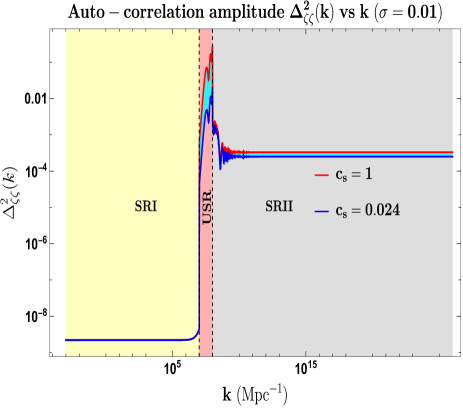
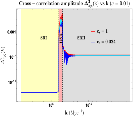
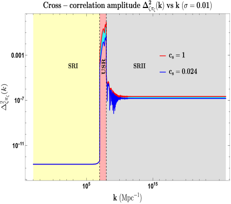
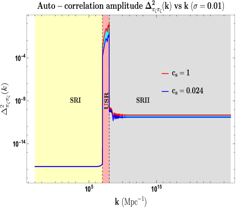
Figure 9: Plot of various power spectrum elements $\Delta^{2}_{fg}$ as function of the wavenumber $k$, where $f,g\;\in\{\zeta,\Pi_{\zeta}\}$. The top-left panel shows the element $\Delta^{2}_{\zeta\zeta}$, the top-right and bottom-left panels show the elements $\Delta^{2}_{\zeta\Pi_{\zeta}}$,$\Delta^{2}_{\Pi_{\zeta}\zeta}$, and the bottom-right panel shows the element $\Delta^{2}_{\Pi_{\zeta}\Pi_{\zeta}}$. The stochastic parameter is fixed to $\sigma=0.01$. The effective sound speed parameter is, $c_{s}=c_{s,*}=\{0.024,1\}$, which is its value fixed at the pivot scale and we plot each correlation for these two values in blue ($c_{s}=0.024$) and red ($c_{s}=1$). All the elements have their behaviour in the three phases, SRI, USR, and SRII, indicated by distinct shading.

In this section, we present with behaviour of the various power spectrum elements as function of the wavenumber across the three phases of interest in our set up, namely SRI, USR, and SRII.

From the fig. (9), we find that the auto-correlation $\Delta^{2}_{\Pi_{\zeta}\Pi_{\zeta}}$, see 9, is the most suppressed in magnitude until slow-roll conditions remain satisfied. This happens during the SRI phase as well as in the SRII phase. In a similar sense, the auto-correlation $\Delta^{2}_{\zeta\zeta}$, see 9, is the most dominant in both the SRI and SRII phases with an amplitude of ${\cal O}(10^{-9})$ in the SRI and ${\cal O}(10^{-3})$ in the SRII phases. The behaviour of all the auto and cross-correlations in the USR duration is more important to note here. All the correlation amplitudes in the USR experience large enhancements to approach magnitudes of order ${\cal O}(10^{-1}-1)$ with the correlation amplitude $\Delta^{2}_{\zeta\zeta}$ being relatively smaller than the other two elements. This fact of the USR have important consequences if we wish to examine the effects from such large enhancements getting carried into the quantum correction calculations. Soon after a sharp exit from the USR occurs at $k=k_{e}$, the amplitude features rapid oscillations till they die out to give a constant magnitude, and these oscillations remain larger in the cross-correlations, see 9 and 9 for $\Delta^{2}_{\zeta\Pi_{\zeta}}$ and $\Delta^{2}_{\Pi_{\zeta}\zeta}$, than in the auto-correlations, $\Delta^{2}_{\zeta\zeta}$ and $\Delta^{2}_{\Pi_{\zeta}\Pi_{\zeta}}$. We put emphasis on the fact that the oscillatory nature of the power spectrum in the USR and after a while into the SRII is a result of the new set of Bogoliubov coefficients, $(\alpha_{2},\beta_{2})$ and $(\alpha_{3},\beta_{3})$ in eqn. (108,109,122,123), which contains complex phase factors after solving for the boundary conditions at each sharp transition $k=k_{s}$ and $k=k_{e}$.

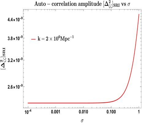
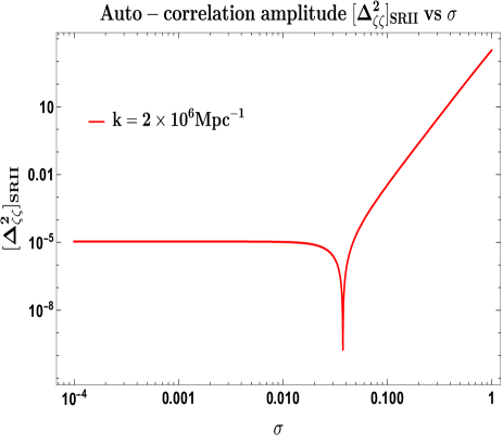
Figure 10: Behaviour of the auto-correlation amplitude $\Delta^{2}_{\zeta\zeta}(k)$ for each phase with respect to change in stochastic parameter $\sigma$. The top row shows for the SRI and USR phase and the bottom for the SRII phase. For $\sigma\in(10^{-4},0.1)$, amplitudes of the correlation in their respective phases remains satisfied and quickly change once $\sigma>0.1$ is considered.

The role played by the effective sound speed, $c_{s}$, is also on display in fig. (9). We show each correlation for two values of $c_{s}=0.024,1$, specifying the lower and upper bounds from observational constraints for causality and unitarity [349]. The red curve corresponds to the case of canonical stochastic single-field inflation, where $c_{s}=c_{s,*}=1$, and here $c_{s,*}$ refers to its value fixed at the pivot scale, see discussions on fig. 3. The value $c_{s,*}=1$ signifies the maximum allowed value, and beyond that, the causality and unitarity constraints get violated. The power spectrum amplitude achieves $\Delta^{2}_{\zeta\zeta}\gtrsim{\cal O}(10^{-2})$ that is more than sufficient to produce PBH. As we decrease $c_{s,*}$ to its lowest value, we get the blue curve where $c_{s,*}=0.024$ and the cyan shaded region in between the two curves represent the possible space of values coming from different $c_{s}$ existing for other non-canonical stochastic single-field models. An important conclusion can be drawn from this is that decreasing sound speed, which keeps the causality and unitarity constraints intact, lowers the amplitude of both the auto-correlations and cross-correlations in the USR phase, thereby keeping the perturbativity assumptions intact. The stochastic parameter value, $\sigma=0.01$, is kept fixed. The lowest amplitude in the USR can reach within $\Delta^{2}_{\zeta\zeta}\sim{\cal O}(10^{-3})$, which is still sufficient from the perspective of PBH production. Also, we highlight here that it is only in the USR where we observe the most significant impact coming from changes in $c_{s}$, while in the two SRI and SRII phases, the changes are minimal, with the least significant being in SRI.

We would now like to underscore the phenomenon of out-of-equilibrium features and first-order phase transitions within the present cosmological set up of stochastic inflation. In the first-order phase transitions, the free energy exhibits a discontinuity in its first derivative, and in the present context, the primordial curvature perturbations and its conjugate momenta play the role of free energies and experience the need to satisfy certain boundary conditions. The Israel junction conditions are the continuity and differentiability requirements imposed during moments of each sharp transition, and this mimics a similar role observed for the phase transitions in statistical physics. As a result, the mode solutions and their conjugate momenta incorporate a different set of Bogoliubov coefficients coming from each subsequent phase transition starting from the SRI phase. The framework of stochastic inflation invites the presence of stochastic effects at the Horizon crossing instant, which comes with a stochastic coarse-graining parameter $\sigma$ and where this parameter facilitates the joining of the different phases near the sharp transitions. Under the influence of stochasticity, at the encounter of each sharp transition, the possible auto-correlations and cross-correlations between the primordial fluctuations become significant and individually bring in out-of-equilibrium effects for the different phases in the vicinity of their Horizon crossing. The net effect is the loss of a precise instance of the quantum to classical phase transition. The stochastic parameter $\sigma$ must always satisfy a magnitude of order $\sigma\ll 1$ to preserve perturbativity in the underlying theoretical framework. The role of $\sigma$ as a coarse-graining factor or a regulator becomes increasingly essential when quantum loop corrections are the subject of interest, and where they can appear in smoothing out the structure of logarithmic IR divergences. The stochastic inflation theory has also received interest in the past to tackle the IR-associated issues in dS space [350, 351, 352, 353, 354, 2, 355, 356, 7]. In the absence of any stochastic features, the dominant contribution comes from the observationally significant auto-correlation $\Delta^{2}_{\zeta\zeta}$ and the other auto-correlation $\Delta^{2}_{\Pi_{\zeta}\Pi_{\zeta}}$ and cross-correlations $\Delta^{2}_{\Pi_{\zeta}\zeta}$ and $\Delta^{2}_{\zeta\Pi_{\zeta}}$ turn out to be highly suppressed.

The fig. 10 show behaviour of the $\Delta^{2}_{\zeta\zeta}$ auto-correlation as a function of the stochastic parameter $\sigma$ for each phase in our set up. Below we append pointwise the interpretation regarding the value of $\sigma$ in each phase:

• In SRI: We notice that for a given wavenumber mode, $k<{\cal O}(10^{7}{\rm Mpc^{-1}})$, the amplitude of the power spectrum in the SRI stays within its magnitude found at the pivot scale, $[\Delta^{2}_{\zeta\zeta}(k)]_{\rm SRI}\sim 2.2\times 10^{-9}$, when we consider the interval of the parameter, $\sigma\in(10^{-4},0.1)$. Beyond the values $\sigma>0.1$, the power spectrum amplitude starts to increase as the contribution coming from the presence of $\sigma$ starts to become increasingly relevant. However, here we must take caution, in that there does not exist a smooth crossover between $\sigma\ll 1$ and $\sigma\sim 1$, as it clearly gives the wrong amplitude for the pivot scale value seen from eqn. (165).

• In USR: We keep fixed a wavenumber $k$ near the transition scale of $k_{s}\sim{\cal O}(10^{7}){\rm Mpc^{-1}}$ as it provides us with the production of large mass PBH, $M_{\rm PBH}\sim{\cal O}(10^{-2}-1\;M_{\odot})$. Having this satisfied, the power spectrum amplitude in the USR reaches $[\Delta^{2}_{\zeta\zeta}(k)]_{\rm USR}\sim{\cal O}(10^{-2})$ which is sufficient to generate PBHs. We notice that for $\sigma\in(10^{-4},0.1)$, the amplitude remains almost a constant value until it rises to reach magnitude of $\sim{\cal O}(10^{-1})$ when $\sigma>0.1$. This interval of the stochastic parameter $\sigma$, prevents amplitude from breaking the perturbativity constraint of reaching $\sim{\cal O}(1)$, and does not greatly enhance the amplitude which can easily lead to overproduction of PBH.

• In SRII: Similar to the two previous phases, in the SRII for a given mode, the respective power spectrum amplitude maintains a value of $[\Delta^{2}_{\zeta\zeta}(k)]_{\rm SRII}\sim{\cal O}(10^{-5})$ till the interval of interest remains $\sigma\in(10^{-4},1)$. The overall amplitude increases at a larger rate afterwards for $\sigma>0.1$, but we again remind of the fact that, within the same setting, a limiting case of $\sigma\sim 1$ cannot be physically interpreted with the behaviour at lower values of $\sigma$. The amplitude quickly breaks perturbativity once $\sigma>0.1$ is considered. We conclude that $\sigma<0.1$ remains a good interval to observe effects of coarse-graining in the power spectrum.

From the above discussions, we find that $\sigma>0.1$ does not lead to meaningful conclusions when comparing with estimates of theoretical and observable importance, such as amplitude of power spectrum at pivot scale, the necessary enhancement for PBH production without overproducing them, and not breaking the perturbativity constraints. On the other hand, any changes coming from $\sigma\ll 1$ remain completely negligible. Hence, we can say that any value of $\sigma<0.1$ suffices to work with and we cannot interpret this scenario with the case of $\sigma>0.1$ together.

A crucial identification can be made directly in reference to the connection between the noise matrix elements and the power spectrum elements as seen before in eqn. (152). As a result of the same formula, in sections VI.1.2, VI.2.2, and VI.3.2, we obtain the noise matrix auto-correlations and cross-correlations corresponding to the respective power spectrum correlations after multiplying with a factor of $(1-\epsilon)$. The value of the slow-roll parameter $\epsilon$ is vanishingly small in the USR while it is still much less than unity in the SRI and SRII, thus indicating that the plots in fig. (9) also represent the behaviour of associated noise auto and cross-correlations. These noise correlations represent effects of the quantum kicks coming from the UV modes after they classicalize in the far super-Horizon (or IR) regions. The $\Sigma_{\zeta\zeta}$ correlation corresponds to most significant of the noise contributions while the correlations involving the conjugate momentum fluctuations, $\Sigma_{\Pi_{\zeta}\zeta}$, $\Sigma_{\zeta\Pi_{\zeta}}$, $\Sigma_{\Pi_{\zeta}\Pi_{\zeta}}$, generate sub-dominant noise amplitudes in the SRI and SRII regime. In the USR, however, all mentioned noise correlations are equally important, implying significant quantum kicks affecting the IR dynamics.

Without including any stochastic features, quantum loop effects have been previously studied by authors in [118, 119, 120, 121]. The existence of a stochastic parameter $\sigma$ serves the purpose of a coarse-graining factor or a regulator in the theory. If one performs the one-loop calculations correctly, then it may happen that in the final result, one can observe the underlying logarithmic IR divergences to be smoothed out more effectively after proper regularization and renormalization techniques than in the calculations done with the absence of such stochastic regulator. We wish to venture towards this goal in the future with great detail. From the perspective of PBHs, their formation faces restrictions in the framework of single-field inflation, where a single-sharp transition occurs. The calculations disallow the formation of any $M_{\rm PBH}\sim{\cal O}(M_{\odot})$ due to solid constraints on the total number of e-folds coming from the necessary procedures of renormalization and a resummation of logarithmic IR divergences at all orders in the loop calculations via the Dynamical Renormalization Group (DRG) analysis [357, 358, 359, 360, 361, 354, 362, 363, 239, 364, 365], $\Delta{\cal N}\sim{\cal O}(20-25)$ (unsuccessful inflation). Some previous attempts, including the presence of multiple sharp transitions (MSTs) [124, 126] and within the framework of single-field Galileon theory with a single sharp transition [121, 122, 123, 127] where the non-renormalization theorem plays the most critical role in tackling the PBH mass constraints, it is shown to avoid this strong restriction and eventually make possible the generation of large solar mass PBHs. The present formalism of stochastic inflation serves as a much better alternative in that with just a single transition, and without bringing in any additional symmetry effects, the stochastic regulator $\sigma$ contains the power to avoid the mentioned restrictions on PBH mass and leads to the formation of $M_{\rm PBH}\sim{\cal O}(M_{\odot})$.

XIV.2 Outcomes of spectral distortions

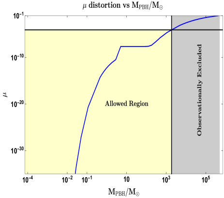
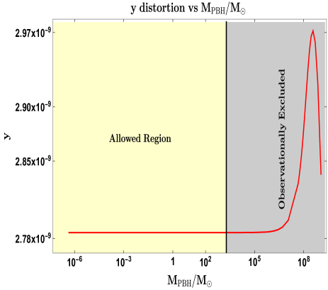
Figure 11: Figure displays the $\mu$-distortion (left-panel), and the y-distortion (right-panel), as function of the PBH mass $M_{\rm PBH}$ (in $M_{\odot}$). The yellow shaded region represents allowed values of the distortion effects after constraints from the COBE/FIRAS observations. The gray shaded regions represents the values disallowed by the same observations.

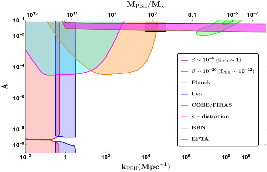
Figure 12: Amplitude of the scalar power spectrum required to achieve non-negligible PBH mass fraction as function of the PBH forming wavenumber $k_{s}$. The background involves constraints on the amplitude coming from the CMB temperature anisotropies (red) [349] at the large scales, Lyman-$\alpha$ forest (blue) [366], COBE/FIRAS (orange) and the y-distortion (cyan) effects [367], BBN (black)[368], and the $1$ and $2\sigma$ contours reported by the pulsar timing array collaboration (green) [178]. The magenta-coloured band, bounded by the brown and purple lines, highlights the region of amplitude where the initial PBH mass fraction from the Press-Schechter formalism lies in the window $\beta\sim{\cal O}(10^{-20}-10^{-8})$.

This section discusses the numerical outcomes for the estimates of the two $\mu$ and $y$ distortion effects. We follow the expressions contained in eqns. (346, 347) to obtain various estimates as function of the PBH mass $M_{\rm PBH}$ formed corresponding to the wavenumber, $k_{\rm PBH}.$

The fig. 11 displays the $\mu$ distortion estimates as function of $M_{\rm PBH}$. Based on the current strongest constraints coming from the COBE/FIRAS observations, the $\mu$ distortion must satisfy, $|\mu|\simeq 9\times 10^{-5}$. The gray shaded region in the plot highlights the excluded mass range as a result of the disallowed $\mu$ values. We notice that the $\mu$ values decrease much rapidly for the masses lower than, $M_{\rm PBH}\lesssim{\cal O}(M\odot)$ and thus make those masses fall in the allowed region. The horizontal line demarcates the above mentioned upper bound on $\mu$ and the black vertical line corresponds to the respective mass value indicating that PBHs with $M_{\rm PBH}\gtrsim 1.8\times 10^{3}\;M_{\odot}$, are equivalently removed from the $\mu$ constraints. The fig. 11 displays the behaviour of the $y$ distortion values as function of the PBH masses. The $y$-distortion does not come out as a significant effect for $M_{\rm PBH}\lesssim{\cal O}(10^{7}M_{\odot})$ after which its behaviour can change in an unpredictable manner. The constraints on this distortion from the COBE/FIRAS observations are $|y|\simeq 1.5\times 10^{-5}$.

To achieve PBH formation requires the scalar power spectrum amplitude to lie within the order of magnitude $A\sim{\cal O}(10^{-2})$. We utilise the same formulas, in eqns. (346, 347), to determine the necessary amplitude such that existing bounds on distortion effects remain satisfied. At the same time, the resulting initial PBH mass fraction should also remain non-negligible and for the same purpose we choose the window of $\beta$ to lie within $\beta\sim{\cal O}(10^{-20}-10^{-8})$.

The figure (12) provides the results for the power spectrum amplitude $A$ as function of the PBH forming wavenumber $k_{s}$. The magenta coloured band highlights the region of initial mass fraction, $\beta\sim{\cal O}(10^{-20}-10^{-8})$, with the interval bounded between purple and brown lines, respectively. The background contains various contours of observational constraint on the amplitude $A$. CMB anisotropy already strictly constraints the primordial power spectrum amplitude at larger scales. We also notice that constraints from the distortion effects, captured by the COBE/FIRAS (in orange) and the regime from y-distortion constraint (in magenta), disfavours PBHs with masses $M_{\rm PBH}\gtrsim 1.8\times 10^{3}M_{\odot}$ upon using the amplitude of $A\sim{\cal O}(10^{-2})$. The earliest studies properly establishing the idea of constraining the primordial power spectrum amplitude by observation of CMB spectral distortions on the larger scales was carried out in [369, 341]. The orange and cyan curves showcase the updated constraints from $\mu-$ and $y-$ type distortions on the power spectrum amplitude, and a detailed analysis on improving these distortion effects constraints and their connections in light of the recently observed stochastic gravitational wave background signal can be found in [367]. The Big Bang Nucleosynthesis (BBN) also limits the amplitude with constraints at the right end of the distortion contour in orange. At scales after BBN but before spectral-distortion era, $k\simeq 10^{4}-10^{5}\;{\rm Mpc^{-1}}$, the energy dissipation of the associated waves ultimately leads to constraints on the primordial power spectrum from overproduction of primordial deuterium and helium estimates. The smaller wavenumbers or larger mass PBH require larger amplitudes, $A\sim{\cal O}(10^{-2}-10^{-1})$, to achieve substantial initial abundance, and that amplitude only tends to increase even faster for $M_{\rm PBH}\gtrsim{\cal O}(10^{11}M_{\odot})$. Going beyond the purple line on top leads to overproduction of PBHs; however, here we remind that the calculations involve the assumption of using an initial Gaussian profile for the curvature perturbation $\zeta$ when examining the distortion estimates with the total power spectrum from eqns. (165, 185, 201).

XIV.3 Outcomes of PDF

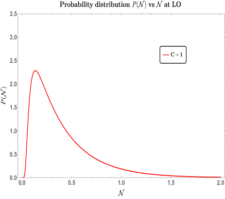
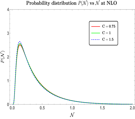
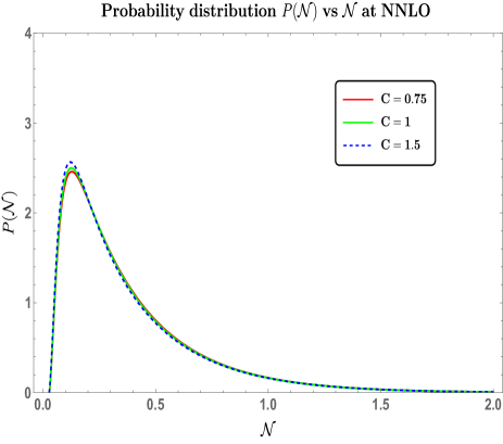
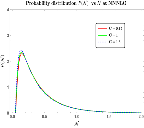
Figure 13: Behaviour of the Probability Distribution Function with changing number of e-folds ${\cal N}$. The top-left panel shows PDF at the leading order (LO) along with different $y$ values. The top-right panel shows the PDF at the next-to-leading order (NLO), the bottom-left panel shows the PDF at the next-to-next-to-leading order (NLO), and the bottom-right panel shows the PDF at the next-to-next-to-next-to-leading order (NLO), all for different values of the characteristic parameter $C=\{0.75,1,1.5\}$ in red, green, blue, respectively.

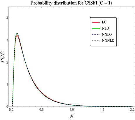
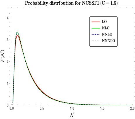
Figure 14: Plot shows PDF as a function of the stochastic variable ${\cal N}$ including all order of the perturbative expansion up to NNNLO. The left-panel considers the case of canonical stochastic single-field inflation $(C=1)$ superposed with all the distinct PDF from the perturbative expansion and, similarly, the right-panel considers the case of non-canonical single-field inflation $(C=1.5)$.

In this section, we study the outcomes of our PDF calculations upto the order NNNLO in the diffusion-dominated regime. The expressions for the PDF at the NNLO and NNNLO have not been discussed explicitly but here we provide with their graphical representations and discuss their features. The initial phase space variables $(x,y)$ are defined previously in eqn. (233), as being related to the coarse-grained curvature perturbation and its conjugate momentum variable.

We begin with the analysis at the leading order (LO). Earlier eqn. (262) did not saw any involvement of the characteristic parameter $C$ in the residues, as well as the poles. From eqn. (257), it is clear that in order to explicitly observe $C$ requires the existence of higher-order poles, at least where $m=1$. The fig. 13 shows the distribution from eqn. (262), plotted against the stochastic e-folding number, ${\cal N}$, for a fixed $C=1$. Since this is at the leading order in $y$ expansion, no change in the features for changing $y$ is observed. The remaining parameters are fixed here to have $x=1$ and $\tilde{\mu}=0.9$. Going to the next order in the expansion, we now have two sets of poles that combine to give the full PDF at NLO, displayed in the fig.(13). The analytic expression is also available from eqn. (297). Notice the difference in curves associated with different scenarios of non-canonical single-field inflation, characterized by a finite and changing $C$. The relative difference is not significant enough to render the EFT description undesirable. We have chosen here to keep $C$ close to $1$, as seen from the red and dotted blue curves. This time, the amplitude has risen compared to the LO case, with the difference being in the first decimal place. Here $y=0.15$ is fixed while $x=1$ and $\tilde{\mu}=0.9$ remain the same. In this regime of $y$ values, most of the PDF gets well approximated by the leading terms in the series expansion of eqn. (287) as the rest decay very quickly. Further in the bottom-left fig. 13 we have the PDF at the NNLO. The analytic expression for this PDF is not made explicit before but we can see from the distribution that its behaviour remains almost similar to the previous PDFs with small relative changes at the maximum when different values of $C$ are considered. The peak amplitude is also close to the PDF at NLO with differences now pushed to the second decimal place. The parameter set, $x=1$, $y=0.15$, and $\tilde{\mu}=1$, is kept fixed. In the bottom-right panel of fig. (13), we finally consider the distribution at NNNLO. The peak amplitude shows clear changes for various $C$ values in the allowed range for a valid EFT formulation and the amplitude change relative to NNLO now occurs at the first decimal place and lowers the estimate. This also signals preserving the perturbativity argument in the analysis after keeping fixed the same set of values for the other parameters, $x=1$, $y=0.15$, and $\tilde{\mu}=1$.

In the diffusion-dominated regime, we conclude that the distribution functions at subsequent orders maintain the perturbativity conditions satisfactorily. The observed changes for various EFT descriptions are characterized by $C$ value of interest only near the peak amplitude regions, and the size of the differences does not drastically change the overall features of the PDF. At all orders shown in fig.(13), the left and right tails follow similar trends, and only slight changes are visible near the peak amplitude.

The figure 14 displays behaviour of all the distribution functions superimposed, that captures various higher-order corrections in the diffusion-dominated regime in the small $y$ limit, keeping $y=0.073$, $x=1$, and $\tilde{\mu}=0.76$ fixed. The reason for the choice of these values of the parameters is related to the resulting PBH abundance features that we expect in the upcoming sections and will be justified shortly. After we superimpose the PDFs, we notice almost negligible changes in the values for the PDF. This time, the expansion variable $y$ is also kept much lower than the analysis in fig. (13), and this is reflected in the fact that relative differences in the amplitude are pushed further to the second and third decimal places. The $C=1$ in fig. 14 represents canonical stochastic single-field inflation scenario while the case $C=1.5$ in fig. 14 represents the non-canonical stochastic single-field inflation scenario. The peak amplitudes remain close to each other thus keeping perturbativity intact and the the tail features are also similar across different orders. The distributions for the non-canonical scenario also remain relatively similar except for small changes in the peak amplitude, at the second decimal places. Also, the behaviour of the fall near ${\cal N}\sim 0.5$ changes slightly between the LO and the rest of subsequent orders combined. The total combination of dominant contribution from the leading reside $r^{(0)}_{n,i}$, where $i$ specifies the order of expansion, and the poles $\Lambda_{n}^{(0)}$ quickly give the similar dominant features in the PDF at all orders in the fig. 14.

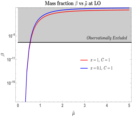
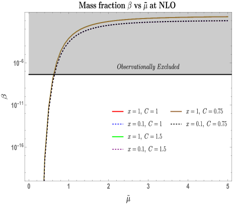
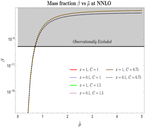
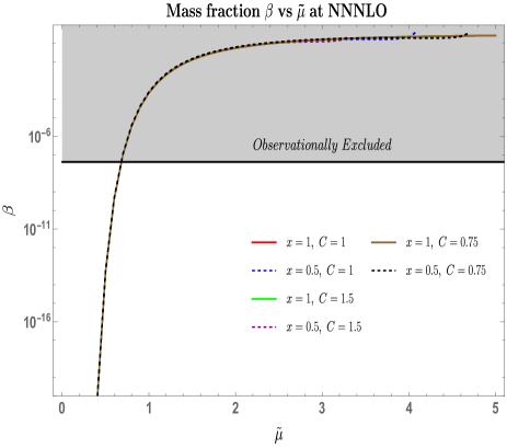
Figure 15: Mass fraction $\beta$ against variation in $\tilde{\mu}$. The mass fraction is extremely sensitive to $\mu$ values close to or less than $1$ and equally less sensitive to changes in $x$. The top-left panel displays behaviour of $\beta$ for PDF at LO, $P_{\Gamma}^{\rm LO}({\cal N})$ and does not incorporate a variable $C$. The top-right panel displays behaviour of $\beta$ for PDF at NLO, $P_{\Gamma}^{\rm NLO}({\cal N})$, the bottom-left panel displays behaviour of $\beta$ for PDF at NNLO, $P_{\Gamma}^{\rm NNLO}({\cal N})$, and the bottom-right panel displays behaviour of $\beta$ for PDF at NNNLO, $P_{\Gamma}^{\rm NNNLO}({\cal N})$. Multiple cases with values of $C\in\{0.75,1,1.5\}$ are shown. The gray shaded region highlights the values of $\beta\gtrsim{\cal O}(10^{-8})$ excluded by current observations for heavy mass PBH, in the range $10^{16}$g to $10^{50}$g (or $M_{\rm PBH}\sim{\cal O}(10^{-17}-10^{16})M_{\odot}$).

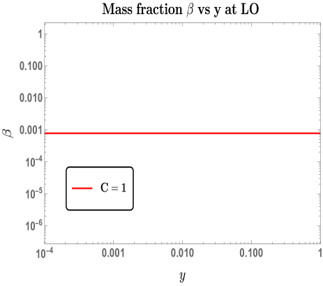
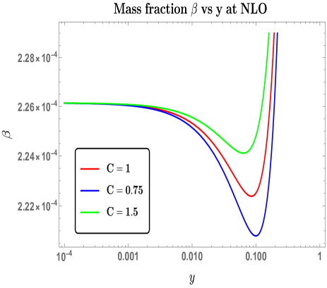
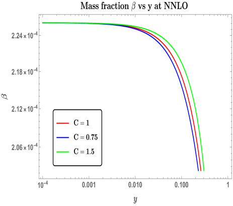
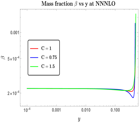
Figure 16: Mass fraction $\beta$ against variation in $y$. The top-left panel displays behaviour of $\beta$ at LO with changing $y$ and does not incorporate variable $C\neq 1$. The top-right panel displays behaviour of $\beta$ at NLO with $y$, the bottom-left panel displays behaviour of $\beta$ at NNLO with changing $y$, and the bottom-right panel displays behaviour of $\beta$ at NNNLO with changing $y$. Multiple cases with values of $C=1$ (red), $C=0.75$ (blue), and $C=1.5$ (green) are shown and $x=1$ with $\tilde{\mu}=1$ and $\zeta_{\rm th}\sim{\cal O}(1)$ are kept fixed.

XIV.4 Outcomes from PBH mass fraction $\beta$

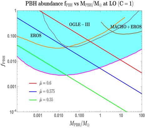
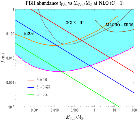
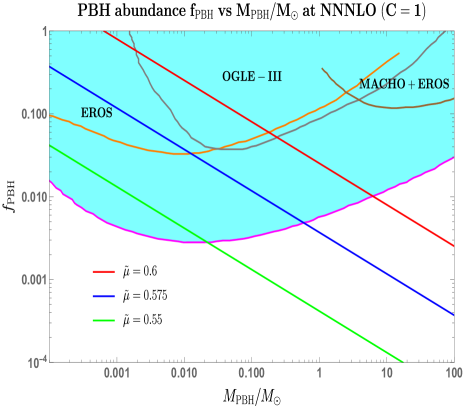
Figure 17: PBH abundance $f_{\rm PBH}$ as a function of the mass (in $M_{\odot}$). The fixed values of different parameters are $x=1$, $y=0.06$, and $C=1$. Each plot features different values of $\mu\in\{0.55,0.575,0.6\}$. The cyan-coloured region highlights the recently obtained $95\%$ upper limits on PBH abundance from microlensing events. The magenta boundary marks the strict limits on $f_{\rm PBH}$ [370] and also includes limits from other dark matter surveys: EROS (orange) [371], OGLE-III (gray) [372], MACHO+EROS (brown) [373].

In this section we analyze the results for the PBH mass fraction and abundance based on the analytical treatment of the distribution functions for the diffusion-dominated regime. The fig. (15) features behaviour of the PBH mass fraction for changing values of $\tilde{\mu}$. Here, $\beta$ experiences steep change in its value for $\tilde{\mu}\leqslant 1$ and after $\tilde{\mu}$ becomes greater than $1$, the mass fraction quickly saturates to values close to but less than $1$. Changes in $x$ have little impact on $\beta$ and the effects only become distinguishable once $\tilde{\mu}\geqslant 1$. The left-panel shows $\beta$ when PDF at leading order is considered. It displays the scenario of canonical stochastic single-field inflation. The right-panel focuses on $\beta$ from the PDF at next-to-leading order. The effects of various $C$ is not significant enough to distinguish but we notice that $\beta$ at NLO, for $\tilde{\mu}\geqslant 1$, changes by a lesser amount as $x$ is decreased compared to the $\beta$ at LO. Also, the PDF at NLO predicts less mass fraction compared to the PDF at LO for the same $\tilde{\mu}$ value. Hence, mass fraction is observed to decrease by at least one order in magnitude for $\tilde{\mu}\leqslant 1$.

Focusing on the next order in the perturbative expansion, we get the mass fraction behaviour from the PDF at NNLO in the bottom-left fig. 15. The mass fraction suffers a further decrease of an order of magnitude for $\tilde{\mu}\leqslant 1$. The rate of decrease in $\beta$ has also improved for smaller $\tilde{\mu}$ values. This will have significant implications when we consider the resulting PBH abundance from the mass fraction. Similar to the previous case at NLO, the effects coming from the characteristic parameter $C$ in the mass fraction are not significant enough to distinguish properly. Lastly, some interesting changes happen with the PDF at NNNLO and its derived $\beta$ behaviour. From fig. 15 for $\beta$ at NNNLO, we notice that for $x=0.5$, a positive magnitude of $\beta$ lasts up to a certain value of $\tilde{\mu}>1$ after which the numerical values return negative results. Thus, $x$ cannot be decreased to very less values as doing so would only push $\beta$ to negative values faster and for values of $\mu\sim 1$. The relative change after decreasing $x$ from $x=1$ has also almost vanished. The effects of the characteristic parameter $C$ is more interesting to notice here. Increasing $C$ beyond $C=1$ along with $x<1$, results with the corresponding $\beta$ going negative for lower values of $\tilde{\mu}$ as compared to lowering $C$ than $C=1$, in which case the $\beta$ extends to larger $\tilde{\mu}$ until it again drops to negative values. No such issue arises when $x\gtrsim 1$ is considered.

In the fig. 16, we explore the behaviour of the mass fraction $\beta$, at each order in the perturbative expansion, with changing values of $y$ or the coarse-grained conjugate momentum variable as defined before in eqn. (233). Since this behaviour is studied using the features of diffusion-dominated regime, see section X, it follows that the limit of $y\ll 1$ would provide for much suitable interval from where PBH mass fraction can get estimated accurately, including higher-order corrections of NNNLO analysis. The leading order (LO) scenario is an expansion independent of $y$, hence, any change with $y$ in the top-left panel 16 would not give any useful insights into the mass fraction behaviour. Going to the NLO scenario, here we get additional terms linear in $y$ to our PDF and as a consequence we observe, from the top-right panel, fig. 16, small changes to $\beta$. In terms of different $C$ values, the relative separation becomes larger as we set $y>0.01$. The mass fraction then changes quickly by at least an order of magnitude, increasing till we reach $y\sim 1$. The effect of sub-dominant corrections changes as we consider the NNLO case, fig. 16. Here, the mass fraction $\beta$ continues to move further lower in magnitude as $y>0.01$ is considered. Mass fraction for the lower values, $C<1$, fall early as compared to the higher values, $C\geqslant 1$. At last we consider the correction up to NNNLO to $\beta$ and analyse their effects from fig. 16. This time, the mass fraction stays the same for a large interval of $y<0.1$. Even while taking multiple $C$ into account, the relative difference only becomes significant if we choose to have $y>0.5$. The case of canonical stochastic single-field $(C=1)$ does not show much differences and only changes sharply by an order of magnitude when we reach $y\sim 1$. The mass fraction converges to have similar behaviour for different $C$ values in the $(y\ll 1)$ and $y\sim 1$ limits.

We conclude by saying that the choice of interval $y\sim{\cal O}(0.01)$ agrees well after comparison between each higher-order correction to the mass fraction $\beta$. For $y\geqslant 0.1$, the behaviour can change non-trivially and depending on the order of expansion considered.

XIV.5 Outcomes from PBH abundance $f_{PBH}$

In this section we discuss the observed outcomes for the PBH abundance as function of the PBH mass after the magnitude of curvature perturbations exceed a threshold value of $\zeta_{\rm th}\sim{\cal O}(1).$

The fig. (17) features in it the abundance of a spectrum of PBH masses ranging from $M_{\rm PBH}\sim{\cal O}(10^{-4}M_{\odot})$ to $M_{\rm PBH}\sim{\cal O}(10^{2}M_{\odot})$. The plots shows that the abundance is extremely sensitive to the values of $\tilde{\mu}$ for a fixed $x=1$, $y=0.06$, $C=1$ and keeping $\zeta_{\rm th}\sim{\cal O}(1)$ satisfied throughout. With the distribution function at different orders we observe from the various sub-figures, 17, 17, 17, 17, the scenario of a large enough mass range that can achieve sizeable PBH abundance as a result. The higher we go in the perturbation expansion, their influence on the abundance remains the same with relatively small deviations throughout the mass range being explored. We include the results obtained from different micorlensing surveys on the fraction of total dark matter distributed in form of PBHs. The cyan coloured region with solid magenta line marks the region constrained from the data of Optical Gravitational Lensing Experiment (OGLE) in their $20$ years run which comprises of the OGLE-III $(2001-2009)$ and OGLE-IV $(2010-2020)$ runs. For more details on the observation setup and proper data generation analysis consider studies in [374, 370]. From the strict constraints, we infer that large $M_{\rm PBH}\sim{\cal O}(1-100)M_{\odot}$ can compose at most $10\%$ fraction of the total dark matter. The sensitivity to the corrections in PDF at each order can be seen more clearly from the plot in fig. 18. The leading order (LO) contribution predicts a larger magnitude of abundance relative to the next-to-leading order (NLO) corrections coming from the associated PDF, and the subsequent corrections do not bring much noticeable changes.

The threshold curvature perturbation $\zeta_{\rm th}$ is another important parameter to manipulate. Changes in its value show high sensitivity to the possible $\tilde{\mu}$ values, with the larger $\tilde{\mu}\geqslant 0.5$ being more sensitive to $\zeta_{\rm th}$ resulting in a sizeable abundance than compared to lower values of $\tilde{\mu}\leqslant 0.5$. The right-panel, fig. 18, features the effect of changing $\zeta_{\rm th}$ for a fixed $\tilde{\mu}$ and fixed PBH mass, $M_{\rm PBH}\sim{\cal O}(10^{-3}M_{\odot})$, including corrections from all cases in the perturbative analysis of the PDF. Effects of threshold change is found to be independent of the order of correction considered in the PDF expansion and likewise in the PBH abundance which follows, as a result, similar decreasing trend upon increasing the threshold. From the slope of 18, we can also interpret that changing $\tilde{\mu}$ affects the abundance for different masses in the same manner for a given $C$ value. We conclude with the fact that additional perturbative corrections to the PDF bring in almost negligible changes into the abundance estimates for a large spectrum of PBH masses and the quantity $f_{\rm PBH}$ is highly sensitive to changes in $\tilde{\mu}$ which affects all PBH masses equally for a certain threshold $\zeta_{\rm th}$.

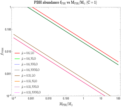
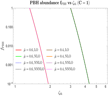
Figure 18: left-panel displays PBH abundance $f_{\rm PBH}$ as function of the mass (in $M_{\odot}$) including all orders of the perturbative expansion. right-panel shows $f_{\rm PBH}$ as function of the threshold $\zeta_{\rm th}$ including all order of the perturbative expansion. The figures are for a fixed set of $\tilde{\mu}\in\{0.55,0.6\}$ and $C=1$.

XV Comparison with previous works

A broad collection of previous and latest works has focused on applying the stochastic inflation formalism and its newer version using the language of standard, classical $\delta N$-formalism. In this section, we perform a comparative study between the conclusions of previous works using the stochastic-$\delta N$ formalism with focus on their connection with primordial black holes and highlight differences in the perturbative analysis of the probability distribution driving the stochastic e-folding ${\cal N}$.

The stochastic-$\delta N$ formalism was developed initially in refs.[228, 229, 230]. These works paved the way by introducing a new algorithm for calculating the correlation functions of the curvature perturbation after utilizing the $\delta N$-formalism technique and solving for multiple realizations of the Langevin equation. Some of the works [53, 159, 38, 232, 231] have also focused on applying stochastic-$\delta N$ techniques to the scenario where quantum diffusion effects play a significant role for a certain period during inflation. Such effects also generate sizeable primordial curvature fluctuations, which initiate PBH formation post-inflation. A consequence of these stochastic effects is the fluctuation in the e-folds and the stochastic-$\delta N$ formalism helps to extract the statistics of the curvature perturbation in language of the e-folding statistics. PBH formation events are rare, and difference in the tail of the curvature perturbation distribution heavily impacts their abundance. In the paper [159], they have developed methods for and conducted a thorough analysis on the implications of higher-order corrections on PBH mass fraction, with showing methods to obtain explicit moments of the variable ${\cal N}$, analysed there till the next-to-leading order (NLO). Our work builds upon the previously laid understandings and extends it to visualize the effects of considering even higher-order correction till the next-to-next-to-next-to-leading order (NNNLO) and develop the whole analysis in a field-independent picture. The result is an effective field theory (EFT) description of stochastic single field inflation, where the EFT effects come with a new parameter dubbed the characteristic parameter $C$, see eqn. (238). The range of $C$ is taken to be close to unity considering the behaviour of slow-roll parameters in different regimes of interest, including the ultra-slow roll during inflation. For the canonical stochastic single-field scenario, or when we set $C=1$, our results for the distribution function and PBH mass fraction analysis agree with previous discussions elaborated in [159]. From here, we venture further into a detailed higher-order PDF analysis both in the drift and diffusion-dominated regime, keeping account of the changes coming from the $C$ parameter throughout. For the drift regime, building on the foundations from [159], the derived PDF supplies corrections to various non-Gaussianity parameters at each order of its analysis. These corrections are computed including $C$ dependence, as opposed to previous works with canonical single-field models, and we estimate behaviour of the PDF shape around its mean via measures such as skewness and kurtosis for each correction order. In the diffusion-dominated regime, our analysis, inspired primarily from [38, 159], casts previous attempts into the EFT language and again looks into higher-order corrections, focusing on the tail features. The diffusion regime follows a sophisticated analysis of carefully considering, in the present context, the allowed correction in line with the order of expansion and its variable. Our extended explicit analysis of the PDF till NNNLO finds the perturbative approximations remaining completely consistent. Similar to the above-mentioned attempts, we also study implications of the diffusion regime PDF analysis on to the PBH mass fraction and abundance with a $C$ dependent feature. Another crucial aspect of our work, which appears differently, is a detailed examination of the stochastic effects in the possible auto and cross-correlated power spectrum amplitudes and their inherent connection with the respective noise matrix elements. The analytic study focuses on a general quasi de Sitter spacetime and arbitrary initial quantum vacuum state conditions. The impact of stochasticity, specifically the regulatory features of the coarse-graining parameter $\sigma$, and the importance of each correlation in the present setup is stressed thoroughly.

XVI Conclusion

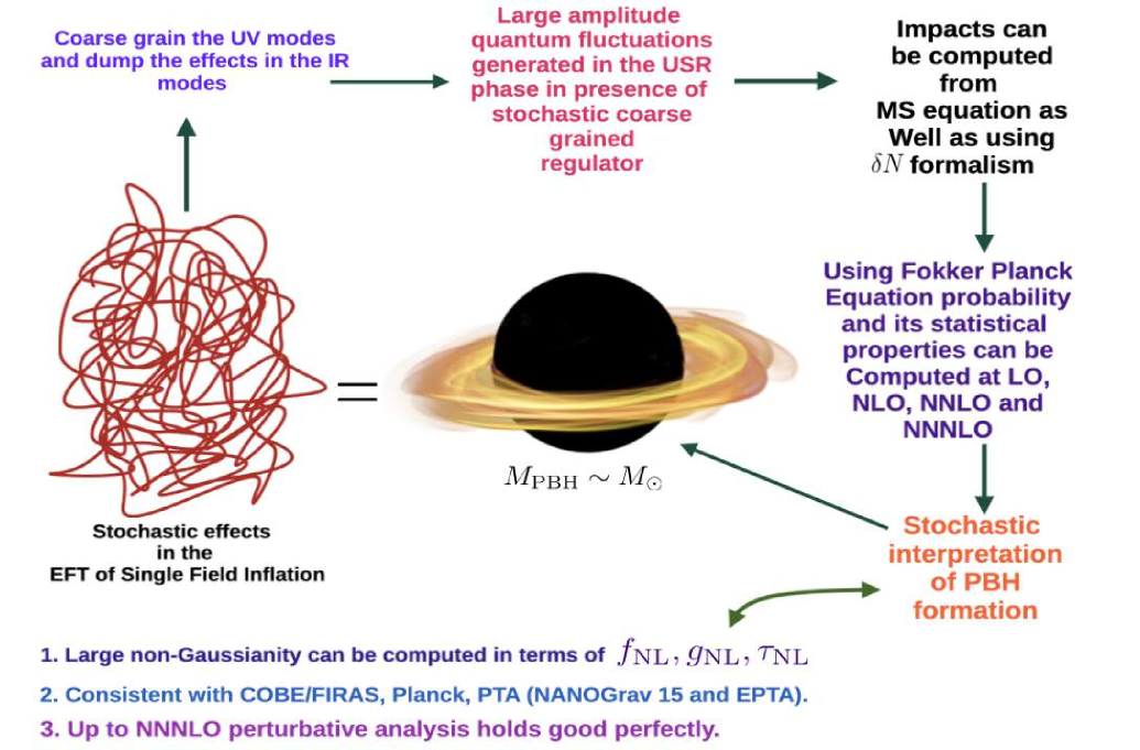
Figure 19: Illustrative diagram describing the main features and results from this work. The results from this work include computation of various non-Gaussianity parameters, $f_{\rm NL},g_{\rm NL},\tau_{\rm NL}$, following perturbative corrections coming from each order in the diffusion-dominated regime.

The focus of this work is threefold. We attempt to develop an Effective Field Theory (EFT) understanding of stochastic single-field inflation. In parallel with the stochastic-$\delta N$ formalism, we perform a more precise analysis of the non-Gaussianity features in the drift-dominated regime and the tail features responsible for PBH formation when in the diffusion-dominated regime. Finally, we study the tree-level scalar power spectrum, both auto-correlated and cross-correlated amplitudes, in the framework of stochastic formalism.

We build the effective theory description of the long-wavelength part of the curvature perturbations, following closely the works of [164, 43], and solve for the Hamilton’s equations of motion for the coarse-grained variables. We give the modified, EFT version of the Langevin equations, which govern the evolution of the coarse-grained variables. Following earlier developments, we provide the essential modifications in the Fokker-Planck equation driving the probability distribution of the stochastic duration variable ${\cal N}$. The consequence of working in the EFT language comes with a new characteristic parameter, $C$, in the Fokker-Planck equation, whose values describe a class of models, either canonical $(C=1)$ or non-canonical $(C\neq 1)$, in stochastic single-field inflation. The parameter $C$ is shown to be determined by a combination of slow-roll parameters, which ultimately carry the EFT picture into the remainder of our analysis concerning non-Gaussianity and PBH formation. Before continuing with this detailed analysis, we outline a comparative study focusing on the merits of the stochastic-$\delta N$ formalism and how this new integrated version of the two different frameworks will help us in our later computations in the drift and diffusion-dominated regimes.

In the drift-dominated regime, the analysis carried out up to the next-to-next-to-next-to-leading order (NNNLO) shows $C$ dependent corrections coming into each order version of the non-Gaussianity parameters, $f_{\rm NL},g_{\rm NL},\tau_{\rm NL}$, and equivalently into the related statistical moments of the stochastic e-folds ${\cal N}$. The probability distribution function (PDF) of the e-folds ${\cal N}$ is given at each order of the analysis, and the effects of the parameter $C$ on the PDF shape at each order via measures such as skewness and kurtosis are also provided. In the diffusion-dominated regime, a similar perturbative analysis up to NNNLO is given for the distribution function. Though explicit expressions become greatly cumbersome beyond next-to-leading order (NLO), numerical results are possible to design. The perturbative expansion is shown through figure 14 to hold perfectly for this regime. The analytic expressions for the mean number of e-folds are given at each order, which later appears to contribute to the PBH mass fraction using stochastic-$\delta N$ formalism.

The implications of corrections up to NNNLO, in the diffusion-dominated scenario, on the PBH formation shows an order of decrease in the magnitude of mass fraction $\beta$ when the other parameter $\tilde{\mu}$, containing the tree-level scalar power spectrum, remains of $\tilde{\mu}\gtrsim 1$. However, for $\tilde{\mu}<1$, the mass fraction suffers a steep decrease, a change of least two orders in magnitude, as lower values are taken for $\tilde{\mu}$. The above shows that taking into account higher-order corrections can reduce the mass fraction to favourable estimates in a controllable manner, see figure 15 for details. Changes from $C$ are not discernible from the numerical outcomes at each order as they remain very small. The current-day PBH abundance outcomes also reflect the similar effect of taking higher-order corrections into account. The abundance reduces equally for a range of PBH masses, $M_{\rm PBH}\sim{\cal O}(10^{-4}-10^{2}M_{\odot})$, and further corrections from NNLO and NNNLO do not bring in visible changes; see figure 18 for the same. We also provide explicit expressions for the tree-level scalar power spectrum after including stochastic effects for each possible auto and cross-correlation amplitude. Here, the stochastic parameter $\sigma$, where $\sigma\ll 1$, is shown to play a crucial role by acting as a regulator in the presence of large quantum fluctuations and promoting controlled behaviour of the correlations at the transition junctions from SRI to USR and USR to SRII, which we outline. The impact of different effective sound speed parameters, $c_{s}$, is also treated for each correlation amplitude. We find that $c_{s}=1$ manages to provide a correlation amplitude of, $\Delta^{2}_{\zeta\zeta}\sim{\cal O}(10^{-2})$, in the USR that also enables PBH production, and upon lowering $c_{s}$ within the constraint coming from experimental analysis, $0.024\leqslant c_{s}<1$, reduces the amplitude to, $\Delta^{2}_{\zeta\zeta}\sim{\cal O}(10^{-3})$. The above allows us to infer that by keeping the causality and unitarity constraints satisfied, with the value of $c_{s}$ in the mentioned interval, the correlation amplitude always tends to decrease, which also implies preserving the underlying perturbativity assumptions. As an aside, we discuss some important features of the $\sigma$ parameter when quantum loop corrections get treated as a genuine concern from each of the mentioned possible power spectrum correlations. On the observational side, we also explore the spectral distortion effects, which require the use of the tree-level scalar power spectrum. As a result of the strong constraints on the power spectrum amplitude from such effects, the case of PBH mass with $M_{\rm PBH}\gtrsim 1.8\times 10^{3}M_{\odot}$ remains excluded.

Figure 19 pictorially summarizes the results of this work and lists out the key findings from observational features involved with PBHs and non-Gaussianity parameters. We have a plan to carry forward our analysis by incorporating the quantum loop effects in the presence of stochasticity in the soft de Sitter EFT framework using both Schwinger Keldysh (in-in) and stochastic-$\delta{\cal N}$ formalism. In this extended version of the work, we have a further plan to study the issues related to renormalization, DRG resummation, and its connection to the stochastic-$\delta{\cal N}$ formalism.

References

- [1] A. A. Starobinsky, “STOCHASTIC DE SITTER (INFLATIONARY) STAGE IN THE EARLY UNIVERSE,” Lect. Notes Phys. 246 (1986) 107–126.
- [2] V. Gorbenko and L. Senatore, “ in dS,” arXiv:1911.00022 [hep-th].
- [3] T. Cohen, D. Green, A. Premkumar, and A. Ridgway, “Stochastic Inflation at NNLO,” JHEP 09 (2021) 159, arXiv:2106.09728 [hep-th].
- [4] T. Cohen, D. Green, and A. Premkumar, “Large deviations in the early Universe,” Phys. Rev. D 107 no. 8, (2023) 083501, arXiv:2212.02535 [hep-th].
- [5] D. Green, “EFT for de Sitter Space,” arXiv:2210.05820 [hep-th].
- [6] T. Cohen, D. Green, and A. Premkumar, “A tail of eternal inflation,” SciPost Phys. 14 no. 5, (2023) 109, arXiv:2111.09332 [hep-th].
- [7] T. Cohen and D. Green, “Soft de Sitter Effective Theory,” JHEP 12 (2020) 041, arXiv:2007.03693 [hep-th].
- [8] Y. B. Zel’dovich and I. D. Novikov, “The Hypothesis of Cores Retarded during Expansion and the Hot Cosmological Model,” Soviet Astron. AJ (Engl. Transl. ), 10 (1967) 602.
- [9] S. W. Hawking, “Black hole explosions,” Nature 248 (1974) 30–31.
- [10] B. J. Carr and S. W. Hawking, “Black holes in the early Universe,” Mon. Not. Roy. Astron. Soc. 168 (1974) 399–415.
- [11] B. J. Carr, “The Primordial black hole mass spectrum,” Astrophys. J. 201 (1975) 1–19.
- [12] G. F. Chapline, “Cosmological effects of primordial black holes,” Nature 253 no. 5489, (1975) 251–252.
- [13] B. J. Carr and J. E. Lidsey, “Primordial black holes and generalized constraints on chaotic inflation,” Phys. Rev. D 48 (1993) 543–553.
- [14] S. Choudhury and S. Pal, “Fourth level MSSM inflation from new flat directions,” JCAP 04 (2012) 018, arXiv:1111.3441 [hep-ph].
- [15] J. Yokoyama, “Chaotic new inflation and formation of primordial black holes,” Phys. Rev. D 58 (1998) 083510, arXiv:astro-ph/9802357.
- [16] M. Kawasaki and T. Yanagida, “Primordial black hole formation in supergravity,” Phys. Rev. D 59 (1999) 043512, arXiv:hep-ph/9807544.
- [17] S. G. Rubin, A. S. Sakharov, and M. Y. Khlopov, “The Formation of primary galactic nuclei during phase transitions in the early universe,” J. Exp. Theor. Phys. 91 (2001) 921–929, arXiv:hep-ph/0106187.
- [18] M. Y. Khlopov, S. G. Rubin, and A. S. Sakharov, “Strong primordial inhomogeneities and galaxy formation,” arXiv:astro-ph/0202505.
- [19] M. Y. Khlopov, S. G. Rubin, and A. S. Sakharov, “Primordial structure of massive black hole clusters,” Astropart. Phys. 23 (2005) 265, arXiv:astro-ph/0401532.
- [20] R. Saito, J. Yokoyama, and R. Nagata, “Single-field inflation, anomalous enhancement of superhorizon fluctuations, and non-Gaussianity in primordial black hole formation,” JCAP 06 (2008) 024, arXiv:0804.3470 [astro-ph].
- [21] M. Y. Khlopov, “Primordial Black Holes,” Res. Astron. Astrophys. 10 (2010) 495–528, arXiv:0801.0116 [astro-ph].
- [22] B. J. Carr, K. Kohri, Y. Sendouda, and J. Yokoyama, “New cosmological constraints on primordial black holes,” Phys. Rev. D 81 (2010) 104019, arXiv:0912.5297 [astro-ph.CO].
- [23] D. H. Lyth, “Primordial black hole formation and hybrid inflation,” arXiv:1107.1681 [astro-ph.CO].
- [24] M. Drees and E. Erfani, “Running Spectral Index and Formation of Primordial Black Hole in Single Field Inflation Models,” JCAP 01 (2012) 035, arXiv:1110.6052 [astro-ph.CO].
- [25] M. Drees and E. Erfani, “Running-Mass Inflation Model and Primordial Black Holes,” JCAP 04 (2011) 005, arXiv:1102.2340 [hep-ph].
- [26] J. M. Ezquiaga, J. Garcia-Bellido, and E. Ruiz Morales, “Primordial Black Hole production in Critical Higgs Inflation,” Phys. Lett. B 776 (2018) 345–349, arXiv:1705.04861 [astro-ph.CO].
- [27] K. Kannike, L. Marzola, M. Raidal, and H. Veermäe, “Single Field Double Inflation and Primordial Black Holes,” JCAP 09 (2017) 020, arXiv:1705.06225 [astro-ph.CO].
- [28] M. P. Hertzberg and M. Yamada, “Primordial Black Holes from Polynomial Potentials in Single Field Inflation,” Phys. Rev. D 97 no. 8, (2018) 083509, arXiv:1712.09750 [astro-ph.CO].
- [29] S. Pi, Y.-l. Zhang, Q.-G. Huang, and M. Sasaki, “Scalaron from -gravity as a heavy field,” JCAP 05 (2018) 042, arXiv:1712.09896 [astro-ph.CO].
- [30] T.-J. Gao and Z.-K. Guo, “Primordial Black Hole Production in Inflationary Models of Supergravity with a Single Chiral Superfield,” Phys. Rev. D 98 no. 6, (2018) 063526, arXiv:1806.09320 [hep-ph].
- [31] I. Dalianis, A. Kehagias, and G. Tringas, “Primordial black holes from -attractors,” JCAP 01 (2019) 037, arXiv:1805.09483 [astro-ph.CO].
- [32] M. Cicoli, V. A. Diaz, and F. G. Pedro, “Primordial Black Holes from String Inflation,” JCAP 06 (2018) 034, arXiv:1803.02837 [hep-th].
- [33] O. Özsoy, S. Parameswaran, G. Tasinato, and I. Zavala, “Mechanisms for Primordial Black Hole Production in String Theory,” JCAP 07 (2018) 005, arXiv:1803.07626 [hep-th].
- [34] C. T. Byrnes, P. S. Cole, and S. P. Patil, “Steepest growth of the power spectrum and primordial black holes,” JCAP 06 (2019) 028, arXiv:1811.11158 [astro-ph.CO].
- [35] G. Ballesteros, J. Beltran Jimenez, and M. Pieroni, “Black hole formation from a general quadratic action for inflationary primordial fluctuations,” JCAP 06 (2019) 016, arXiv:1811.03065 [astro-ph.CO].
- [36] K. M. Belotsky, V. I. Dokuchaev, Y. N. Eroshenko, E. A. Esipova, M. Y. Khlopov, L. A. Khromykh, A. A. Kirillov, V. V. Nikulin, S. G. Rubin, and I. V. Svadkovsky, “Clusters of primordial black holes,” Eur. Phys. J. C 79 no. 3, (2019) 246, arXiv:1807.06590 [astro-ph.CO].
- [37] J. Martin, T. Papanikolaou, and V. Vennin, “Primordial black holes from the preheating instability in single-field inflation,” JCAP 01 (2020) 024, arXiv:1907.04236 [astro-ph.CO].
- [38] J. M. Ezquiaga, J. García-Bellido, and V. Vennin, “The exponential tail of inflationary fluctuations: consequences for primordial black holes,” JCAP 03 (2020) 029, arXiv:1912.05399 [astro-ph.CO].
- [39] H. Motohashi, S. Mukohyama, and M. Oliosi, “Constant Roll and Primordial Black Holes,” JCAP 03 (2020) 002, arXiv:1910.13235 [gr-qc].
- [40] C. Fu, P. Wu, and H. Yu, “Primordial Black Holes from Inflation with Nonminimal Derivative Coupling,” Phys. Rev. D 100 no. 6, (2019) 063532, arXiv:1907.05042 [astro-ph.CO].
- [41] A. Ashoorioon, A. Rostami, and J. T. Firouzjaee, “EFT compatible PBHs: effective spawning of the seeds for primordial black holes during inflation,” JHEP 07 (2021) 087, arXiv:1912.13326 [astro-ph.CO].
- [42] P. Auclair and V. Vennin, “Primordial black holes from metric preheating: mass fraction in the excursion-set approach,” JCAP 02 (2021) 038, arXiv:2011.05633 [astro-ph.CO].
- [43] V. Vennin, Stochastic inflation and primordial black holes. PhD thesis, U. Paris-Saclay, 6, 2020. arXiv:2009.08715 [astro-ph.CO].
- [44] D. V. Nanopoulos, V. C. Spanos, and I. D. Stamou, “Primordial Black Holes from No-Scale Supergravity,” Phys. Rev. D 102 no. 8, (2020) 083536, arXiv:2008.01457 [astro-ph.CO].
- [45] K. Inomata, E. McDonough, and W. Hu, “Primordial black holes arise when the inflaton falls,” Phys. Rev. D 104 no. 12, (2021) 123553, arXiv:2104.03972 [astro-ph.CO].
- [46] I. D. Stamou, “Mechanisms of producing primordial black holes by breaking the symmetry,” Phys. Rev. D 103 no. 8, (2021) 083512, arXiv:2104.08654 [hep-ph].
- [47] K.-W. Ng and Y.-P. Wu, “Constant-rate inflation: primordial black holes from conformal weight transitions,” JHEP 11 (2021) 076, arXiv:2102.05620 [astro-ph.CO].
- [48] Q. Wang, Y.-C. Liu, B.-Y. Su, and N. Li, “Primordial black holes from the perturbations in the inflaton potential in peak theory,” Phys. Rev. D 104 no. 8, (2021) 083546, arXiv:2111.10028 [astro-ph.CO].
- [49] S. Kawai and J. Kim, “Primordial black holes from Gauss-Bonnet-corrected single field inflation,” Phys. Rev. D 104 no. 8, (2021) 083545, arXiv:2108.01340 [astro-ph.CO].
- [50] M. Solbi and K. Karami, “Primordial black holes formation in the inflationary model with field-dependent kinetic term for quartic and natural potentials,” Eur. Phys. J. C 81 no. 10, (2021) 884, arXiv:2106.02863 [astro-ph.CO].
- [51] G. Ballesteros, S. Céspedes, and L. Santoni, “Large power spectrum and primordial black holes in the effective theory of inflation,” JHEP 01 (2022) 074, arXiv:2109.00567 [hep-th].
- [52] G. Rigopoulos and A. Wilkins, “Inflation is always semi-classical: diffusion domination overproduces Primordial Black Holes,” JCAP 12 no. 12, (2021) 027, arXiv:2107.05317 [astro-ph.CO].
- [53] C. Animali and V. Vennin, “Primordial black holes from stochastic tunnelling,” JCAP 02 (2023) 043, arXiv:2210.03812 [astro-ph.CO].
- [54] D. Frolovsky, S. V. Ketov, and S. Saburov, “Formation of primordial black holes after Starobinsky inflation,” Mod. Phys. Lett. A 37 no. 21, (2022) 2250135, arXiv:2205.00603 [astro-ph.CO].
- [55] A. Escrivà, F. Kuhnel, and Y. Tada, “Primordial Black Holes,” arXiv:2211.05767 [astro-ph.CO].
- [56] O. Özsoy and G. Tasinato, “Inflation and Primordial Black Holes,” arXiv:2301.03600 [astro-ph.CO].
- [57] P. Ivanov, P. Naselsky, and I. Novikov, “Inflation and primordial black holes as dark matter,” Phys. Rev. D 50 (1994) 7173–7178.
- [58] N. Afshordi, P. McDonald, and D. N. Spergel, “Primordial black holes as dark matter: The Power spectrum and evaporation of early structures,” Astrophys. J. Lett. 594 (2003) L71–L74, arXiv:astro-ph/0302035.
- [59] P. H. Frampton, M. Kawasaki, F. Takahashi, and T. T. Yanagida, “Primordial Black Holes as All Dark Matter,” JCAP 04 (2010) 023, arXiv:1001.2308 [hep-ph].
- [60] B. Carr, F. Kuhnel, and M. Sandstad, “Primordial Black Holes as Dark Matter,” Phys. Rev. D 94 no. 8, (2016) 083504, arXiv:1607.06077 [astro-ph.CO].
- [61] M. Kawasaki, A. Kusenko, Y. Tada, and T. T. Yanagida, “Primordial black holes as dark matter in supergravity inflation models,” Phys. Rev. D 94 no. 8, (2016) 083523, arXiv:1606.07631 [astro-ph.CO].
- [62] K. Inomata, M. Kawasaki, K. Mukaida, Y. Tada, and T. T. Yanagida, “Inflationary Primordial Black Holes as All Dark Matter,” Phys. Rev. D 96 no. 4, (2017) 043504, arXiv:1701.02544 [astro-ph.CO].
- [63] J. R. Espinosa, D. Racco, and A. Riotto, “Cosmological Signature of the Standard Model Higgs Vacuum Instability: Primordial Black Holes as Dark Matter,” Phys. Rev. Lett. 120 no. 12, (2018) 121301, arXiv:1710.11196 [hep-ph].
- [64] G. Ballesteros and M. Taoso, “Primordial black hole dark matter from single field inflation,” Phys. Rev. D 97 no. 2, (2018) 023501, arXiv:1709.05565 [hep-ph].
- [65] M. Sasaki, T. Suyama, T. Tanaka, and S. Yokoyama, “Primordial black holes—perspectives in gravitational wave astronomy,” Class. Quant. Grav. 35 no. 6, (2018) 063001, arXiv:1801.05235 [astro-ph.CO].
- [66] G. Ballesteros, J. Rey, and F. Rompineve, “Detuning primordial black hole dark matter with early matter domination and axion monodromy,” JCAP 06 (2020) 014, arXiv:1912.01638 [astro-ph.CO].
- [67] I. Dalianis and G. Tringas, “Primordial black hole remnants as dark matter produced in thermal, matter, and runaway-quintessence postinflationary scenarios,” Phys. Rev. D 100 no. 8, (2019) 083512, arXiv:1905.01741 [astro-ph.CO].
- [68] D. Y. Cheong, S. M. Lee, and S. C. Park, “Primordial black holes in Higgs- inflation as the whole of dark matter,” JCAP 01 (2021) 032, arXiv:1912.12032 [hep-ph].
- [69] A. M. Green and B. J. Kavanagh, “Primordial Black Holes as a dark matter candidate,” J. Phys. G 48 no. 4, (2021) 043001, arXiv:2007.10722 [astro-ph.CO].
- [70] B. Carr and F. Kuhnel, “Primordial Black Holes as Dark Matter: Recent Developments,” Ann. Rev. Nucl. Part. Sci. 70 (2020) 355–394, arXiv:2006.02838 [astro-ph.CO].
- [71] G. Ballesteros, J. Rey, M. Taoso, and A. Urbano, “Primordial black holes as dark matter and gravitational waves from single-field polynomial inflation,” JCAP 07 (2020) 025, arXiv:2001.08220 [astro-ph.CO].
- [72] B. Carr, K. Kohri, Y. Sendouda, and J. Yokoyama, “Constraints on primordial black holes,” Rept. Prog. Phys. 84 no. 11, (2021) 116902, arXiv:2002.12778 [astro-ph.CO].
- [73] O. Özsoy and Z. Lalak, “Primordial black holes as dark matter and gravitational waves from bumpy axion inflation,” JCAP 01 (2021) 040, arXiv:2008.07549 [astro-ph.CO].
- [74] D. Baumann, P. J. Steinhardt, K. Takahashi, and K. Ichiki, “Gravitational Wave Spectrum Induced by Primordial Scalar Perturbations,” Phys. Rev. D 76 (2007) 084019, arXiv:hep-th/0703290.
- [75] R. Saito and J. Yokoyama, “Gravitational wave background as a probe of the primordial black hole abundance,” Phys. Rev. Lett. 102 (2009) 161101, arXiv:0812.4339 [astro-ph]. [Erratum: Phys.Rev.Lett. 107, 069901 (2011)].
- [76] R. Saito and J. Yokoyama, “Gravitational-Wave Constraints on the Abundance of Primordial Black Holes,” Prog. Theor. Phys. 123 (2010) 867–886, arXiv:0912.5317 [astro-ph.CO]. [Erratum: Prog.Theor.Phys. 126, 351–352 (2011)].
- [77] S. Choudhury and A. Mazumdar, “Primordial blackholes and gravitational waves for an inflection-point model of inflation,” Phys. Lett. B 733 (2014) 270–275, arXiv:1307.5119 [astro-ph.CO].
- [78] M. Sasaki, T. Suyama, T. Tanaka, and S. Yokoyama, “Primordial Black Hole Scenario for the Gravitational-Wave Event GW150914,” Phys. Rev. Lett. 117 no. 6, (2016) 061101, arXiv:1603.08338 [astro-ph.CO]. [Erratum: Phys.Rev.Lett. 121, 059901 (2018)].
- [79] M. Raidal, V. Vaskonen, and H. Veermäe, “Gravitational Waves from Primordial Black Hole Mergers,” JCAP 09 (2017) 037, arXiv:1707.01480 [astro-ph.CO].
- [80] T. Papanikolaou, V. Vennin, and D. Langlois, “Gravitational waves from a universe filled with primordial black holes,” JCAP 03 (2021) 053, arXiv:2010.11573 [astro-ph.CO].
- [81] Y. Ali-Haïmoud, E. D. Kovetz, and M. Kamionkowski, “Merger rate of primordial black-hole binaries,” Phys. Rev. D 96 no. 12, (2017) 123523, arXiv:1709.06576 [astro-ph.CO].
- [82] H. Di and Y. Gong, “Primordial black holes and second order gravitational waves from ultra-slow-roll inflation,” JCAP 07 (2018) 007, arXiv:1707.09578 [astro-ph.CO].
- [83] M. Raidal, C. Spethmann, V. Vaskonen, and H. Veermäe, “Formation and Evolution of Primordial Black Hole Binaries in the Early Universe,” JCAP 02 (2019) 018, arXiv:1812.01930 [astro-ph.CO].
- [84] S.-L. Cheng, W. Lee, and K.-W. Ng, “Primordial black holes and associated gravitational waves in axion monodromy inflation,” JCAP 07 (2018) 001, arXiv:1801.09050 [astro-ph.CO].
- [85] V. Vaskonen and H. Veermäe, “Lower bound on the primordial black hole merger rate,” Phys. Rev. D 101 no. 4, (2020) 043015, arXiv:1908.09752 [astro-ph.CO].
- [86] M. Drees and Y. Xu, “Overshooting, Critical Higgs Inflation and Second Order Gravitational Wave Signatures,” Eur. Phys. J. C 81 no. 2, (2021) 182, arXiv:1905.13581 [hep-ph].
- [87] A. Hall, A. D. Gow, and C. T. Byrnes, “Bayesian analysis of LIGO-Virgo mergers: Primordial vs. astrophysical black hole populations,” Phys. Rev. D 102 (2020) 123524, arXiv:2008.13704 [astro-ph.CO].
- [88] A. Ashoorioon, A. Rostami, and J. T. Firouzjaee, “Examining the end of inflation with primordial black holes mass distribution and gravitational waves,” Phys. Rev. D 103 (2021) 123512, arXiv:2012.02817 [astro-ph.CO].
- [89] L. Wu, Y. Gong, and T. Li, “Primordial black holes and secondary gravitational waves from string inspired general no-scale supergravity,” Phys. Rev. D 104 no. 12, (2021) 123544, arXiv:2105.07694 [gr-qc].
- [90] R. Kimura, T. Suyama, M. Yamaguchi, and Y.-L. Zhang, “Reconstruction of Primordial Power Spectrum of curvature perturbation from the merger rate of Primordial Black Hole Binaries,” JCAP 04 (2021) 031, arXiv:2102.05280 [astro-ph.CO].
- [91] M. Solbi and K. Karami, “Primordial black holes and induced gravitational waves in -inflation,” JCAP 08 (2021) 056, arXiv:2102.05651 [astro-ph.CO].
- [92] Z. Teimoori, K. Rezazadeh, M. A. Rasheed, and K. Karami, “Mechanism of primordial black holes production and secondary gravitational waves in -attractor Galileon inflationary scenario,” arXiv:2107.07620 [astro-ph.CO].
- [93] M. Cicoli, F. G. Pedro, and N. Pedron, “Secondary GWs and PBHs in string inflation: formation and detectability,” JCAP 08 no. 08, (2022) 030, arXiv:2203.00021 [hep-th].
- [94] A. Ashoorioon, K. Rezazadeh, and A. Rostami, “NANOGrav signal from the end of inflation and the LIGO mass and heavier primordial black holes,” Phys. Lett. B 835 (2022) 137542, arXiv:2202.01131 [astro-ph.CO].
- [95] T. Papanikolaou, “Gravitational waves induced from primordial black hole fluctuations: the effect of an extended mass function,” JCAP 10 (2022) 089, arXiv:2207.11041 [astro-ph.CO].
- [96] T. Papanikolaou, “Primordial black holes in loop quantum cosmology: the effect on the threshold,” Class. Quant. Grav. 40 no. 13, (2023) 134001, arXiv:2301.11439 [gr-qc].
- [97] X. Wang, Y.-l. Zhang, R. Kimura, and M. Yamaguchi, “Reconstruction of Power Spectrum of Primordial Curvature Perturbations on small scales from Primordial Black Hole Binaries scenario of LIGO/VIRGO detection,” arXiv:2209.12911 [astro-ph.CO].
- [98] R. Zheng, J. Shi, and T. Qiu, “On primordial black holes and secondary gravitational waves generated from inflation with solo/multi-bumpy potential ,” Chin. Phys. C 46 no. 4, (2022) 045103, arXiv:2106.04303 [astro-ph.CO].
- [99] A. R. Brown, “Hyperbolic Inflation,” Phys. Rev. Lett. 121 no. 25, (2018) 251601, arXiv:1705.03023 [hep-th].
- [100] G. A. Palma, S. Sypsas, and C. Zenteno, “Seeding primordial black holes in multifield inflation,” Phys. Rev. Lett. 125 no. 12, (2020) 121301, arXiv:2004.06106 [astro-ph.CO].
- [101] S. R. Geller, W. Qin, E. McDonough, and D. I. Kaiser, “Primordial black holes from multifield inflation with nonminimal couplings,” Phys. Rev. D 106 no. 6, (2022) 063535, arXiv:2205.04471 [hep-th].
- [102] M. Braglia, A. Linde, R. Kallosh, and F. Finelli, “Hybrid -attractors, primordial black holes and gravitational wave backgrounds,” arXiv:2211.14262 [astro-ph.CO].
- [103] D. Frolovsky and S. V. Ketov, “Fitting power spectrum of scalar perturbations for primordial black hole production during inflation,” arXiv:2302.06153 [astro-ph.CO].
- [104] Y. Aldabergenov and S. V. Ketov, “Primordial black holes from Volkov-Akulov-Starobinsky supergravity,” arXiv:2301.12750 [hep-th].
- [105] S. Aoki, R. Ishikawa, and S. V. Ketov, “Pole inflation and primordial black holes formation in Starobinsky-like supergravity,” Class. Quant. Grav. 40 no. 6, (2023) 065002, arXiv:2210.10348 [hep-th].
- [106] D. Frolovsky, S. V. Ketov, and S. Saburov, “E-models of inflation and primordial black holes,” Front. in Phys. 10 (2022) 1005333, arXiv:2207.11878 [astro-ph.CO].
- [107] Y. Aldabergenov, A. Addazi, and S. V. Ketov, “Inflation, SUSY breaking, and primordial black holes in modified supergravity coupled to chiral matter,” Eur. Phys. J. C 82 no. 8, (2022) 681, arXiv:2206.02601 [astro-ph.CO].
- [108] R. Ishikawa and S. V. Ketov, “Exploring the parameter space of modified supergravity for double inflation and primordial black hole formation,” Class. Quant. Grav. 39 no. 1, (2022) 015016, arXiv:2108.04408 [astro-ph.CO].
- [109] A. Gundhi, S. V. Ketov, and C. F. Steinwachs, “Primordial black hole dark matter in dilaton-extended two-field Starobinsky inflation,” Phys. Rev. D 103 no. 8, (2021) 083518, arXiv:2011.05999 [hep-th].
- [110] Y. Aldabergenov, A. Addazi, and S. V. Ketov, “Primordial black holes from modified supergravity,” Eur. Phys. J. C 80 no. 10, (2020) 917, arXiv:2006.16641 [hep-th].
- [111] R.-g. Cai, S. Pi, and M. Sasaki, “Gravitational Waves Induced by non-Gaussian Scalar Perturbations,” Phys. Rev. Lett. 122 no. 20, (2019) 201101, arXiv:1810.11000 [astro-ph.CO].
- [112] S.-L. Cheng, D.-S. Lee, and K.-W. Ng, “Power spectrum of primordial perturbations during ultra-slow-roll inflation with back reaction effects,” Phys. Lett. B 827 (2022) 136956, arXiv:2106.09275 [astro-ph.CO].
- [113] S. Balaji, J. Silk, and Y.-P. Wu, “Induced gravitational waves from the cosmic coincidence,” JCAP 06 no. 06, (2022) 008, arXiv:2202.00700 [astro-ph.CO].
- [114] W. Qin, S. R. Geller, S. Balaji, E. McDonough, and D. I. Kaiser, “Planck Constraints and Gravitational Wave Forecasts for Primordial Black Hole Dark Matter Seeded by Multifield Inflation,” arXiv:2303.02168 [astro-ph.CO].
- [115] A. Riotto, “The Primordial Black Hole Formation from Single-Field Inflation is Not Ruled Out,” arXiv:2301.00599 [astro-ph.CO].
- [116] A. Riotto, “The Primordial Black Hole Formation from Single-Field Inflation is Still Not Ruled Out,” arXiv:2303.01727 [astro-ph.CO].
- [117] T. Papanikolaou, A. Lymperis, S. Lola, and E. N. Saridakis, “Primordial black holes and gravitational waves from non-canonical inflation,” JCAP 03 (2023) 003, arXiv:2211.14900 [astro-ph.CO].
- [118] S. Choudhury, M. R. Gangopadhyay, and M. Sami, “No-go for the formation of heavy mass Primordial Black Holes in Single Field Inflation,” arXiv:2301.10000 [astro-ph.CO].
- [119] S. Choudhury, S. Panda, and M. Sami, “PBH formation in EFT of single field inflation with sharp transition,” Phys. Lett. B 845 (2023) 138123, arXiv:2302.05655 [astro-ph.CO].
- [120] S. Choudhury, S. Panda, and M. Sami, “Quantum loop effects on the power spectrum and constraints on primordial black holes,” JCAP 11 (2023) 066, arXiv:2303.06066 [astro-ph.CO].
- [121] S. Choudhury, S. Panda, and M. Sami, “Galileon inflation evades the no-go for PBH formation in the single-field framework,” JCAP 08 (2023) 078, arXiv:2304.04065 [astro-ph.CO].
- [122] S. Choudhury, A. Karde, S. Panda, and M. Sami, “Primordial non-Gaussianity from ultra slow-roll Galileon inflation,” JCAP 01 (2024) 012, arXiv:2306.12334 [astro-ph.CO].
- [123] S. Choudhury, A. Karde, S. Panda, and M. Sami, “Scalar induced gravity waves from ultra slow-roll Galileon inflation,” arXiv:2308.09273 [astro-ph.CO].
- [124] G. Bhattacharya, S. Choudhury, K. Dey, S. Ghosh, A. Karde, and N. S. Mishra, “Evading no-go for PBH formation and production of SIGWs using Multiple Sharp Transitions in EFT of single field inflation,” arXiv:2309.00973 [astro-ph.CO].
- [125] S. Choudhury, K. Dey, A. Karde, S. Panda, and M. Sami, “Primordial non-Gaussianity as a saviour for PBH overproduction in SIGWs generated by Pulsar Timing Arrays for Galileon inflation,” arXiv:2310.11034 [astro-ph.CO].
- [126] S. Choudhury, K. Dey, and A. Karde, “Untangling PBH overproduction in -SIGWs generated by Pulsar Timing Arrays for MST-EFT of single field inflation,” arXiv:2311.15065 [astro-ph.CO].
- [127] S. Choudhury, A. Karde, S. Panda, and M. Sami, “Realisation of the ultra-slow roll phase in Galileon inflation and PBH overproduction,” arXiv:2401.10925 [astro-ph.CO].
- [128] T. Harada, C.-M. Yoo, and K. Kohri, “Threshold of primordial black hole formation,” Phys. Rev. D 88 no. 8, (2013) 084051, arXiv:1309.4201 [astro-ph.CO]. [Erratum: Phys.Rev.D 89, 029903 (2014)].
- [129] T. Harada, C.-M. Yoo, K. Kohri, and K.-I. Nakao, “Spins of primordial black holes formed in the matter-dominated phase of the Universe,” Phys. Rev. D 96 no. 8, (2017) 083517, arXiv:1707.03595 [gr-qc]. [Erratum: Phys.Rev.D 99, 069904 (2019)].
- [130] T. Kokubu, K. Kyutoku, K. Kohri, and T. Harada, “Effect of Inhomogeneity on Primordial Black Hole Formation in the Matter Dominated Era,” Phys. Rev. D 98 no. 12, (2018) 123024, arXiv:1810.03490 [astro-ph.CO].
- [131] B.-M. Gu, F.-W. Shu, and K. Yang, “Inflation with shallow dip and primordial black holes,” arXiv:2307.00510 [astro-ph.CO].
- [132] S. Saburov and S. V. Ketov, “Improved Model of Primordial Black Hole Formation after Starobinsky Inflation,” Universe 9 no. 7, (2023) 323, arXiv:2306.06597 [gr-qc].
- [133] I. D. Stamou, “Exploring critical overdensity thresholds in inflationary models of primordial black holes formation,” Phys. Rev. D 108 no. 6, (2023) 063515, arXiv:2306.02758 [astro-ph.CO].
- [134] S. Libanore, M. Liguori, and A. Raccanelli, “Signatures of primordial black holes in gravitational wave clustering,” JCAP 08 (2023) 055, arXiv:2306.03087 [astro-ph.CO].
- [135] A. Friedlander, N. Song, and A. C. Vincent, “Dark matter from higher-dimensional primordial black holes,” Phys. Rev. D 108 no. 4, (2023) 043523, arXiv:2306.01520 [hep-ph].
- [136] C. Chen, A. Ghoshal, Z. Lalak, Y. Luo, and A. Naskar, “Growth of curvature perturbations for PBH formation & detectable GWs in non-minimal curvaton scenario revisited,” JCAP 08 (2023) 041, arXiv:2305.12325 [astro-ph.CO].
- [137] Y. Cai, M. Zhu, and Y.-S. Piao, “Primordial black holes from null energy condition violation during inflation,” arXiv:2305.10933 [gr-qc].
- [138] A. Karam, N. Koivunen, E. Tomberg, A. Racioppi, and H. Veermäe, “Primordial black holes and inflation from double-well potentials,” JCAP 09 (2023) 002, arXiv:2305.09630 [astro-ph.CO].
- [139] L. Iacconi and D. J. Mulryne, “Multi-field inflation with large scalar fluctuations: non-Gaussianity and perturbativity,” JCAP 09 (2023) 033, arXiv:2304.14260 [astro-ph.CO].
- [140] T. C. Gehrman, B. Shams Es Haghi, K. Sinha, and T. Xu, “The primordial black holes that disappeared: connections to dark matter and MHz-GHz gravitational Waves,” JCAP 10 (2023) 001, arXiv:2304.09194 [hep-ph].
- [141] L. E. Padilla, J. C. Hidalgo, and G. German, “Constraining inflationary potentials with inflaton PBHs,” Phys. Rev. D 108 no. 6, (2023) 063511, arXiv:2303.16428 [astro-ph.CO].
- [142] K.-P. Xie, “Pinning down the primordial black hole formation mechanism with gamma-rays and gravitational waves,” JCAP 06 (2023) 008, arXiv:2301.02352 [astro-ph.CO].
- [143] D.-S. Meng, C. Yuan, and Q.-G. Huang, “Primordial black holes generated by the non-minimal spectator field,” Sci. China Phys. Mech. Astron. 66 no. 8, (2023) 280411, arXiv:2212.03577 [astro-ph.CO].
- [144] T. Qiu, W. Wang, and R. Zheng, “Generation of primordial black holes from an inflation model with modified dispersion relation,” Phys. Rev. D 107 no. 8, (2023) 083018, arXiv:2212.03403 [astro-ph.CO].
- [145] B. Mu, G. Cheng, J. Liu, and Z.-K. Guo, “Constraints on ultraslow-roll inflation from the third LIGO-Virgo observing run,” Phys. Rev. D 107 no. 4, (2023) 043528, arXiv:2211.05386 [astro-ph.CO].
- [146] C. Fu and S.-J. Wang, “Primordial black holes and induced gravitational waves from double-pole inflation,” JCAP 06 (2023) 012, arXiv:2211.03523 [astro-ph.CO].
- [147] M. W. Davies, L. Iacconi, and D. J. Mulryne, “Numerical 1-loop correction from a potential yielding ultra-slow-roll dynamics,” arXiv:2312.05694 [astro-ph.CO].
- [148] H. Firouzjahi and A. Riotto, “Primordial Black Holes and Loops in Single-Field Inflation,” arXiv:2304.07801 [astro-ph.CO].
- [149] H. Firouzjahi, “One-loop Corrections in Power Spectrum in Single Field Inflation,” arXiv:2303.12025 [astro-ph.CO].
- [150] L. Iacconi, D. Mulryne, and D. Seery, “Loop corrections in the separate universe picture,” arXiv:2312.12424 [astro-ph.CO].
- [151] J. H. P. Jackson, H. Assadullahi, A. D. Gow, K. Koyama, V. Vennin, and D. Wands, “The separate-universe approach and sudden transitions during inflation,” arXiv:2311.03281 [astro-ph.CO].
- [152] A. Riotto and J. Silk, “The Future of Primordial Black Holes: Open Questions and Roadmap,” arXiv:2403.02907 [astro-ph.CO].
- [153] V. Vennin and D. Wands, “Quantum diffusion and large primordial perturbations from inflation,” arXiv:2402.12672 [astro-ph.CO].
- [154] C. Animali and V. Vennin, “Clustering of primordial black holes from quantum diffusion during inflation,” arXiv:2402.08642 [astro-ph.CO].
- [155] LISA Cosmology Working Group Collaboration, E. Bagui et al., “Primordial black holes and their gravitational-wave signatures,” arXiv:2310.19857 [astro-ph.CO].
- [156] J. M. Ezquiaga, J. García-Bellido, and V. Vennin, “Could ”El Gordo” be hinting at primordial quantum diffusion?,” arXiv:2207.06317 [astro-ph.CO].
- [157] J. H. P. Jackson, H. Assadullahi, K. Koyama, V. Vennin, and D. Wands, “Numerical simulations of stochastic inflation using importance sampling,” JCAP 10 (2022) 067, arXiv:2206.11234 [astro-ph.CO].
- [158] Y. Tada and V. Vennin, “Statistics of coarse-grained cosmological fields in stochastic inflation,” JCAP 02 no. 02, (2022) 021, arXiv:2111.15280 [astro-ph.CO].
- [159] C. Pattison, V. Vennin, D. Wands, and H. Assadullahi, “Ultra-slow-roll inflation with quantum diffusion,” JCAP 04 (2021) 080, arXiv:2101.05741 [astro-ph.CO].
- [160] K. Ando and V. Vennin, “Power spectrum in stochastic inflation,” JCAP 04 (2021) 057, arXiv:2012.02031 [astro-ph.CO].
- [161] C. Pattison, V. Vennin, H. Assadullahi, and D. Wands, “Stochastic inflation beyond slow roll,” JCAP 07 (2019) 031, arXiv:1905.06300 [astro-ph.CO].
- [162] M. Noorbala, V. Vennin, H. Assadullahi, H. Firouzjahi, and D. Wands, “Tunneling in Stochastic Inflation,” JCAP 09 (2018) 032, arXiv:1806.09634 [hep-th].
- [163] C. Pattison, V. Vennin, H. Assadullahi, and D. Wands, “Quantum diffusion during inflation and primordial black holes,” JCAP 10 (2017) 046, arXiv:1707.00537 [hep-th].
- [164] J. Grain and V. Vennin, “Stochastic inflation in phase space: Is slow roll a stochastic attractor?,” JCAP 05 (2017) 045, arXiv:1703.00447 [gr-qc].
- [165] R. J. Hardwick, V. Vennin, C. T. Byrnes, J. Torrado, and D. Wands, “The stochastic spectator,” JCAP 10 (2017) 018, arXiv:1701.06473 [astro-ph.CO].
- [166] NANOGrav Collaboration, G. Agazie et al., “The NANOGrav 15 yr Data Set: Evidence for a Gravitational-wave Background,” Astrophys. J. Lett. 951 no. 1, (2023) L8, arXiv:2306.16213 [astro-ph.HE].
- [167] NANOGrav Collaboration, G. Agazie et al., “The NANOGrav 15 yr Data Set: Observations and Timing of 68 Millisecond Pulsars,” Astrophys. J. Lett. 951 no. 1, (2023) L9, arXiv:2306.16217 [astro-ph.HE].
- [168] NANOGrav Collaboration, G. Agazie et al., “The NANOGrav 15 yr Data Set: Detector Characterization and Noise Budget,” Astrophys. J. Lett. 951 no. 1, (2023) L10, arXiv:2306.16218 [astro-ph.HE].
- [169] NANOGrav Collaboration, A. Afzal et al., “The NANOGrav 15 yr Data Set: Search for Signals from New Physics,” Astrophys. J. Lett. 951 no. 1, (2023) L11, arXiv:2306.16219 [astro-ph.HE].
- [170] NANOGrav Collaboration, G. Agazie et al., “The NANOGrav 15 yr Data Set: Constraints on Supermassive Black Hole Binaries from the Gravitational-wave Background,” Astrophys. J. Lett. 952 no. 2, (2023) L37, arXiv:2306.16220 [astro-ph.HE].
- [171] NANOGrav Collaboration, G. Agazie et al., “The NANOGrav 15-year Data Set: Search for Anisotropy in the Gravitational-Wave Background,” arXiv:2306.16221 [astro-ph.HE].
- [172] NANOGrav Collaboration, G. Agazie et al., “The NANOGrav 15 yr Data Set: Bayesian Limits on Gravitational Waves from Individual Supermassive Black Hole Binaries,” Astrophys. J. Lett. 951 no. 2, (2023) L50, arXiv:2306.16222 [astro-ph.HE].
- [173] NANOGrav Collaboration, A. D. Johnson et al., “The NANOGrav 15-year Gravitational-Wave Background Analysis Pipeline,” arXiv:2306.16223 [astro-ph.HE].
- [174] EPTA Collaboration, J. Antoniadis et al., “The second data release from the European Pulsar Timing Array III. Search for gravitational wave signals,” arXiv:2306.16214 [astro-ph.HE].
- [175] EPTA Collaboration, J. Antoniadis et al., “The second data release from the European Pulsar Timing Array I. The dataset and timing analysis,” arXiv:2306.16224 [astro-ph.HE].
- [176] EPTA Collaboration, J. Antoniadis et al., “The second data release from the European Pulsar Timing Array II. Customised pulsar noise models for spatially correlated gravitational waves,” arXiv:2306.16225 [astro-ph.HE].
- [177] EPTA Collaboration, J. Antoniadis et al., “The second data release from the European Pulsar Timing Array IV. Search for continuous gravitational wave signals,” arXiv:2306.16226 [astro-ph.HE].
- [178] EPTA Collaboration, J. Antoniadis et al., “The second data release from the European Pulsar Timing Array: V. Implications for massive black holes, dark matter and the early Universe,” arXiv:2306.16227 [astro-ph.CO].
- [179] EPTA Collaboration, C. Smarra et al., “The second data release from the European Pulsar Timing Array: VI. Challenging the ultralight dark matter paradigm,” arXiv:2306.16228 [astro-ph.HE].
- [180] D. J. Reardon et al., “Search for an Isotropic Gravitational-wave Background with the Parkes Pulsar Timing Array,” Astrophys. J. Lett. 951 no. 1, (2023) L6, arXiv:2306.16215 [astro-ph.HE].
- [181] D. J. Reardon et al., “The Gravitational-wave Background Null Hypothesis: Characterizing Noise in Millisecond Pulsar Arrival Times with the Parkes Pulsar Timing Array,” Astrophys. J. Lett. 951 no. 1, (2023) L7, arXiv:2306.16229 [astro-ph.HE].
- [182] A. Zic et al., “The Parkes Pulsar Timing Array Third Data Release,” arXiv:2306.16230 [astro-ph.HE].
- [183] H. Xu et al., “Searching for the Nano-Hertz Stochastic Gravitational Wave Background with the Chinese Pulsar Timing Array Data Release I,” Res. Astron. Astrophys. 23 no. 7, (2023) 075024, arXiv:2306.16216 [astro-ph.HE].
- [184] K. Inomata, K. Kohri, and T. Terada, “The Detected Stochastic Gravitational Waves and Subsolar-Mass Primordial Black Holes,” arXiv:2306.17834 [astro-ph.CO].
- [185] G. Franciolini, A. Iovino, Junior., V. Vaskonen, and H. Veermae, “Recent Gravitational Wave Observation by Pulsar Timing Arrays and Primordial Black Holes: The Importance of Non-Gaussianities,” Phys. Rev. Lett. 131 no. 20, (2023) 201401, arXiv:2306.17149 [astro-ph.CO].
- [186] S. Wang, Z.-C. Zhao, J.-P. Li, and Q.-H. Zhu, “Implications of Pulsar Timing Array Data for Scalar-Induced Gravitational Waves and Primordial Black Holes: Primordial Non-Gaussianity Considered,” arXiv:2307.00572 [astro-ph.CO].
- [187] S. Balaji, G. Domènech, and G. Franciolini, “Scalar-induced gravitational wave interpretation of PTA data: the role of scalar fluctuation propagation speed,” JCAP 10 (2023) 041, arXiv:2307.08552 [gr-qc].
- [188] M. A. Gorji, M. Sasaki, and T. Suyama, “Extra-tensor-induced origin for the PTA signal: No primordial black hole production,” arXiv:2307.13109 [astro-ph.CO].
- [189] S. Choudhury, “Single field inflation in the light of NANOGrav 15-year Data: Quintessential interpretation of blue tilted tensor spectrum through Non-Bunch Davies initial condition,” arXiv:2307.03249 [astro-ph.CO].
- [190] Z. Yi, Q. Gao, Y. Gong, Y. Wang, and F. Zhang, “The waveform of the scalar induced gravitational waves in light of Pulsar Timing Array data,” arXiv:2307.02467 [gr-qc].
- [191] Y.-F. Cai, X.-C. He, X. Ma, S.-F. Yan, and G.-W. Yuan, “Limits on scalar-induced gravitational waves from the stochastic background by pulsar timing array observations,” arXiv:2306.17822 [gr-qc].
- [192] H.-L. Huang, Y. Cai, J.-Q. Jiang, J. Zhang, and Y.-S. Piao, “Supermassive primordial black holes in multiverse: for nano-Hertz gravitational wave and high-redshift JWST galaxies,” arXiv:2306.17577 [gr-qc].
- [193] H.-L. Huang and Y.-S. Piao, “Towards supermassive primordial black holes from inflationary bubbles,” arXiv:2312.11982 [astro-ph.CO].
- [194] L. Frosina and A. Urbano, “On the inflationary interpretation of the nHz gravitational-wave background,” arXiv:2308.06915 [astro-ph.CO].
- [195] Q.-H. Zhu, Z.-C. Zhao, and S. Wang, “Joint implications of BBN, CMB, and PTA Datasets for Scalar-Induced Gravitational Waves of Second and Third orders,” arXiv:2307.03095 [astro-ph.CO].
- [196] K. Cheung, C. J. Ouseph, and P.-Y. Tseng, “NANOGrav Signal and PBH from the Modified Higgs Inflation,” arXiv:2307.08046 [hep-ph].
- [197] Y. Gouttenoire, “First-order Phase Transition interpretation of PTA signal produces solar-mass Black Holes,” arXiv:2307.04239 [hep-ph].
- [198] A. Salvio, “Supercooling in Radiative Symmetry Breaking: Theory Extensions, Gravitational Wave Detection and Primordial Black Holes,” arXiv:2307.04694 [hep-ph].
- [199] Z. Yi, Z.-Q. You, Y. Wu, Z.-C. Chen, and L. Liu, “Exploring the NANOGrav Signal and Planet-mass Primordial Black Holes through Higgs Inflation,” arXiv:2308.14688 [astro-ph.CO].
- [200] G. Domènech, “Scalar Induced Gravitational Waves Review,” Universe 7 no. 11, (2021) 398, arXiv:2109.01398 [gr-qc].
- [201] C. Yuan and Q.-G. Huang, “A topic review on probing primordial black hole dark matter with scalar induced gravitational waves,” arXiv:2103.04739 [astro-ph.GA].
- [202] Z.-C. Chen, C. Yuan, and Q.-G. Huang, “Pulsar Timing Array Constraints on Primordial Black Holes with NANOGrav 11-Year Dataset,” Phys. Rev. Lett. 124 no. 25, (2020) 251101, arXiv:1910.12239 [astro-ph.CO].
- [203] J. Cang, Y.-Z. Ma, and Y. Gao, “Implications for Primordial Black Holes from Cosmological Constraints on Scalar-induced Gravitational Waves,” Astrophys. J. 949 no. 2, (2023) 64, arXiv:2210.03476 [astro-ph.CO].
- [204] S. Heydari and K. Karami, “Primordial black holes and secondary gravitational waves from generalized power-law non-canonical Higgs inflation,” arXiv:2310.11030 [gr-qc].
- [205] N. Bhaumik, R. K. Jain, and M. Lewicki, “Ultralow mass primordial black holes in the early Universe can explain the pulsar timing array signal,” Phys. Rev. D 108 no. 12, (2023) 123532, arXiv:2308.07912 [astro-ph.CO].
- [206] L.-Y. Chen, H. Yu, and P. Wu, “Resonant amplification of curvature perturbations in inflation model with periodical derivative coupling,” Phys. Lett. B 849 (2024) 138457, arXiv:2401.07523 [gr-qc].
- [207] S. S. Mishra, E. J. Copeland, and A. M. Green, “Primordial black holes and stochastic inflation beyond slow roll. Part I. Noise matrix elements,” JCAP 09 (2023) 005, arXiv:2303.17375 [astro-ph.CO].
- [208] S. Weinberg, “Effective Field Theory for Inflation,” Phys. Rev. D 77 (2008) 123541, arXiv:0804.4291 [hep-th].
- [209] C. Cheung, P. Creminelli, A. L. Fitzpatrick, J. Kaplan, and L. Senatore, “The Effective Field Theory of Inflation,” JHEP 03 (2008) 014, arXiv:0709.0293 [hep-th].
- [210] S. Choudhury, “CMB from EFT,” Universe 5 no. 6, (2019) 155, arXiv:1712.04766 [hep-th].
- [211] L. V. Delacretaz, V. Gorbenko, and L. Senatore, “The Supersymmetric Effective Field Theory of Inflation,” JHEP 03 (2017) 063, arXiv:1610.04227 [hep-th].
- [212] A. Naskar, S. Choudhury, A. Banerjee, and S. Pal, “EFT of Inflation: Reflections on CMB and Forecasts on LSS Surveys,” arXiv:1706.08051 [astro-ph.CO].
- [213] G. Franciolini, A. Ianniccari, A. Kehagias, D. Perrone, and A. Riotto, “Renormalized Primordial Black Holes,” arXiv:2311.03239 [astro-ph.CO].
- [214] V. De Luca, A. Kehagias, and A. Riotto, “How well do we know the primordial black hole abundance: The crucial role of nonlinearities when approaching the horizon,” Phys. Rev. D 108 no. 6, (2023) 063531, arXiv:2307.13633 [astro-ph.CO].
- [215] V. De Luca and A. Riotto, “A note on the abundance of primordial black holes: Use and misuse of the metric curvature perturbation,” Phys. Lett. B 828 (2022) 137035, arXiv:2201.09008 [astro-ph.CO].
- [216] I. Musco and T. Papanikolaou, “Primordial black hole formation for an anisotropic perfect fluid: Initial conditions and estimation of the threshold,” Phys. Rev. D 106 no. 8, (2022) 083017, arXiv:2110.05982 [gr-qc].
- [217] I. Musco, V. De Luca, G. Franciolini, and A. Riotto, “Threshold for primordial black holes. II. A simple analytic prescription,” Phys. Rev. D 103 no. 6, (2021) 063538, arXiv:2011.03014 [astro-ph.CO].
- [218] A. Kalaja, N. Bellomo, N. Bartolo, D. Bertacca, S. Matarrese, I. Musco, A. Raccanelli, and L. Verde, “From Primordial Black Holes Abundance to Primordial Curvature Power Spectrum (and back),” JCAP 10 (2019) 031, arXiv:1908.03596 [astro-ph.CO].
- [219] A. Kehagias, I. Musco, and A. Riotto, “Non-Gaussian Formation of Primordial Black Holes: Effects on the Threshold,” JCAP 12 (2019) 029, arXiv:1906.07135 [astro-ph.CO].
- [220] S. Young, I. Musco, and C. T. Byrnes, “Primordial black hole formation and abundance: contribution from the non-linear relation between the density and curvature perturbation,” JCAP 11 (2019) 012, arXiv:1904.00984 [astro-ph.CO].
- [221] I. Musco, “Threshold for primordial black holes: Dependence on the shape of the cosmological perturbations,” Phys. Rev. D 100 no. 12, (2019) 123524, arXiv:1809.02127 [gr-qc].
- [222] J. M. Bardeen, J. R. Bond, N. Kaiser, and A. S. Szalay, “The Statistics of Peaks of Gaussian Random Fields,” Astrophys. J. 304 (1986) 15–61.
- [223] A. M. Green, A. R. Liddle, K. A. Malik, and M. Sasaki, “A New calculation of the mass fraction of primordial black holes,” Phys. Rev. D 70 (2004) 041502, arXiv:astro-ph/0403181.
- [224] A. Ianniccari, A. J. Iovino, A. Kehagias, D. Perrone, and A. Riotto, “The Primordial Black Hole Abundance: The Broader, the Better,” arXiv:2402.11033 [astro-ph.CO].
- [225] G. Ferrante, G. Franciolini, A. Iovino, Junior., and A. Urbano, “Primordial non-Gaussianity up to all orders: Theoretical aspects and implications for primordial black hole models,” Phys. Rev. D 107 no. 4, (2023) 043520, arXiv:2211.01728 [astro-ph.CO].
- [226] G. Ferrante, G. Franciolini, A. Iovino, Junior., and A. Urbano, “Primordial black holes in the curvaton model: possible connections to pulsar timing arrays and dark matter,” JCAP 06 (2023) 057, arXiv:2305.13382 [astro-ph.CO].
- [227] K. Enqvist, S. Nurmi, D. Podolsky, and G. I. Rigopoulos, “On the divergences of inflationary superhorizon perturbations,” JCAP 04 (2008) 025, arXiv:0802.0395 [astro-ph].
- [228] T. Fujita, M. Kawasaki, Y. Tada, and T. Takesako, “A new algorithm for calculating the curvature perturbations in stochastic inflation,” JCAP 12 (2013) 036, arXiv:1308.4754 [astro-ph.CO].
- [229] T. Fujita, M. Kawasaki, and Y. Tada, “Non-perturbative approach for curvature perturbations in stochastic formalism,” JCAP 10 (2014) 030, arXiv:1405.2187 [astro-ph.CO].
- [230] V. Vennin and A. A. Starobinsky, “Correlation Functions in Stochastic Inflation,” Eur. Phys. J. C 75 (2015) 413, arXiv:1506.04732 [hep-th].
- [231] H. Firouzjahi, A. Nassiri-Rad, and M. Noorbala, “Stochastic Ultra Slow Roll Inflation,” JCAP 01 (2019) 040, arXiv:1811.02175 [hep-th].
- [232] G. Ballesteros, J. Rey, M. Taoso, and A. Urbano, “Stochastic inflationary dynamics beyond slow-roll and consequences for primordial black hole formation,” JCAP 08 (2020) 043, arXiv:2006.14597 [astro-ph.CO].
- [233] S. Choudhury, “Large fluctuations in the Sky,” arXiv:2403.07343 [astro-ph.CO].
- [234] J. Kristiano and J. Yokoyama, “Ruling Out Primordial Black Hole Formation From Single-Field Inflation,” arXiv:2211.03395 [hep-th].
- [235] J. Kristiano and J. Yokoyama, “Response to criticism on ”Ruling Out Primordial Black Hole Formation From Single-Field Inflation”: A note on bispectrum and one-loop correction in single-field inflation with primordial black hole formation,” arXiv:2303.00341 [hep-th].
- [236] G. Franciolini, A. Iovino, Junior., M. Taoso, and A. Urbano, “One loop to rule them all: Perturbativity in the presence of ultra slow-roll dynamics,” arXiv:2305.03491 [astro-ph.CO].
- [237] M. Taoso and A. Urbano, “Non-gaussianities for primordial black hole formation,” JCAP 08 (2021) 016, arXiv:2102.03610 [astro-ph.CO].
- [238] N. S. Sugiyama, E. Komatsu, and T. Futamase, “N formalism,” Phys. Rev. D 87 no. 2, (2013) 023530, arXiv:1208.1073 [gr-qc].
- [239] M. Dias, R. H. Ribeiro, and D. Seery, “The N formula is the dynamical renormalization group,” JCAP 10 (2013) 062, arXiv:1210.7800 [astro-ph.CO].
- [240] A. Naruko, Y.-i. Takamizu, and M. Sasaki, “Beyond \delta N formalism,” PTEP 2013 (2013) 043E01, arXiv:1210.6525 [astro-ph.CO].
- [241] Y.-i. Takamizu and T. Kobayashi, “Nonlinear superhorizon curvature perturbation in generic single-field inflation,” PTEP 2013 no. 6, (2013) 063E03, arXiv:1301.2370 [gr-qc].
- [242] A. A. Abolhasani, R. Emami, J. T. Firouzjaee, and H. Firouzjahi, “ formalism in anisotropic inflation and large anisotropic bispectrum and trispectrum,” JCAP 08 (2013) 016, arXiv:1302.6986 [astro-ph.CO].
- [243] S. Clesse, B. Garbrecht, and Y. Zhu, “Non-Gaussianities and Curvature Perturbations from Hybrid Inflation,” Phys. Rev. D 89 no. 6, (2014) 063519, arXiv:1304.7042 [astro-ph.CO].
- [244] X. Chen, H. Firouzjahi, E. Komatsu, M. H. Namjoo, and M. Sasaki, “In-in and calculations of the bispectrum from non-attractor single-field inflation,” JCAP 12 (2013) 039, arXiv:1308.5341 [astro-ph.CO].
- [245] S. Choudhury, “Constraining N = 1 supergravity inflation with non-minimal Kaehler operators using N formalism,” JHEP 04 (2014) 105, arXiv:1402.1251 [hep-th].
- [246] C. van de Bruck and M. Robinson, “Power Spectra beyond the Slow Roll Approximation in Theories with Non-Canonical Kinetic Terms,” JCAP 08 (2014) 024, arXiv:1404.7806 [astro-ph.CO].
- [247] M. Dias, J. Elliston, J. Frazer, D. Mulryne, and D. Seery, “The curvature perturbation at second order,” JCAP 02 (2015) 040, arXiv:1410.3491 [gr-qc].
- [248] J. Garriga, Y. Urakawa, and F. Vernizzi, “ formalism from superpotential and holography,” JCAP 02 (2016) 036, arXiv:1509.07339 [hep-th].
- [249] S. Choudhury and S. Panda, “COSMOS-e’-GTachyon from string theory,” Eur. Phys. J. C 76 no. 5, (2016) 278, arXiv:1511.05734 [hep-th].
- [250] S. Choudhury, Field Theoretic Approaches To Early Universe. PhD thesis, Indian Statistical Inst., Calcutta, 2016. arXiv:1603.08306 [hep-th].
- [251] S. Choudhury, “COSMOS-- soft Higgsotic attractors,” Eur. Phys. J. C 77 no. 7, (2017) 469, arXiv:1703.01750 [hep-th].
- [252] S. Choudhury, Quantum Field Theory approaches to Early Universe Cosmology. LAP LAMBERT Academic Publishing, 5, 2018.
- [253] A. A. Starobinsky, “Multicomponent de Sitter (Inflationary) Stages and the Generation of Perturbations,” JETP Lett. 42 (1985) 152–155.
- [254] M. Sasaki and E. D. Stewart, “A General analytic formula for the spectral index of the density perturbations produced during inflation,” Prog. Theor. Phys. 95 (1996) 71–78, arXiv:astro-ph/9507001.
- [255] M. Sasaki and T. Tanaka, “Superhorizon scale dynamics of multiscalar inflation,” Prog. Theor. Phys. 99 (1998) 763–782, arXiv:gr-qc/9801017.
- [256] D. H. Lyth and Y. Rodriguez, “The Inflationary prediction for primordial non-Gaussianity,” Phys. Rev. Lett. 95 (2005) 121302, arXiv:astro-ph/0504045.
- [257] D. H. Lyth, K. A. Malik, and M. Sasaki, “A General proof of the conservation of the curvature perturbation,” JCAP 05 (2005) 004, arXiv:astro-ph/0411220.
- [258] A. A. Abolhasani and M. Sasaki, “Single-field consistency relation and -formalism,” JCAP 08 (2018) 025, arXiv:1805.11298 [astro-ph.CO].
- [259] S. Passaglia, W. Hu, and H. Motohashi, “Primordial black holes and local non-Gaussianity in canonical inflation,” Phys. Rev. D 99 no. 4, (2019) 043536, arXiv:1812.08243 [astro-ph.CO].
- [260] D. Cruces and C. Germani, “Stochastic inflation at all order in slow-roll parameters: Foundations,” Phys. Rev. D 105 no. 2, (2022) 023533, arXiv:2107.12735 [gr-qc].
- [261] T. Prokopec and G. Rigopoulos, “N and the stochastic conveyor belt of ultra slow-roll inflation,” Phys. Rev. D 104 no. 8, (2021) 083505, arXiv:1910.08487 [gr-qc].
- [262] L. Perreault Levasseur and E. McDonough, “Backreaction and Stochastic Effects in Single Field Inflation,” Phys. Rev. D 91 no. 6, (2015) 063513, arXiv:1409.7399 [hep-th].
- [263] D. Cruces, “Review on Stochastic Approach to Inflation,” Universe 8 no. 6, (2022) 334, arXiv:2203.13852 [gr-qc].
- [264] Y. Tada and M. Yamada, “Stochastic dynamics of multi-waterfall hybrid inflation and formation of primordial black holes,” JCAP 11 (2023) 089, arXiv:2306.07324 [astro-ph.CO].
- [265] M. Honda, R. Jinno, L. Pinol, and K. Tokeshi, “Borel resummation of secular divergences in stochastic inflation,” JHEP 08 (2023) 060, arXiv:2304.02592 [hep-th].
- [266] K. Asadi, A. Nassiri-Rad, and H. Firouzjahi, “Stochastic multiple fields inflation: Diffusion dominated regime,” Phys. Rev. D 108 no. 12, (2023) 123537, arXiv:2304.00577 [astro-ph.CO].
- [267] G. Rigopoulos and A. Wilkins, “Computing first-passage times with the functional renormalisation group,” JCAP 04 (2023) 046, arXiv:2211.09649 [astro-ph.CO].
- [268] E. Tomberg, “Numerical stochastic inflation constrained by frozen noise,” JCAP 04 (2023) 042, arXiv:2210.17441 [astro-ph.CO].
- [269] N. Ahmadi, M. Noorbala, N. Feyzabadi, F. Eghbalpoor, and Z. Ahmadi, “Quantum diffusion in sharp transition to non-slow-roll phase,” JCAP 08 (2022) 078, arXiv:2207.10578 [gr-qc].
- [270] A. Talebian, A. Nassiri-Rad, and H. Firouzjahi, “Stochastic effects in axion inflation and primordial black hole formation,” Phys. Rev. D 105 no. 10, (2022) 103516, arXiv:2202.02062 [astro-ph.CO].
- [271] D. G. Figueroa, S. Raatikainen, S. Rasanen, and E. Tomberg, “Implications of stochastic effects for primordial black hole production in ultra-slow-roll inflation,” JCAP 05 no. 05, (2022) 027, arXiv:2111.07437 [astro-ph.CO].
- [272] A. De and R. Mahbub, “Numerically modeling stochastic inflation in slow-roll and beyond,” Phys. Rev. D 102 no. 12, (2020) 123509, arXiv:2010.12685 [astro-ph.CO].
- [273] H. Firouzjahi, A. Nassiri-Rad, and M. Noorbala, “Stochastic nonattractor inflation,” Phys. Rev. D 102 no. 12, (2020) 123504, arXiv:2009.04680 [hep-th].
- [274] M. Bounakis and G. Rigopoulos, “Feynman Rules for Stochastic Inflationary Correlators,” JCAP 05 (2020) 046, arXiv:2002.03402 [gr-qc].
- [275] Y. Tada and V. Vennin, “Squeezed bispectrum in the formalism: local observer effect in field space,” JCAP 02 (2017) 021, arXiv:1609.08876 [astro-ph.CO].
- [276] H. Assadullahi, H. Firouzjahi, M. Noorbala, V. Vennin, and D. Wands, “Multiple Fields in Stochastic Inflation,” JCAP 06 (2016) 043, arXiv:1604.04502 [hep-th].
- [277] J. M. Maldacena, “Non-Gaussian features of primordial fluctuations in single field inflationary models,” JHEP 05 (2003) 013, arXiv:astro-ph/0210603.
- [278] M. Alishahiha, E. Silverstein, and D. Tong, “DBI in the sky,” Phys. Rev. D 70 (2004) 123505, arXiv:hep-th/0404084.
- [279] A. Mazumdar, S. Panda, and A. Perez-Lorenzana, “Assisted inflation via tachyon condensation,” Nucl. Phys. B 614 (2001) 101–116, arXiv:hep-ph/0107058.
- [280] D. Choudhury, D. Ghoshal, D. P. Jatkar, and S. Panda, “On the cosmological relevance of the tachyon,” Phys. Lett. B 544 (2002) 231–238, arXiv:hep-th/0204204.
- [281] S. Panda, M. Sami, and S. Tsujikawa, “Inflation and dark energy arising from geometrical tachyons,” Phys. Rev. D 73 (2006) 023515, arXiv:hep-th/0510112.
- [282] P. Chingangbam, S. Panda, and A. Deshamukhya, “Non-minimally coupled tachyonic inflation in warped string background,” JHEP 02 (2005) 052, arXiv:hep-th/0411210.
- [283] C. Armendariz-Picon, T. Damour, and V. F. Mukhanov, “k - inflation,” Phys. Lett. B 458 (1999) 209–218, arXiv:hep-th/9904075.
- [284] J. Garriga and V. F. Mukhanov, “Perturbations in k-inflation,” Phys. Lett. B 458 (1999) 219–225, arXiv:hep-th/9904176.
- [285] C. Burrage, C. de Rham, D. Seery, and A. J. Tolley, “Galileon inflation,” JCAP 01 (2011) 014, arXiv:1009.2497 [hep-th].
- [286] S. Choudhury and S. Pal, “DBI Galileon inflation in background SUGRA,” Nucl. Phys. B 874 (2013) 85–114, arXiv:1208.4433 [hep-th].
- [287] S. Choudhury and S. Pal, “Primordial non-Gaussian features from DBI Galileon inflation,” Eur. Phys. J. C 75 no. 6, (2015) 241, arXiv:1210.4478 [hep-th].
- [288] X. Chen, “Primordial Non-Gaussianities from Inflation Models,” Adv. Astron. 2010 (2010) 638979, arXiv:1002.1416 [astro-ph.CO].
- [289] X. Chen, M.-x. Huang, S. Kachru, and G. Shiu, “Observational signatures and non-Gaussianities of general single field inflation,” JCAP 01 (2007) 002, arXiv:hep-th/0605045.
- [290] X. Chen and Y. Wang, “Quasi-Single Field Inflation and Non-Gaussianities,” JCAP 04 (2010) 027, arXiv:0911.3380 [hep-th].
- [291] X. Chen and Y. Wang, “Large non-Gaussianities with Intermediate Shapes from Quasi-Single Field Inflation,” Phys. Rev. D 81 (2010) 063511, arXiv:0909.0496 [astro-ph.CO].
- [292] X. Chen, R. Easther, and E. A. Lim, “Generation and Characterization of Large Non-Gaussianities in Single Field Inflation,” JCAP 04 (2008) 010, arXiv:0801.3295 [astro-ph].
- [293] X. Chen, R. Easther, and E. A. Lim, “Large Non-Gaussianities in Single Field Inflation,” JCAP 06 (2007) 023, arXiv:astro-ph/0611645.
- [294] X. Chen, H. Firouzjahi, M. H. Namjoo, and M. Sasaki, “A Single Field Inflation Model with Large Local Non-Gaussianity,” EPL 102 no. 5, (2013) 59001, arXiv:1301.5699 [hep-th].
- [295] X. Chen and Y. Wang, “Quasi-Single Field Inflation with Large Mass,” JCAP 09 (2012) 021, arXiv:1205.0160 [hep-th].
- [296] X. Chen, B. Hu, M.-x. Huang, G. Shiu, and Y. Wang, “Large Primordial Trispectra in General Single Field Inflation,” JCAP 08 (2009) 008, arXiv:0905.3494 [astro-ph.CO].
- [297] P. Creminelli, A. Nicolis, and E. Trincherini, “Galilean Genesis: An Alternative to inflation,” JCAP 11 (2010) 021, arXiv:1007.0027 [hep-th].
- [298] T. Kobayashi, M. Yamaguchi, and J. Yokoyama, “G-inflation: Inflation driven by the Galileon field,” Phys. Rev. Lett. 105 (2010) 231302, arXiv:1008.0603 [hep-th].
- [299] S. Mizuno and K. Koyama, “Primordial non-Gaussianity from the DBI Galileons,” Phys. Rev. D 82 (2010) 103518, arXiv:1009.0677 [hep-th].
- [300] C. Burrage, R. H. Ribeiro, and D. Seery, “Large slow-roll corrections to the bispectrum of noncanonical inflation,” JCAP 07 (2011) 032, arXiv:1103.4126 [astro-ph.CO].
- [301] T. Kobayashi, M. Yamaguchi, and J. Yokoyama, “Primordial non-Gaussianity from G-inflation,” Phys. Rev. D 83 (2011) 103524, arXiv:1103.1740 [hep-th].
- [302] A. De Felice and S. Tsujikawa, “Primordial non-Gaussianities in general modified gravitational models of inflation,” JCAP 04 (2011) 029, arXiv:1103.1172 [astro-ph.CO].
- [303] S. Renaux-Petel, “Orthogonal non-Gaussianities from Dirac-Born-Infeld Galileon inflation,” Class. Quant. Grav. 28 (2011) 182001, arXiv:1105.6366 [astro-ph.CO]. [Erratum: Class.Quant.Grav. 28, 249601 (2011)].
- [304] A. De Felice and S. Tsujikawa, “Inflationary non-Gaussianities in the most general second-order scalar-tensor theories,” Phys. Rev. D 84 (2011) 083504, arXiv:1107.3917 [gr-qc].
- [305] X. Gao and D. A. Steer, “Inflation and primordial non-Gaussianities of ’generalized Galileons’,” JCAP 12 (2011) 019, arXiv:1107.2642 [astro-ph.CO].
- [306] C. de Rham, “Galileons in the Sky,” Comptes Rendus Physique 13 (2012) 666–681, arXiv:1204.5492 [astro-ph.CO].
- [307] J. Ohashi and S. Tsujikawa, “Potential-driven Galileon inflation,” JCAP 10 (2012) 035, arXiv:1207.4879 [gr-qc].
- [308] A. De Felice and S. Tsujikawa, “Shapes of primordial non-Gaussianities in the Horndeski’s most general scalar-tensor theories,” JCAP 03 (2013) 030, arXiv:1301.5721 [hep-th].
- [309] F. Arroja, N. Bartolo, E. Dimastrogiovanni, and M. Fasiello, “On the Trispectrum of Galileon Inflation,” JCAP 11 (2013) 005, arXiv:1307.5371 [astro-ph.CO].
- [310] S. Choudhury and A. Dasgupta, “Galileogenesis: A new cosmophenomenological zip code for reheating through R-parity violating coupling,” Nucl. Phys. B 882 (2014) 195–204, arXiv:1309.1934 [hep-ph].
- [311] D. Pirtskhalava, L. Santoni, E. Trincherini, and F. Vernizzi, “Large Non-Gaussianity in Slow-Roll Inflation,” JHEP 04 (2016) 117, arXiv:1506.06750 [hep-th].
- [312] D. Baumann, “Inflation,” in Theoretical Advanced Study Institute in Elementary Particle Physics: Physics of the Large and the Small, pp. 523–686. 2011. arXiv:0907.5424 [hep-th].
- [313] L. Senatore, “Lectures on Inflation,” in Theoretical Advanced Study Institute in Elementary Particle Physics: New Frontiers in Fields and Strings, pp. 447–543. 2017. arXiv:1609.00716 [hep-th].
- [314] D. Baumann, “Primordial Cosmology,” PoS TASI2017 (2018) 009, arXiv:1807.03098 [hep-th].
- [315] B. Das and H. V. Ragavendra, “Indirect imprints of primordial non-Gaussianity on cosmic microwave background,” arXiv:2304.05941 [astro-ph.CO].
- [316] S. Choudhury and S. Pal, “Brane inflation in background supergravity,” Phys. Rev. D 85 (2012) 043529, arXiv:1102.4206 [hep-th].
- [317] S. Choudhury and S. Pal, “Brane inflation: A field theory approach in background supergravity,” J. Phys. Conf. Ser. 405 (2012) 012009, arXiv:1209.5883 [hep-th].
- [318] S. Choudhury, A. Mazumdar, and S. Pal, “Low & High scale MSSM inflation, gravitational waves and constraints from Planck,” JCAP 07 (2013) 041, arXiv:1305.6398 [hep-ph].
- [319] S. Choudhury, T. Chakraborty, and S. Pal, “Higgs inflation from new Kähler potential,” Nucl. Phys. B 880 (2014) 155–174, arXiv:1305.0981 [hep-th].
- [320] A. Esposito, L. Hui, and R. Scoccimarro, “Nonperturbative test of consistency relations and their violation,” Phys. Rev. D 100 no. 4, (2019) 043536, arXiv:1905.11423 [astro-ph.CO].
- [321] S. Goldstein, A. Esposito, O. H. E. Philcox, L. Hui, J. C. Hill, R. Scoccimarro, and M. H. Abitbol, “Squeezing fNL out of the matter bispectrum with consistency relations,” Phys. Rev. D 106 no. 12, (2022) 123525, arXiv:2209.06228 [astro-ph.CO].
- [322] N. Arkani-Hamed and J. Maldacena, “Cosmological Collider Physics,” arXiv:1503.08043 [hep-th].
- [323] N. Arkani-Hamed, D. Baumann, A. Hillman, A. Joyce, H. Lee, and G. L. Pimentel, “Differential Equations for Cosmological Correlators,” arXiv:2312.05303 [hep-th].
- [324] D. Green, Y. Huang, C.-H. Shen, and D. Baumann, “Positivity from Cosmological Correlators,” arXiv:2310.02490 [hep-th].
- [325] D. Baumann, W.-M. Chen, C. Duaso Pueyo, A. Joyce, H. Lee, and G. L. Pimentel, “Linking the singularities of cosmological correlators,” JHEP 09 (2022) 010, arXiv:2106.05294 [hep-th].
- [326] D. Baumann, C. Duaso Pueyo, A. Joyce, H. Lee, and G. L. Pimentel, “The Cosmological Bootstrap: Spinning Correlators from Symmetries and Factorization,” SciPost Phys. 11 (2021) 071, arXiv:2005.04234 [hep-th].
- [327] D. Baumann, C. Duaso Pueyo, A. Joyce, H. Lee, and G. L. Pimentel, “The cosmological bootstrap: weight-shifting operators and scalar seeds,” JHEP 12 (2020) 204, arXiv:1910.14051 [hep-th].
- [328] P. D. Meerburg et al., “Primordial Non-Gaussianity,” Bull. Am. Astron. Soc. 51 no. 3, (2019) 107, arXiv:1903.04409 [astro-ph.CO].
- [329] N. Arkani-Hamed, D. Baumann, H. Lee, and G. L. Pimentel, “The Cosmological Bootstrap: Inflationary Correlators from Symmetries and Singularities,” JHEP 04 (2020) 105, arXiv:1811.00024 [hep-th].
- [330] R. Inui, S. Jaraba, S. Kuroyanagi, and S. Yokoyama, “Constraints on Non-Gaussian primordial curvature perturbation from the LIGO-Virgo-KAGRA third observing run,” arXiv:2311.05423 [astro-ph.CO].
- [331] Z. Chang, Y.-T. Kuang, D. Wu, J.-Z. Zhou, and Q.-H. Zhu, “New constraints on primordial non-Gaussianity from missing two-loop contributions of scalar induced gravitational waves,” arXiv:2311.05102 [astro-ph.CO].
- [332] M. A. Gorji and M. Sasaki, “Primordial-tensor-induced stochastic gravitational waves,” arXiv:2302.14080 [gr-qc].
- [333] J.-P. Li, S. Wang, Z.-C. Zhao, and K. Kohri, “Complete Analysis of Scalar-Induced Gravitational Waves and Primordial Non-Gaussianities and ,” arXiv:2309.07792 [astro-ph.CO].
- [334] H. Firouzjahi and A. Riotto, “The Sign of non-Gaussianity and the Primordial Black Holes Abundance,” arXiv:2309.10536 [astro-ph.CO].
- [335] S. Raatikainen, S. Rasanen, and E. Tomberg, “Primordial black hole compaction function from stochastic fluctuations in ultra-slow-roll inflation,” arXiv:2312.12911 [astro-ph.CO].
- [336] T. Suyama and M. Yamaguchi, “Non-Gaussianity in the modulated reheating scenario,” Phys. Rev. D 77 (2008) 023505, arXiv:0709.2545 [astro-ph].
- [337] Y. B. Zeldovich and R. Sunyaev, “The interaction of matter and radiation in a hot-model universe,” Astrophysics and Space Science 4 (1969) 301–316.
- [338] R. A. Sunyaev and Y. B. Zeldovich, “Small scale fluctuations of relic radiation,” Astrophys. Space Sci. 7 (1970) 3–19.
- [339] A. F. Illarionov and R. A. Sunyaev, “Why the number of galactic X-ray stars is so small?,” Astron. Astrophys. 39 (1975) 185–196.
- [340] W. Hu and J. Silk, “Thermalization and spectral distortions of the cosmic background radiation,” Phys. Rev. D 48 (1993) 485–502.
- [341] J. Chluba, A. L. Erickcek, and I. Ben-Dayan, “Probing the inflaton: Small-scale power spectrum constraints from measurements of the CMB energy spectrum,” Astrophys. J. 758 (2012) 76, arXiv:1203.2681 [astro-ph.CO].
- [342] R. Khatri and R. A. Sunyaev, “Beyond y and \mu: the shape of the CMB spectral distortions in the intermediate epoch, 1.5x10^4 z 2x10^5,” JCAP 09 (2012) 016, arXiv:1207.6654 [astro-ph.CO].
- [343] J. Chluba and R. A. Sunyaev, “Superposition of blackbodies and the dipole anisotropy: A Possibility to calibrate CMB experiments,” Astron. Astrophys. 424 (2003) 389–408, arXiv:astro-ph/0404067.
- [344] A. Stebbins, “CMB Spectral Distortions from the Scattering of Temperature Anisotropies,” arXiv:astro-ph/0703541.
- [345] J. Chluba and R. A. Sunyaev, “The evolution of CMB spectral distortions in the early Universe,” Mon. Not. Roy. Astron. Soc. 419 (2012) 1294–1314, arXiv:1109.6552 [astro-ph.CO].
- [346] C. Pitrou and A. Stebbins, “Parameterization of temperature and spectral distortions in future CMB experiments,” Gen. Rel. Grav. 46 no. 11, (2014) 1806, arXiv:1402.0968 [astro-ph.CO].
- [347] D. Hooper, A. Ireland, G. Krnjaic, and A. Stebbins, “Supermassive Primordial Black Holes From Inflation,” arXiv:2308.00756 [astro-ph.CO].
- [348] H. Deng, “-distortion around stupendously large primordial black holes,” JCAP 11 no. 11, (2021) 054, arXiv:2106.09817 [astro-ph.CO].
- [349] Planck Collaboration, Y. Akrami et al., “Planck 2018 results. X. Constraints on inflation,” Astron. Astrophys. 641 (2020) A10, arXiv:1807.06211 [astro-ph.CO].
- [350] D. I. Podolsky, “Dynamical renormalization group methods in theory of eternal inflation,” Grav. Cosmol. 15 (2009) 69–74, arXiv:0809.2453 [gr-qc].
- [351] F. Finelli, G. Marozzi, A. A. Starobinsky, G. P. Vacca, and G. Venturi, “Generation of fluctuations during inflation: Comparison of stochastic and field-theoretic approaches,” Phys. Rev. D 79 (2009) 044007, arXiv:0808.1786 [hep-th].
- [352] D. Seery, “Infrared effects in inflationary correlation functions,” Class. Quant. Grav. 27 (2010) 124005, arXiv:1005.1649 [astro-ph.CO].
- [353] B. Garbrecht, F. Gautier, G. Rigopoulos, and Y. Zhu, “Feynman Diagrams for Stochastic Inflation and Quantum Field Theory in de Sitter Space,” Phys. Rev. D 91 (2015) 063520, arXiv:1412.4893 [hep-th].
- [354] C. P. Burgess, R. Holman, and G. Tasinato, “Open EFTs, IR effects \& late-time resummations: systematic corrections in stochastic inflation,” JHEP 01 (2016) 153, arXiv:1512.00169 [gr-qc].
- [355] M. Baumgart and R. Sundrum, “De Sitter Diagrammar and the Resummation of Time,” JHEP 07 (2020) 119, arXiv:1912.09502 [hep-th].
- [356] M. Mirbabayi, “Infrared dynamics of a light scalar field in de Sitter,” JCAP 12 (2020) 006, arXiv:1911.00564 [hep-th].
- [357] X. Chen, Y. Wang, and Z.-Z. Xianyu, “Loop Corrections to Standard Model Fields in Inflation,” JHEP 08 (2016) 051, arXiv:1604.07841 [hep-th].
- [358] D. Baumann, D. Green, and T. Hartman, “Dynamical Constraints on RG Flows and Cosmology,” JHEP 12 (2019) 134, arXiv:1906.10226 [hep-th].
- [359] D. Boyanovsky, H. J. de Vega, R. Holman, and M. Simionato, “Dynamical renormalization group resummation of finite temperature infrared divergences,” Phys. Rev. D 60 (1999) 065003, arXiv:hep-ph/9809346.
- [360] D. Boyanovsky, H. J. De Vega, D. S. Lee, S.-Y. Wang, and H. L. Yu, “Dynamical renormalization group approach to the Altarelli-Parisi equations,” Phys. Rev. D 65 (2002) 045014, arXiv:hep-ph/0108180.
- [361] D. Boyanovsky and H. J. de Vega, “Dynamical renormalization group approach to relaxation in quantum field theory,” Annals Phys. 307 (2003) 335–371, arXiv:hep-ph/0302055.
- [362] C. P. Burgess, R. Holman, G. Tasinato, and M. Williams, “EFT Beyond the Horizon: Stochastic Inflation and How Primordial Quantum Fluctuations Go Classical,” JHEP 03 (2015) 090, arXiv:1408.5002 [hep-th].
- [363] C. P. Burgess, L. Leblond, R. Holman, and S. Shandera, “Super-Hubble de Sitter Fluctuations and the Dynamical RG,” JCAP 03 (2010) 033, arXiv:0912.1608 [hep-th].
- [364] S. Chaykov, N. Agarwal, S. Bahrami, and R. Holman, “Loop corrections in Minkowski spacetime away from equilibrium. Part I. Late-time resummations,” JHEP 02 (2023) 093, arXiv:2206.11288 [hep-th].
- [365] S. Chaykov, N. Agarwal, S. Bahrami, and R. Holman, “Loop corrections in Minkowski spacetime away from equilibrium. Part II. Finite-time results,” JHEP 02 (2023) 094, arXiv:2206.11289 [hep-th].
- [366] S. Bird, H. V. Peiris, M. Viel, and L. Verde, “Minimally parametric power spectrum reconstruction from the lyman forest,” Monthly Notices of the Royal Astronomical Society 413 no. 3, (2011) 1717–1728.
- [367] B. Cyr, T. Kite, J. Chluba, J. C. Hill, D. Jeong, S. K. Acharya, B. Bolliet, and S. P. Patil, “Disentangling the primordial nature of stochastic gravitational wave backgrounds with CMB spectral distortions,” Mon. Not. Roy. Astron. Soc. 528 no. 1, (2024) 883–897, arXiv:2309.02366 [astro-ph.CO].
- [368] D. Jeong, J. Pradler, J. Chluba, and M. Kamionkowski, “Silk damping at a redshift of a billion: a new limit on small-scale adiabatic perturbations,” Phys. Rev. Lett. 113 (2014) 061301, arXiv:1403.3697 [astro-ph.CO].
- [369] J. Chluba, R. Khatri, and R. A. Sunyaev, “CMB at 2x2 order: The dissipation of primordial acoustic waves and the observable part of the associated energy release,” Mon. Not. Roy. Astron. Soc. 425 (2012) 1129–1169, arXiv:1202.0057 [astro-ph.CO].
- [370] P. Mroz et al., “No massive black holes in the Milky Way halo,” arXiv:2403.02386 [astro-ph.GA].
- [371] EROS-2 Collaboration, P. Tisserand et al., “Limits on the Macho Content of the Galactic Halo from the EROS-2 Survey of the Magellanic Clouds,” Astron. Astrophys. 469 (2007) 387–404, arXiv:astro-ph/0607207.
- [372] L. Wyrzykowski, J. Skowron, S. Kozłowski, A. Udalski, M. Szymański, M. Kubiak, G. Pietrzyński, I. Soszyński, O. Szewczyk, K. Ulaczyk, et al., “The ogle view of microlensing towards the magellanic clouds–iv. ogle-iii smc data and final conclusions on machos,” Monthly Notices of the Royal Astronomical Society 416 no. 4, (2011) 2949–2961.
- [373] T. Blaineau et al., “New limits from microlensing on Galactic black holes in the mass range 10 M M 1000 M,” Astron. Astrophys. 664 (2022) A106, arXiv:2202.13819 [astro-ph.GA].
- [374] P. Mroz et al., “Microlensing optical depth and event rate toward the Large Magellanic Cloud based on 20 years of OGLE observations,” arXiv:2403.02398 [astro-ph.GA].