A Unified Optimal Transport Framework for Cross-Modal Retrieval with Noisy Labels
Abstract
Cross-modal retrieval (CMR) aims to establish interaction between different modalities, among which supervised CMR is emerging due to its flexibility in learning semantic category discrimination. Despite the remarkable performance of previous supervised CMR methods, much of their success can be attributed to the well-annotated data. However, even for unimodal data, precise annotation is expensive and time-consuming, and it becomes more challenging with the multimodal scenario. In practice, massive multimodal data are collected from the Internet with coarse annotation, which inevitably introduces noisy labels. Training with such misleading labels would bring two key challenges—enforcing the multimodal samples to align incorrect semantics and widen the heterogeneous gap, resulting in poor retrieval performance. To tackle these challenges, this work proposes UOT-RCL, a Unified framework based on Optimal Transport (OT) for Robust Cross-modal Retrieval. First, we propose a semantic alignment based on partial OT to progressively correct the noisy labels, where a novel cross-modal consistent cost function is designed to blend different modalities and provide precise transport cost. Second, to narrow the discrepancy in multi-modal data, an OT-based relation alignment is proposed to infer the semantic-level cross-modal matching. Both of these two components leverage the inherent correlation among multi-modal data to facilitate effective cost function. The experiments on three widely-used cross-modal retrieval datasets demonstrate that our UOT-RCL surpasses the state-of-the-art approaches and significantly improves the robustness against noisy labels.
Index Terms:
Supervised Cross-Modal Retrieval, Noisy Labels, Optimal Transport.I Introduction
As a key step towards artificial general intelligence, multimodal learning aims to understand and integrate information from multiple sensory modalities to mimic human cognitive activities. Cross-modal retrieval is one of the most fundamental techniques in multimodal learning due to its flexibility in bridging different modalities, which has powered various real-world applications, including audio-visual retrieval [1, 2], visual question answering [3, 4, 5], and recipe recommendation [6, 7].
Based on retrieval objectives, existing CMR methods can be broadly categorized into two groups: the unsupervised CMR for aligning instance-level cross-modal items and the supervised CMR for aligning category-level ones. Due to the ability to associate multi-modal data with semantic categories, supervised CMR becomes a fundamental technique in the label-aware multimedia community, e.g., medical image query report [8] and product recommendation [9], which is also the research topic in this paper.
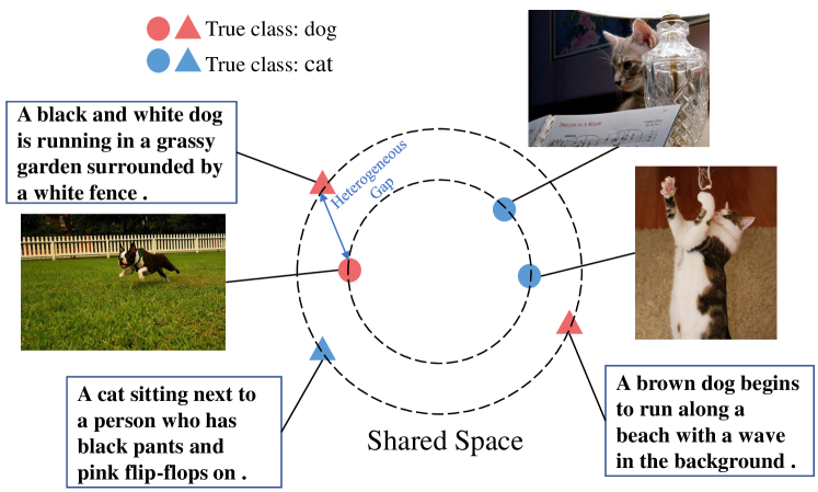
Like many other data-driven tasks, supervised CMR requires massive and high-quality labeled data, which is notoriously labor-intensive. In practice, even for unimodal scenarios, data labeling can suffer from inherent and pervasive label noise, not to mention the extra obstacles from multiple modalities. Taking the image-text pair as an example, while the visual content is intuitive, the semantic label of the textual description is harder to determine due to its subjectivity. Moreover, different modalities lay in separate regions of the shared space and thus exist vast distinctions, which is called heterogeneity gap [10], making learning discriminative representations more difficult. As shown in Fig.1, training with noisy labels would bring two key challenges that enforce the semantically irrelevant data to be similar and widen the heterogeneous gap, which significantly harms the performance of the CMR model. Therefore, endowing supervised CMR methods with robustness against noisy labels is crucial to suit real-world retrieval scenarios.
To mitigate the impact of noisy labels, most of the existing studies attempt to design the robust loss functions [11, 12], reduce the weight of noisy samples [13, 14], select clean samples [15, 16], or generate corrected labels [17, 18]. Despite the success in unimodal scenarios, they cannot directly integrate multiple modalities to cope with the noisy labels in the CMR task. To date, efforts that have been made to achieve robust CMR are still limited. Specifically, MRL [19] combines robust clustering loss and multimodal contrastive loss to combat noisy samples and correlate distinct modalities simultaneously. Inspired by the memorization effect of DNNs [20], ELRCMR [21] introduces an early-learning regularization to further enhance the robustness of clustering and contrasting loss. However, on the one hand, such clustering loss can only down-weight the relative contributions for the incorrect samples, which do not take full advantage of training data. On the other hand, the multimodal contrastive loss only focuses on learning instance-level discriminative representations and neglects the potential semantically relevant data. Thus, the achieved performance by them is argued to be sub-optimal.
To bridge the aforementioned gap, we propose UOT-RCL, a Unified framework based on Optimal Transport for Robust Cross-modal Retrieval. Our UOT-RCL performs both the noisy label problem and multi-modal discrepancy from an OT perspective, leveraging the inherent correlation among multi-modal data to construct effective transport cost. First, to alleviate the influence of noisy labels, we view the label correction procedure as a partial OT problem that progressively transports noisy labeled samples into correct semantics at a minimum cost, where a novel cross-modal consistent cost function is proposed to blend different modalities and provide precise transport cost. To ensure the reliability of the corrected label, we gradually increase the transport mass over the course of training. Second, to narrow the heterogeneous gap of multi-modal data, we model an OT problem to infer the semantic-level matching among distinct modalities, where a relation-based cost function is proposed to preserve the connection of training samples and the selected confident samples. The above two OT-based components can be solved using the efficient Sinkhorn-Knopp algorithm [22] and summarized in one unified framework.
Our main contributions are summarized as follows:
-
•
We propose a novel OT-based framework for supervised CMR with noisy labels, which is a practical but rarely-explored problem in multi-modal learning.
-
•
We present a semantic alignment based on partial OT to progressively correct the noisy labels, where a novel cross-modal consistent cost function is designed to blend different modalities and provide precise transport cost.
-
•
An OT-based relation alignment is proposed to infer the semantic-level cross-modal matching, which is used to narrow the heterogeneous gap among modalities.
-
•
We conduct extensive experiments on three widely used multimodal datasets, which clearly demonstrate the robust performance of our method against noisy labels.
II Related Works
In this section, we briefly review three related topics to our study, including cross-modal retrieval, learning with noisy labels, and optimal transport.
II-A Cross-Modal Retrieval
Cross-modal retrieval aims to retrieve relevant samples from different modalities for a given query. Current dominant methods for CMR is to project distinct modalities into a shared feature space to reduce the heterogeneous gap, wherein the key is to measure the cross-modal similarity. Based on the usage of annotation and retrieval scenes, these methods could be roughly divided into two groups: 1) Unsupervised methods that directly maximize the co-occurred cross-modal agreement between different modalities. One typical research line is global alignment, aiming at learning the correspondence between entire cross-modal data. Existing studies usually adopt a two-stream network to learn comparable global features [23]. Another research line is local alignment which focuses on aligning the local cross-modal regions for more fine-grained CMR. For example, [24, 25] design the cross-attention mechanism to learn alignment between the local regions and words. 2) Supervised methods utilize semantic supervision and aim to constrain the cross-modal instances to be similar for the same category. For example, some methods [26, 27] design the discriminative criteria to maximize the intra-class similarity while minimizing the inter-class similarity. Alternatively, some methods[28, 29] directly utilize a common classifier to enforce multi-modal networks to learn a shared discriminative space. In addition, adversarial learning-based methods [30] typically construct an adversarial process to seek the effective common subspace.
Our proposed approach falls in the category of supervised methods. Despite the success of these prior arts, they heavily rely on well-annotated data and cannot tackle the noise issue. This study aims to find a solution for robust supervised CMR against noisy labels, which is practical but less touched before.
II-B Learning with Noisy Labels
To mitigate the impact of the errors in annotations, numerous approaches have been carried out in past years, which typically consist of sample reweighting, label correction, and noisy sample selection. Sample reweighting methods [31, 13, 14] aim to assign lower weights to potentially noisy labels to reduce their contribution during training. For example, MW-Net [13] learns an explicit loss-weight function in a meta-learning manner. Label correction methods [32, 33] seek to transform noisy labels to correct ones directly, which have shown more favorable results than other methods. DivideMix [34] employs two co-teaching networks to correct targets from the average predictions of different data augmentations. MLC [17] trains a label correction network based on meta-learning to generate corrected labels for training data. Noisy sample selection methods aim to choose and remove noisy labeled data within the training datasets. Existing works are mostly based on the memorization effect of deep networks that samples with higher loss are prone to hold noisy labels and thus exploit the small-loss criterion to divide data. Some recent advances [35, 36] model per-sample loss distribution with mixture probabilistic models to separate noisy samples. Alternatively, some methods [37, 38] resort to neighborhood information in feature space to identify noisy labels. In addition, some state-of-the-art methods combine several techniques to further improve the robustness of models, e.g., ELR [39]. However, most prior arts are designed for the unimodal scenario, and it is difficult or even impossible to apply them to multimodal cases. To combat the noisy labels in CMR, MRL [19] combines two multimodal robust losses to alleviate the influence of noisy samples. ELRCMR [21] introduces a regularization based on early learning to prevent the memorization of noisy labels. Differently, our work tackles this challenge from an optimal transport perspective.
II-C Optimal Transport
Optimal transport is proposed to measure the distance between two probability distributions. One of the factors limiting the widespread application of OT is the high computational cost associated with using linear programming solvers. To improve its availability, entropy-regularized OT [22] is proposed to provide a computationally cheaper solver. Benefiting from this, OT has drawn much attention in various fields of machine learning, which include but are not limited to unsupervised learning [40, 41], semi-supervised learning [42], object detection [43, 44], domain adaptation [45, 46], and long-tailed recognition [47, 48]. Recently, OT-Filter [49] studies the problem of noisy sample selection from the perspective of OT to combat label noise. In contrast, this paper proposes a unified OT-based framework for robust CMR that simultaneously corrects noisy labels and narrows the heterogeneous gap.
III Background
III-A Problem Setup
Without losing generality, we focus on bimodal data, i.e., visual-text pair, to present the noisy label problem in CMR. We assume that there is a collection of visual-text pairs , where is a visual-text pair and is the one-hot semantic label over classes. The goal of supervised CMR is to project the bimodal data into a shared feature space wherein data pairs belonging to the same category have higher feature similarities. Generally, existing methods attempt to learn two modality-specific networks: for visual modality and for text modality, where is the dimension of shared space, and and are the trainable parameters of the two networks. To align cross-modal samples, existing works typically use learnable common prototype corresponding to each class to calculate the probability of -th sample belonging to the -th class:
| (1) |
where is a temperature parameter. Similarly, the probability for text modality is defined in the same manner but uses the text feature . For notation convenience, we denote and as the prediction vectors. Then, the modality-specific networks and can be learned by minimizing the following Cross-Entropy (CE) criterion:
| (2) |
The solution in Eq.(2) brings multimodal points with the same semantic label together. However, since contains noise, minimizing Eq.(2) will wrongly pull close those irrelevant samples and thus impair the cross-modal retrieval performance.
III-B Optimal Transport Theory
Optimal Transport (OT) is to seek an optimal transport plan between two distributions of mass at a minimal cost. Here we briefly introduce the optimal transport theory. More details about OT can be found in [50, 51].
Let be the probability simplex in dimension . Consider two sets of discrete data points and , of which the empirical probability measures are and , where is the Dirac function. Here the weight vector and live in and , respectively. When a meaningful cost function is defined, we can get the cost matrix , where . The discrete optimal transport between probability measures and can be formulated as:
| (3) | ||||
where is the Frobenius dot-product and denotes a -dimensional all-one vector. is the transport polytope that consists of all feasible transport plans. is called the optimal transport plan, of which denotes the amount of transport mass between and in order to obtain the overall minimal cost.
IV Methodology
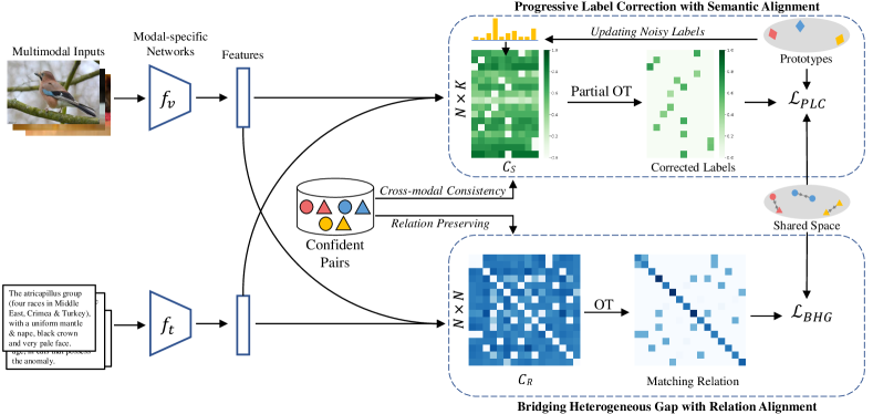
In this section, we present our novel OT-based unified framework for robust cross-modal learning, namely UOT-RCL. As illustrated in Fig.2, UOT-RCL comprises two key components to mitigate the overfitting to noise (Section IV-B) and bridge the multi-modal heterogeneous gap (Section IV-C) respectively, where the two components are based on Optimal Transport and can be summarized in a unified framework.
IV-A Identify Confident Cross-modal Pairs
Our OT-based framework uses the inherent correlation among modalities to facilitate effective transport cost. Given a multi-modal sample, some modalities may provide redundant or even irrelevant information for its semantic class. Thus, we first identify confident samples that have strong cross-modal semantic consistency. Specifically, we measure the discrepancy between the bimodal predicted probabilities by quantifying its Jensen-Shannon divergence (JSD), i.e.,
| (4) |
where is the KL-divergence function. Note that we warm up the training in the first few epochs with to make the networks and prototypes achieve an initial convergence.
After measuring the discrepancy, we identify confident samples with small JSD, i.e., , indicating the bimodal data are very similar. In addition, to avoid the identified samples being concentrated on easy classes, we enforce a class balance prior by selecting samples from each class equally. Due to the presence of label noise, we take an average probability prediction over modalities to approximate the clean class. The confident set belonging to the -th class is defined as:
| (5) |
where is a threshold to ensure class-balanced selecting, which is dynamically defined by the ranked JSD values. Finally, we collect the confident set over all classes as confident cross-modal pairs, i.e., .
IV-B Progressive Label Correction with Semantic Alignment
IV-B1 Cross-modal Consistent Cost Function
To combat label noise, we view the label correction procedure as an OT problem that transports noisy labeled samples to correct semantics at a minimum cost. Denoted the corrected label matrix as , the corresponding cost matrix is desirable to measure the distance between samples and semantic content. can be flexibly defined in different ways; a simple yet effective option is to set , where is a proper prediction matrix, e.g., the model’s predictions [47, 48]. However, estimating reliable predictions is challenging in our scenario. First, the incorrection in the label space imposes formidable obstacles for proper predictions. Second, multiple modalities may contribute differently to the predictions, e.g., the text is usually subjective and contains some redundant description.
To address the above issue, we propose a cross-modal consistent cost function based on the estimation of the contrastive neighbors. Specifically, we first re-estimate the predictive reliability of a candidate sample by contrasting it against its intra-modality nearest neighbors in the feature space. Such contrastive estimation idea is based on the deep clustering [52, 53] that samples with the same semantic content are aggregated in the embedding space. For this goal, given two arbitrary representations and in the shared space, we measure the similarity between them by the cosine distance:
| (6) |
Then, for the cross-modal pair , we contrast each modality with its top- nearest neighbors based on the representation similarity to estimate the clean semantic classes, where the similarity itself is viewed as the clustering weight. To tackle the second challenge, we use the confident pairs to quantify the cross-modal consistency, which is further used to calculate an optimal blending of multi-modal predictions. Taking the visual modality for example, given , we first use as a query to search its intra-modal closet sample from . Since and share the same semantics, the visual consistency can be measured by comparing the closet visual feature distance and the corresponding textual distance:
| (7) |
Similarly, we can calculate its textual consistency by using as a query. Finally, blending the contrastive neighbors estimation with the modal consistency, we define as:
| (8) | ||||
where and denotes the feature-space neighbor set of nearest samples w.r.t. and , respectively.
To enable to be dynamically updated, we propose a softened and moving-average strategy to gradually update the targets:
| (9) |
where is the momentum parameter. The intuition is that the prototype represents the clustering center embedding for the corresponding class and thus can be used to smoothly update the training targets towards accurate ones.
IV-B2 Progressive Label Correction as an OT Problem
As relies on the gradually updated training targets, it cannot completely mitigate the influence of noise, especially in the early stages of training. To this end, we propose to view the label correction procedure as a partial OT problem [42, 54] that seeks only unit mass to be transported between samples and semantic classes, where is progressively increased over the course of training. Such progressive label correction can be formalized as the following objective:
| (10) | ||||
| s.t. | ||||
| (11) | ||||
| (12) | ||||
| (13) |
Here the marginal probability vector represents the expected class distribution, e.g., for a balanced classes. The row constraint Eq.(11) indicates that the training examples are sampled uniformly. The column constraint Eq.(12) enforces the distribution of corrected labels to match the marginal class distribution. The mass constraint Eq.(13) restricted that the corrected labels only assign to -unit most confidently samples based on transport cost. Besides, , , and are the optimizable variables to ensure the objective be feasible. As in Eq.(10) is essentially a joint probability matrix, we re-scaled it to to represent the formal label-space matrix.
Exactly solving Eq.(10) is computationally expensive. Fortunately, it can be transformed into a standard OT problem and be solved by the efficient Sinkhorn-Knopp algorithm[22]. Specifically, we first collect the optimizable variables into and denote the corresponding cost matrix as , i.e.,
where denotes a -dimensional all-zero vector. The row and column marginal projection measures for , i.e., and , is defined as and to satisfy the constraints in Eq.(10), respectively. Based on these, computing the corrected label matrix in partial OT boils down to solving the following standard OT problem:
| (14) | ||||
The optimal transport plan can be solved by the efficient Sinkhorn algorithm that only contains matrix multiplication operations, and our objective = . Then, we can train the modal-specific networks and prototypes robustly with corrected labels:
| (15) |
To increase the strength of corrected samples, we increase the value of as training progresses. While there are several strategies to increase with iteration, we use a linear schedule specified by a start and end value for simplicity.
IV-C Bridging Heterogeneous Gap with Relation Alignment
As mentioned, the core of cross-modal retrieval is to make correlated data from different modalities be similar in the shared space. However, the multi-modal data contains the inherent heterogeneity gap that causes inconsistent representations of various modalities. To learn discriminative representations, recent advances [19, 21] resort to contrastive learning that maximizes the multi-modal mutual information at the instance level. Despite their promise, they view cross-modal data from different instances as irrelevant pairs, which hinders effective supervised CMR, i.e., learning discriminative representations within the semantic classes.
To narrow the heterogeneity gap, we model an OT problem to infer the semantic-level matching among different modalities. In particular, we preserve the relation of each training sample to the set of confident pairs to benefit the transport plan against label noise. For the -th training pair , its visual-modal relation score to the -th confident pair is defined as:
| (16) |
where is a temperature parameter. The textual-modal relation score can be computed analogously. We denote and to represent the relation of and to the confident pairs in visual and textual modalities respectively. Intuitively, if two cross-modal samples share a similar relation to the confident set in the corresponding modality, they can be considered following the same semantic information. Thus, we formalize a relation-based OT problem to seek a proper cross-modal matching , i.e.,
| (17) | ||||
where and are set to that considers the visual and textual samples follow a uniform distribution. We define the relation-based transport cost by based on the Jensen-Shannon divergence.
To learn semantic-level discriminative representations, we use the solved matching relation to align cross-modal samples. Formally, we first define the inter-modal matching probability, i.e., -th textual sample w.r.t. the -th visual query as , where is the temperature parameter. Symmetrically, the matching probability is defined in a similar manner. We denote and as probability vectors. Then, we eliminate the cross-modal discrepancy by maximizing the agreement between different modalities within the same semantics, which can be formulated as the contrastive learning (InfoNCE [55]) loss:
| (18) |
where and be the row-wise and column-wise normalized matching relation for -th sample, respectively.
IV-D The Unified Training Objective
Combined the above analysis, the final loss function can be formulated as:
| (19) |
By minimizing the unified loss function, the modal-specific networks can simultaneously mitigate the impact of noisy-labeled samples and bridge the heterogeneous gap, and thus achieve robust cross-modal retrieval.
V Experiment
In this section, we conduct comprehensive experiments to verify the effectiveness of our proposed method.
V-A Datasets and Evaluation Protocol
V-A1 Datasets.
Without loss of generality, we evaluate our method on three widely-used cross-modal retrieval datasets. The details are introduced as follows:
- •
-
•
NUS-WIDE [58] is a large-scale multi-label dataset containing 269,648 image-text pairs distributed over 81 classes. In the experiments, we employ the same subsets following [19], wherein each pair only belongs to one of ten classes. Specifically, the subsets contain 42,941, 5,000, and 23,661 pairs for training, validation, and testing, respectively.
-
•
XMediaNet [59] is a multimodal dataset consisting of five media types, i.e.image, text, video, audio, and 3D model. Following [19], we select image and text modalities with 200 categories to conduct experiments. Specifically, we randomly divide the dataset into three subsets, i.e.32,000 pairs for training, 4,000 pairs for validation, and 4,000 pairs for testing.
V-A2 Evaluation Protocol.
We evaluate the retrieval performance with the Mean Average Precision (mAP). In a nutshell, mAP measures the accuracy scores of retrieval results, which computes the mean value of Average Precision (AP) for each query, i.e.,
| (20) |
where and denotes true positives and false positives for the -th class, respectively. In our experiments, we take images and texts as queries to retrieve the relevant texts and image samples, respectively. For all methods, we choose the best checkpoint on the validation set and report the corresponding performance on the test set. Following [19], we set the label noise to be symmetric with noise ratios 0.2, 0.4, 0.6, and 0.8 to evaluate the retrieval performance of the methods comprehensively.
V-B Implementation Details
As a general framework, our UOT-RCL can be readily applied to various CMR methods to improve their robustness. For a fair comparison, we employ the same network backbones with MRL [19], i.e. the VGG-19 [60] pre-trained on ImageNet [61] as the backbone for images, the Doc2Vec [62] pre-trained on Wikipedia as the backbone for text, and a three fully-connected layers stacked after the backbones to learn common embeddings among multiple modalities. The dimension of common space is set as 512. For all datasets, the training processes contain 100 epochs, and the warm-up training has 2 epochs. We use Adam as our optimizer, and the learning rate is set to for all experiments. The batch size is set as 100, 500, and 100 for Wikipedia, NUS-WIDE, and XMediaNet, respectively. The temperature parameters , , and are set as 1. The momentum parameter is set as 0.99, and we set the weight factor to 0.4. The number of neighbors is approximately 5‰ of training data, i.e. we set as 10, 200, and 150 for Wikipedia, NUS-WIDE, and XMediaNet, respectively. The number of samples belonging to each class in the confident set is 5 for all experiments. For our progressive label correction process, the mass parameter is linearly increased from 0.2 to 0.8 over the course of training in all experiments.
V-C Comparison with the State-of-the-Art
We compare UOT-RCL with 15 state-of-the-art CMR methods, including four alignment-wise methods (i.e. MCCA [63], PLS [64], DCCA [65], and DCCAE [66]), and ten label-wise methods (i.e. MvDA [67], GSS-SL [68], ACMR [30], deep-SM [69], FGCrossNet [70], SDML [28], DSCMR [29], SMLN [71], MRL [19], and ELRCMR [21]). Note that MRL and ELRCMR are designed to tackle CMR with noisy labels. Table II and Table I present the retrieval mAP scores under a range of noisy label ratios on three datasets, respectively. As shown in these results, we can obtain the following observations:
-
•
Training with noisy labels can remarkably harm the performance of supervised CMR models. As the ratio of label noise increases, the mAP scores of these methods will decrease rapidly.
-
•
Even if the labels are noisy, unsupervised methods are usually inferior to supervised counterparts, which indicates that unsupervised methods are poor at learning semantic-level discriminative representations. However, unsupervised methods work better in the case of extreme noisy labels, i.e., 80% ratio.
-
•
Our method outperforms all existing state-of-the-art methods on all datasets with different noise settings, which shows the superior robustness of UOT-RCL against noisy labels. Moreover, when the noise ratio is high, the improvement of UOT-RCL is more evident, which can be observed in Wikipedia Table II.
-
•
An increased number of classes makes learning with noisy labels more challenging. As shown in Table I, even some robust methods, e.g., MRL, demonstrate a significant performance drop on XMediaNet with high noise. By contrast, our UOT-RCL consistently achieves superior results, e.g., we surpass the best baseline under different noisy settings by 7.4%, 5.7%, 5.9%, and 4.3%, respectively.
| NUS-WIDE | XMediaNet | |||||||||||||||
|---|---|---|---|---|---|---|---|---|---|---|---|---|---|---|---|---|
| Method | Image-to-Text | Text-to-Image | Image-to-Text | Text-to-Image | ||||||||||||
| 0.2 | 0.4 | 0.6 | 0.8 | 0.2 | 0.4 | 0.6 | 0.8 | 0.2 | 0.4 | 0.6 | 0.8 | 0.2 | 0.4 | 0.6 | 0.8 | |
| MCCA | 0.523 | 0.523 | 0.523 | 0.523 | 0.539 | 0.539 | 0.539 | 0.539 | 0.233 | 0.233 | 0.233 | 0.233 | 0.249 | 0.249 | 0.249 | 0.249 |
| PLS | 0.498 | 0.498 | 0.498 | 0.498 | 0.517 | 0.517 | 0.517 | 0.517 | 0.276 | 0.276 | 0.276 | 0.276 | 0.266 | 0.266 | 0.266 | 0.266 |
| DCCA | 0.527 | 0.527 | 0.527 | 0.527 | 0.537 | 0.537 | 0.537 | 0.537 | 0.152 | 0.152 | 0.152 | 0.152 | 0.162 | 0.162 | 0.162 | 0.162 |
| DCCAE | 0.529 | 0.529 | 0.529 | 0.529 | 0.538 | 0.538 | 0.538 | 0.538 | 0.149 | 0.149 | 0.149 | 0.149 | 0.159 | 0.159 | 0.159 | 0.159 |
| GMA | 0.545 | 0.515 | 0.488 | 0.469 | 0.547 | 0.517 | 0.491 | 0.475 | 0.400 | 0.380 | 0.344 | 0.276 | 0.376 | 0.364 | 0.336 | 0.277 |
| MvDA | 0.590 | 0.551 | 0.568 | 0.471 | 0.609 | 0.585 | 0.596 | 0.498 | 0.329 | 0.318 | 0.301 | 0.256 | 0.324 | 0.314 | 0.296 | 0.254 |
| GSS-SL | 0.639 | 0.639 | 0.631 | 0.567 | 0.659 | 0.658 | 0.650 | 0.592 | 0.431 | 0.381 | 0.256 | 0.044 | 0.417 | 0.361 | 0.221 | 0.031 |
| ACMR | 0.530 | 0.433 | 0.318 | 0.269 | 0.547 | 0.476 | 0.304 | 0.241 | 0.181 | 0.069 | 0.018 | 0.010 | 0.191 | 0.043 | 0.012 | 0.009 |
| deep-SM | 0.693 | 0.680 | 0.673 | 0.628 | 0.690 | 0.681 | 0.669 | 0.629 | 0.557 | 0.314 | 0.276 | 0.062 | 0.495 | 0.344 | 0.021 | 0.014 |
| FGCrossNet | 0.661 | 0.641 | 0.638 | 0.594 | 0.669 | 0.669 | 0.636 | 0.596 | 0.372 | 0.280 | 0.147 | 0.053 | 0.375 | 0.281 | 0.160 | 0.052 |
| SDML | 0.694 | 0.677 | 0.633 | 0.389 | 0.693 | 0.681 | 0.644 | 0.416 | 0.534 | 0.420 | 0.216 | 0.009 | 0.563 | 0.445 | 0.237 | 0.011 |
| DSCMR | 0.665 | 0.661 | 0.653 | 0.509 | 0.667 | 0.665 | 0.655 | 0.505 | 0.461 | 0.224 | 0.040 | 0.008 | 0.477 | 0.224 | 0.028 | 0.010 |
| SMLN | 0.676 | 0.651 | 0.646 | 0.525 | 0.685 | 0.650 | 0.639 | 0.520 | 0.520 | 0.445 | 0.070 | 0.070 | 0.514 | 0.300 | 0.303 | 0.226 |
| MRL | 0.696 | 0.690 | 0.686 | 0.669 | 0.697 | 0.695 | 0.688 | 0.673 | 0.523 | 0.506 | 0.393 | 0.311 | 0.530 | 0.520 | 0.415 | 0.325 |
| ELRCMR | 0.694 | 0.692 | 0.684 | 0.671 | 0.694 | 0.693 | 0.689 | 0.673 | 0.525 | 0.523 | 0.502 | 0.455 | 0.535 | 0.532 | 0.516 | 0.482 |
| UOT-RCL | 0.706 | 0.706 | 0.690 | 0.683 | 0.705 | 0.700 | 0.695 | 0.677 | 0.558 | 0.550 | 0.532 | 0.486 | 0.576 | 0.562 | 0.545 | 0.494 |
| Wikipedia | ||||||||
|---|---|---|---|---|---|---|---|---|
| Method | Image-to-Text | Text-to-Image | ||||||
| 0.2 | 0.4 | 0.6 | 0.8 | 0.2 | 0.4 | 0.6 | 0.8 | |
| MCCA | 0.202 | 0.202 | 0.202 | 0.202 | 0.189 | 0.189 | 0.189 | 0.189 |
| PLS | 0.377 | 0.377 | 0.337 | 0.337 | 0.320 | 0.320 | 0.320 | 0.320 |
| DCCA | 0.281 | 0.281 | 0.281 | 0.281 | 0.260 | 0.260 | 0.260 | 0.260 |
| DCCAE | 0.308 | 0.308 | 0.308 | 0.308 | 0.286 | 0.286 | 0.286 | 0.286 |
| GMA | 0.200 | 0.178 | 0.153 | 0.139 | 0.189 | 0.160 | 0.141 | 0.136 |
| MvDA | 0.379 | 0.285 | 0.217 | 0.144 | 0.350 | 0.270 | 0.207 | 0.142 |
| GSS-SL | 0.444 | 0.390 | 0.309 | 0.174 | 0.398 | 0.353 | 0.287 | 0.169 |
| ACMR | 0.276 | 0.231 | 0.198 | 0.135 | 0.285 | 0.194 | 0.183 | 0.138 |
| deep-SM | 0.441 | 0.387 | 0.293 | 0.178 | 0.392 | 0.364 | 0.248 | 0.177 |
| FGCrossNet | 0.403 | 0.322 | 0.233 | 0.156 | 0.358 | 0.284 | 0.205 | 0.147 |
| SDML | 0.464 | 0.406 | 0.299 | 0.170 | 0.448 | 0.398 | 0.311 | 0.184 |
| DSCMR | 0.426 | 0.331 | 0.226 | 0.142 | 0.390 | 0.300 | 0.212 | 0.140 |
| SMLN | 0.449 | 0.365 | 0.275 | 0.251 | 0.403 | 0.319 | 0.246 | 0.237 |
| MRL | 0.514 | 0.491 | 0.464 | 0.435 | 0.461 | 0.453 | 0.421 | 0.400 |
| ELRCMR | 0.515 | 0.503 | 0.496 | 0.447 | 0.460 | 0.456 | 0.447 | 0.416 |
| UOT-RCL | 0.522 | 0.520 | 0.503 | 0.473 | 0.469 | 0.464 | 0.454 | 0.427 |
| Method | XMediaNet | |||||||
|---|---|---|---|---|---|---|---|---|
| Image-to-Text | Text-to-Image | |||||||
| 0.2 | 0.4 | 0.6 | 0.8 | 0.2 | 0.4 | 0.6 | 0.8 | |
| CLIP (RN50) Zero-shot | 0.333 | 0.333 | 0.333 | 0.333 | 0.320 | 0.320 | 0.320 | 0.320 |
| CLIP (ViT-B/16) Zero-shot | 0.358 | 0.358 | 0.358 | 0.358 | 0.370 | 0.370 | 0.370 | 0.370 |
| CLIP (ViT-L/14) Zero-shot | 0.377 | 0.377 | 0.377 | 0.377 | 0.403 | 0.403 | 0.403 | 0.403 |
| CLIP (RN50) Unsupervised fine-tune | 0.655 | 0.655 | 0.655 | 0.655 | 0.660 | 0.660 | 0.660 | 0.660 |
| CLIP (ViT-B/16) Unsupervised fine-tune | 0.738 | 0.738 | 0.738 | 0.738 | 0.738 | 0.738 | 0.738 | 0.738 |
| CLIP (RN50) Supervised fine-tune | 0.674 | 0.599 | 0.481 | 0.250 | 0.681 | 0.614 | 0.520 | 0.293 |
| CLIP (ViT-B/16) Supervised fine-tune | 0.750 | 0.664 | 0.538 | 0.156 | 0.758 | 0.677 | 0.545 | 0.164 |
| CLIP (ResNet50) + UOT-RCL | 0.798 | 0.793 | 0.784 | 0.769 | 0.792 | 0.791 | 0.779 | 0.768 |
| CLIP (ViT-B/16) + UOT-RCL | 0.825 | 0.820 | 0.815 | 0.801 | 0.819 | 0.819 | 0.816 | 0.799 |
V-D Comparison to Large Pre-trained Model
In this section, we perform comparison to the large pre-trained vision-language model, i.e., CLIP [72], which is trained over 400 million image-text pairs and shows powerful performance on transferring downstream tasks. Such a comparison is helpful in understanding how to adapt the large pre-trained model to downstream vision-language retrieval tasks containing noisy supervision. In the experiments, we compare CLIP on the XMediaNet dataset under the following four settings, i.e., zero-shot, unsupervised fine-tune, supervised fine-tune, and combined with our UOT-RCL framework. Specifically, the first setting directly uses trained CLIP models to conduct inference on XMediaNet, the second one uses contrastive learning to align cross-modal representations belonging to the same category from the same pair, the third one uses contrastive learning to align cross-modal representations belonging to the same category, and the last one uses our UOT-RCL framework based on trained CLIP models. All models are trained for 16 epochs with a batch size of 128, and the optimizer settings for fine-tuning follow the CLIP-FT code 111https://github.com/Zasder3/train-CLIP-FT. As shown in Table III, we could observe the following conclusions:
-
•
Although CLIP utilizes massive pairs for pre-training, it focuses on aligning instance-level cross-modal representations and shows noteworthy performance degradation in retrieving category-level cross-modal samples.
-
•
Despite the presence of noisy labels, the supervised fine-tune variants are still superior to unsupervised ones in a low noise ratio, which evidences the importance of supervision in learning semantic category discrimination.
-
•
The capacity of the CLIP models affects the robustness of supervised variants to noisy labels. Larger models are more prone to overfit the noise in a high noise ratio.
-
•
Applying CLIP to our framework can significantly improve its category-level cross-modal retrieval performance, i.e., UOT-RCL improves ViT-B/16 based CLIP by at least 8.1%, 8.1%, 7.7%, and 6.1% in incremental four noisy settings.
V-E Robustness Analysis
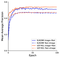
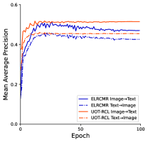
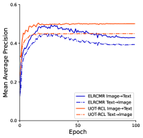
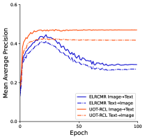
To visually investigate the robustness of the proposed method, we compare the mAP scores of our UOT-RCL and the ELRCMR method on the validation set of Wikipedia under different noise ratios. As shown in Fig.3, one could see that our UOT-RCL surpasses the ELRCMR method in both performance and stability in all noisy settings, which indicates that our method has improved the robustness of the CMR model against noisy labels. Although ELRCMR adopts early learning regularization to prevent memorizing noisy labels, it still tends to overfit with training processes, especially in the high noisy settings, i.e., Fig.3c and Fig.3d. Thanks to our UOT-RCL, which generates corrected labels and narrows the heterogeneous gap, one could greatly improve the robustness of the model to resist extreme noise.
| Method | Image-to-Text | |||
|---|---|---|---|---|
| 0.2 | 0.4 | 0.6 | 0.8 | |
| UOT-RCL | 0.522 | 0.520 | 0.503 | 0.473 |
| UOT-RCL w/o | 0.476 | 0.464 | 0.451 | 0.400 |
| UOT-RCL w/o | 0.504 | 0.499 | 0.474 | 0.399 |
| UOT-RCL w/o confident set | 0.521 | 0.519 | 0.503 | 0.466 |
| Text-to-Image | ||||
| UOT-RCL | 0.469 | 0.464 | 0.454 | 0.427 |
| UOT-RCL w/o | 0.434 | 0.423 | 0.410 | 0.366 |
| UOT-RCL w/o | 0.453 | 0.447 | 0.420 | 0.363 |
| UOT-RCL w/o confident set | 0.465 | 0.461 | 0.450 | 0.425 |
V-F Ablation Study
To study the influence of specific components in our method, we carry out the ablation study on the Wikipedia dataset under different noise ratios. Specifically, we ablate the contributions of three key components in our UOT-RCL, i.e., , , and the confident set. Note that we select random samples into to explore the influence of the confident set. For a fair comparison, all the compared methods are trained with the same settings as our UOT-RCL. As shown in Table IV, one could see that the full UOT-RCL achieves the best performance under different noise ratios, showing that all three components are important to improve the robustness against noisy labels. We could also see that the label correction process, i.e., , has the most important contribution to combat noise. Besides, the contribution of increases with the rise in the noise ratios, which indicates that noisy labels can confuse the discriminative connections among different modalities and widen the heterogeneous gap.
V-G Parameter Analysis
V-G1 Effect of weight factor
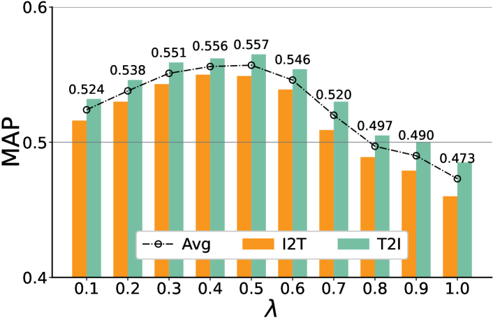
We now investigate the effect of the weight factor by plotting the cross-modal retrieval performance versus on the testing set of XMediaNet in Fig. 6. From the Figure, one could see that both the two components, i.e., semantic alignment () and relation alignment () are important to improve the robustness against noisy labels, which is consisted with the observation in ablation study. In addition, we can also see that UOT-RCL is not sensitive to the selection of . Specifically, our method can obtain decent performance in a relatively larger range of , i.e., 0.1 0.7.
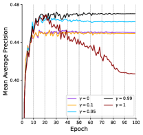
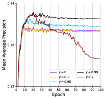
V-G2 Effect of moving-average factor
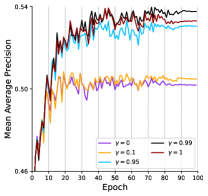
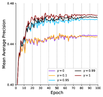
We then explore the effect of training target updating factor on UOT-RCL performance. We set to 0, 0.1, 0.95, 0.99, and 1 to study its influence on retrieval results, where denotes the target is determined entirely by the prototype embeddings, and denotes the target will not be updated and thus the cost matrix is fixed. Fig. 4 shows the learning curves of UOT-RCL on the validation set of Wikipedia. From the figure, we can see that the sensitivity of is different in distinct noisy settings. When the noise ratio is 20%, UOT-RCL can obtain stable performance in different values of , in which a relatively higher (i.e., 0.95, 0.99, and 1) can bring better results. However, when the noise ratio is 80%, can result in overfitting and reduce the model performance. This observation indicates that the cost matrix based only on feature-space neighbors is sub-optimal, and it is effective to make dynamically updated with a moving-average strategy. Furthermore, the over-reliance on prototype embeddings in updating the target can also lead to sub-optimal results (i.e., and ). Overall, setting as 0.99 can achieve superior performance under different noise ratios.
V-H Visualization and Analysis
V-H1 Retrieved Examples
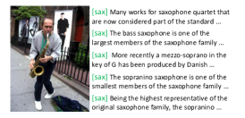
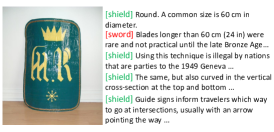
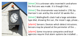
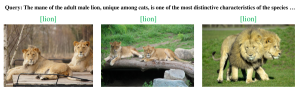
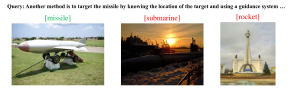
To visually illustrate the retrieval performance of our UOT-RCL, we conduct the case study on the XMediaNet validation set to show some retrieved text and image samples using image queries and text queries, respectively. Specifically, each figure of Figs.5a5c shows a given image query (left) and its top-5 ranked captions (right). Likewise, each figure of Figs.5d5e shows a given caption query (top) and the corresponding top-3 ranked images (bottom). We also highlight the labels of correct retrieval results in green and incorrect ones in red. From these retrieved examples, one could see that our UOT-RCL successfully retrieves most of the relevant items across different modalities. Although some retrieved items do not belong to the same labels as the query data, their semantic content is also correlated with the given queries. For example, the retrieved images in Fig. 5e are all related to weapons, i.e., ”missile”, ”submarine”, and ”rocket”, which are close to the given query. In summary, these retrieval examples show the ability of our method to capture latent semantics for robust CMR.
V-H2 Visualization on the Representations
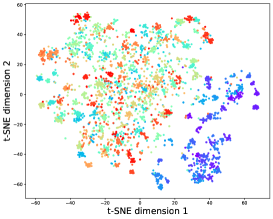
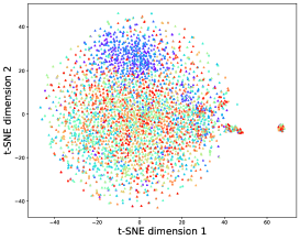
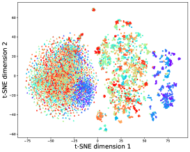
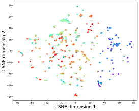
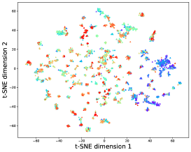
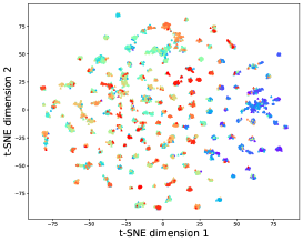
We visualize the visual and textual representation produced by the modal-specific networks using t-SNE in Fig .7. We contrast the t-SNE embeddings of the original features (Figs .7a 7c) and the learned features (Figs .7d 7f). The visualizations of original features show the heterogeneous gap among modalities that the spatial distribution of visual and textual features are significantly different. Besides, we can observe that both the image and text features of UOT-RCL are distributed regularly in semantics and aligned closely across different modalities, which validates the effectiveness of our method in learning semantic-level discriminative representations and bridging the heterogeneous gap. The visualization also shows some learned features with class overlapping due to the presence of noisy labels, which leads to sub-optimal retrieval performance.

V-H3 Visualization on the Corrected Labels
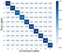
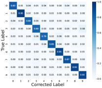
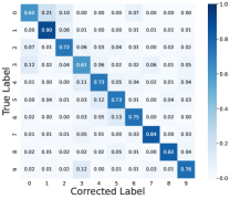
In this section, we carry out experiments on Wikipedia under different noise ratios to visually analyze the accuracy of the corrected labels generated by our UOT-RCL. Fig.8 plots the heatmAP of the probability distribution between the corrected labels and the ground-truth labels on the noisy training set. We can observe that our UOT-RCL successfully generates more reliable corrected labels for all noisy settings. Compared with previous robust methods, i.e., MRL and ELRCMR, trying to down-weight the relative loss for noisy labeled samples, our UOT-RCL goes beyond them by correcting the labels to be reliable, which allows leveraging the training samples more fully.
VI Conclusion
In this paper, we propose to use Optimal Transport to handle the noisy labels and heterogeneous gap in cross-modal retrieval under a unified framework. Our UOT-RCL comprises two key components and uses the inherent correlation among modalities to facilitate effective transport cost. First, to combat noisy labels, we view the label correction procedure as a partial OT problem to progressively correct noisy labels, where a novel cost function is designed to provide a cross-modal consistent cost function. Second, to bridge the heterogeneous gap, we formalize a relation-based OT problem to infer the semantic-level cross-modal matching. Extensive experiments are conducted on several benchmark datasets to verify that our UOT-RCL can endow cross-modal retrieval models with strong robustness against noisy labels.
References
- [1] A. Zheng, M. Hu, B. Jiang, Y. Huang, Y. Yan, and B. Luo, “Adversarial-metric learning for audio-visual cross-modal matching,” IEEE Transactions on Multimedia, vol. 24, pp. 338–351, 2021.
- [2] J. Zhang, Y. Yu, S. Tang, J. Wu, and W. Li, “Variational autoencoder with cca for audio–visual cross-modal retrieval,” ACM Transactions on Multimedia Computing, Communications and Applications, vol. 19, no. 3s, pp. 1–21, 2023.
- [3] S. Zhang, Y. Chen, Y. Sun, F. Wang, H. Shi, and H. Wang, “Lois: Looking out of instance semantics for visual question answering,” IEEE Transactions on Multimedia, 2023.
- [4] S. Sheng, A. Singh, V. Goswami, J. Magana, T. Thrush, W. Galuba, D. Parikh, and D. Kiela, “Human-adversarial visual question answering,” Advances in Neural Information Processing Systems, vol. 34, pp. 20 346–20 359, 2021.
- [5] T. Qian, R. Cui, J. Chen, P. Peng, X. Guo, and Y.-G. Jiang, “Locate before answering: Answer guided question localization for video question answering,” IEEE Transactions on Multimedia, 2023.
- [6] B. Zhu, C.-W. Ngo, and W.-K. Chan, “Learning from web recipe-image pairs for food recognition: Problem, baselines and performance,” IEEE Transactions on Multimedia, vol. 24, pp. 1175–1185, 2021.
- [7] H. Wang, D. Sahoo, C. Liu, K. Shu, P. Achananuparp, E.-p. Lim, and S. C. Hoi, “Cross-modal food retrieval: learning a joint embedding of food images and recipes with semantic consistency and attention mechanism,” IEEE Transactions on Multimedia, vol. 24, pp. 2515–2525, 2021.
- [8] Y. Zhang, W. Ou, Y. Shi, J. Deng, X. You, and A. Wang, “Deep medical cross-modal attention hashing,” World Wide Web, vol. 25, no. 4, pp. 1519–1536, 2022.
- [9] H. Ma, H. Zhao, Z. Lin, A. Kale, Z. Wang, T. Yu, J. Gu, S. Choudhary, and X. Xie, “Ei-clip: Entity-aware interventional contrastive learning for e-commerce cross-modal retrieval,” in Proceedings of the IEEE/CVF Conference on Computer Vision and Pattern Recognition, 2022, pp. 18 051–18 061.
- [10] V. W. Liang, Y. Zhang, Y. Kwon, S. Yeung, and J. Y. Zou, “Mind the gap: Understanding the modality gap in multi-modal contrastive representation learning,” Advances in Neural Information Processing Systems, vol. 35, pp. 17 612–17 625, 2022.
- [11] X. Ma, H. Huang, Y. Wang, S. Romano, S. Erfani, and J. Bailey, “Normalized loss functions for deep learning with noisy labels,” in International conference on machine learning. PMLR, 2020, pp. 6543–6553.
- [12] Z. Sun, F. Shen, D. Huang, Q. Wang, X. Shu, Y. Yao, and J. Tang, “Pnp: Robust learning from noisy labels by probabilistic noise prediction,” in Proceedings of the IEEE/CVF Conference on Computer Vision and Pattern Recognition, 2022, pp. 5311–5320.
- [13] J. Shu, Q. Xie, L. Yi, Q. Zhao, S. Zhou, Z. Xu, and D. Meng, “Meta-weight-net: Learning an explicit mapping for sample weighting,” Advances in neural information processing systems, vol. 32, 2019.
- [14] F. Ma, Y. Wu, X. Yu, and Y. Yang, “Learning with noisy labels via self-reweighting from class centroids,” IEEE Transactions on Neural Networks and Learning Systems, vol. 33, no. 11, pp. 6275–6285, 2021.
- [15] H. Cheng, Z. Zhu, X. Li, Y. Gong, X. Sun, and Y. Liu, “Learning with instance-dependent label noise: A sample sieve approach,” in International Conference on Learning Representations, 2021.
- [16] N. Karim, M. N. Rizve, N. Rahnavard, A. Mian, and M. Shah, “Unicon: Combating label noise through uniform selection and contrastive learning,” in Proceedings of the IEEE/CVF Conference on Computer Vision and Pattern Recognition, 2022, pp. 9676–9686.
- [17] G. Zheng, A. H. Awadallah, and S. Dumais, “Meta label correction for noisy label learning,” in Proceedings of the AAAI Conference on Artificial Intelligence, vol. 35, no. 12, 2021, pp. 11 053–11 061.
- [18] L. Li, L. Chen, Y. Huang, Z. Zhang, S. Zhang, and J. Xiao, “The devil is in the labels: Noisy label correction for robust scene graph generation,” in Proceedings of the IEEE/CVF Conference on Computer Vision and Pattern Recognition, 2022, pp. 18 869–18 878.
- [19] P. Hu, X. Peng, H. Zhu, L. Zhen, and J. Lin, “Learning cross-modal retrieval with noisy labels,” in Proceedings of the IEEE/CVF Conference on Computer Vision and Pattern Recognition, 2021, pp. 5403–5413.
- [20] D. Arpit, S. K. Jastrzebski, N. Ballas, D. Krueger, E. Bengio, M. S. Kanwal, T. Maharaj, A. Fischer, A. C. Courville, Y. Bengio et al., “A closer look at memorization in deep networks,” in ICML, 2017.
- [21] T. Xu, X. Liu, Z. Huang, D. Guo, R. Hong, and M. Wang, “Early-learning regularized contrastive learning for cross-modal retrieval with noisy labels,” in Proceedings of the 30th ACM International Conference on Multimedia, 2022, pp. 629–637.
- [22] M. Cuturi, “Sinkhorn distances: Lightspeed computation of optimal transport,” Advances in neural information processing systems, vol. 26, 2013.
- [23] F. Faghri, D. J. Fleet, J. R. Kiros, and S. Fidler, “Vse++: Improving visual-semantic embeddings with hard negatives,” arXiv preprint arXiv:1707.05612, 2017.
- [24] K.-H. Lee, X. Chen, G. Hua, H. Hu, and X. He, “Stacked cross attention for image-text matching,” in Proceedings of the European conference on computer vision (ECCV), 2018, pp. 201–216.
- [25] K. Li, Y. Zhang, K. Li, Y. Li, and Y. Fu, “Visual semantic reasoning for image-text matching,” in Proceedings of the IEEE/CVF international conference on computer vision, 2019, pp. 4654–4662.
- [26] P. Hu, D. Peng, Y. Sang, and Y. Xiang, “Multi-view linear discriminant analysis network,” IEEE Transactions on Image Processing, vol. 28, no. 11, pp. 5352–5365, 2019.
- [27] P. Hu, D. Peng, X. Wang, and Y. Xiang, “Multimodal adversarial network for cross-modal retrieval,” Knowledge-Based Systems, vol. 180, pp. 38–50, 2019.
- [28] P. Hu, L. Zhen, D. Peng, and P. Liu, “Scalable deep multimodal learning for cross-modal retrieval,” in Proceedings of the 42nd international ACM SIGIR conference on research and development in information retrieval, 2019, pp. 635–644.
- [29] L. Zhen, P. Hu, X. Wang, and D. Peng, “Deep supervised cross-modal retrieval,” in Proceedings of the IEEE/CVF Conference on Computer Vision and Pattern Recognition, 2019, pp. 10 394–10 403.
- [30] B. Wang, Y. Yang, X. Xu, A. Hanjalic, and H. T. Shen, “Adversarial cross-modal retrieval,” in Proceedings of the 25th ACM international conference on Multimedia, 2017, pp. 154–162.
- [31] M. Ren, W. Zeng, B. Yang, and R. Urtasun, “Learning to reweight examples for robust deep learning,” in International conference on machine learning. PMLR, 2018, pp. 4334–4343.
- [32] S. Li, T. Liu, J. Tan, D. Zeng, and S. Ge, “Trustable co-label learning from multiple noisy annotators,” IEEE Transactions on Multimedia, 2021.
- [33] Y. Chen, M. Liu, X. Wang, F. Wang, A.-A. Liu, and Y. Wang, “Refining noisy labels with label reliability perception for person re-identification,” IEEE Transactions on Multimedia, 2023.
- [34] J. Li, R. Socher, and S. C. Hoi, “Dividemix: Learning with noisy labels as semi-supervised learning,” in International Conference on Learning Representations, 2019.
- [35] K. Nishi, Y. Ding, A. Rich, and T. Hollerer, “Augmentation strategies for learning with noisy labels,” in Proceedings of the IEEE/CVF Conference on Computer Vision and Pattern Recognition, 2021, pp. 8022–8031.
- [36] M. Yang, Z. Huang, P. Hu, T. Li, J. Lv, and X. Peng, “Learning with twin noisy labels for visible-infrared person re-identification,” in Proceedings of the IEEE/CVF conference on computer vision and pattern recognition, 2022, pp. 14 308–14 317.
- [37] J. Li, G. Li, F. Liu, and Y. Yu, “Neighborhood collective estimation for noisy label identification and correction,” in Computer Vision–ECCV 2022: 17th European Conference, Tel Aviv, Israel, October 23–27, 2022, Proceedings, Part XXIV. Springer, 2022, pp. 128–145.
- [38] S. Li, X. Xia, S. Ge, and T. Liu, “Selective-supervised contrastive learning with noisy labels,” in Proceedings of the IEEE/CVF Conference on Computer Vision and Pattern Recognition, 2022, pp. 316–325.
- [39] S. Liu, J. Niles-Weed, N. Razavian, and C. Fernandez-Granda, “Early-learning regularization prevents memorization of noisy labels,” Advances in neural information processing systems, vol. 33, pp. 20 331–20 342, 2020.
- [40] M. Caron, I. Misra, J. Mairal, P. Goyal, P. Bojanowski, and A. Joulin, “Unsupervised learning of visual features by contrasting cluster assignments,” Advances in neural information processing systems, vol. 33, pp. 9912–9924, 2020.
- [41] Y. Asano, M. Patrick, C. Rupprecht, and A. Vedaldi, “Labelling unlabelled videos from scratch with multi-modal self-supervision,” Advances in Neural Information Processing Systems, vol. 33, pp. 4660–4671, 2020.
- [42] K. S. Tai, P. D. Bailis, and G. Valiant, “Sinkhorn label allocation: Semi-supervised classification via annealed self-training,” in International Conference on Machine Learning. PMLR, 2021, pp. 10 065–10 075.
- [43] Z. Ge, S. Liu, Z. Li, O. Yoshie, and J. Sun, “Ota: Optimal transport assignment for object detection,” in Proceedings of the IEEE/CVF Conference on Computer Vision and Pattern Recognition, 2021, pp. 303–312.
- [44] T. Afouras, Y. M. Asano, F. Fagan, A. Vedaldi, and F. Metze, “Self-supervised object detection from audio-visual correspondence,” in Proceedings of the IEEE/CVF Conference on Computer Vision and Pattern Recognition, 2022, pp. 10 575–10 586.
- [45] I. Redko, N. Courty, R. Flamary, and D. Tuia, “Optimal transport for multi-source domain adaptation under target shift,” in The 22nd International Conference on Artificial Intelligence and Statistics. PMLR, 2019, pp. 849–858.
- [46] K. Fatras, H. Naganuma, and I. Mitliagkas, “Optimal transport meets noisy label robust loss and mixup regularization for domain adaptation,” in Conference on Lifelong Learning Agents. PMLR, 2022, pp. 966–981.
- [47] H. Peng, M. Sun, and P. Li, “Optimal transport for long-tailed recognition with learnable cost matrix,” in International Conference on Learning Representations, 2022.
- [48] H. Wang, M. Xia, Y. Li, Y. Mao, L. Feng, G. Chen, and J. Zhao, “Solar: Sinkhorn label refinery for imbalanced partial-label learning,” Advances in Neural Information Processing Systems, vol. 35, pp. 8104–8117, 2022.
- [49] C. Feng, Y. Ren, and X. Xie, “Ot-filter: An optimal transport filter for learning with noisy labels,” in Proceedings of the IEEE/CVF Conference on Computer Vision and Pattern Recognition, 2023, pp. 16 164–16 174.
- [50] G. Peyré, M. Cuturi et al., “Computational optimal transport: With applications to data science,” Foundations and Trends® in Machine Learning, vol. 11, no. 5-6, pp. 355–607, 2019.
- [51] C. Villani et al., Optimal transport: old and new. Springer, 2009, vol. 338.
- [52] H. Alwassel, D. Mahajan, B. Korbar, L. Torresani, B. Ghanem, and D. Tran, “Self-supervised learning by cross-modal audio-video clustering,” Advances in Neural Information Processing Systems, vol. 33, pp. 9758–9770, 2020.
- [53] H. Zhang, H. Xu, T.-E. Lin, and R. Lyu, “Discovering new intents with deep aligned clustering,” in Proceedings of the AAAI Conference on Artificial Intelligence, vol. 35, no. 16, 2021, pp. 14 365–14 373.
- [54] L. Chapel, M. Z. Alaya, and G. Gasso, “Partial optimal tranport with applications on positive-unlabeled learning,” Advances in Neural Information Processing Systems, vol. 33, pp. 2903–2913, 2020.
- [55] A. v. d. Oord, Y. Li, and O. Vinyals, “Representation learning with contrastive predictive coding,” arXiv preprint arXiv:1807.03748, 2018.
- [56] N. Rasiwasia, J. Costa Pereira, E. Coviello, G. Doyle, G. R. Lanckriet, R. Levy, and N. Vasconcelos, “A new approach to cross-modal multimedia retrieval,” in Proceedings of the 18th ACM international conference on Multimedia, 2010, pp. 251–260.
- [57] F. Feng, X. Wang, and R. Li, “Cross-modal retrieval with correspondence autoencoder,” in Proceedings of the 22nd ACM international conference on Multimedia, 2014, pp. 7–16.
- [58] T.-S. Chua, J. Tang, R. Hong, H. Li, Z. Luo, and Y. Zheng, “Nus-wide: a real-world web image database from national university of singapore,” in Proceedings of the ACM international conference on image and video retrieval, 2009, pp. 1–9.
- [59] Y. Peng, J. Qi, and Y. Yuan, “Modality-specific cross-modal similarity measurement with recurrent attention network,” IEEE Transactions on Image Processing, vol. 27, no. 11, pp. 5585–5599, 2018.
- [60] K. Simonyan and A. Zisserman, “Very deep convolutional networks for large-scale image recognition,” arXiv preprint arXiv:1409.1556, 2014.
- [61] J. Deng, W. Dong, R. Socher, L.-J. Li, K. Li, and L. Fei-Fei, “Imagenet: A large-scale hierarchical image database,” in 2009 IEEE conference on computer vision and pattern recognition. Ieee, 2009, pp. 248–255.
- [62] J. H. Lau and T. Baldwin, “An empirical evaluation of doc2vec with practical insights into document embedding generation,” in Proceedings of the 1st Workshop on Representation Learning for NLP, 2016, pp. 78–86.
- [63] J. Rupnik and J. Shawe-Taylor, “Multi-view canonical correlation analysis,” in Conference on data mining and data warehouses (SiKDD 2010), 2010, pp. 1–4.
- [64] A. Sharma and D. W. Jacobs, “Bypassing synthesis: Pls for face recognition with pose, low-resolution and sketch,” in CVPR 2011. IEEE, 2011, pp. 593–600.
- [65] G. Andrew, R. Arora, J. Bilmes, and K. Livescu, “Deep canonical correlation analysis,” in International conference on machine learning. PMLR, 2013, pp. 1247–1255.
- [66] W. Wang, R. Arora, K. Livescu, and J. Bilmes, “On deep multi-view representation learning,” in International conference on machine learning. PMLR, 2015, pp. 1083–1092.
- [67] M. Kan, S. Shan, H. Zhang, S. Lao, and X. Chen, “Multi-view discriminant analysis,” IEEE transactions on pattern analysis and machine intelligence, vol. 38, no. 1, pp. 188–194, 2015.
- [68] L. Zhang, B. Ma, G. Li, Q. Huang, and Q. Tian, “Generalized semi-supervised and structured subspace learning for cross-modal retrieval,” IEEE Transactions on Multimedia, vol. 20, no. 1, pp. 128–141, 2017.
- [69] Y. Wei, Y. Zhao, C. Lu, S. Wei, L. Liu, Z. Zhu, and S. Yan, “Cross-modal retrieval with cnn visual features: A new baseline,” IEEE transactions on cybernetics, vol. 47, no. 2, pp. 449–460, 2016.
- [70] X. He, Y. Peng, and L. Xie, “A new benchmark and approach for fine-grained cross-media retrieval,” in Proceedings of the 27th ACM international conference on multimedia, 2019, pp. 1740–1748.
- [71] P. Hu, H. Zhu, X. Peng, and J. Lin, “Semi-supervised multi-modal learning with balanced spectral decomposition,” in Proceedings of the AAAI Conference on Artificial Intelligence, vol. 34, no. 01, 2020, pp. 99–106.
- [72] A. Radford, J. W. Kim, C. Hallacy, A. Ramesh, G. Goh, S. Agarwal, G. Sastry, A. Askell, P. Mishkin, J. Clark et al., “Learning transferable visual models from natural language supervision,” in International conference on machine learning. PMLR, 2021, pp. 8748–8763.
![[Uncaptioned image]](/html/2403.13480/assets/authors/haochen_han.jpg) |
Haochen Han received the B.S. degree from the School of Energy and Power Engineering, Chongqing University, in 2019. Currently, he is a Ph.D. student in the Department of Computer Science and Technology at Xi’an Jiaotong University, supervised by Professor Qinghua Zheng. His research interests include robust multi-modal learning and its applications, such as action recognition and cross-modal retrieval. |
![[Uncaptioned image]](/html/2403.13480/assets/authors/minnan_luo.png) |
Minnan Luo received the Ph. D. degree from the Department of Computer Science and Technology, Tsinghua University, China, in 2014. Currently, she is a Professor in the School of Electronic and Information Engineering at Xi’an Jiaotong University. She was a PostDoctoral Research with the School of Computer Science, Carnegie Mellon University, Pittsburgh, PA, USA. Her research focus in this period was mainly on developing machine learning algorithms and applying them to computer vision and social network analysis. |
![[Uncaptioned image]](/html/2403.13480/assets/authors/huan_liu.jpg) |
Huan Liu received the B.S. and Ph.D. degrees from Xi’an Jiaotong University, Xi’an, China, in 2013 and 2020, respectively. He is currently an Associate Professor with the Department of Computer Science and Technology, Xi’an Jiaotong University. His research interests include affective computing, machine learning, and deep learning. |
![[Uncaptioned image]](/html/2403.13480/assets/x27.png) |
Fang Nan is a Ph.D. student with Faculty of Electronic and Information Engineering, Xi’an Jiaotong University, Xi’an, China. He received the B.E. degree from Xi’an Jiaotong University in 2017. His research interests include computer vision and deep learning. |