Note on Using Singular Value Decomposition to Solve for Single-Phase Flow and Identify Isolated Clusters in Heterogeneous Pore Networks
Abstract
Diluted pore networks or networks that are obtained directly from image analysis are commonly used to evaluate flow through complex porous media. These networks are often subjected to singular points and regions, that is, isolated sub-networks that are not connecting the inlet and outlet. These regions impair the invertibility of the modified Laplacian matrix and affect the accuracy and robustness of pore network models. Searching and eliminating these singularities is commonly done by preconditioning or searching algorithms like breadth-first search or depth-first search. Here, we propose using singular value decomposition (SVD) to simultaneously solve for single-phase flow and locate isolated regions. We demonstrate the performance of the method for networks obtained from images of a partially saturated medium, and for diluted networks close to the percolation threshold.
[inst1]Institute of Environmental Assessment and Water Research (IDAEA), Spanish National Research Council (CSIC), Barcelona, Spain. \affiliation[inst2]Department of Environmental Physics and Irrigation, Institute of Soil, Water and Environmental Sciences, The Volcani Institute, Agricultural Research Organization, Rishon LeZion, Israel
Singular value decomposition (SVD) is an efficient and robust method to solve for single phase flow in heterogeneous networks with isolated clusters
SVD can be used to locate singular points and clusters
Singular value decomposition is robust, and allows for the determination of the percolation threshold in heterogeneous networks.
1 Introduction
Conceptualization of the media as a pore network (rather than a bundle of capillaries) goes back to the work of Fatt [1]. In its simplest form, a porous medium is conceptualized as a lattice of conductors, disregarding the pore shape. More complex (and realistic) pore network models relate the bond geometry to their conductance [2] and map out the pore structure obtained from pore space partitioning [3].
Depending on the flow conditions and complexity of the porous medium, the resulting pore network of the fluid-filled pore space may be characterized by subnetworks or clusters that are hydraulically isolated, that is, clusters that are not connecting the inlet and outlet of the pore network [4]. For example, imbibition or drainage in a porous medium can be modeled as the activation or deactivation of conductors in an equivalent pore network model (PNM) [5]. The probability of a cluster connecting inlet and outlet, can be determined by percolation theory based on the occupation probability () of either lattice bonds or lattice sites and their conductance [6, 7, 5, 8]. Similarly, during dilution of a pore network by randomly eliminating bonds, i.e., assigning zero conductances to them, the resulting network may contain isolated sites. These features cause numerical problems since they lead to singular or ill-conditioned graph Laplacians. This issue is not restricted to diluted regular networks but rather a general issue in any system of linear equations with singular values, such as models derived directly from image analysis of porous and fractured media. In order to address this singularity, different types of iterative search algorithms have been used to find and remove isolated sites and clusters [4, 9].
In this note, we proposed an alternative algorithm based on singular value decomposition (SVD) of the graph Laplacian to identify isolated clusters in the network. SVD decomposes a matrix into the product of a diagonal and two orthonormal matrices [10]. It is used, for example, to determine the pseudoinverse of a singular matrix and calculate low-rank approximations of a matrix. SVD finds broad applications in data-driven science and engineering [11, 12]. The idea here is to use SVD to identify nodes belonging to isolated clusters by solving for single-phase flow in the PNM using the pseudoinverse of the Laplacian matrix. The internal nodes of zero pressure belong to isolated clusters. The proposed method is general and applies to the identification of isolated clusters in networks.
2 Methods
2.1 Graph Laplacian
The graph Laplacian or Kirchoff matrix is a representation of the graph underlying the PNM. The Laplacian here is weighted by the conductances of its bonds of the graph. The conductance or weight matrix contains the conductances between between sites and . If all non-zero conductances are unity, is equal to the adjacency matrix of the graph. The weighted degree matrix is a diagonal matrix that contains the sum of the conductances of the bonds adjacent to a node, that is, , where denotes summation over all sites that are connected to site . With these definitions, the weighted graph Laplacian is given by . The continuity equation for single-phase flow through the PNM can then be written as
| (1) |
where is the vector of pressures at all sites of the network. This can be seen by defining the flow rate between sites and as
| (2) |
which is a statement of momentum conservation. Note that . Continuity, or mass conservation, is expressed by
| (3) |
The latter is equivalent to Eq. (1). The flow rates at sites are defined by
| (4) |
From the mass conservation statement (3), it follows that the graph Laplacian has the eigenvector with the eigenvalue zero, which is the trivial solution of equal pressure at all sites. Thus, the determinant of the graph Laplacian is zero, i.e., is not invertible. The multiplicity of the zero eigenvalue is equal to the number of isolated clusters in the graph, or equivalently, the rank of the graph Laplacian is equal to the number of sites minus the number of connected components[13].
We seek a solution to Eq. (1) for prescribed pressure at the inlet and outlet nodes. To this end, we define the modified graph Laplacian such that for all sites that are in the inlet or outlet boundaries and for all other sites. With this definition, the boundary value problem can be written as
| (5) |
where the vector on the right side of Eq. (5) contains the boundary conditions with for the sites at the inlet boundary and else. For networks that consist of a single connected cluster, the modified Laplacian is an invertible (non-singular) matrix. The trivial zero eigenvalue proper to the graph Laplacian is eliminated by specifying non-trivial boundary conditions. Only in the presence of isolated clusters has the modified graph Laplacian a zero eigenvalue and thus is not invertible. This can be illustrated with the example of a single isolate internal site of the network. In this case, a row in the modified Laplacian is zero and thus, its determinant is zero as well. In order to solve the flow equation (5), and to determine the sites belonging to isolated regions, we use the singular value decomposition.
2.2 Singular Value Decomposition
The singular value decomposition is the decomposition of a diagonal matrix into the product of two orthonormal matrices and and a diagonal matrix with positive real entries as
| (6) |
The entries are called the singular values of . The number of non-zero is defined as the rank of the matrix . The columns of (termed the right singular vectors of ), and the columns of (the left singular vectors), always form an orthogonal set with no assumptions on . If is an invertible matrix, its inverse is given by
| (7) |
If is a singular matrix (i.e., at least one ), its pseudo-inverse is determined as follows [10]. First, the pseudo-inverse of the diagonal matrix is determined by inverting every non-zero element on the diagonal and leaving the zero elements unchanged. In the numerical calculations, elements are inverted if they are larger than a given threshold and set equal to zero if they are smaller. The pseudo-inverse is then given by
| (8) |
Once the pseudo-inverse is obtained, the pressure distribution is determined by a matrix multiplication as
| (9) |
The sites belonging to isolated clusters have zero pressure because they are not connected to inlet and outlet. This approach does not require matrix preconditioning and can be used for singular and invertible matrices. At the same time, it is robust and accurate.
3 Demonstration and Validation
In this section, we demonstrate and validate the proposed SVD approach for two types of media characterized by isolated clusters. First, we consider a pore network obtained by pore space partitioning of an image of the fluid phase of a two-dimensional millifluidic device under partially saturated flow conditions. We use the SVD-based method laid out in Section 2 on the original network to solve the single-phase flow problem (5). The results are compared to the direct inversion of the modified Laplacian in the pore network obtained from pre-conditioned images, in which isolated clusters are removed. The results are compared in terms of relative conductivity, flow rate, and pressure statistics to assess the accuracy of the proposed method. The total flow rate () is defined by the sum of the flow rates at the network’s inlet sites.
| (10) |
We determine the probability density function (PDF) of the flow rate at the sites through areal sampling from the network flow simulations and image pore space partitioning
| (11) |
where [L2] is the area of pore , and is the flow rate at the -th site. The indicator function is one if the flow rate is within the interval and zero otherwise.
The distribution of the pressure at the sites is determined in analogy to the distribution of flow rates
| (12) |
Second, we consider synthetic media obtained by dilution of regular networks. We evaluate the robustness, that is, the ability of the SVD method to solve the flow equation of a media with many singular points and isolated clusters. To this end, we use the SVD method to solve the steady flow equation on two types of diluted networks based on two-dimensional hexagonal and square lattices at different degrees of dilution. We compare the percolation properties determined from the SVD-based flow solution to theoretical values from percolation theory. For this media, it is convenient to evaluate it in terms of relative network conductivity, which is defined in terms of the total flow rate relative to the total flow rate in a corresponding regular network as
| (13) |
where the superscript denotes to the flow rate for the corresponding regular network.
3.1 Pore network from a partially saturated medium
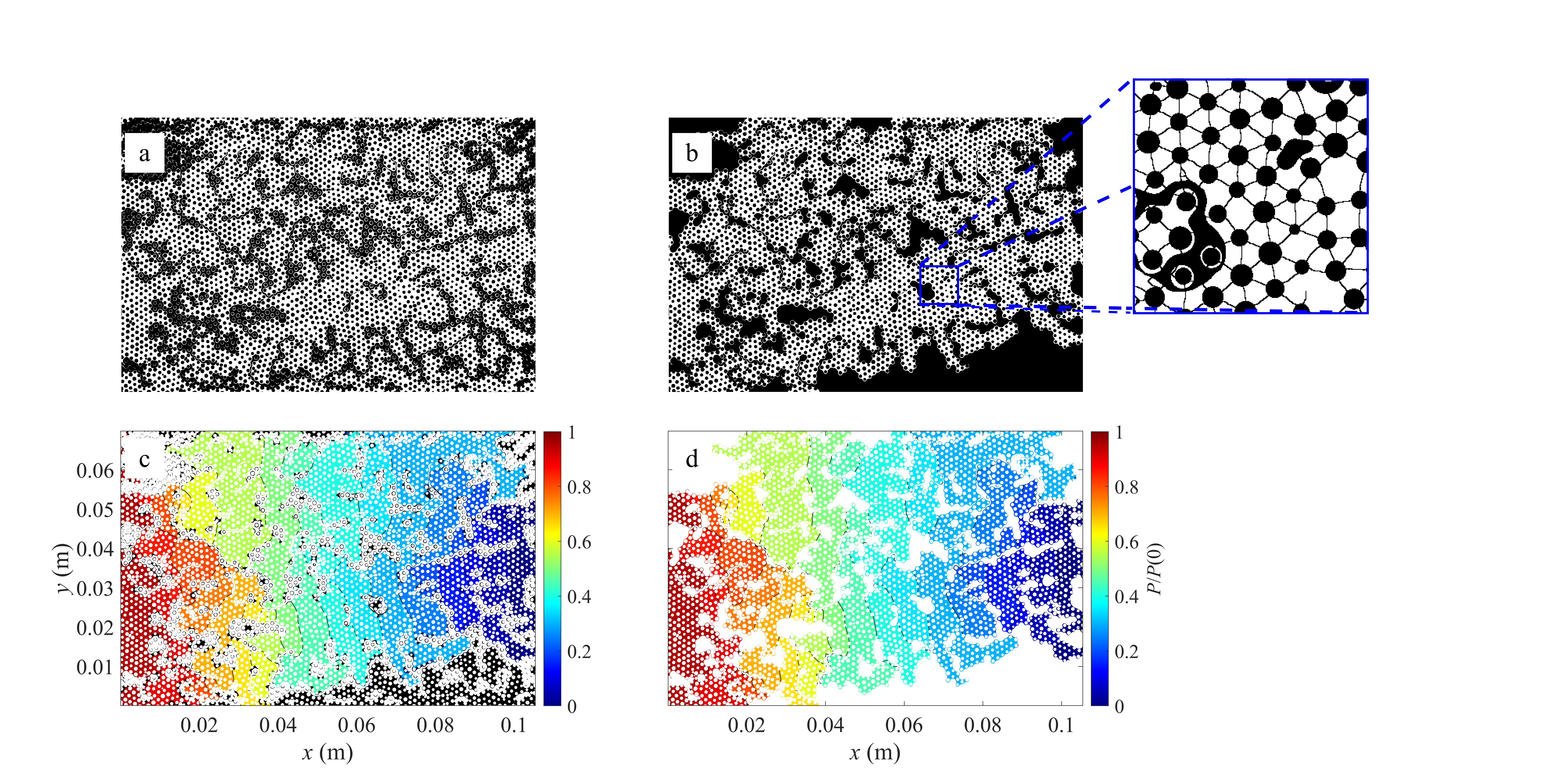
Figure 1 shows the fluid phase (in white) distribution in a milifluidic device before (Fig. 1a) and after (Fig. 1b) processing the image to exclude the non-percolated disconnected fluid clusters. The device is the same used for the experimental work described in [14]. The original image (Fig. 1a) contains many disconnected regions of different sizes. The small regions are formed by wetting liquid phase films surrounding the grains, while the larger clusters are formed by the entrapment of the liquid phase by the non-wetting gas phase. The processed image (Fig. 1b) does not include isolated fluid clusters. The pre-processing of the pixelized image was conducted using the MATLAB image analysis toolbox [15] using the 8-connectivity criterion to identify isolated clusters.
The pore-scale partitioning both in the original and pre-processed images is performed following the methodology presented in [16]. This method uses information about the curvatures of the distance map (obtained from the binary image) to separate distinct pores (small plot in Fig. 1b) and to evaluate the pore body and throat sizes. The construction of the detailed network follows the methodology presented in [17]. A parabolic parameterization of the pore geometry is assumed to evaluate the bond conductivities in the resulting pore network models. For laminar flow, the bond conductance is evaluated by the harmonic sum of the local conductivities along the pore channel with variable width by using Boussinesq [18] equation for rectangular apertures. The pore sizes and conductance distributions and additional information about the milifluidic device and pore partitioning are provided in Figure SF1 in the supplementary material.
As outlined above, for the network constructed from the original image, the flow equation (5) is solved using the pseudoinverse (8) obtained from SVD, which gives the pressures at all sites through Eq.(9). For the network obtained from the pre-processed image, the flow equation is solved by direct inversion of Eq. 5 and by using the pseudoinverse from SVD.
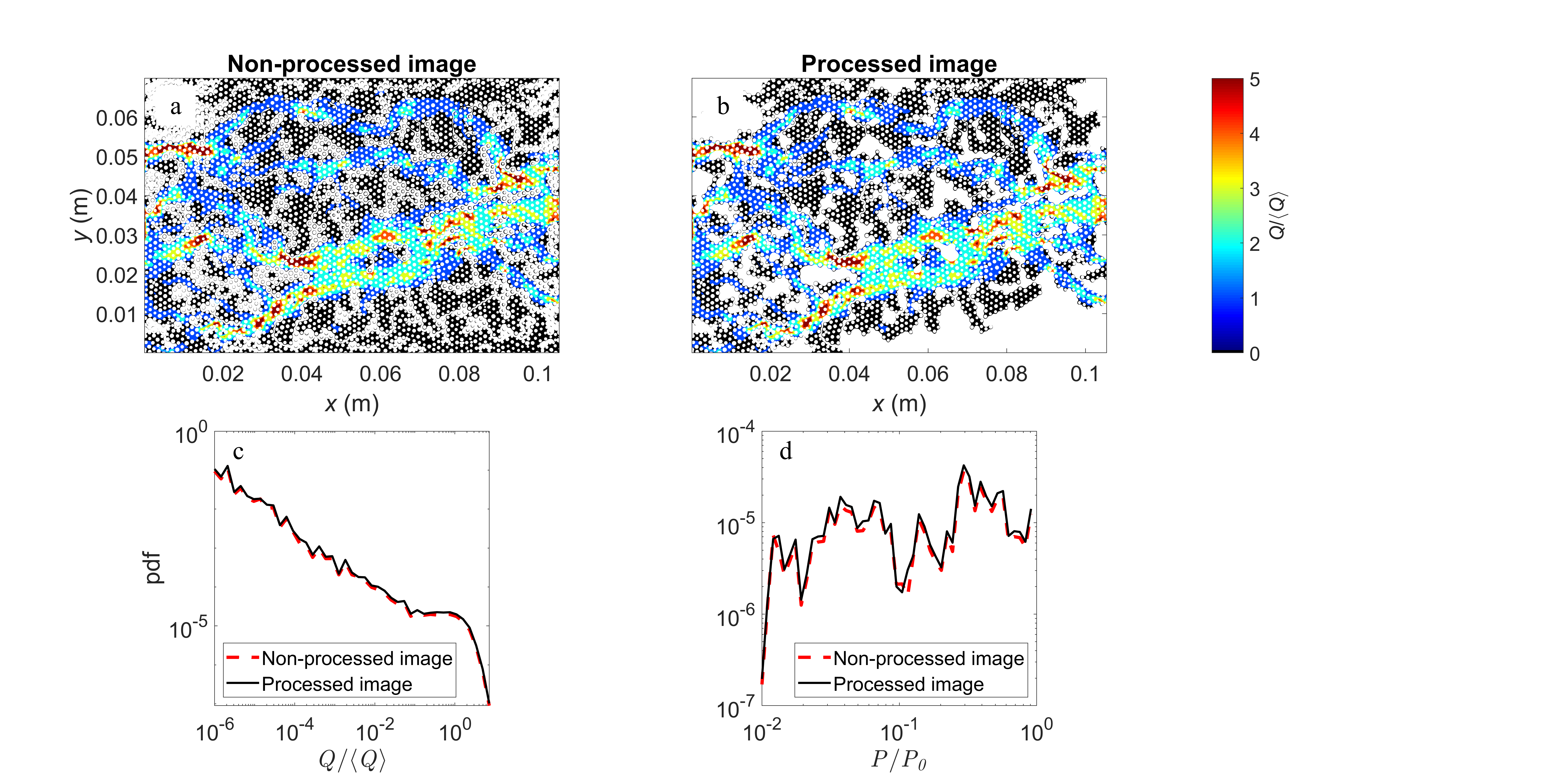
Figure 2a and b show the spatial distribution of flow rates in the pore networks obtained from the original and pre-processed images. The singular disconnected regions attain a zero pressure value. In the network resulting from the original image, the solution using SVD assigns zero pressure to the isolated clusters. The clusters obtained from the SVD analysis on the original image coincide with the clusters identified from the pre-processing step of the binary image. The spatial flow rate distribution in the two networks is essentially identical. This is confirmed by the probability density function of bond flow rates and pressures for both networks, shown in the bottom panel of Figure 2. Moreover, the device flow rate defined in Eq. (10) for the networks from the original and pre-processed images differ by about further confirming the performance and accuracy of the proposed SVD-based method. In order to assess whether this difference is a result of the solution of the flow equation by different methods (SVD versus direct inversion) or due to the pre-processing, we use the SVD method to solve for the flow on the pre-processed image. The difference in the total flow rates obtained by the two methods is smaller than , that is, they are essentially identical. This implies that there is a slight difference in the identification of isolated clusters by the SVD method on the pore network extracted from the direct image and by the connectivity-based method on the pixel image. In other words, the connected percolating clusters in the pore networks extracted from the direct and pre-processed images are not exactly the same. Thus, the SVD-based method provides an accurate method for the identification of isolated clusters and solution of single phase flow in the network obtained from the direct image without the need for pre-processing, which may introduce some inaccuracies.
3.2 Diluted pore networks
Here, we evaluate the ability of the SVD-based method to solve the flow equation and identify isolated clusters at bond occupation probabilities close to the percolation threshold. To this end, we consider two types of diluted lattices based on two-dimensional Hexagonal 2D lattices with coordination number and a two-dimensional square 2D lattice with coordination number . For simplicity, we use a uniform conductance field ( for all ), unit bond length of , sites along each face of the lattices, and a unit pressure gradient . The domain length is for the square lattice, and for the hexagonal lattice, which is oriented with the long diagonal in the main flow direction. The total number of sites in the regular network is denoted by .
Starting from a regular lattice with coordination number , the network is diluted to obtain a target occupation probability
| (14) |
where is the mean coordination number of the diluted network. The dilution method applied here is a simplification of the protocol described in [4]. Each bond is randomly assigned a dilution or elimination number between zero and one. Then, all bonds with an elimination number larger than are assigned zero conductivity. In this way, network realizations are generated for each value. Then, for each realization, the flow equation (5) is solved using the pseudoinverse given by Eq. 8.
We determine for each target value the number of realizations for which a percolating cluster prevails. A percolating cluster exists if the permeability defined by Eq. (13) is larger than 0. The percolation frequency for a given is defined as the ratio of the number of realizations with percolating clusters and the total number of realizations,
| (15) |
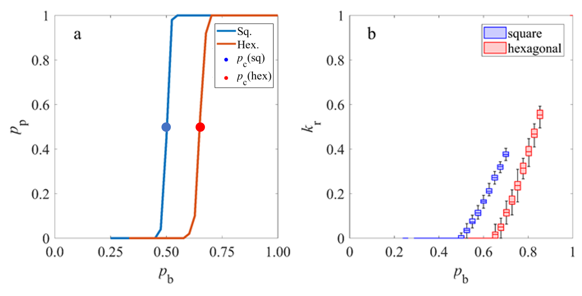
For smaller than a critical value , the bond percolation threshold, there is no percolating cluster, that is, . The theoretical bond percolation threshold for an infinite hexagonal lattice is , and for and infinite square lattice it is [5]. From the SVD-based numerical flow simulations in the diluted networks, the percolation threshold is estimated as the bond occupation probability for which of the lattice realizations percolate [19].
As shown in Figure 3a, the numerical values obtained for are in very good agreement with the theoretical values both for the hexagonal and square lattices. Slight deviation of the numerical from the theoretical values can be attributed to the finite size of the lattices with , and the finite number of realizations with . Figure 3b shows the dependence of permeability on . For , permeability tends to zero, then for it increases monotonically toward , which is the value for the non-diluted lattices. For far from , the evolution is approximately linear. These behaviors are in accordance with the literature [20, 21]. The variability of the values between realizations, illustrated by the width of the error bars, is not linear, with zero variance for and and a large variance for intermediate values. These results demonstrate the robustness of the proposed SVD method.
4 Conclusion
We have shown that SVD is a robust, easy-to-implement, and accurate method to identify sites belonging to isolated clusters in heterogeneous networks. Isolated clusters render the modified graph Laplacian non-invertible. Thus, we use the pseudoinverse determined from SVD to solve for single-phase flow in the heterogeneous networks, which assigns zero pressure to sites belonging to isolated clusters. The SVD method is demonstrated and validated for pore network models of different complexity, which are characterized by singular points and isolated clusters. This shows that SVD provides an alternative to iterative search algorithms for the identification of isolated clusters and a powerful tool to solve for single-phase flow on heterogeneous networks without pre-conditioning.
Acknowledgments
The authors thank Yves Méheust for the image of the milifluidic device. I.B.N, M.D. acknowledge funding from the European Union’s Horizon 2020 research and innovation programme under the Marie Sklodowska-Curie grant agreement No. HORIZON-MSCA-2021-PF-01 (USFT). I.B.N. , J.J.H. and M.D. acknowledge the support of the Spanish Research Agency (10.13039/501100011033), Spanish Ministry of Science, Innovation and Universities through grant HydroPore II PID2022-137652NB-C41. J.J.H. acknowledges the support of the Spanish Research Agency (10.13039/501100011033), the Spanish Ministry of Science and Innovation and the European Social Fund “Investing in your future” through the “Ramón y Cajal” fellowship (RYC-2017-22300).
5 Open Research
No data was used in this research.
References
- Fatt [1956] I. Fatt, The network model of porous media, Transactions of the AIME 207 (1956) 144–177.
- Sahimi [2011] M. Sahimi, Flow and transport in porous media and fractured rock: from classical methods to modern approaches, John Wiley & Sons, 2011.
- Blunt [2017] M. J. Blunt, Multiphase flow in permeable media: A pore-scale perspective, Cambridge university press, 2017.
- Raoof and Hassanizadeh [2010] A. Raoof, S. M. Hassanizadeh, A new method for generating pore-network models of porous media, Transport in porous media 81 (2010) 391–407.
- Hunt and Sahimi [2017] A. G. Hunt, M. Sahimi, Flow, transport, and reaction in porous media: Percolation scaling, critical-path analysis, and effective medium approximation, Reviews of Geophysics 55 (2017) 993–1078.
- Berkowitz and Ewing [1998] B. Berkowitz, R. P. Ewing, Percolation theory and network modeling applications in soil physics, Surveys in Geophysics 19 (1998) 23–72.
- Broadbent and Hammersley [1957] S. R. Broadbent, J. M. Hammersley, Percolation processes: I. crystals and mazes, in: Mathematical proceedings of the Cambridge philosophical society, volume 53, Cambridge University Press, 1957, pp. 629–641.
- Stauffer and Aharony [2018] D. Stauffer, A. Aharony, Introduction to percolation theory, CRC press, 2018.
- Guo et al. [2021] X. Guo, K. Yang, H. Jia, Z. Tao, M. Xu, B. Dong, L. Liu, A new method of central axis extracting for pore network modeling in rock engineering, Geofluids 2021 (2021) 1–20.
- Golub and Van Loan [2013] G. H. Golub, C. F. Van Loan, Matrix computations, JHU press, 2013.
- Brunton and Kutz [2019] S. L. Brunton, J. N. Kutz, Data-Driven Science and Engineering: Machine Learning, Dynamical Systems, and Control, Cambridge University Press, 2019.
- Bisgard [2020] J. Bisgard, Analysis and linear algebra: the singular value decomposition and applications, volume 94, American Mathematical Soc., 2020.
- Bapat [2010] R. B. Bapat, Graphs and matrices, volume 27, Springer, 2010.
- Jiménez-Martínez et al. [2017] J. Jiménez-Martínez, T. Le Borgne, H. Tabuteau, Y. Méheust, Impact of saturation on dispersion and mixing in porous media: Photobleaching pulse injection experiments and shear-enhanced mixing model, Water Resources Research 53 (2017) 1457–1472.
- The MathWorks Inc. [2022] The MathWorks Inc., Matlab version: 9.13.0 (r2022b), 2022. URL: https://www.mathworks.com.
- Ben-Noah et al. [2024a] I. Ben-Noah, J. J. Hidalgo, M. Dentz, Efficient pore space characterization based on the curvature of the distance map, 2024a. arXiv:2403.12591.
- Ben-Noah et al. [2024b] I. Ben-Noah, J. J. Hidalgo, M. Dentz, Evaluation of different network models in variably saturated media, 2024b. arXiv:2403.13519.
- Boussinesq [1868] J. Boussinesq, Mémoire sur l’influence des frottements dans les mouvements réguliers des fluids, Journal de mathématiques pures et appliquées 13 (1868) 377–424.
- Friedman and Seaton [1998] S. Friedman, N. Seaton, Percolation thresholds and conductivities of a uniaxial anisotropic simple-cubic lattice, Transport in porous media 30 (1998) 241–250.
- Kirkpatrick [1973] S. Kirkpatrick, Percolation and conduction, Reviews of modern physics 45 (1973) 574.
- Friedman et al. [1995] S. P. Friedman, L. Zhang, N. A. Seaton, Gas and solute diffusion coefficients in pore networks and its description by a simple capillary model, Transport in porous media 19 (1995) 281–301.