Measurement-only dynamical phase transition of topological and boundary orders
in toric code and gauge-Higgs models
Abstract
We extensively study long-time dynamics and fate of topologically-ordered state in toric code model evolving through a projective measurement-only circuit. The circuit is composed of several measurement operators corresponding to each term of toric code Hamiltonian with magnetic-field perturbations, which is a gauge-fixed version of a (2+1)-dimensional gauge-Higgs model. We employ a cylinder geometry to classify stationary states after long-time measurement dynamics. The appearing stationary states depend on measurement probabilities for each measurement operator. The Higgs, confined and deconfined phases exist in the time evolution by the circuit. We find that both the Higgs and confined phases are clearly separated from the deconfined phase by topological entanglement entropy, whereas the phase boundary between the Higgs and confined phases is obtained by long-range orders on the boundaries supporting the recent observation that the Higgs and confined phases are both one of symmetry-protected-topological states.
I Introduction
Projective measurements performed on quantum circuit generate specific dynamics and produce exotic quantum many-body states. As a recent exciting phenomenon, measurement-induced entanglement phase transition in quantum circuit is attracting attention of broad physicist communities, in which phase transition takes place by the interplay and competition between projective measurements and unitary gates Li2018 ; Skinner2019 ; Li2019 ; Vasseur2019 ; Chan2019 ; Szyniszewski2019 ; Choi2020 ; Bao2020 ; Gullans2020 ; Jian2020 ; Zabalo2020 ; Sang2021 ; Sang2021_v2 ; Nahum2021 ; Sharma2022 ; Fisher2022_rev ; Block2022 ; Liu ; Richter2023 ; Sierant2023 ; Kumer2023 .
Similar measurement-induced phase transitions are also observed in measurement-only circuit (MoC). With suitable choice of measurement operations and their frequencies, MoC generates non-trivial phases of matter; symmetry protected topological (SPT) phases Lavasani2021 ; Klocke2022 ; KI2023 , topological orders Lavasani2021_2 ; Negari2023 , and non-trivial thermal and critical phases Ippoliti2021 ; Sriram2023 ; KOI2023 ; Lavasani2023 ; Zhu2023 . These dynamical phenomena originate from non-commutativity and back action of measurements, and the interplay of them produces intriguing stationary states after ‘time evolution’ through circuit. Furthermore, suitable measurement on initially-prepared states can produce resource states for quantum computation Raussendorf2001 ; Briegel2009 , etc. Example of this ability includes production of long-range entanglement states with intrinsic topological order from simple symmetry-protected-topological (SPT) states Tantivasadakarn2022 .
A recent experiment Google_quantum_AI has realized toric code Kitaev2003 . The robustness of the system to decoherence error, measurements or magnetic perturbation is now open and one of the attracted issues Fan2023 ; Wang2023 .
With the change of geometry of system, how the property of the system changes is an essential issue. For example, in theoretical level, introduction of the cylinder geometry with rough boundary and combination of various types of measurements can exhibit rich physical phenomena to the toric code system Verresen2022 ; Wildeboer2022 ; Negari2023 . Furthermore, there are fascinating findings obtained by interplay between the viewpoint of lattice gauge theory Kogut1979 and the notion of SPT phases Verresen2022 . That is, for the gauge-Higgs model, the boundary state of the cylinder geometry exhibits a kind of long-range order (LRO) with spontaneous symmetry breaking (SSB), and through the SSB pattern, the Higgs and confined phase in the model are to be distinguished, contrary to the common belief that the two phases are adiabatically connected without any transition singularities Fradkin1979 .
The above discussion was obtained by the Hamiltonian formalism. In this paper, we shall study circuit dynamics of toric code system with the cylinder geometry by using measurement-only dynamics. In particular, we investigate how initially-prepared toric code state (topological ordered state) dynamically changes. In this process, the choice of measurement operators and their probability are essential ingredients.
We shall show that rich dynamical behavior and stationary states emerge in the system by varying protocol of the MoC. In particular, we find that Higgs and confined stationary states are separated by a critical line on the boundaries, and then they are explicitly distinguishable in the MoC, in contrast to the well-known conjecture in Fradkin1979 . Furthermore, when we apply strictly competitive measurement protocol for projective measurements, the saturation time gets very long, indicating that competitive dynamics takes place in critical regime among deconfined, Higgs and confined phases. On the other hand, we also observe that topological order (TO) of the initial toric code is sustained by frequent measurement of the toric code stabilizers to eliminate effects of the local projective measurements. This dynamical process can be useful for quantum error correction Botzung .
The rest of this paper is organized as follows. In Sec. II, we explain the setup of MoCs, where two different measurement layers are introduced. Stabilizer generators of the stabilizer formalism, which we employ for the MoC, depend on the cylinder geometry as well as open boundary conditions; upper rough and lower smooth boundaries are used in order to investigate the Higgs and confined phases simultaneously. To clarify the aim of the present study, we also introduce and explain a reference Hamiltonian to the dynamics of this MoC. In the first layer, decoherent single-site (i.e., single-qubit) measurement is performed hindering the TO, whereas the second layer works as recovery of the initial TC state. In Sec. III, We show the practical numerical methods and physical observables to investigate properties of emergent states and their phases. In Sec. IV, we give numerical results of a spin-glass (SG) order of boundary states and its relation to an SPT. Section V displays a numerical study of the bulk TO by employing topological entanglement entropy (TEE). By increasing single-site measurement probability, the initial TC state tends to lose its bulk TO. On the other hand, the boundary SG order emerges. Section VI is devoted to conclusion and discussion.
II Measurement-only circuit and comparable Hamiltonian formalism
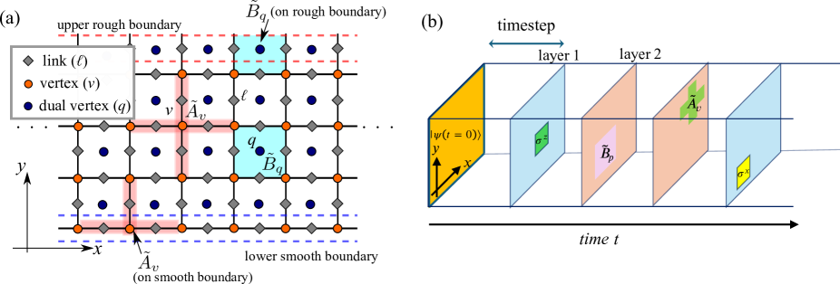
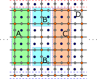
Let us consider a lattice system composed of plaquettes (-lattice) and vortices (-lattice). Physical qubits reside on links of the -lattice. The total qubit number is . We employ cylinder geometry, in which we set the upper rough and lower smooth boundaries in the direction as shown in Fig. 1(a).
We shall investigate ‘time evolution’ of the pure stabilizer state specified by the following set of stabilizer generators Nielsen_Chuang , , where and are the star and plaquette operators of the toric code, defined by and , with standing for links emanating from vertex , and for links composing plaquette . The above stabilizer generators are all linearly independent and specify the stabilizer state , which is nothing but the exact unique gapped ground state of the toric code Hamiltonian without magnetic perturbations on the cylinder geometry degene1 . Throughout this work, we use the same notation for the stabilizer set and the corresponding state interchangeably.
For the stabilizer state of this lattice system, we apply sequential projective measurements as MoC. In the protocol, we introduce two distinct layers: in the first one (called “layer 1”), two projective measurements with observables, and are applied with a uniform probability and , respectively, for each link except the bottom smooth boundary (in the case of ) and each link except the top rough boundary (in the case of ). We choose these measurement points inspired by the Hamiltonian we later commented on Eq. (1).
In the second one (called “layer 2”), two projective measurements with observables, and are applied with the same uniform probabilities for each vertex and plaquette. We consider the following measurement protocol: (I) we choose layer 1 and 2 with probability and , and (II-a) in the case of layer 1, we perform measurement and with probability and , respectively, or (II-b) in the case of layer 2, we perform measurement and with probability . The schematic image of this MoC is shown in Fig. 1 (b). One consecutive application of layers 1 or 2 corresponds to the unit of time.
Dynamics of the MoC and its stationary stabilizer states, if exist, can be inferred from the following Hamiltonian of the toric code model with open boundary conditions and in magnetic fields,
| (1) | |||||
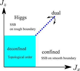
The above model is a gauge-fixing version of a lattice gauge-Higgs model with open boundary conditions employed for investigation on its topological properties KOI2024 . The gauge-Higgs model on infinite system was analyzed in Fradkin and Shenker Fradkin1979 , where the phase diagram with Higgs, confined and deconfined(toric code) regimes was discovered. in Eq. (1) for with general boundary conditions is the fixed point Hamiltonian of the deconfined phase, and its ground states are a gapfull topological state called toric code. The model was recently re-investigated from viewpoint of SPT Verresen2022 , by employing specific boundary conditions. The Higgs and confined phases in (2+1) D can be distinguished with each other by observing the long-range order (LRO) on the boundaries, which is a characteristic signature implying that both the Higgs and confined phases are SPTs being protected by magnetic(electric)-one-form symmetry, respectively. For the Hamiltonian of Eq.(1), we expect a phase diagram such as: Higgs phase for , confined phase for and deconfined(toric code) phase for Trebst2007 ; Vidal2009 ; Tupitsyn2010 ; Dusuel2011 ; Wu2012 . The schematic image of the phase diagram is shown in Fig. 2.
The above phase structure of the Hamiltonian of Eq. (1) gives us insights into the appearance of stationary states in the MoC started with the stabilizer state . In the previous study KI2023 , we investigated relationship between Hamiltonian systems and MoCs. The results obtained there indicate the following relationship between the parameter ratios in the present system, and .
In the recent understanding of the above phase diagram of the gauge-Higgs model, which is an ancestor model of with exactly the same energy eigenstates, higher-form-symmetry plays an important role Gaiotto2015 ; McGreevy2022 . For the case of in in Eq. (1), there emerges magnetic-form-symmetry generated by the operator , where is an arbitrary closed loop on links of the -lattice. Similarly for a string connecting two different links residing on the rough boundary, , is another one-form-symmetry. These one-form-symmetries can be robust for a finite value of as long as the state belongs to the same phase with that of . More precisely, the deconfined(toric code) phase is characterized as an SSB phase of the and symmetries. On the other hand, the Higgs phase is an SPT of the above two symmetries Verresen2022 . For , parallel discussion works for the confined phase as a duality picture and the electric-form-symmetries, and , where links ’s are crossed by and , a close loop and string (connecting two links on the smooth boundary) on the dual lattice, respectively.
III Numerical stabilizer simulation
The projective measurement in the MoC is implemented by the stabilizer formalism Gottesman1997 ; Aaronson2004 . For layer 1; -projective measurement at link removes one of the star operators residing on the boundary vertices of ( and ), and then becomes a stabilizer generator as well as the product of the star operators . That is, the initial stabilizer state tends to lose ’s with the probability , and the number of -stabilizer generator increases instead. Thus, this process leads to decay of the initial TO. Similar process for and with probability .
The projective measurement of layer 2 can be regarded as a recovery process. As explained in Botzung , the projective measurement of () makes () an element of stabilizer generator again by removing local -stabilizer generator if it has been produced by a layer 1 measurement. Thus, we expect that for the case with , the recovery process succeeds in sustaining the TO of the initial state. On the other hand for , stationary states acquire properties of Higgs or confined phase from the viewpoint of the gauge-Higgs model. In particular, in the Hamiltonian picture for Higgs phase (the large- limit), ’s in the bulk get expectation value such as (Higgs condensate), and then the model induces an effective transverse field Ising model Verresen2022 for the degrees of freedom on the upper rough boundary. Thus, it is expected that spontaneous symmetry breaking (SSB) of symmetry takes place on the boundary leading to a magnetic LRO of . A counterpart (dual) picture to the above holds in the confined phase for large because of the electric-magnetic duality, an exact symmetry of the present MoC. A long-range order of emerges on the smooth boundary as a signal of the SPT-confined phase. Beyond the above intuitive pictures, the intermediate regime does not have the magnetic-one-form symmetry nor electric one, and therefore, a sharp SSB of both symmetries might not be observed there. However, detailed Monte Carlo simulations of Gliozzi2006 ; Tupitsyn2010 ; Wu2012 have discovered a very interesting first-order phase transition line in the very vicinity of TO transition, which corresponds to in the present MoC. This point will be discussed after showing numerical calculations of physical quantities.
In the rest of this study, we investigate the above qualitative picture in detail, especially critical regimes separating three phases. The measurement protocol is numerically performed by the efficient numerical simulation by the stabilizer formalism Gottesman1997 ; Aaronson2004 . Throughout this study, we ignore the sign and imaginary factors of stabilizers, which give no effects on observables that we focus on.
This work clarifies the following problems in the MoC; (i) how and when boundary LROs emerge on the upper rough and lower smooth boundaries (ii) how and when the bulk TO disappears. In the numerical study addressing the above problems, we fix and vary up to 26. For the first problem, we calculate the Edward-Anderson SG order parameter Sang2021 defined by
| (2) |
with , where is a stabilizer state and ’s are links on the boundary. As a target observable, we observe the variance of divided by , . This quantity measures sample-to-sample fluctuations and is useful to search a phase transition on the boundary. For the second problem, we calculate topological entanglement entropy (TEE), . In the present study, we employ the partition of the system shown in Fig. 4 Kitaev_Preskill , and for that partition, is defined as
where denote entanglement entropy of the corresponding subsystem, which can be calculated from the number of linearly-independent stabilizers within a target subsystem and the number of qubit of the subsystem Fattal2004 ; Nahum2017 . If the system is an exact topologically-ordered state, we have . The TEE is a useful and standard quantity for investigating bulk TO in the MoC. In particular, even for one of topological degenerate ground states, the TEE works efficiently to observe the TO. In addition, we consider another partition for TEE Levin_Wen , the numerical results of which are given in Appendix B.
IV Dynamics of boundary order parameter
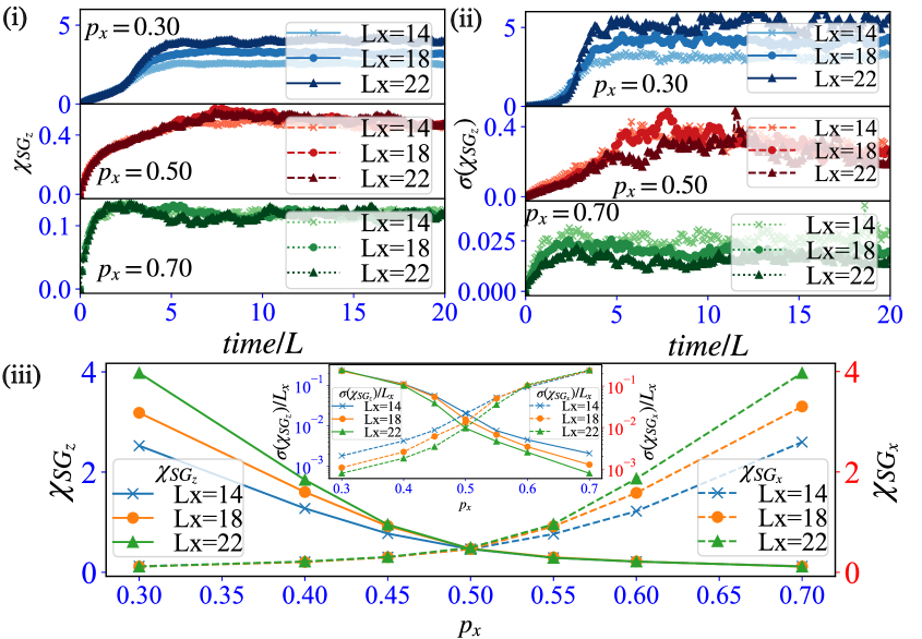
We first observe long-time dynamics of Edward-Anderson SG order for and various values of . For relatively small , the dynamics of is displayed in Fig. 3(i). The value of increases to saturate , signaling a long-range SG order on the upper rough boundary corresponding to the Higgs=SPT phase. There, we also observe large fluctuations as in Fig. 3(ii). From the viewpoint of the Hamiltonian in Eq. (1), the leading term of the present protocol is the -term as , which is nothing but the charged Higgs particle hopping. Then, the coherent Higgs condensation, accompanying Wilson loop condensate, takes place that breaks the TO of the toric code, by the restoration of the magnetic one-form symmetry. The recent studies Verresen2022 showed that this symmetry restoration makes the Higgs phase one of SPTs, which is recognized by observing the degeneracy of the states on the rough boundary, the signal of which has been already verified by numerical methods KOI2024 ; Sukeno2024 . The above finite values of come from the SPT, and then the bulk state is named Higgs=SPT. In passing, as one of the qualitative explanations, another type of symmetry is to be considered KOI2024 , the brief explanation of which is given in Appendix A.
Next for and , in Fig. 3(i) just exhibits a tiny increase and its fluctuations are very small [Fig. 3(ii)]. This result is consistent with the expectation that the Higgs condensate is suppressed for small . Electric-magnetic duality indicates that on the lower smooth boundary exhibits almost the same behavior with on the upper rough boundary for , and we verified this numerically [not shown]. Therefore, condensation of magnetic flux takes place in this parameter region producing the confined phase.
Figure 3(i) shows that the case with and is in between. This regime is simply featureless without any orders. Later study on the TO in the deconfined(toric code) phase will verify this expectation. We also verified that the stable deconfined(toric code) phase emerges for relatively large as a result of the recovery effects.
Finally in Fig. 3(iii), we observe -dependence of the late time value of and for . For small , the late time SG order is enhanced. Close look at behavior of the SG order signifies that a crossover, instead of a phase transition, takes place, i.e., the late time values of smoothly increase with decreasing (increasing) . Further, see the inset of Fig. 3(iii), the variances of and show no significant behavior, mono-increase or decrease. This result is in contrast to the observation for the pure -measurement protocol corresponding to the deconfined(toric code)-Higgs transition studied in the previous paper Ref. KOI2024 . No quantities are indicating a bulk thermodynamic phase transition for the Higgs-confined phase. We expect that this reflects to the behavior of the boundary SG order indicating a novel bulk-boundary correspondence. We explained in the previous study KOI2024 that a finite expectation value of open Wilson loops (EVOWL) generates effective spin couplings on the rough boundary and the SG order emerges as a result. On the deconfined(toric code)-Higgs phase transition, the EVWL (more precisely, Fredenhagen-Marcu string order) exhibits a transition-like behavior similar to the magnetization in the (2+1)D Ising model, whereas in the confined-Higgs crossover regime, both the Wilson and ’t Hooft string symmetries do not emerge as Fradkin-Shenker observation dictates (see also Xu2024 ). Reflecting this smooth change in the bulk properties, the SG order exhibits crossover-like behavior instead of a genuine transition as we observed numerically.
V Dynamics of topological entanglement entropy
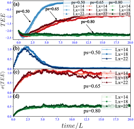
We move on to the dynamics of the TEE. We first study the recovery effect by the measurement of layer 2 for a fixed probability of the measurement of layer 1. The numerical results for various sizes are displayed in Fig. 5 for the most competitive case of layer 1, . For a large recovery case , the TEE starts with and exhibits almost no changes in the long time evolution. The stationary state sustains TO in the bulk staying in the deconfined phase. As shown in Fig. 5 (d), in the whole time evolution, fluctuations are rather small. On the other hand for a relatively weak recovery case with , behavior of the TEE drastically changes from that of large recovery case as seen in Figs. 5 (a) and (b). The late time value of saturates to , indicating that the stationary state loses the initial TO in the bulk. We also find that the fluctuation of the TEE is large in the regime where the TEE changes drastically. This behavior of the TEE in this MoC obviously indicates dynamic phase transition from the deconfnied to Higgs phases. In order to obtain a critical probability, , for the transition, we further observe the late time value of the TEE around and find . The results are displayed in Figs. 5 (a) and (c). There, the saturation value of is fluctuating around and its fluctuation exhibits large values for a long period, exhibiting a small system-size dependence.


Finally, we summarize the saturation vale of as a function of for various system sizes in Fig. 6. We find a clear step-function-like behavior of the TEE and a peak of the fluctuations of the TEE is located at . We expect that in the thermodynamic limit, the saturation value of the TEE becomes a genuine step function of . These results imply that there exists a clear bulk phase transition emerging by varying the recovery probability , at which the bulk topological order vanishes.
We also investigate the behavior of the TEE for a non-contractible partition pattern of the system as in Ref. Levin_Wen , and obtain similar results to the above, which are shown in Appendix B. The initial TC state has for the non-contractible partition, and the state changes its value depending on the probability rates. The critical probability is estimated as for .

VI Conclusion and discussion
The present work clarified the dynamics of MoC, in which we performed competitive measurements on the TC state. There, the measurement operators correspond to the terms in the Hamiltonian of the TC model in magnetic fields. In this MoC, stationary states, which seem to have properties of Higgs, confined and critical phases, emerge by the ‘time evolution’ from the exact stabilizer state of the deconfined (toric code) phase on the cylinder geometry. We identified physical properties of emergent states by numerically observing the boundary long-range magnetic orders and TEE in the bulk. We found that the critical measurement probability ratios corresponds to the ratios of the parameters in the lattice gauge-Higgs model Hamiltonian.
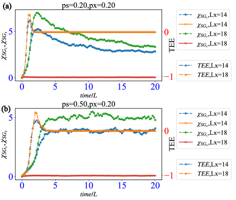
In the present MoC, we observed simultaneously both the SG LRO on the boundary and TEE in the bulk. This gives us an important insight into the relation between the SPT and intrinsic TO in the gauge-Higgs models. As shown in Fig. 7, the ‘time evolution’ of the SG order on the boundaries and TEE in the bulk is observed clearly to find that the bulk topological transition takes place first and the SG transition follows that. This behavior is observed generally. As we explained in the main text, the SG order stems from the bulk one-form-symmetry, in particular, condensation of the Wilson (’t Hooft) string. This condensate induces effective Ising-type long-range couplings between spins on the boundaries producing the SG order. Numerical study in Fig. 7 can be interpreted naturally in such a way that a sufficiently large coupling between boundary spins is necessary for the SG order to emerge. In fact, the recent study on Wilson string condensate for lattice gauge-Higgs model in Ref. Xu2023 shows that the condensate behaves as an order parameter and exhibits Ising spin criticality developing continuously from zero. The difference in the location of the two transitions, which was observed already in our previous work KOI2024 , supports the above observation concerning to the bulk-boundary correspondence.
Acknowledgements
This work is supported by JSPS KAKENHI: JP23KJ0360(T.O.) and JP23K13026(Y.K.).
Appendix A: Non-local gauge invariant operator
To qualitatively understand the boundary LRO in the Higgs phase in the toric code system with the upper rough and lower smooth boundaries on the cylinder geometry, we introduce non-local gauge invariant operator (NLGIO) symmetries for with . Here, we focus on the upper rough boundary and Higgs phase with noticing that parallel argument is possible for the lower smooth boundary and confined phase. Then, the symmetry has two types: (I) with an arbitrary close loop , (II) where and are two arbitrary dangling links on the upper rough boundary and a string in the bulk connecting the and links. Both these operators satisfy for . The second-type NLGIO plays a key role to understand the boundary LRO through the Higgs condensation. That is, the Higgs phase can be regarded as a symmetry-restored state of the second-type NLGIO . In the deep Higgs phase, the local stabilizer generator is proliferated in the bulk, leading to a finite string order, in the system, regarded as the Higgs condensation. As the state of the Higgs phase respects the NLGIO symmetry, then the following relation is satisfied, . That is, the Higgs condensation in the bulk gives the result , the emergence of the LRO on the rough boundary. We expect that the NLGIO symmetries have a similar robustness to the general one-form-symmetry, and the above observation holds for a finite- system as long as it belongs to the Higgs phase. Numerical studies in the present work support this expectation.
We note again that the above discussion of the NLGIO symmetry can be applicable to the emergence of the LRO of on the smooth boundary in the confinement phase by the dual picture.
Appendix B: topological entanglement entropy of another partition
In this Appendix, we show numerical calculations of the TEE employing another type of system partition pattern in Fig. 8. The TEE, , is given by
and for the genuine TC state under this partition and vanishes for a topologically-trivial state. In this pattern of the partition, we are afraid that the TEE exhibits less clear time-evolution behavior than that of in Fig. 5 as the region D is divided into two distinct portions. However, this investigation supports the observation of the TEE obtained for the pattern in Fig. 5, in particular, the location of the phase transition.
References
- (1) Y. Li, X. Chen, and M. P. A. Fisher, Phys. Rev. B 98, 205136 (2018).
- (2) B. Skinner, J. Ruhman, and A. Nahum, Phys. Rev. X 9, 031009 (2019).
- (3) Y. Li, X. Chen, and M. P. A. Fisher, Phys. Rev. B 100, 134306 (2019).
- (4) R. Vasseur, A. C. Potter, Y. -Z. You, and A. W. W. Ludwig, Phys. Rev. B 100, 134203 (2019).
- (5) A. Chan, R. M. Nandkishore, M. Pretko, and G. Smith, Phys. Rev. B 99, 224307 (2019).
- (6) M. Szyniszewski, A. Romito, and H. Schomerus, Phys. Rev. B 100, 064204 (2019).
- (7) S. Choi, Y. Bao, X.-L. Qi, and E. Altman, Phys. Rev. Lett. 125, 030505 (2020).
- (8) Y. Bao, S. Choi, and E. Altman, Phys. Rev. B 101, 104301 (2020).
- (9) C. -M. Jian, Y. -Z. You, R. Vasseur, and A. W. Ludwig, Phys. Rev. B 101, 104302 (2020).
- (10) M. J. Gullans, and D. A. Huse, Phys. Rev. X 10, 041020 (2020).
- (11) A. Zabalo, M. J. Gullans, J. H. Wilson, S. Gopalakrishnan, D. A. Huse, and J. H. Pixley, Phys. Rev. B 101, 060301 (2020).
- (12) S. Sang and T. H. Hsieh, Phys. Rev. Res. 3, 023200 (2021).
- (13) S. Sang, Y. Li, T. Zhou, X. Chen, T. H. Hsieh, and M. P. A. Fisher, PRX Quantum 2, 030313 (2021).
- (14) A. Nahum, S. Roy, B. Skinner, and J. Ruhman, PRX Quantum 2, 010352 (2021).
- (15) S. Sharma, X. Turkeshi, R. Fazio, and M. Dalmonte, SciPost Phys. Core 5, 023 (2022).
- (16) M. P. A. Fisher, V. Khemani, A. Nahum, and S. Vijay, Annu. Rev. Condens. Matter Phys. 14:1, 335-379 (2023).
- (17) M. Block, Y. Bao, S. Choi, E. Altman, and N. Y. Yao, Phys. Rev. Lett. 128, 010604 (2022).
- (18) H. Liu, T. Zhou, and X. Chen, Phys. Rev. B 106, 144311 (2022).
- (19) J. Richter, O. Lunt, and A. Pal, Phys. Rev. Res. 5, L012031 (2023).
- (20) P. Sierant, M. Schirò, M. Lewenstein, and X. Turkeshi, arXiv:2306.04764 (2023).
- (21) A. Kumar, K. Aziz, A. Chakraborty, A. W. W. Ludwig, S. Gopalakrishnan, J. H. Pixley, and R. Vasseur, arXiv:2310.03078 (2023).
- (22) A. Lavasani, Y. Alavirad, and M. Barkeshli, Nat. Phys. 17, 342 (2021).
- (23) K. Klocke and M. Buchhold, Phys. Rev. B 106, 104307 (2022).
- (24) Y. Kuno and I. Ichinose, Phys. Rev. B 107, 224305 (2023).
- (25) A. Lavasani, Y. Alavirad, and M. Barkeshli, Phys. Rev. Lett. 127, 235701 (2021).
- (26) A. -R. Negari, S. Sahu, and T. H. Hsieh, arXiv:2307.02292.
- (27) Y. Kuno, T. Orito, and I. Ichinose, Phys. Rev. B 108, 094104 (2023).
- (28) M. Ippoliti, M. J. Gullans, S. Gopalakrishnan, D. A. Huse, and V. Khemani, Phys. Rev. X 11, 011030 (2021).
- (29) A. Sriram, T. Rakovszky, V. Khemani, and M. Ippoliti, Phys. Rev. B 108, 094304 (2023).
- (30) A. Lavasani, Z. X. Luo, S Vijay, Phys. Rev. B 108, 115135 (2023).
- (31) G. -Y. Zhu, N. Tantivasadakarn, S. Trebst, arXiv:2303.17627 (2023).
- (32) R. Raussendorf and H. J. Briegel, Phys. Rev. Lett. 86 5188 (2001).
- (33) H. J. Briegel, D. E. Browne, W. Dür, R. Raussendorf and M. Van den Nest, Nat. Phys. 5 19 (2009).
- (34) N. Tantivasadakarn, R. Thorngren, A. Vishwanath, and R. Verresen, arXiv:2112.01519 (2022).
- (35) Google quantum AI, Nature 614, 676 (2023).
- (36) A. Y. Kitaev, Ann. Phys. (NY) 303, 2 (2003).
-
(37)
R. Fan, Y. Bao, E. Altman, and A. Vishwanath,
arXiv:2301.05689 (2023). - (38) Z. Wang, Z. Wu, and Z. Wang, arXiv:2307.13758 (2023).
- (39) R. Verresen, U. Borla, A. Vishwanath, S. Moroz, and R. Thorngren, arxiv:2211.01376 (2022).
- (40) J. Wildeboer, T. Iadecola, and D. J. Williamson, PRX Quantum 3, 020330 (2022).
- (41) J. B. Kogut, Rev. Mod. Phys. 51, 659 (1979).
- (42) E. Fradkin and S. H. Shenker, Phys. Rev. D 19, 3682 (1979).
- (43) T. Botzung, M. Buchhold, S. Diehl, and M. Müller, arXiv:2311.14338 (2023).
- (44) M. A. Nielsen and I. L. Chuang, Quantum Computation and Quantum Information, Cambridge, UK: Cambridge University Press, 2010 (2010).
- (45) The degeneracy of exact ground states of the toric code depends on the system geometry. For cylinder with both upper and lower same rough or smooth boundaries, two fold degeneracy appears. Also if we consider square geometry with left and right smooth boundaries and upper and lower rough boundaries, the two-fold degeneracy appears known as a subsystem code Poulin2005 ; Wildeboer2022 ; KI2023 .
- (46) Y. Kuno, T. Orito, and I. Ichinose, Phys. Rev. B 109, 054432 (2024).
- (47) S. Trebst, P. Werner, M. Troyer, K. Shtengel, and C. Nayak, Phys. Rev. Lett. 98, 070602 (2007).
- (48) J. Vidal, S. Dusuel, and K. P. Schmidt, Phys. Rev. B 79, 033109 (2009).
- (49) I. S. Tupitsyn, A. Kitaev, N. V. Prokof’ev and P. C. E. Stamp, Phys. Rev. B 82, 085114 (2010).
- (50) S. Dusuel, M. Kamfor, R. Orús, K. P. Schmidt, and J. Vidal, Phys. Rev. Lett. 106, 107203 (2011).
- (51) F. Wu, Y. Deng, and N. Prokof’ev, Phys. Rev. B 85, 195104 (2012).
- (52) D. Gaiotto, A. Kapustin, N. Seiberg, and B. Willet, JHEP 02 172, 1412.5148 (2015).
- (53) J. McGreevy, Annu. Rev. Condens. Matter Phys. 14, 57 (2023).
- (54) D. Gottesman, arXiv:9807006 (1997).
- (55) S. Aaronson and D. Gottesman, Phys. Rev. A 70, 052328 (2004).
- (56) F. Gliozzi, Nucl. Phys. B Proc. Suppl. 153, 120 (2006).
- (57) A. Kitaev and J. Preskill, Phys. Rev. Lett. 96, 110404 (2006).
- (58) D. Fattal, T. S. Cubitt, Y. Yamamoto, S. Bravyi, and I. L. Chuang, arXiv:0406168 (2004).
- (59) A. Nahum, J. Ruhman, S. Vijay, and J. Haah, Phys. Rev X 7, 031016 (2017).
- (60) M. Levin and X. -G. Wen, Phys. Rev. Lett. 96, 110405 (2006).
- (61) H. Sukeno, K. Ikeda, and T. C. Wei, arXiv:2402.11738.
- (62) W.-T. Xu, F. Pollmann, and M. Knap, arXiv:2402.00127 (2024).
- (63) W. -T. Xu, M. Knap, and F. Pollmann, arXiv:2311.16235 (2023).
- (64) D. Poulin, Phys. Rev. Lett. 95, 230504 (2005).