Bound-Preserving Framework for Central-Upwind Schemes for General Hyperbolic Conservation Laws

Abstract.

Central-upwind (CU) schemes are Riemann-problem-solver-free finite-volume methods widely applied to a variety of hyperbolic systems of PDEs. Exact solutions of these systems typically satisfy certain bounds, and it is highly desirable or even crucial for the numerical schemes to preserve these bounds. In this paper, we develop and analyze bound-preserving (BP) CU schemes for general hyperbolic systems of conservation laws. Unlike many other Godunov-type methods, CU schemes cannot, in general, be recast as convex combinations of first-order BP schemes. Consequently, standard BP analysis techniques are invalidated. We address these challenges by establishing a novel framework for analyzing the BP property of CU schemes. To this end, we discover that the CU schemes can be decomposed as a convex combination of several intermediate solution states. Thanks to this key finding, the goal of designing BPCU schemes is simplified to the enforcement of four more accessible BP conditions, each of which can be achieved with the help of a minor modification of the CU schemes. We employ the proposed approach to construct provably BPCU schemes for the Euler equations of gas dynamics. The robustness and effectiveness of the BPCU schemes are validated by several demanding numerical examples, including high-speed jet problems, flow past a forward-facing step, and a shock diffraction problem.

1. Introduction

This paper focuses on the development of high-order robust numerical schemes for hyperbolic systems of conservation laws

(1.1) $${\bm{u}}_{t}+\nabla_{\bm{x}}\cdot{\bm{f}}({\bm{u}})=\bm{0},$$

where ${\bm{x}}\in\mathbb{R}^{d}$ are the spatial variables, $t\in\mathbb{R}^{+}$ denotes time, ${\bm{u}}\in\mathbb{R}^{m}({\bm{x}},t)$ is an unknown vector-function, and ${\bm{f}}=(f_{1},\dots,f_{d})^{\top}\in(\mathbb{R}^{m})^{d}$ are the fluxes.

Exact solutions of (1.1) often satisfy certain bounds that define a convex invariant region ${\mathcal{G}}\in\mathbb{R}^{m}$. For instance, the entropy solution of scalar conservation laws satisfies the maximum principle, which means that it always stays within the invariant region ${\mathcal{G}}=[\min_{{\bm{x}}}{\bm{u}}({\bm{x}},0),\max_{{\bm{x}}}{\bm{u}}({\bm{x}},0)]$. For the Euler equations of gas dynamics, the corresponding invariant region ${\mathcal{G}}$ includes all admissible states with positive density and pressure. For notational convenience, we assume that the convex invariant region ${\mathcal{G}}$ of equation (1.1) can be expressed as

$${\mathcal{G}}:=\big{\{}\,{\bm{u}}\in\mathbb{R}^{m}:\varphi_{i}({\bm{u}})>0,i\in\mathbb{I}~{}~{}\mbox{and}~{}~{}\varphi_{i}({\bm{u}})\geq 0,i\in\hat{\mathbb{I}}\,\big{\}}$$

with continuous functions $\{\varphi_{i}({\bm{u}})\}$. It is highly desirable or even crucial to ensure that the numerical solutions of (1.1) also stay within the invariant region ${\mathcal{G}}$.

It is well-known that for scalar conservation laws, first-order monotone schemes are bound-preserving (BP) under a suitable CFL condition. Some of these first-order schemes have also been shown to be BP for many hyperbolic systems. However, constructing high-order accurate BP schemes is a considerably more challenging task. A general framework for constructing high-order BP discontinuous Galerkin and finite-volume schemes was proposed in [50, 49] for rectangular meshes, and later extended to triangular meshes in [47]. In this framework, high-order schemes were reformulated as convex combinations of first-order BP schemes, resulting in the BP property of high-order schemes through the convexity of the invariant region. This framework has been extensively applied to various hyperbolic systems; see, e.g., [41, 29, 51, 25, 48, 31, 15, 6, 7]. Another approach for constructing high-order BP schemes is the BP flux limiting approach [44, 13], which aims to design a suitable convex combination of a first-order BP flux and a high-order flux to achieve both the BP property and a high order of accuracy simultaneously. This approach has been successfully applied to various conservation laws, including scalar conservation laws [44], compressible Euler equations [13, 42], and special relativistic hydrodynamics [39]. For more developments on high-order BP schemes, we refer the reader to [46, 43, 11, 45].

Another challenge in analyzing and constructing BP schemes lies in the complexity of invariant region ${\mathcal{G}}$, which may exhibit very complicated explicit formula involving high nonlinearity, not to mention the cases where it can only be defined implicitly [34]. Recently, motivated by a series of BP efforts [40, 32, 33, 37, 38] for magnetohydrodynamic (MHD) equations, the geometric quasilinearization (GQL) framework was proposed in [34] to address BP problems involving highly nonlinear or even implicit constraints. The GQL approach was also applied in [35] to design BP schemes that preserve the invariant region for relativistic hydrodynamics. In addition, the GQL framework was utilized in [36] to explore BP central discontinuous Galerkin schemes for the ideal MHD equations.

Central-upwind (CU) schemes belong to the class of Riemann-problem-solver-free Godunov-type schemes. Compared with the staggered central schemes [1, 14, 21, 23, 24], CU schemes incorporate an upwinding information on local speeds of propagation to reduce the amount of numerical dissipation present in staggered central schemes and to admit a particularly simple semi-discrete form. CU schemes were introduced in [16, 17, 18] and then, in [20], where a more accurate projection step was proposed, leading to a “built-in” anti-diffusion term. The numerical dissipation present in CU schemes was further reduced by modifying the CU numerical fluxes using the local characteristic decomposition [3] and by implementing a subcell approach in the projection step, which leads to a modified, more sharper “built-in” anti-diffusion term [19]. The latter two CU schemes, however, cannot be viewed as “black-box” solvers for general hyperbolic systems of conservation laws as they are constructed for each particular system. Therefore, in this paper, we focus on the CU schemes from [20] and their two-dimensional (2-D) modification from [4].

CU schemes have been applied to various hyperbolic conservation laws or balance laws and it was shown that they satisfy some of the BP properties such as positivity preserving of the density for the Euler equations of gas dynamics and water depth for a variety of shallow water and related models. This paper presents a novel generic framework for analyzing and constructing BPCU schemes for general hyperbolic systems of conservation laws. The main challenges in achieving this goal arise from the presence of the “built-in” anti-diffusion terms, which makes it impossible to recast the CU schemes as convex combinations of first-order BP schemes, thereby invalidating some standard BP analysis techniques. In order to overcome these challenges, we introduce a novel convex decomposition of the CU schemes and find a sufficient condition of the desired BP property. Thanks to this key discovery, the goal of constructing BPCU schemes is simplified into four more accessible tasks, each of which can be accomplished by suitable adjustments to the original CU schemes. Our findings in this paper include the following:

• We propose a novel convex decomposition of the CU schemes, which rewrites them as a convex combination of several intermediate solution states. This formulation overcomes the challenge posed by the complex formula of the CU numerical fluxes and facilitates the BP property analysis;

• We establish a sufficient condition for the BP property of the CU schemes, which only requires the BP property of the intermediate solution states. This finding decomposes the goal of constructing BPCU schemes into four more accessible tasks;

• We develop a BP framework for CU schemes that summarizes our findings. This framework includes a step-by-step procedure for modifying the original CU schemes into BPCU schemes, as well as a set of theoretical results that can be used to prove rigorously the BP property of the BPCU schemes. This BP framework is applicable to general hyperbolic systems of conservation laws;

• We apply the proposed BP framework to construct provably BPCU schemes for the Euler equations of gas dynamics. The analysis of these BPCU schemes is novel and nontrivial, involving both technical estimates and the GQL approach;

• We implement our BPCU schemes and demonstrate their robustness and effectiveness on several demanding numerical examples including high-speed jet problems, flow past a forward-facing step, and a shock diffraction problem.

This paper is organized as follows. In §2, we discuss the one-dimensional (1-D) BPCU schemes. Specifically, we provide a review of the 1-D CU schemes in §2.1; propose the BP framework for the 1-D CU schemes in §2.2; and utilize the BP framework to construct the BPCU scheme for 1-D Euler equations of gas dynamics in §2.3. In §3, we extend the BP framework to the 2-D case. Several numerical tests are presented in §4 to demonstrate the effectiveness and robustness of the proposed BPCU schemes. Finally, we conclude the paper in §5 by summarizing our contributions.

2. One-Dimensional BPCU Schemes

2.1. CU Schemes: a Brief Overview

In this section, we provide a brief overview of the 1-D CU scheme from [20] for

(2.1) $${\bm{u}}_{t}+{\bm{f}}({\bm{u}})_{x}=\bm{0}.$$

Let $\big{\{}\Omega_{j}:=[x_{j-\frac{1}{2}},x_{j+\frac{1}{2}}]\big{\}}$ be a uniform partition of the 1-D spatial domain with the spatial step-size $\Delta x=x_{j+\frac{1}{2}}-x_{j-\frac{1}{2}}$. We denote by $\,\hbox{\vbox{\hrule height=0.5pt\kern 1.29167pt\hbox{\kern-0.50003pt${\bm{u}}$\kern-0.50003pt}}}^{\,n}_{j}$ the approximation of the cell average of ${\bm{u}}(x,t)$ in the cell $\Omega_{j}$ at the time level $t=t^{n}$. With the discussion on high-order temporal discretizations deferred to 2.11, we first consider the semi-discrete CU scheme coupled with forward Euler temporal discretization, namely,

(2.2) $$\hbox{\vbox{\hrule height=0.5pt\kern 1.29167pt\hbox{\kern-0.50003pt${\bm{u}}$\kern-0.50003pt}}}^{\,n+1}_{j}=\,\hbox{\vbox{\hrule height=0.5pt\kern 1.29167pt\hbox{\kern-0.50003pt${\bm{u}}$\kern-0.50003pt}}}^{\,n}_{j}-\lambda^{n}\big{(}\hat{\bm{f}}_{j+\frac{1}{2}}-\hat{\bm{f}}_{j-\frac{1}{2}}\big{)},\quad\lambda^{n}:=\frac{\Delta t^{n}}{\Delta x},~{}~{}\Delta t^{n}:=t^{n+1}-t^{n}$$

with the CU numerical fluxes

(2.3) $$\hat{\bm{f}}_{j+\frac{1}{2}}=\frac{\sigma^{+}_{j+\frac{1}{2}}{\bm{f}}\big{(}{\bm{u}}^{-}_{j+\frac{1}{2}}\big{)}-\sigma^{-}_{j+\frac{1}{2}}{\bm{f}}\big{(}{\bm{u}}^{+}_{j+\frac{1}{2}}\big{)}}{\sigma^{+}_{j+\frac{1}{2}}-\sigma^{-}_{j+\frac{1}{2}}}+\frac{\sigma^{+}_{j+\frac{1}{2}}\sigma^{-}_{j+\frac{1}{2}}}{\sigma^{+}_{j+\frac{1}{2}}-\sigma^{-}_{j+\frac{1}{2}}}\big{(}{\bm{u}}^{+}_{j+\frac{1}{2}}-{\bm{u}}^{-}_{j+\frac{1}{2}}-{\bm{d}}_{j+\frac{1}{2}}\big{)}.$$

Notice that the numerical fluxes $\hat{\bm{f}}_{j+\frac{1}{2}}$ are computed at the time level $t=t^{n}$, but we omit the time-dependence of all of the half-integer index quantities in (2.3) and below for the sake of brevity. In (2.3), ${\bm{u}}^{-}_{j+\frac{1}{2}}$ and ${\bm{u}}^{+}_{j+\frac{1}{2}}$ are the left- and right-sided values of the reconstructed solution at the cell interface $x=x_{j+\frac{1}{2}}$. If a piecewise linear reconstruction is used, which is the case when one is interested in designing a second-order scheme, these one-sided point values are given by

(2.4) $${\bm{u}}^{-}_{j+\frac{1}{2}}=\,\hbox{\vbox{\hrule height=0.5pt\kern 1.29167pt\hbox{\kern-0.50003pt${\bm{u}}$\kern-0.50003pt}}}_{j}^{\,n}+\frac{\Delta x}{2}({\bm{u}}_{x})_{j}^{n},\quad{\bm{u}}^{+}_{j+\frac{1}{2}}=\,\hbox{\vbox{\hrule height=0.5pt\kern 1.29167pt\hbox{\kern-0.50003pt${\bm{u}}$\kern-0.50003pt}}}_{j+1}^{\,n}-\frac{\Delta x}{2}({\bm{u}}_{x})_{j+1}^{n}.$$

In order to prevent large magnitude oscillations near the discontinuities in the numerical solution, the slopes of the piecewise linear reconstruction $({\bm{u}}_{x})_{j}^{n}$ are typically computed using a nonlinear limiter. For instance, one may use the generalized minmod limiter (see, e.g., [28, 22, 24]):

(2.5) $$({\bm{u}}_{x})_{j}^{n}={\rm minmod}\left(\theta\,\frac{\hbox{\vbox{\hrule height=0.5pt\kern 1.29167pt\hbox{\kern-0.50003pt${\bm{u}}$\kern-0.50003pt}}}_{j}^{\,n}-\,\hbox{\vbox{\hrule height=0.5pt\kern 1.29167pt\hbox{\kern-0.50003pt${\bm{u}}$\kern-0.50003pt}}}_{j-1}^{\,n}}{\Delta x},\frac{\hbox{\vbox{\hrule height=0.5pt\kern 1.29167pt\hbox{\kern-0.50003pt${\bm{u}}$\kern-0.50003pt}}}_{j+1}^{\,n}-\,\hbox{\vbox{\hrule height=0.5pt\kern 1.29167pt\hbox{\kern-0.50003pt${\bm{u}}$\kern-0.50003pt}}}_{j-1}^{\,n}}{2\Delta x},\theta\,\frac{\hbox{\vbox{\hrule height=0.5pt\kern 1.29167pt\hbox{\kern-0.50003pt${\bm{u}}$\kern-0.50003pt}}}_{j+1}^{\,n}-\,\hbox{\vbox{\hrule height=0.5pt\kern 1.29167pt\hbox{\kern-0.50003pt${\bm{u}}$\kern-0.50003pt}}}_{j}^{\,n}}{\Delta x}\right),$$

where $\theta\in[1,2]$ is a parameter that regulates the amount of numerical dissipation: Larger values of $\theta$ generally lead to a less dissipative resulting scheme. The minmod function is defined by

$${\rm minmod}(c_{1},c_{2},\ldots):=\begin{cases}\min\{c_{1},c_{2},\ldots\}&\mbox{ if }c_{i}>0~{}~{}\forall i,\\ \max\{c_{1},c_{2},\ldots\}&\mbox{ if }c_{i}<0~{}~{}\forall i,\\ 0&~{}~{}\mbox{otherwise,}\end{cases}$$

and is applied in (2.5) in a component-wise manner.

The quantities $\sigma^{\pm}_{j+\frac{1}{2}}$ in (2.3) denote the one-sided local speeds of propagation, and they can be estimated by

(2.6) $$\sigma^{-}_{j+\frac{1}{2}}=\min\big{\{}\lambda_{1}\big{(}{\bm{u}}^{-}_{j+\frac{1}{2}}\big{)},\lambda_{1}\big{(}{\bm{u}}^{+}_{j+\frac{1}{2}}\big{)},0\big{\}},\quad\sigma^{+}_{j+\frac{1}{2}}=\max\big{\{}\lambda_{m}\big{(}{\bm{u}}^{-}_{j+\frac{1}{2}}\big{)},\lambda_{m}\big{(}{\bm{u}}^{+}_{j+\frac{1}{2}}\big{)},0\big{\}},$$

where $\lambda_{1}({\bm{u}})$ and $\lambda_{m}({\bm{u}})$ are the smallest and largest eigenvalues of the Jacobian $\partial{\bm{f}}/\partial{\bm{u}}$. We note that for some hyperbolic systems (for instance, for the MHD equations [32, 37]), one may need to slightly underestimate $\sigma^{-}_{j+\frac{1}{2}}$ and overestimate $\sigma^{+}_{j+\frac{1}{2}}$ to ensure the BP property.

Remark 2.1.

As we need to divide by $\sigma^{+}_{j+\frac{1}{2}}-\sigma^{-}_{j+\frac{1}{2}}$ in the CU numerical flux (2.3), the computation of the one-sided local speeds of propagation (2.6) must be desingularized. For instance, for those $j$ at which $\sigma^{+}_{j+\frac{1}{2}}-\sigma^{-}_{j+\frac{1}{2}}<\varepsilon$, one may replace $\sigma^{\pm}_{j+\frac{1}{2}}$ with $\sigma^{\pm}_{j+\frac{1}{2}}=\pm\varepsilon$, where $\varepsilon$ is a very small positive number.

Finally, the quantity ${\bm{d}}_{j+\frac{1}{2}}$ in (2.3) denotes the “built-in” anti-diffusion and is given by

(2.7) $${\bm{d}}_{j+\frac{1}{2}}:={\rm minmod}\,\big{(}{\bm{u}}^{+}_{j+\frac{1}{2}}-{\bm{u}}^{*}_{j+\frac{1}{2}},{\bm{u}}^{*}_{j+\frac{1}{2}}-{\bm{u}}^{-}_{j+\frac{1}{2}}\big{)},$$

where

(2.8) $${\bm{u}}^{*}_{j+\frac{1}{2}}= R_{f}\big{(}\sigma^{+}_{j+\frac{1}{2}},\sigma^{-}_{j+\frac{1}{2}},{\bm{u}}^{+}_{j+\frac{1}{2}},{\bm{u}}^{-}_{j+\frac{1}{2}}\big{)},$$

$$R_{f}\big{(}\sigma^{+},\sigma^{-},{\bm{u}}^{+},{\bm{u}}^{-}\big{)}:= \frac{\sigma^{+}{\bm{u}}^{+}-\sigma^{-}{\bm{u}}^{-}-{\bm{f}}({\bm{u}}^{+})+{\bm{f}}({\bm{u}}^{-})}{\sigma^{+}-\sigma^{-}}.$$

Remark 2.2.

It was shown in [2] that the CU numerical flux (2.3)–(2.8) for scalar conservation laws is monotone. According to [49], this implies that the CU scheme (2.2)–(2.8) for scalar conservation laws is provably BP under the CFL condition (2.11). In fact, it is also the case if the high-order strong stability preserving (SSP) Runge-Kutta or multistep method (​​[9, 10]) is used instead of the forward Euler method for time integration.

2.2. BP Framework for CU Schemes

The CU scheme reviewed in §2.1 is not BP when applied to general hyperbolic systems of conservation laws. In this section, we propose a systematic framework for constructing BPCU schemes for general hyperbolic systems (2.1).

Due to the presence of the anti-diffusion terms $\bm{d}_{j+\frac{1}{2}}$ in the CU numerical fluxes (2.3), the standard BP approach, which is typically based on rewriting a high-order numerical flux into a convex combination of formally first-order BP fluxes, becomes invalid in the system case. In order to overcome this difficulty, we will first establish a novel technical convex decomposition to analyze the BP property of the CU scheme and identify the challenges in achieving the desired BP property. We will then propose a series of modifications of the CU scheme resulting in provably BPCU schemes.

We begin with introducing the notations

(2.9) $${\bm{u}}^{*,\pm}_{j+\frac{1}{2}}:={\bm{u}}^{*}_{j+\frac{1}{2}}-\frac{\sigma^{\pm}_{j+\frac{1}{2}}}{\sigma^{+}_{j+\frac{1}{2}}-\sigma^{-}_{j+\frac{1}{2}}}{\bm{d}}_{j+\frac{1}{2}},\quad{\bm{u}}^{*}_{j}:=R_{f}\big{(}\sigma^{+}_{j+\frac{1}{2}},\sigma^{-}_{j-\frac{1}{2}},{\bm{u}}^{-}_{j+\frac{1}{2}},{\bm{u}}^{+}_{j-\frac{1}{2}}\big{)},$$

and establish the following theorem, which is crucial for the development of BPCU schemes.

Theorem 2.3.

The CU scheme (2.2)–(2.8) admits the following convex decomposition:

(2.10) $$\hbox{\vbox{\hrule height=0.5pt\kern 1.29167pt\hbox{\kern-0.50003pt${\bm{u}}$\kern-0.50003pt}}}^{\,n+1}_{j} =\Big{(}\frac{1}{2}-\lambda^{n}\big{(}\sigma^{+}_{j-\frac{1}{2}}-\sigma^{-}_{j-\frac{1}{2}}\big{)}\Big{)}{\bm{u}}^{+}_{j-\frac{1}{2}}+\lambda^{n}\sigma^{+}_{j-\frac{1}{2}}{\bm{u}}^{*,-}_{j-\frac{1}{2}}$$

$$+\Big{(}\frac{1}{2}-\lambda^{n}\big{(}\sigma^{+}_{j+\frac{1}{2}}-\sigma^{-}_{j+\frac{1}{2}}\big{)}\Big{)}{\bm{u}}^{-}_{j+\frac{1}{2}}-\lambda^{n}\sigma^{-}_{j+\frac{1}{2}}{\bm{u}}^{*,+}_{j+\frac{1}{2}}+\lambda^{n}\big{(}\sigma^{+}_{j+\frac{1}{2}}-\sigma^{-}_{j-\frac{1}{2}}\big{)}\,{\bm{u}}_{j}^{*}$$

under the CFL condition

(2.11) $$\lambda^{n}\sigma\leq\frac{1}{2},\quad\sigma:=\max_{j}\big{\{}\sigma^{+}_{j+\frac{1}{2}}-\sigma^{-}_{j+\frac{1}{2}}\big{\}}.$$

Proof.

We first rewrite the numerical flux (2.3) as follows:

(2.12) $$\hat{\bm{f}}_{j+\frac{1}{2}} ={\bm{f}}\big{(}{\bm{u}}^{-}_{j+\frac{1}{2}}\big{)}-\sigma^{-}_{j+\frac{1}{2}}{\bm{u}}^{-}_{j+\frac{1}{2}}$$

$$+\sigma^{-}_{j+\frac{1}{2}}\left(\frac{\sigma^{+}_{j+\frac{1}{2}}{\bm{u}}^{+}_{j+\frac{1}{2}}-\sigma^{-}_{j+\frac{1}{2}}{\bm{u}}^{-}_{j+\frac{1}{2}}-{\bm{f}}\big{(}{\bm{u}}^{+}_{j+\frac{1}{2}}\big{)}+{\bm{f}}\big{(}{\bm{u}}^{-}_{j+\frac{1}{2}}\big{)}}{\sigma^{+}_{j+\frac{1}{2}}-\sigma^{-}_{j+\frac{1}{2}}}-\frac{\sigma^{+}_{j+\frac{1}{2}}}{\sigma^{+}_{j+\frac{1}{2}}-\sigma^{-}_{j+\frac{1}{2}}}\,{\bm{d}}_{j+\frac{1}{2}}\right)$$

$$={\bm{f}}\big{(}{\bm{u}}^{-}_{j+\frac{1}{2}}\big{)}-\sigma^{-}_{j+\frac{1}{2}}{\bm{u}}^{-}_{j+\frac{1}{2}}+\sigma^{-}_{j+\frac{1}{2}}\Big{(}{\bm{u}}^{*}_{j+\frac{1}{2}}-\frac{\sigma^{+}_{j+\frac{1}{2}}}{\sigma^{+}_{j+\frac{1}{2}}-\sigma^{-}_{j+\frac{1}{2}}}\,{\bm{d}}_{j+\frac{1}{2}}\Big{)}$$

$$={\bm{f}}\big{(}{\bm{u}}^{-}_{j+\frac{1}{2}}\big{)}-\sigma^{-}_{j+\frac{1}{2}}{\bm{u}}^{-}_{j+\frac{1}{2}}+\sigma^{-}_{j+\frac{1}{2}}{\bm{u}}_{j+\frac{1}{2}}^{*,+}.$$

Similarly, we obtain

(2.13) $$\hat{\bm{f}}_{j-\frac{1}{2}} ={\bm{f}}\big{(}{\bm{u}}^{+}_{j-\frac{1}{2}}\big{)}-\sigma^{+}_{j-\frac{1}{2}}{\bm{u}}^{+}_{j-\frac{1}{2}}$$

$$+\sigma^{+}_{j-\frac{1}{2}}\left(\frac{\sigma^{+}_{j-\frac{1}{2}}{\bm{u}}^{+}_{j-\frac{1}{2}}-\sigma^{-}_{j-\frac{1}{2}}{\bm{u}}^{-}_{j-\frac{1}{2}}-{\bm{f}}\big{(}{\bm{u}}^{+}_{j-\frac{1}{2}}\big{)}+{\bm{f}}\big{(}{\bm{u}}^{-}_{j-\frac{1}{2}}\big{)}}{\sigma^{+}_{j-\frac{1}{2}}-\sigma^{-}_{j-\frac{1}{2}}}-\frac{\sigma^{-}_{j-\frac{1}{2}}}{\sigma^{+}_{j-\frac{1}{2}}-\sigma^{-}_{j-\frac{1}{2}}}\,{\bm{d}}_{j-\frac{1}{2}}\right)$$

$$={\bm{f}}\big{(}{\bm{u}}^{+}_{j-\frac{1}{2}}\big{)}-\sigma^{+}_{j-\frac{1}{2}}{\bm{u}}^{+}_{j-\frac{1}{2}}+\sigma^{+}_{j-\frac{1}{2}}\Big{(}{\bm{u}}^{*}_{j-\frac{1}{2}}-\frac{\sigma^{-}_{j-\frac{1}{2}}}{\sigma^{+}_{j-\frac{1}{2}}-\sigma^{-}_{j-\frac{1}{2}}}\,{\bm{d}}_{j-\frac{1}{2}}\Big{)}$$

$$={\bm{f}}\big{(}{\bm{u}}^{+}_{j-\frac{1}{2}}\big{)}-\sigma^{+}_{j-\frac{1}{2}}{\bm{u}}^{+}_{j-\frac{1}{2}}+\sigma^{+}_{j-\frac{1}{2}}{\bm{u}}_{j-\frac{1}{2}}^{*,-}.$$

Substituting the reformulated numerical fluxes (2.12) and (2.13) into (2.2) and using (2.4) yields

$$\hbox{\vbox{\hrule height=0.5pt\kern 1.29167pt\hbox{\kern-0.50003pt${\bm{u}}$\kern-0.50003pt}}}_{j}^{\,n+1}=\frac{1}{2}\big{(}{\bm{u}}^{+}_{j-\frac{1}{2}}+{\bm{u}}^{-}_{j+\frac{1}{2}}\big{)}-\lambda^{n}\big{(}{\bm{f}}\big{(}{\bm{u}}^{-}_{j+\frac{1}{2}}\big{)}-\sigma^{-}_{j+\frac{1}{2}}{\bm{u}}^{-}_{j+\frac{1}{2}}+\sigma^{-}_{j+\frac{1}{2}}{\bm{u}}_{j+\frac{1}{2}}^{*,+}\big{)}$$

$$\hskip 24.18501pt+\lambda^{n}\big{(}{\bm{f}}\big{(}{\bm{u}}^{+}_{j-\frac{1}{2}}\big{)}-\sigma^{+}_{j-\frac{1}{2}}{\bm{u}}^{+}_{j-\frac{1}{2}}+\sigma^{+}_{j-\frac{1}{2}}{\bm{u}}_{j-\frac{1}{2}}^{*,-}\big{)}$$

$$=\Big{(}\frac{1}{2}-\lambda^{n}\big{(}\sigma^{+}_{j-\frac{1}{2}}-\sigma^{-}_{j-\frac{1}{2}}\big{)}\Big{)}{\bm{u}}^{+}_{j-\frac{1}{2}}+\lambda^{n}\sigma^{+}_{j-\frac{1}{2}}{\bm{u}}^{*,-}_{j-\frac{1}{2}}+\Big{(}\frac{1}{2}-\lambda^{n}\big{(}\sigma^{+}_{j+\frac{1}{2}}-\sigma^{-}_{j+\frac{1}{2}}\big{)}\Big{)}{\bm{u}}^{-}_{j+\frac{1}{2}}$$

$$-\lambda^{n}\sigma^{-}_{j+\frac{1}{2}}{\bm{u}}^{*,+}_{j+\frac{1}{2}}+\lambda^{n}\big{(}\sigma^{+}_{j+\frac{1}{2}}-\sigma^{-}_{j-\frac{1}{2}}\big{)}\,\frac{\sigma^{+}_{j+\frac{1}{2}}{\bm{u}}^{-}_{j+\frac{1}{2}}-\sigma^{-}_{j-\frac{1}{2}}{\bm{u}}^{+}_{j-\frac{1}{2}}-{\bm{f}}\big{(}{\bm{u}}^{-}_{j+\frac{1}{2}}\big{)}+{\bm{f}}\big{(}{\bm{u}}^{+}_{j-\frac{1}{2}}\big{)}}{\sigma^{+}_{j+\frac{1}{2}}-\sigma^{-}_{j-\frac{1}{2}}}$$

$$=\Big{(}\frac{1}{2}-\lambda^{n}\big{(}\sigma^{+}_{j-\frac{1}{2}}-\sigma^{-}_{j-\frac{1}{2}}\big{)}\Big{)}{\bm{u}}^{+}_{j-\frac{1}{2}}+\lambda^{n}\sigma^{+}_{j-\frac{1}{2}}{\bm{u}}^{*,-}_{j-\frac{1}{2}}+\Big{(}\frac{1}{2}-\lambda^{n}\big{(}\sigma^{+}_{j+\frac{1}{2}}-\sigma^{-}_{j+\frac{1}{2}}\big{)}\Big{)}{\bm{u}}^{-}_{j+\frac{1}{2}}$$

$$-\lambda^{n}\sigma^{-}_{j+\frac{1}{2}}{\bm{u}}^{*,+}_{j+\frac{1}{2}}+\lambda^{n}\big{(}\sigma^{+}_{j+\frac{1}{2}}-\sigma^{-}_{j-\frac{1}{2}}\big{)}\,{\bm{u}}_{j}^{*},$$

so that $\hbox{\vbox{\hrule height=0.5pt\kern 1.29167pt\hbox{\kern-0.50003pt${\bm{u}}$\kern-0.50003pt}}}_{j}^{\,n+1}$ has been reformulated as a convex combination of ${\bm{u}}^{\mp}_{j\pm\frac{1}{2}}$, ${\bm{u}}^{*,\pm}_{j\pm\frac{1}{2}}$, and ${\bm{u}}^{*}_{j}$ under the CFL condition (2.11). The proof of the theorem is thus completed. ∎

Thanks to the convexity of ${\mathcal{G}}$, Theorem 2.3 immediately leads to the following sufficient condition for obtaining BPCU schemes.

Corollary 2.1.

If ${\bm{u}}^{\pm}_{j+\frac{1}{2}}\in{\mathcal{G}}$, ${\bm{u}}^{*,\pm}_{j+\frac{1}{2}}\in{\mathcal{G}}$, ${\bm{u}}^{*}_{j}\in{\mathcal{G}}$, for all $j$, then $\hbox{\vbox{\hrule height=0.5pt\kern 1.29167pt\hbox{\kern-0.50003pt${\bm{u}}$\kern-0.50003pt}}}_{j}^{\,n+1}\in{\mathcal{G}}$ for all $j$ and the CU scheme (2.2)–(2.3) is BP under the CFL condition (2.11).

Inspired by Corollary 2.1, we simplify the challenging goal of designing BPCU schemes into four more accessible tasks, that is, modifying the CU schemes in such a way that the following four essential conditions are satisfied:

• If $\,\hbox{\vbox{\hrule height=0.5pt\kern 1.29167pt\hbox{\kern-0.50003pt${\bm{u}}$\kern-0.50003pt}}}_{j}^{\,n}\in{\mathcal{G}}$ for all $j$, then ${\bm{u}}^{\pm}_{j+\frac{1}{2}}\in{\mathcal{G}}$ for all $j$;

• If ${\bm{u}}^{\pm}_{j+\frac{1}{2}}\in{\mathcal{G}}$ for all $j$, then ${\bm{u}}^{*}_{j+\frac{1}{2}}\in{\mathcal{G}}$ for all $j$;

• If ${\bm{u}}^{\pm}_{j+\frac{1}{2}}\in{\mathcal{G}}$ for all $j$, then ${\bm{u}}^{*}_{j}\in{\mathcal{G}}$ for all $j$;

• If ${\bm{u}}^{\pm}_{j+\frac{1}{2}}\in{\mathcal{G}}$, ${\bm{u}}^{*}_{j+\frac{1}{2}}\in{\mathcal{G}}$ for all $j$, then ${\bm{u}}^{*,\pm}_{j+\frac{1}{2}}\in{\mathcal{G}}$ for all $j$.

In §2.2.1–2.2.4, we will propose suitable modifications to simultaneously enforce these conditions.

Remark 2.4.

Although ${\bm{u}}^{*}_{j+\frac{1}{2}}$ is not directly required in (2.10), BP Condition #2 is included as an indispensable step towards enforcing BP Condition #4. Note that ${\bm{u}}^{*}_{j+\frac{1}{2}}$ is a convex combination of ${\bm{u}}^{*,-}_{j+\frac{1}{2}}$ and ${{\bm{u}}}^{*,+}_{j+\frac{1}{2}}$ since ${\bm{u}}^{*}_{j+\frac{1}{2}}=\frac{\sigma^{+}_{j+\frac{1}{2}}{\bm{u}}^{*,-}_{j+\frac{1}{2}}-\sigma^{-}_{j+\frac{1}{2}}{\bm{u}}^{*,+}_{j+\frac{1}{2}}}{\sigma^{+}_{j+\frac{1}{2}}-\sigma^{-}_{j+\frac{1}{2}}}.$ Thus, due to the convexity of ${\mathcal{G}}$, BP Condition #2 is a necessary condition for enforcing BP Condition #4.

2.2.1. BP Condition #1: ${\bm{u}}^{\pm}_{j+\frac{1}{2}}\in{\mathcal{G}}$

We first define

$${\mathcal{G}}_{\varepsilon}:=\big{\{}\,{\bm{u}}\in\mathbb{R}^{m}:\varphi_{i}({\bm{u}})\geq\varepsilon_{i},i\in\mathbb{I}~{}~{}\mbox{and}~{}~{}\varphi_{i}({\bm{u}})\geq 0,i\in\hat{\mathbb{I}}\,\big{\}}\subset{\mathcal{G}},$$

where the parameters $\varepsilon_{i}=\min\{10^{-13},\varphi_{i}(\,\hbox{\vbox{\hrule height=0.5pt\kern 1.29167pt\hbox{\kern-0.50003pt${\bm{u}}$\kern-0.50003pt}}}_{j}^{\,n})\}$ for $i\in\mathbb{I}$ are introduced to avoid the effect of round-off errors. It should be noted that ${\mathcal{G}}_{\varepsilon}$ may not be convex, but very close to the convex set ${\mathcal{G}}$. If either ${\bm{u}}^{+}_{j-\frac{1}{2}}\not\in{\mathcal{G}}_{\varepsilon}$ or ${\bm{u}}^{-}_{j+\frac{1}{2}}\not\in{\mathcal{G}}_{\varepsilon}$, we use a local scaling BP limiter [50] to replace these point values with

$$\tilde{\bm{u}}^{+}_{j-\frac{1}{2}}=\,\hbox{\vbox{\hrule height=0.5pt\kern 1.29167pt\hbox{\kern-0.50003pt${\bm{u}}$\kern-0.50003pt}}}_{j}^{\,n}+\delta_{j}\,\big{(}{\bm{u}}^{+}_{j-\frac{1}{2}}-\,\hbox{\vbox{\hrule height=0.5pt\kern 1.29167pt\hbox{\kern-0.50003pt${\bm{u}}$\kern-0.50003pt}}}_{j}^{\,n}\big{)}\in{\mathcal{G}}_{\varepsilon}\quad\mbox{and}\quad\tilde{\bm{u}}^{-}_{j+\frac{1}{2}}=\,\hbox{\vbox{\hrule height=0.5pt\kern 1.29167pt\hbox{\kern-0.50003pt${\bm{u}}$\kern-0.50003pt}}}_{j}^{\,n}+\delta_{j}\,\big{(}{\bm{u}}^{-}_{j+\frac{1}{2}}-\,\hbox{\vbox{\hrule height=0.5pt\kern 1.29167pt\hbox{\kern-0.50003pt${\bm{u}}$\kern-0.50003pt}}}_{j}^{\,n}\big{)}\in{\mathcal{G}}_{\varepsilon},$$

where $\delta_{j}=\Theta(\,\hbox{\vbox{\hrule height=0.5pt\kern 1.29167pt\hbox{\kern-0.50003pt${\bm{u}}$\kern-0.50003pt}}}^{\,n}_{j},{\bm{u}}^{+}_{j-\frac{1}{2}},{\bm{u}}^{-}_{j+\frac{1}{2}})$. The function $\Theta$ can be defined, for instance, as

(2.14) $$\Theta(\,\hbox{\vbox{\hrule height=0.5pt\kern 1.29167pt\hbox{\kern-0.50003pt${\bm{u}}$\kern-0.50003pt}}},{\bm{u}}^{+},{\bm{u}}^{-})=\min\left\{\,\frac{\|\bm{s}_{\varepsilon}^{+}-\hbox{\vbox{\hrule height=0.5pt\kern 1.29167pt\hbox{\kern-0.50003pt${\bm{u}}$\kern-0.50003pt}}}\|_{2}}{\|{\bm{u}}^{+}-\hbox{\vbox{\hrule height=0.5pt\kern 1.29167pt\hbox{\kern-0.50003pt${\bm{u}}$\kern-0.50003pt}}}\|_{2}},\frac{\|\bm{s}_{\varepsilon}^{-}-\hbox{\vbox{\hrule height=0.5pt\kern 1.29167pt\hbox{\kern-0.50003pt${\bm{u}}$\kern-0.50003pt}}}\|_{2}}{\|{\bm{u}}^{-}-\hbox{\vbox{\hrule height=0.5pt\kern 1.29167pt\hbox{\kern-0.50003pt${\bm{u}}$\kern-0.50003pt}}}\|_{2}}\,\right\},$$

where the points $\bm{s}_{\varepsilon}^{\pm}$ are obtained as follows. Denote by $\psi^{-}$ the line segment connecting  ${\bm{u}}$ and ${\bm{u}}^{-}$ and by $\psi^{+}$ the line segment connecting  ${\bm{u}}$ and ${\bm{u}}^{+}$. Then:

$\bullet$ $\bm{s}_{\varepsilon}^{-}$ is the closest to  ${\bm{u}}$ point among ${\bm{u}}^{-}$ and the intersection points (if any) of $\psi^{-}$ and $\partial{\mathcal{G}}_{\varepsilon}$;

$\bullet$ $\bm{s}_{\varepsilon}^{+}$ is the closest to  ${\bm{u}}$ point among ${\bm{u}}^{+}$ and the intersection points (if any) of $\psi^{+}$ and $\partial{\mathcal{G}}_{\varepsilon}$;

as illustrated in Figure 1.

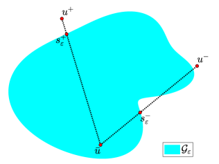
Figure 1. A possible configuration of    ${\bm{u}}$ , ${\bm{u}}^{\pm}$, and $\bm{s}^{\pm}_{\varepsilon}$ (not to scale).

Remark 2.5.

In many cases, the calculation of $\bm{s}^{\pm}_{\varepsilon}$ is cumbersome and may require a certain root-finding procedure. If the functions $\varphi_{i}({\bm{u}})$ are all concave with respect to ${\bm{u}}$, then the function $\Theta$ can be alternatively defined as

(2.15) $$\Theta(\,\hbox{\vbox{\hrule height=0.5pt\kern 1.29167pt\hbox{\kern-0.50003pt${\bm{u}}$\kern-0.50003pt}}},{\bm{u}}^{+},{\bm{u}}^{-})=\min_{i\in\mathbb{I}\cup\hat{\mathbb{I}}}\delta_{i},\quad\tilde{\varepsilon}_{i}=\begin{cases}\varepsilon_{i}&\mbox{if}~{}i\in\mathbb{I},\\ 0&\mbox{if}~{}i\in\hat{\mathbb{I}},\end{cases}$$

$$\delta_{i}=\begin{dcases}\frac{\varphi_{i}(\,\hbox{\vbox{\hrule height=0.5pt\kern 1.29167pt\hbox{\kern-0.50003pt${\bm{u}}$\kern-0.50003pt}}})-\tilde{\varepsilon}_{i}}{\varphi_{i}(\,\hbox{\vbox{\hrule height=0.5pt\kern 1.29167pt\hbox{\kern-0.50003pt${\bm{u}}$\kern-0.50003pt}}})-\min\{\varphi_{i}({\bm{u}}^{+}),\varphi_{i}({\bm{u}}^{-})\}}&\mbox{if}~{}\min\{\varphi_{i}({\bm{u}}^{+}),\varphi_{i}({\bm{u}}^{-})\}<\tilde{\varepsilon}_{i},\\ 1&\mbox{otherwise}.\end{dcases}$$

2.2.2. BP Condition #2: ${\bm{u}}^{*}_{j+\frac{1}{2}}\in{\mathcal{G}}$

We begin by proving the following two auxiliary lemmas.

Lemma 2.6.

If $\,{\bm{u}}^{-},{\bm{u}}^{+}\in{\mathcal{G}}$, $\,\hat{\sigma}^{-}\leq\sigma^{-}$, and $\,\hat{\sigma}^{+}\geq\sigma^{+}$, then

$$R_{f}(\sigma^{+},\sigma^{-},{\bm{u}}^{+},{\bm{u}}^{-})\in{\mathcal{G}}~{}\Longrightarrow~{}R_{f}(\hat{\sigma}^{+},\hat{\sigma}^{-},{\bm{u}}^{+},{\bm{u}}^{-})\in{\mathcal{G}}.$$

Proof.

We first introduce the following notation: $\varepsilon^{+}:=\hat{\sigma}^{+}-\sigma^{+}\geq 0$ and $\varepsilon^{-}:=\sigma^{-}-\hat{\sigma}^{-}\geq 0$, and then use the definition of $R_{f}$ in (2.8) to obtain

$$R_{f}(\hat{\sigma}^{+},\hat{\sigma}^{-},{\bm{u}}^{+},{\bm{u}}^{-}) =\frac{\hat{\sigma}^{+}{\bm{u}}^{+}-\hat{\sigma}^{-}{\bm{u}}^{-}-{\bm{f}}({\bm{u}}^{+})+{\bm{f}}({\bm{u}}^{-})}{\hat{\sigma}^{+}-\hat{\sigma}^{-}}$$

$$=\frac{(\sigma^{+}-\sigma^{-})\,R_{f}(\sigma^{+},\sigma^{-},{\bm{u}}^{+},{\bm{u}}^{-})+\varepsilon^{+}{\bm{u}}^{+}+\varepsilon^{-}{\bm{u}}^{-}}{\sigma^{+}-\sigma^{-}+\varepsilon^{+}+\varepsilon^{-}}.$$

This means that $R_{f}(\hat{\sigma}^{+},\hat{\sigma}^{-},{\bm{u}}^{+},{\bm{u}}^{-})$ is a convex combination of $u^{-}$, $u^{+}$, and $R_{f}(\sigma^{+},\sigma^{-},{\bm{u}}^{+},{\bm{u}}^{-})$, which implies that $R_{f}(\hat{\sigma}^{+},\hat{\sigma}^{-},{\bm{u}}^{+},{\bm{u}}^{-})\in{\mathcal{G}}$ due to the convexity of ${\mathcal{G}}$. The proof is thus completed. ∎

Lemma 2.7.

For the system (2.1) with a convex invariant region ${\mathcal{G}}$, there exist functions $\sigma^{-}({\bm{u}}^{-},{\bm{u}}^{+})$ $\leq 0$ and $\sigma^{+}({\bm{u}}^{-},{\bm{u}}^{+})\geq 0$ satisfying the following condition:

(2.16) $$R_{f}(\sigma^{+}({\bm{u}}^{-},{\bm{u}}^{+}),\sigma^{-}({\bm{u}}^{-},{\bm{u}}^{+}),{\bm{u}}^{+},{\bm{u}}^{-})\in{\mathcal{G}}~{}~{}\forall~{}{\bm{u}}^{-},{\bm{u}}^{+}\in{\mathcal{G}}.$$

Proof.

Consider the Riemann problem for the hyperbolic system (2.1) with ${\bm{u}}^{-}$ and ${\bm{u}}^{+}$ being the left and right states at $t=0$. Denote the minimum and maximum speeds of the Riemann solution by $\sigma_{\min}({\bm{u}}^{-},{\bm{u}}^{+})$ and $\sigma_{\max}({\bm{u}}^{-},{\bm{u}}^{+})$. Due to the finite speed of propagation, the Riemann fan is enclosed by the interval $[T\sigma_{\min}({\bm{u}}^{-},{\bm{u}}^{+}),T\sigma_{\max}({\bm{u}}^{-},{\bm{u}}^{+})]$ at time $t=T$. If we choose $\sigma^{+}({\bm{u}}^{-},{\bm{u}}^{+}):=\max\{\sigma_{\max}({\bm{u}}^{-},{\bm{u}}^{+}),0\}$ and $\sigma^{-}({\bm{u}}^{-},{\bm{u}}^{+}):=\min\{\sigma_{\min}({\bm{u}}^{-},{\bm{u}}^{+}),0\}$, then $R_{f}(\sigma^{+}({\bm{u}}^{-},{\bm{u}}^{+}),\sigma^{-}({\bm{u}}^{-},{\bm{u}}^{+}),{\bm{u}}^{+},{\bm{u}}^{-})$ is exactly the average of the solution of the Riemann problem at $t=T$ over the interval $[T\sigma^{-},T\sigma^{+}]$. Since the solution of the Riemann problem $u(x,T)$ is contained in the invariant region ${\mathcal{G}}$, its average over $[T\sigma^{-},T\sigma^{+}]$ is also in ${\mathcal{G}}$ due to the convexity of ${\mathcal{G}}$. Hence, the condition (2.16) is satisfied. ∎

Based on the results established in Lemmas 2.6 and 2.7, the BP Condition #2 can be enforced by a proper choice of the one-sided local speeds of propagation $\sigma^{\pm}_{j+\frac{1}{2}}$ as stated in the following theorem.

Theorem 2.8.

Given ${\bm{u}}^{\pm}_{j+\frac{1}{2}}\in{\mathcal{G}}$ for all $j$ and given functions $\sigma^{+}(\cdot,\cdot)$ and $\sigma^{-}(\cdot,\cdot)$ satisfying (2.16), the BP Condition #2 is satisfied if

$$\sigma^{+}_{j+\frac{1}{2}}\geq\sigma^{+}({\bm{u}}^{-}_{j+\frac{1}{2}},{\bm{u}}^{+}_{j+\frac{1}{2}})\quad\mbox{and}\quad\sigma^{-}_{j+\frac{1}{2}}\leq\sigma^{-}({\bm{u}}^{-}_{j+\frac{1}{2}},{\bm{u}}^{+}_{j+\frac{1}{2}})\quad\forall j.$$

Proof.

The condition (2.16) implies $R_{f}(\sigma^{+}({\bm{u}}^{-}_{j+\frac{1}{2}},{\bm{u}}^{+}_{j+\frac{1}{2}}),\sigma^{-}({\bm{u}}^{-}_{j+\frac{1}{2}},{\bm{u}}^{+}_{j+\frac{1}{2}}),{\bm{u}}^{+}_{j+\frac{1}{2}},{\bm{u}}^{-}_{j+\frac{1}{2}})\in{\mathcal{G}}$, which by Lemma 2.6 yields ${\bm{u}}^{*}_{j+\frac{1}{2}}=R_{f}(\sigma^{+}_{j+\frac{1}{2}},\sigma^{-}_{j+\frac{1}{2}},{\bm{u}}^{+}_{j+\frac{1}{2}},{\bm{u}}^{-}_{j+\frac{1}{2}})\in{\mathcal{G}}$. Hence, the BP Condition #2 is satisfied. ∎

Based on the above analysis, the task of enforcing BP Condition #2 reduces to finding suitable functions $\sigma^{-}({\bm{u}}^{-},{\bm{u}}^{+})$ and $\sigma^{+}({\bm{u}}^{-},{\bm{u}}^{+})$ satisfying (2.16). This may be not easy as it is often very difficult to exactly evaluate the minimum and maximum speeds of the Riemann solution, $\sigma_{\min}({\bm{u}}^{-},{\bm{u}}^{+})$ and $\sigma_{\max}({\bm{u}}^{-},{\bm{u}}^{+})$. Alternatively, one may estimate a lower bound $\hat{\sigma}^{-}({\bm{u}}^{-},{\bm{u}}^{+})\leq\min\{\sigma_{\min}({\bm{u}}^{-},{\bm{u}}^{+}),0\}$ and an upper bound $\hat{\sigma}^{+}({\bm{u}}^{-},{\bm{u}}^{+})\geq\max\{\sigma_{\max}({\bm{u}}^{-},{\bm{u}}^{+}),0\}$. Based on Lemma 2.6, such functions $\hat{\sigma}^{-}({\bm{u}}^{-},{\bm{u}}^{+})$ and $\hat{\sigma}^{+}({\bm{u}}^{-},{\bm{u}}^{+})$ also satisfy (2.16).

2.2.3. BP Condition #3: ${\bm{u}}^{*}_{j}\in{\mathcal{G}}$

Theorem 2.9.

Given ${\bm{u}}^{\pm}_{j+\frac{1}{2}}\in{\mathcal{G}}$ for all $j$ and given functions $\sigma^{+}(\cdot,\cdot)$ and $\sigma^{-}(\cdot,\cdot)$ satisfying (2.16), the BP Condition #3 is satisfied if

$$\sigma_{j+\frac{1}{2}}^{+}\geq\sigma^{+}({\bm{u}}^{+}_{j-\frac{1}{2}},{\bm{u}}^{-}_{j+\frac{1}{2}})\quad\mbox{and}\quad\sigma_{j-\frac{1}{2}}^{-}\leq\sigma^{-}({\bm{u}}^{+}_{j-\frac{1}{2}},{\bm{u}}^{-}_{j+\frac{1}{2}})\quad\forall j.$$

Proof.

The condition (2.16) implies $R_{f}(\sigma^{+}({\bm{u}}^{+}_{j-\frac{1}{2}},{\bm{u}}^{-}_{j+\frac{1}{2}}),\sigma^{-}({\bm{u}}^{+}_{j-\frac{1}{2}},{\bm{u}}^{-}_{j+\frac{1}{2}}),{\bm{u}}^{-}_{j+\frac{1}{2}},{\bm{u}}^{+}_{j-\frac{1}{2}})\in{\mathcal{G}}$, which by Lemma 2.6 yields

$${\bm{u}}^{*}_{j}=R_{f}(\sigma^{+}_{j+\frac{1}{2}},\sigma^{-}_{j-\frac{1}{2}},{\bm{u}}^{-}_{j+\frac{1}{2}},{\bm{u}}^{+}_{j-\frac{1}{2}})\in{\mathcal{G}}.$$

Hence, the BP Condition #3 is satisfied. ∎

According to Theorems 2.8 and 2.9, both the BP Conditions #2 and #3 can be enforced under certain conditions on the one-sided local speeds of propagation $\{\sigma_{j+\frac{1}{2}}^{\pm}\}$ as stated in the following theorem.

Theorem 2.10.

Given ${\bm{u}}^{\pm}_{j+\frac{1}{2}}\in{\mathcal{G}}$ for all $j$ and given functions $\sigma^{+}(\cdot,\cdot)$ and $\sigma^{-}(\cdot,\cdot)$ satisfying (2.16), both the BP Conditions #2 and #3 are satisfied if

$$\begin{aligned} &\sigma^{+}_{j+\frac{1}{2}}=\max\Big{\{}\sigma^{+}({\bm{u}}^{-}_{j+\frac{1}{2}},{\bm{u}}^{+}_{j+\frac{1}{2}}),\sigma^{+}({\bm{u}}^{+}_{j-\frac{1}{2}},{\bm{u}}^{-}_{j+\frac{1}{2}})\Big{\}},\\ &\sigma^{-}_{j+\frac{1}{2}}=\min\Big{\{}\sigma^{-}({\bm{u}}^{-}_{j+\frac{1}{2}},{\bm{u}}^{+}_{j+\frac{1}{2}}),\sigma^{-}({\bm{u}}^{+}_{j+\frac{1}{2}},{\bm{u}}^{-}_{j+\frac{3}{2}})\Big{\}},\end{aligned}\quad\forall j.$$

Theorem 2.10 is a direct consequence of Theorems 2.8 and 2.9, and its proof is thus omitted.

2.2.4. BP Condition #4: ${\bm{u}}^{*,\pm}_{j+\frac{1}{2}}\in{\mathcal{G}}$

Let us consider the following linear function:

(2.17) $$\bm{\psi}(\xi)={\bm{u}}^{*}_{j+\frac{1}{2}}+\frac{{\bm{d}}_{j+\frac{1}{2}}}{\sigma^{+}_{j+\frac{1}{2}}-\sigma^{-}_{j+\frac{1}{2}}}\,\xi,$$

on the interval $\xi\in\big{[}-\sigma^{+}_{j+\frac{1}{2}},-\sigma^{-}_{j+\frac{1}{2}}\big{]}$. Notice that it follows from (2.9) that $\bm{\psi}(-\sigma^{\pm}_{j+\frac{1}{2}})={\bm{u}}^{*,\pm}_{j+\frac{1}{2}}$ and thus, in order to enforce the BP Condition #4 one may use a limited modification of (2.17),

$$\widetilde{\bm{\psi}}(\xi)={\bm{u}}^{*}_{j+\frac{1}{2}}+\Theta\big{(}{\bm{u}}^{*}_{j+\frac{1}{2}},{\bm{u}}^{*,-}_{j+\frac{1}{2}},{\bm{u}}^{*,+}_{j+\frac{1}{2}}\big{)}\frac{{\bm{d}}_{j+\frac{1}{2}}}{\sigma^{+}_{j+\frac{1}{2}}-\sigma^{-}_{j+\frac{1}{2}}}\,\xi,$$

with one of the functions $\Theta$ introduced in §2.2.4 in either (2.14) or (2.15). It is easy to verify that $\tilde{\bm{u}}^{*,\pm}_{j+\frac{1}{2}}:=\widetilde{\bm{\psi}}(-\sigma^{\pm}_{j+\frac{1}{2}})\in{\mathcal{G}}$, so one has to replace the values ${\bm{u}}^{*,\pm}_{j+\frac{1}{2}}$ with their limited versions $\tilde{\bm{u}}^{*,\pm}_{j+\frac{1}{2}}$.

2.2.5. Constructing BPCU Schemes

The BPCU schemes for (2.1) can be constructed via the following steps.

Step 1. Check whether the original CU scheme satisfies the BP Condition #1. If not, modify the values ${\bm{u}}_{j+\frac{1}{2}}^{\pm}$ as described in §2.2.1.

Step 2. Check whether the modified (after Step 1) CU scheme satisfies the BP Conditions #2 and #3. If not, modify the one-sided local speeds of propagation $\sigma_{j+\frac{1}{2}}^{\pm}$ as described in §2.2.2 and §2.2.3.

Step 3. Check whether the modified (after Steps 1 and 2) CU scheme satisfies the BP Condition #4. If not, modify the “built-in” anti-diffusion term ${\bm{d}}_{j+\frac{1}{2}}$ as described in §2.2.4.

We summarize the procedure of constructing BPCU schemes in Figure 2. Following these steps, one can construct BPCU schemes for a variety of hyperbolic systems of conservation laws. In §2.3, we will construct provably BPCU schemes for the Euler equations of gas dynamics.

Figure 2. Flow chart of BPCU schemes from $\,\hbox{\vbox{\hrule height=0.5pt\kern 1.1625pt\hbox{\kern-0.45003pt${\bm{u}}$\kern-0.45003pt}}}^{\,n}_{j}$ to $\,\hbox{\vbox{\hrule height=0.5pt\kern 1.1625pt\hbox{\kern-0.45003pt${\bm{u}}$\kern-0.45003pt}}}^{\,n+1}_{j}$. To guarantee the BP property, the four formulae (blocks in yellow) may require careful redesign/verification and may differ from the counterparts of the original CU schemes.

Remark 2.11.

The BP analysis presented in §2 is based on the first-order forward Euler time discretization. The above results can be directly extended to high-order SSP Runge-Kutta or multistep method (see, e.g., [9, 10]), which can be expressed as a convex combination of forward Euler steps. The BP property of the resulting BPCU schemes remains valid thanks to the convexity of ${\mathcal{G}}$.

2.3. BPCU schemes for 1-D Euler Equations of Gas Dynamics

The 1-D Euler equations of gas dynamics for ideal gases read as (2.1) with

(2.18) $${\bm{u}}=\big{(}\rho,\rho v,E\big{)}^{\top},\quad{\bm{f}}({\bm{u}})=\big{(}\rho v,\rho v^{2}+p,(E+p)v\big{)}^{\top},\quad E=\frac{1}{2}\rho v^{2}+\frac{p}{\gamma-1}.$$

Here, $\rho$ is the density, $v$ is the velocity, $E$ is the total energy, $p$ is the pressure, and the specific heat ratio $\gamma>1$ is a constant. The speed of sound is given by $c=\sqrt{\gamma p/\rho}$, and the three eigenvalues of the Jacobian $\partial{\bm{f}}/\partial{\bm{u}}$ are $\lambda_{1}=v-c$, $\lambda_{2}=v$, and $\lambda_{3}=v+c$. A convex invariant region for the 1-D Euler equations of gas dynamics is

(2.19) $${\mathcal{G}}=\Big{\{}\,{\bm{u}}\in\mathbb{R}^{3}:\rho>0,~{}p({\bm{u}})=(\gamma-1)\Big{(}E-\frac{1}{2}\rho v^{2}\Big{)}>0\,\Big{\}}.$$

For the 1-D Euler equations of gas dynamics, the original CU schemes reviewed in §2.1 are generally not BP. In this subsection, we will use the BP framework proposed in §2.2 to modify the original CU schemes such that the BP Conditions #1–4 are satisfied, resulting in provably BPCU schemes.

2.3.1. Enforcing the BP Condition #1

We first emphasize that for the Euler equations of gas dynamics, the minmod reconstruction (2.4)–(2.5) does not, in general, satisfy the BP Condition #1. More specifically, while the positivity of density is guaranteed, the reconsructed point values of pressure may be negative. In order to address this issue, we adopt the local scaling BP limiter [50, 29] to enforce the positivity of pressure: we replace the point values ${\bm{u}}^{-}_{j+\frac{1}{2}}$ and ${\bm{u}}^{+}_{j-\frac{1}{2}}$ defined in (2.4) with

(2.20) $$\tilde{\bm{u}}^{-}_{j+\frac{1}{2}}=\,\hbox{\vbox{\hrule height=0.5pt\kern 1.29167pt\hbox{\kern-0.50003pt${\bm{u}}$\kern-0.50003pt}}}_{j}^{\,n}+\frac{\Delta x}{2}\delta_{j}\,({\bm{u}}_{x})_{j},\tilde{\bm{u}}^{+}_{j-\frac{1}{2}}=\,\hbox{\vbox{\hrule height=0.5pt\kern 1.29167pt\hbox{\kern-0.50003pt${\bm{u}}$\kern-0.50003pt}}}_{j}^{\,n}-\frac{\Delta x}{2}\delta_{j}\,({\bm{u}}_{x})_{j},~{}\delta_{j}:=\min\bigg{\{}\frac{p(\,\hbox{\vbox{\hrule height=0.5pt\kern 1.29167pt\hbox{\kern-0.50003pt${\bm{u}}$\kern-0.50003pt}}}_{j}^{\,n})-\hat{\varepsilon}_{j}}{p(\,\hbox{\vbox{\hrule height=0.5pt\kern 1.29167pt\hbox{\kern-0.50003pt${\bm{u}}$\kern-0.50003pt}}}_{j}^{\,n})-p_{j}^{\min}},1\bigg{\}},$$

$$\hat{\varepsilon}_{j}:=\min\big{\{}10^{-13},p(\,\hbox{\vbox{\hrule height=0.5pt\kern 1.29167pt\hbox{\kern-0.50003pt${\bm{u}}$\kern-0.50003pt}}}_{j}^{\,n})\big{\}},\quad p_{j}^{\min}:=\min\big{\{}p\big{(}\,{\bm{u}}^{-}_{j+\frac{1}{2}}\big{)},p\big{(}\,{\bm{u}}^{+}_{j-\frac{1}{2}}\big{)}\big{\}}.$$

Lemma 2.12.

For the 1-D Euler equations of gas dynamics (2.1), (2.18) with the invariant region (2.19), the new limited values $\tilde{\bm{u}}^{\pm}_{j+\frac{1}{2}}$ defined in (2.20) satisfy the BP Condition #1 provided $\,\hbox{\vbox{\hrule height=0.5pt\kern 1.29167pt\hbox{\kern-0.50003pt${\bm{u}}$\kern-0.50003pt}}}^{\,n}_{j}\in{\mathcal{G}}$ for all $j$.

Proof.

First, we note that since $\,\hbox{\vbox{\hrule height=0.5pt\kern 1.29167pt\hbox{\kern-0.50003pt$\rho$\kern-0.50003pt}}}^{\,n}_{j}>0$ for all $j$, the use of the minmod limiter ensures the positivity of $\rho^{\pm}_{j+\frac{1}{2}}$ for all $j$, and thus $\tilde{\rho}^{\pm}_{j+\frac{1}{2}}>0$ as $0\leq\delta_{j}\leq 1$ for all $j$. Hence, we only need to prove that $p\big{(}\tilde{\bm{u}}^{\mp}_{j\pm\frac{1}{2}}\big{)}>0$ for all $j$.

We consider two possible cases. If $p_{j}^{\min}\geq\hat{\varepsilon}_{j}$, (2.20) yields $\delta_{j}=1$ and thus $p\big{(}\tilde{\bm{u}}^{\mp}_{j\pm\frac{1}{2}}\big{)}=p\big{(}{\bm{u}}^{\mp}_{j\pm\frac{1}{2}}\big{)}\geq p_{j}^{\min}\geq\hat{\varepsilon}_{j}>0$. Otherwise, we apply Jensen’s inequality to the pressure function $p({\bm{u}})$, which is concave when $\rho>0$, and obtain

$$p\big{(}\tilde{\bm{u}}^{\mp}_{j\pm\frac{1}{2}}\big{)} =p\big{(}\,\hbox{\vbox{\hrule height=0.5pt\kern 1.29167pt\hbox{\kern-0.50003pt${\bm{u}}$\kern-0.50003pt}}}_{j}^{\,n}+\delta_{j}\big{(}{\bm{u}}^{\mp}_{j\pm\frac{1}{2}}-\,\hbox{\vbox{\hrule height=0.5pt\kern 1.29167pt\hbox{\kern-0.50003pt${\bm{u}}$\kern-0.50003pt}}}_{j}^{\,n}\big{)}\big{)}=p\big{(}(1-\delta_{j})\,\hbox{\vbox{\hrule height=0.5pt\kern 1.29167pt\hbox{\kern-0.50003pt${\bm{u}}$\kern-0.50003pt}}}_{j}^{\,n}+\delta_{j}\,{\bm{u}}^{\mp}_{j\pm\frac{1}{2}}\big{)}$$

$$\geq(1-\delta_{j})p(\,\hbox{\vbox{\hrule height=0.5pt\kern 1.29167pt\hbox{\kern-0.50003pt${\bm{u}}$\kern-0.50003pt}}}_{j}^{\,n})+\delta_{j}p\big{(}{\bm{u}}^{\mp}_{j\pm\frac{1}{2}}\big{)}$$

$$\stackrel{{\scriptstyle\eqref{23}}}{{=}}\bigg{(}1-\frac{p(\,\hbox{\vbox{\hrule height=0.5pt\kern 1.29167pt\hbox{\kern-0.50003pt${\bm{u}}$\kern-0.50003pt}}}_{j}^{\,n})-\hat{\varepsilon}_{j}}{p(\,\hbox{\vbox{\hrule height=0.5pt\kern 1.29167pt\hbox{\kern-0.50003pt${\bm{u}}$\kern-0.50003pt}}}_{j}^{\,n})-p_{j}^{\min}}\bigg{)}p(\,\hbox{\vbox{\hrule height=0.5pt\kern 1.29167pt\hbox{\kern-0.50003pt${\bm{u}}$\kern-0.50003pt}}}_{j}^{\,n})+\frac{p(\,\hbox{\vbox{\hrule height=0.5pt\kern 1.29167pt\hbox{\kern-0.50003pt${\bm{u}}$\kern-0.50003pt}}}_{j}^{\,n})-\hat{\varepsilon}_{j}}{p(\,\hbox{\vbox{\hrule height=0.5pt\kern 1.29167pt\hbox{\kern-0.50003pt${\bm{u}}$\kern-0.50003pt}}}_{j}^{\,n})-p_{j}^{\min}}\,p\big{(}{\bm{u}}^{\mp}_{j\pm\frac{1}{2}}\big{)}$$

$$\geq\frac{\hat{\varepsilon}_{j}-p_{j}^{\min}}{p(\,\hbox{\vbox{\hrule height=0.5pt\kern 1.29167pt\hbox{\kern-0.50003pt${\bm{u}}$\kern-0.50003pt}}}_{j}^{\,n})-p_{j}^{\min}}\,p(\,\hbox{\vbox{\hrule height=0.5pt\kern 1.29167pt\hbox{\kern-0.50003pt${\bm{u}}$\kern-0.50003pt}}}_{j}^{\,n})+\frac{p(\,\hbox{\vbox{\hrule height=0.5pt\kern 1.29167pt\hbox{\kern-0.50003pt${\bm{u}}$\kern-0.50003pt}}}_{j}^{\,n})-\hat{\varepsilon}_{j}}{p(\,\hbox{\vbox{\hrule height=0.5pt\kern 1.29167pt\hbox{\kern-0.50003pt${\bm{u}}$\kern-0.50003pt}}}_{j}^{\,n})-p_{j}^{\min}}\,p_{j}^{\min}=\hat{\varepsilon}_{j}>0.$$

The proof is completed. ∎

2.3.2. The BP Conditions #2 and #3

Equipped with the reconstructed point values ${\bm{u}}^{\pm}_{j+\frac{1}{2}}=\big{(}\rho^{\pm}_{j+\frac{1}{2}},(\rho v)^{\pm}_{j+\frac{1}{2}},E^{\pm}_{j+\frac{1}{2}}\big{)}^{\top}$, we compute the one-sided local speeds of propagation using equation (2.6), which for the Euler equations of gas dynamics reads as

(2.21) $$\sigma^{-}_{j+\frac{1}{2}}=\min\big{\{}v^{-}_{j+\frac{1}{2}}-c^{-}_{j+\frac{1}{2}},v^{+}_{j+\frac{1}{2}}-c^{+}_{j+\frac{1}{2}},0\big{\}},~{}~{}\sigma^{+}_{j+\frac{1}{2}}=\max\big{\{}v^{-}_{j+\frac{1}{2}}+c^{-}_{j+\frac{1}{2}},v^{+}_{j+\frac{1}{2}}+c^{+}_{j+\frac{1}{2}},0\big{\}},$$

where $v^{\pm}_{j+\frac{1}{2}}=(\rho v)^{\pm}_{j+\frac{1}{2}}/\rho^{\pm}_{j+\frac{1}{2}}$, $c^{\pm}_{j+\frac{1}{2}}=\sqrt{\gamma p^{\pm}_{j+\frac{1}{2}}/\rho^{\pm}_{j+\frac{1}{2}}}$, and $p^{\pm}_{j+\frac{1}{2}}=p\big{(}{\bm{u}}^{\pm}_{j+\frac{1}{2}}\big{)}$. In fact, $\sigma^{\pm}_{j+\frac{1}{2}}$ defined in (2.21) and corrected according to Remark 2.1, satisfy both the BP Conditions #2 and #3. In order to prove this, we adopt the GQL approach [34].

First, recall that according to [34, Theorem 5.1], the equivalent GQL representation of the invariant region (2.19) is given by

$${\mathcal{G}}_{*}:=\left\{\,{\bm{u}}\in\mathbb{R}^{3}:{\bm{u}}\cdot\bm{e}_{1}>0,\,{\bm{u}}_{1}\cdot\bm{n}_{*}>0~{}\forall v_{*}\in\mathbb{R}\,\right\},$$

where $\bm{e}_{1}=(1,0,0)^{\top}$ and $\bm{n}_{*}=\big{(}\frac{v_{*}^{2}}{2},-v_{*},1\big{)}^{\top}$.

We then prove the following two auxiliary lemmas.

Lemma 2.13.

For any ${\bm{u}}\in{\mathcal{G}}$, we have $\left[c{\bm{u}}\pm\big{(}v{\bm{u}}-\bm{f}({\bm{u}})\big{)}\right]\cdot\bm{n}>0$, where $\bm{n}=\bm{e}_{1}$ or $\bm{n}=\bm{n}_{*}$ for any $v_{*}\in\mathbb{R}$.

Proof.

If $\bm{n}=\bm{e}_{1}$, then $\left[c{\bm{u}}\pm\big{(}v{\bm{u}}-\bm{f}({\bm{u}})\big{)}\right]\cdot\bm{e}_{1}=c\rho>0$. If $\bm{n}=\bm{n}_{*}$, then

$$c\,{\bm{u}}\cdot\bm{n}_{*}=\sqrt{\frac{\gamma p}{\rho}}\left(\frac{\rho}{2}(v-v_{*})^{2}+\frac{p}{\gamma-1}\right)>\sqrt{\frac{(\gamma-1)p}{2\rho}}\sqrt{2\rho(v-v_{*})^{2}\frac{p}{\gamma-1}}=p\,|v-v_{*}|,$$

which implies

$$\left[c{\bm{u}}\pm\big{(}v{\bm{u}}-\bm{f}({\bm{u}})\big{)}\right]\cdot\bm{n}_{*}>p\,|v-v_{*}|\mp(0,p,pv)^{\top}\cdot\bm{n}_{*}=p\,|v-v_{*}|\mp p(v-v_{*})\geq 0~{}~{}\forall v_{*}\in\mathbb{R}.$$

The proof is completed. ∎

Lemma 2.14.

For any ${\bm{u}}^{+},{\bm{u}}^{-}\in{\mathcal{G}}$, if $\sigma^{+}\geq v^{+}+c^{+}$, $\sigma^{-}\leq v^{-}-c^{-}$, and $\sigma^{+}>\sigma^{-}$, then $R_{f}(\sigma^{+},\sigma^{-},{\bm{u}}^{+},{\bm{u}}^{-})\in{\mathcal{G}}$.

Proof.

For $\bm{n}=\bm{e}_{1}$ or $\bm{n}=\bm{n}_{*}$, [34, Theorem 5.1] yields ${\bm{u}}^{+}\cdot\bm{n}>0$ and ${\bm{u}}^{-}\cdot\bm{n}>0$. Lemma 2.13 yields

$$\left[\sigma^{+}{\bm{u}}^{+}-\bm{f}({\bm{u}}^{+})\right]\cdot\bm{n} =\left[(v^{+}+c^{+})\,{\bm{u}}^{+}-\bm{f}({\bm{u}}^{+})\right]\cdot\bm{n}+\left[\sigma^{+}-(v^{+}+c^{+})\right]({\bm{u}}^{+}\cdot\bm{n})$$

$$\geq\left[c^{+}{\bm{u}}^{+}+\left(v^{+}{\bm{u}}^{+}-\bm{f}({\bm{u}}^{+})\right)\right]\cdot\bm{n}>0,$$

$$\left[\bm{f}({\bm{u}}^{-})-\sigma^{-}{\bm{u}}^{-}\right]\cdot\bm{n} =\left[\bm{f}({\bm{u}}^{-})-(v^{-}-c^{-})\,{\bm{u}}^{-}\right]\cdot\bm{n}+\left[(v^{-}-c^{+})-\sigma^{-}\right]({\bm{u}}^{-}\cdot\bm{n})$$

$$\geq\left[c^{-}{\bm{u}}^{-}-\left(v^{-}{\bm{u}}^{-}-\bm{f}({\bm{u}}^{-})\right)\right]\cdot\bm{n}>0.$$

Therefore,

$$R_{f}(\sigma^{+},\sigma^{-},{\bm{u}}^{+},{\bm{u}}^{-})\cdot\bm{n}\stackrel{{\scriptstyle\eqref{8}}}{{=}}\frac{\left[\bm{f}({\bm{u}}^{-})-\sigma^{-}{\bm{u}}^{-}\right]\cdot\bm{n}+\left[\sigma^{+}{\bm{u}}^{+}-\bm{f}({\bm{u}}^{+})\right]\cdot\bm{n}}{\sigma^{+}-\sigma^{-}}>0.$$

Hence, according to [34, Theorem 5.1], $R_{f}(\sigma^{+},\sigma^{-},{\bm{u}}^{+},{\bm{u}}^{-})\in{\mathcal{G}}_{*}={\mathcal{G}}$, and the proof is completed. ∎

We now state and prove the main result of this subsection.

Lemma 2.15.

For the 1-D Euler equations of gas dynamics (2.1), (2.18) with the invariant region (2.19), the speeds $\sigma^{\pm}_{j+\frac{1}{2}}$ defined in (2.21) and corrected according to Remark 2.1, satisfy both the BP Conditions #2 and #3.

Proof.

We note that (2.21) together with the correction introduced in Remark 2.1 imply $\,\sigma^{+}_{j+\frac{1}{2}}\geq v^{+}_{j+\frac{1}{2}}+c^{+}_{j+\frac{1}{2}}$, $\,\sigma^{-}_{j+\frac{1}{2}}\leq v^{-}_{j+\frac{1}{2}}-c^{-}_{j+\frac{1}{2}}$, and $\,\sigma^{+}_{j+\frac{1}{2}}>\sigma^{-}_{j+\frac{1}{2}}$, and then we use Lemma 2.14 to obtain ${\bm{u}}^{*}_{j+\frac{1}{2}}=R_{f}\big{(}\sigma^{+}_{j+\frac{1}{2}},\sigma^{-}_{j+\frac{1}{2}},{\bm{u}}^{+}_{j+\frac{1}{2}},{\bm{u}}^{-}_{j+\frac{1}{2}}\big{)}\in{\mathcal{G}}$, which means that the BP Condition #2 is satisfied. Similarly, because $\,\sigma^{+}_{j+\frac{1}{2}}\geq v^{-}_{j+\frac{1}{2}}+c^{-}_{j+\frac{1}{2}}$, $\,\sigma^{-}_{j-\frac{1}{2}}\leq v^{+}_{j-\frac{1}{2}}-c^{+}_{j-\frac{1}{2}}$, and $\,\sigma^{+}_{j+\frac{1}{2}}>\sigma^{-}_{j-\frac{1}{2}}$, Lemma 2.14 yields
${\bm{u}}^{*}_{j}=R_{f}\big{(}\sigma^{+}_{j+\frac{1}{2}},\sigma^{-}_{j-\frac{1}{2}},{\bm{u}}^{-}_{j+\frac{1}{2}},{\bm{u}}^{+}_{j-\frac{1}{2}}\big{)}\in{\mathcal{G}}$, so that the BP Condition #3 is satisfied. The proof is thus completed. ∎

2.3.3. Enforcing the BP Condition #4

Our numerical experiments (not shown in this paper) clearly demonstrate that for the Euler equations of gas dynamics, the use of the anti-diffusion (2.7) may lead to appearance of negative pressures. In order to address this issue, we replace the anti-diffusion term ${\bm{d}}_{j+\frac{1}{2}}$ with

(2.22) $$\widetilde{\bm{d}}_{j+\frac{1}{2}}=\beta_{j+\frac{1}{2}}{\bm{d}}_{j+\frac{1}{2}}=\beta_{j+\frac{1}{2}}\,{\rm minmod}\,\big{(}{\bm{u}}^{+}_{j+\frac{1}{2}}-{\bm{u}}^{*}_{j+\frac{1}{2}},{\bm{u}}^{*}_{j+\frac{1}{2}}-{\bm{u}}^{-}_{j+\frac{1}{2}}\big{)},$$

$$\beta_{j+\frac{1}{2}}:=\min\bigg{\{}\frac{p\big{(}{\bm{u}}^{*}_{j+\frac{1}{2}}\big{)}-\hat{\varepsilon}_{j+\frac{1}{2}}}{p\big{(}{\bm{u}}^{*}_{j+\frac{1}{2}}\big{)}-p_{j+\frac{1}{2}}^{\min}},1\bigg{\}},$$

$$\hat{\varepsilon}_{j+\frac{1}{2}}:=\min\big{\{}10^{-13},p\big{(}{\bm{u}}^{*}_{j+\frac{1}{2}}\big{)}\big{\}},\quad p_{j+\frac{1}{2}}^{\min}:=\min\big{\{}p\big{(}{\bm{u}}^{*,+}_{j+\frac{1}{2}}\big{)},p\big{(}{\bm{u}}^{*,-}_{j+\frac{1}{2}}\big{)}\big{\}},$$

where ${\bm{u}}^{*,\pm}_{j+\frac{1}{2}}$ are defined in (2.9).

Lemma 2.16.

For the 1-D Euler equations of gas dynamics (2.1), (2.18) with the invariant region (2.19), the modified quantity

$$\tilde{\bm{u}}^{*,\pm}_{j+\frac{1}{2}}:={\bm{u}}^{*}_{j+\frac{1}{2}}-\frac{\sigma^{\pm}_{j+\frac{1}{2}}}{\sigma^{+}_{j+\frac{1}{2}}-\sigma^{-}_{j+\frac{1}{2}}}\widetilde{\bm{d}}_{j+\frac{1}{2}}$$

satisfies the BP Conditions #4.

Proof.

First, we use (2.22) and (2.9) to rewrite $\tilde{\bm{u}}^{*,\pm}_{j+\frac{1}{2}}$ as

$$\tilde{\bm{u}}^{*,\pm}_{j+\frac{1}{2}} ={\bm{u}}^{*}_{j+\frac{1}{2}}-\beta_{j+\frac{1}{2}}\frac{\sigma^{\pm}_{j+\frac{1}{2}}}{\sigma^{+}_{j+\frac{1}{2}}-\sigma^{-}_{j+\frac{1}{2}}}\,{\rm minmod}\,\big{(}{\bm{u}}^{+}_{j+\frac{1}{2}}-{\bm{u}}^{*}_{j+\frac{1}{2}},{\bm{u}}^{*}_{j+\frac{1}{2}}-{\bm{u}}^{-}_{j+\frac{1}{2}}\big{)}$$

$$={\bm{u}}^{*}_{j+\frac{1}{2}}-\beta_{j+\frac{1}{2}}\big{(}{\bm{u}}^{*}_{j+\frac{1}{2}}-{\bm{u}}^{*,\pm}_{j+\frac{1}{2}}\big{)}=\big{(}1-\beta_{j+\frac{1}{2}}\big{)}{\bm{u}}^{*}_{j+\frac{1}{2}}+\beta_{j+\frac{1}{2}}{\bm{u}}^{*,\pm}_{j+\frac{1}{2}}.$$

Since $\rho^{\pm}_{j+\frac{1}{2}}>0$ and $\rho^{*}_{j+\frac{1}{2}}>0$, in order to show that $\tilde{\rho}^{*,\pm}_{j+\frac{1}{2}}>0$, one has to show that $\rho^{*,\pm}_{j+\frac{1}{2}}>0$. Indeed, if $\rho^{+}_{j+\frac{1}{2}}>\rho^{*}_{j+\frac{1}{2}}>\rho^{-}_{j+\frac{1}{2}}$, then

$$\rho^{*,+}_{j+\frac{1}{2}} =\rho^{*}_{j+\frac{1}{2}}-\frac{\sigma^{+}_{j+\frac{1}{2}}}{\sigma^{+}_{j+\frac{1}{2}}-\sigma^{-}_{j+\frac{1}{2}}}\,{\rm minmod}\,\big{(}\rho^{+}_{j+\frac{1}{2}}-\rho^{*}_{j+\frac{1}{2}},\rho^{*}_{j+\frac{1}{2}}-\rho^{-}_{j+\frac{1}{2}}\big{)}\geq\rho^{*}_{j+\frac{1}{2}}-\big{(}\rho^{*}_{j+\frac{1}{2}}-\rho^{-}_{j+\frac{1}{2}}\big{)}=\rho^{-}_{j+\frac{1}{2}}>0,$$

and otherwise, $\rho^{*,+}_{j+\frac{1}{2}}=\rho^{*}_{j+\frac{1}{2}}>0$. Similarly, if $\rho^{+}_{j+\frac{1}{2}}<\rho^{*}_{j+\frac{1}{2}}<\rho^{-}_{j+\frac{1}{2}}$, then

$$\rho^{*,-}_{j+\frac{1}{2}} =\rho^{*}_{j+\frac{1}{2}}-\frac{\sigma^{-}_{j+\frac{1}{2}}}{\sigma^{+}_{j+\frac{1}{2}}-\sigma^{-}_{j+\frac{1}{2}}}\,{\rm minmod}\,\big{(}\rho^{+}_{j+\frac{1}{2}}-\rho^{*}_{j+\frac{1}{2}},\rho^{*}_{j+\frac{1}{2}}-\rho^{-}_{j+\frac{1}{2}}\big{)}\geq\rho^{*}_{j+\frac{1}{2}}+\big{(}\rho^{+}_{j+\frac{1}{2}}-\rho^{*}_{j+\frac{1}{2}}\big{)}=\rho^{+}_{j+\frac{1}{2}}>0,$$

and otherwise, $\rho^{*,-}_{j+\frac{1}{2}}=\rho^{*}_{j+\frac{1}{2}}>0$.

In order to prove that $p\big{(}\tilde{\bm{u}}^{*,\pm}_{j+\frac{1}{2}}\big{)}>0$, we consider two possible cases. If $p_{j+\frac{1}{2}}^{\min}\geq\hat{\varepsilon}_{j+\frac{1}{2}}$, (2.22) yields $\beta_{j+\frac{1}{2}}=1$ and thus $p\big{(}\tilde{\bm{u}}^{*,\pm}_{j+\frac{1}{2}}\big{)}=p\big{(}{\bm{u}}^{*,\pm}_{j+\frac{1}{2}}\big{)}\geq p_{j+\frac{1}{2}}^{\min}\geq\hat{\varepsilon}_{j}>0$. Otherwise, we apply Jensen’s inequality to the pressure function $p({\bm{u}})$, which is concave when $\rho>0$, and obtain

$$p\big{(}\tilde{\bm{u}}^{*,\pm}_{j+\frac{1}{2}}\big{)} =p\big{(}\big{(}1-\beta_{j+\frac{1}{2}}\big{)}\,{\bm{u}}_{j+\frac{1}{2}}^{*}+\beta_{j+\frac{1}{2}}{\bm{u}}^{*,\pm}_{j+\frac{1}{2}}\big{)}\geq(1-\beta_{j+\frac{1}{2}})p\big{(}{\bm{u}}_{j+\frac{1}{2}}^{*}\big{)}+\beta_{j+\frac{1}{2}}p\big{(}{\bm{u}}^{*,\pm}_{j+\frac{1}{2}}\big{)}$$

$$\stackrel{{\scriptstyle\eqref{26}}}{{=}}\bigg{(}1-\frac{p\big{(}{\bm{u}}^{*}_{j+\frac{1}{2}}\big{)}-\hat{\varepsilon}_{j+\frac{1}{2}}}{p\big{(}{\bm{u}}^{*}_{j+\frac{1}{2}}\big{)}-p_{j+\frac{1}{2}}^{\min}}\bigg{)}p\big{(}{\bm{u}}_{j+\frac{1}{2}}^{*}\big{)}+\frac{p\big{(}{\bm{u}}^{*}_{j+\frac{1}{2}}\big{)}-\hat{\varepsilon}_{j+\frac{1}{2}}}{p\big{(}{\bm{u}}^{*}_{j+\frac{1}{2}}\big{)}-p_{j+\frac{1}{2}}^{\min}}\,p\big{(}{\bm{u}}^{*,\pm}_{j+\frac{1}{2}}\big{)}$$

$$\geq\frac{\hat{\varepsilon}_{j+\frac{1}{2}}-p_{j+\frac{1}{2}}^{\min}}{p\big{(}{\bm{u}}^{*}_{j+\frac{1}{2}}\big{)}-p_{j+\frac{1}{2}}^{\min}}\,p\big{(}{\bm{u}}_{j+\frac{1}{2}}^{*}\big{)}+\frac{p\big{(}{\bm{u}}^{*}_{j+\frac{1}{2}}\big{)}-\hat{\varepsilon}_{j+\frac{1}{2}}}{p\big{(}{\bm{u}}^{*}_{j+\frac{1}{2}}\big{)}-p_{j+\frac{1}{2}}^{\min}}\,p_{j+\frac{1}{2}}^{\min}=\hat{\varepsilon}_{j+\frac{1}{2}}>0.$$

The proof is completed. ∎

2.3.4. Constructing BPCU Schemes

Based on Lemmas 2.12, 2.15 and 2.16, the BPCU schemes for the 1-D Euler equations of gas dynamics (2.1), (2.18) can be constructed via the following steps.

Step 1. Modify the reconstructed point values ${\bm{u}}_{j+\frac{1}{2}}^{\pm}$ using (2.20).

Step 2. Modify the “built-in” anti-diffusion term ${\bm{d}}_{j+\frac{1}{2}}$ using (2.22).

3. Two-Dimensional BPCU Schemes

The 1-D BP framework for CU schemes proposed in §2.2 can be extended to multiple dimensions. Without loss of generality, we present the 2-D BP framework and 2-D BPCU schemes, while the extensions to higher dimensions are similar and thus omitted.

Consider the 2-D hyperbolic system of conservation laws

(3.1) $${\bm{u}}_{t}+{\bm{f}}({\bm{u}})_{x}+{\bm{g}}({\bm{u}})_{y}=\bm{0}.$$

Assume that the computational mesh is uniform with Cartesian cells $\Omega_{j,k}=[x_{j-\frac{1}{2}},x_{j+\frac{1}{2}}]\times[y_{k-\frac{1}{2}},y_{k+\frac{1}{2}}]$. Let $\,\hbox{\vbox{\hrule height=0.5pt\kern 1.29167pt\hbox{\kern-0.50003pt${\bm{u}}$\kern-0.50003pt}}}_{j,k}^{\,n}$ be the approximation of the cell average of ${\bm{u}}(x,y,t^{n})$ over $\Omega_{j,k}$ at time $t=t^{n}$. For the sake of convenience, we focus on the first-order forward Euler time discretization, while all of the results below are also applicable to higher-order SSP time discretization.

The 2-D CU schemes read as

(3.2) $$\hbox{\vbox{\hrule height=0.5pt\kern 1.29167pt\hbox{\kern-0.50003pt${\bm{u}}$\kern-0.50003pt}}}^{\,n+1}_{j,k}=\,\hbox{\vbox{\hrule height=0.5pt\kern 1.29167pt\hbox{\kern-0.50003pt${\bm{u}}$\kern-0.50003pt}}}^{\,n}_{j,k}-\lambda^{n}\left(\hat{\bm{f}}_{j+\frac{1}{2},k}-\hat{\bm{f}}_{j-\frac{1}{2},k}\right)-\mu^{n}\left(\hat{\bm{g}}_{j,k+\frac{1}{2}}-\hat{\bm{g}}_{j,k-\frac{1}{2}}\right),\quad\mu^{n}:=\frac{\Delta t^{n}}{\Delta y},$$

with $\lambda^{n}$ and $\Delta t^{n}$ given by (2.2) and the CU numerical fluxes

(3.3) $$\hat{\bm{f}}_{j+\frac{1}{2},k} =\frac{\sigma^{+}_{j+\frac{1}{2},k}{\bm{f}}\big{(}{\bm{u}}^{-}_{j+\frac{1}{2},k}\big{)}-\sigma^{-}_{j+\frac{1}{2},k}{\bm{f}}\big{(}{\bm{u}}^{+}_{j+\frac{1}{2},k}\big{)}}{\sigma^{+}_{j+\frac{1}{2},k}-\sigma^{-}_{j+\frac{1}{2},k}}+\frac{\sigma^{+}_{j+\frac{1}{2},k}\sigma^{-}_{j+\frac{1}{2},k}}{\sigma^{+}_{j+\frac{1}{2},k}-\sigma^{-}_{j+\frac{1}{2},k}}\big{(}{\bm{u}}^{+}_{j+\frac{1}{2},k}-{\bm{u}}^{-}_{j+\frac{1}{2},k}-{\bm{d}}_{j+\frac{1}{2},k}\big{)},$$

$$\hat{\bm{g}}_{j,k+\frac{1}{2}} =\frac{\sigma^{+}_{j,k+\frac{1}{2}}{\bm{g}}\big{(}{\bm{u}}^{-}_{j,k+\frac{1}{2}}\big{)}-\sigma^{-}_{j,k+\frac{1}{2}}{\bm{g}}\big{(}{\bm{u}}^{+}_{j,k+\frac{1}{2}}\big{)}}{\sigma^{+}_{j,k+\frac{1}{2}}-\sigma^{-}_{j,k+\frac{1}{2}}}+\frac{\sigma^{+}_{j,k+\frac{1}{2}}\sigma^{-}_{j,k+\frac{1}{2}}}{\sigma^{+}_{j,k+\frac{1}{2}}-\sigma^{-}_{j,k+\frac{1}{2}}}\big{(}{\bm{u}}^{+}_{j,k+\frac{1}{2}}-{\bm{u}}^{-}_{j,k+\frac{1}{2}}-{\bm{d}}_{j,k+\frac{1}{2}}\big{)}.$$

In (3.3), ${\bm{u}}^{\pm}_{j+\frac{1}{2},k}$ and ${\bm{u}}^{\pm}_{j,k+\frac{1}{2}}$ are the one-sided values of the reconstructed solution at the midpoints of the cell interfaces $(x,y)=(x_{j+\frac{1}{2}},y_{k})$ and $(x,y)=(x_{j},y_{k+\frac{1}{2}})$, respectively:

(3.4) $${\bm{u}}^{-}_{j+\frac{1}{2},k}=\,\hbox{\vbox{\hrule height=0.5pt\kern 1.29167pt\hbox{\kern-0.50003pt${\bm{u}}$\kern-0.50003pt}}}_{j,k}^{\,n}+\frac{\Delta x}{2}({\bm{u}}_{x})_{j,k}^{n},~{}~{}{\bm{u}}^{+}_{j+\frac{1}{2},k}=\,\hbox{\vbox{\hrule height=0.5pt\kern 1.29167pt\hbox{\kern-0.50003pt${\bm{u}}$\kern-0.50003pt}}}_{j+1,k}^{\,n}-\frac{\Delta x}{2}({\bm{u}}_{x})_{j+1,k}^{n},$$

$${\bm{u}}^{-}_{j,k+\frac{1}{2}}=\,\hbox{\vbox{\hrule height=0.5pt\kern 1.29167pt\hbox{\kern-0.50003pt${\bm{u}}$\kern-0.50003pt}}}_{j,k}^{\,n}+\frac{\Delta y}{2}({\bm{u}}_{y})_{j,k}^{n},~{}~{}{\bm{u}}^{+}_{j,k+\frac{1}{2}}=\,\hbox{\vbox{\hrule height=0.5pt\kern 1.29167pt\hbox{\kern-0.50003pt${\bm{u}}$\kern-0.50003pt}}}_{j+1,k}^{\,n}-\frac{\Delta y}{2}({\bm{u}}_{y})_{j,k+1}^{n},$$

where

(3.5) $$\begin{aligned} &({\bm{u}}_{x})_{j,k}^{n}={\rm minmod}\left(\theta\,\frac{\hbox{\vbox{\hrule height=0.5pt\kern 1.29167pt\hbox{\kern-0.50003pt${\bm{u}}$\kern-0.50003pt}}}_{j,k}^{\,n}-\,\hbox{\vbox{\hrule height=0.5pt\kern 1.29167pt\hbox{\kern-0.50003pt${\bm{u}}$\kern-0.50003pt}}}_{j-1,k}^{\,n}}{\Delta x},\frac{\hbox{\vbox{\hrule height=0.5pt\kern 1.29167pt\hbox{\kern-0.50003pt${\bm{u}}$\kern-0.50003pt}}}_{j+1,k}^{\,n}-\,\hbox{\vbox{\hrule height=0.5pt\kern 1.29167pt\hbox{\kern-0.50003pt${\bm{u}}$\kern-0.50003pt}}}_{j-1,k}^{\,n}}{2\Delta x},\theta\,\frac{\hbox{\vbox{\hrule height=0.5pt\kern 1.29167pt\hbox{\kern-0.50003pt${\bm{u}}$\kern-0.50003pt}}}_{j+1,k}^{\,n}-\,\hbox{\vbox{\hrule height=0.5pt\kern 1.29167pt\hbox{\kern-0.50003pt${\bm{u}}$\kern-0.50003pt}}}_{j,k}^{\,n}}{\Delta x}\right),\\ &({\bm{u}}_{y})_{j,k}^{n}={\rm minmod}\left(\theta\,\frac{\hbox{\vbox{\hrule height=0.5pt\kern 1.29167pt\hbox{\kern-0.50003pt${\bm{u}}$\kern-0.50003pt}}}_{j,k}^{\,n}-\,\hbox{\vbox{\hrule height=0.5pt\kern 1.29167pt\hbox{\kern-0.50003pt${\bm{u}}$\kern-0.50003pt}}}_{j,k-1}^{\,n}}{\Delta y},\frac{\hbox{\vbox{\hrule height=0.5pt\kern 1.29167pt\hbox{\kern-0.50003pt${\bm{u}}$\kern-0.50003pt}}}_{j,k+1}^{\,n}-\,\hbox{\vbox{\hrule height=0.5pt\kern 1.29167pt\hbox{\kern-0.50003pt${\bm{u}}$\kern-0.50003pt}}}_{j,k-1}^{\,n}}{2\Delta y},\theta\,\frac{\hbox{\vbox{\hrule height=0.5pt\kern 1.29167pt\hbox{\kern-0.50003pt${\bm{u}}$\kern-0.50003pt}}}_{j,k+1}^{\,n}-\,\hbox{\vbox{\hrule height=0.5pt\kern 1.29167pt\hbox{\kern-0.50003pt${\bm{u}}$\kern-0.50003pt}}}_{j,k}^{\,n}}{\Delta y}\right),\end{aligned}\quad\theta\in[1,2].$$

The quantities $\sigma^{\pm}_{j+\frac{1}{2},k}$ and $\sigma^{\pm}_{j,k+\frac{1}{2}}$ in (3.3) denote the one-sided local speeds of propagation in the $x$- and $y$-directions, respectively, and they can be estimated using the smallest and largest eigenvalues of the Jacobians $A({\bm{u}}):=\partial{\bm{f}}/\partial{\bm{u}}$ and $B({\bm{u}}):=\partial{\bm{g}}/\partial{\bm{u}}$:

(3.6) $$\sigma^{-}_{j+\frac{1}{2},k} =\min\big{\{}\lambda_{1}\big{(}A\big{(}{\bm{u}}^{-}_{j+\frac{1}{2},k}\big{)}\big{)},\lambda_{1}\big{(}A\big{(}{\bm{u}}^{+}_{j+\frac{1}{2},k}\big{)}\big{)},0\big{\}},$$

$$\sigma^{+}_{j+\frac{1}{2},k} =\max\big{\{}\lambda_{m}\big{(}A\big{(}{\bm{u}}^{-}_{j+\frac{1}{2},k}\big{)}\big{)},\lambda_{m}\big{(}A\big{(}{\bm{u}}^{+}_{j+\frac{1}{2},k}\big{)}\big{)},0\big{\}},$$

$$\sigma^{-}_{j,k+\frac{1}{2}} =\min\big{\{}\lambda_{1}\big{(}B\big{(}{\bm{u}}^{-}_{j,k+\frac{1}{2}}\big{)}\big{)},\lambda_{1}\big{(}B\big{(}{\bm{u}}^{+}_{j,k+\frac{1}{2}}\big{)}\big{)},0\big{\}},$$

$$\sigma^{+}_{j,k+\frac{1}{2}} =\max\big{\{}\lambda_{m}\big{(}B\big{(}{\bm{u}}^{-}_{j,k+\frac{1}{2}}\big{)}\big{)},\lambda_{m}\big{(}B\big{(}{\bm{u}}^{+}_{j,k+\frac{1}{2}}\big{)}\big{)},0\big{\}}.$$

As in the 1-D case, (3.6) should be modified as in 2.1 to desingularize the computations in (3.3).

Finally, ${\bm{d}}_{j+\frac{1}{2},k}$ and ${\bm{d}}_{j,k+\frac{1}{2}}$ in (3.3) are the “built-in” anti-diffusion terms given by (see [4])

(3.7) $${\bm{d}}_{j+\frac{1}{2},k}={\rm minmod}\,\big{(}{\bm{u}}^{+}_{j+\frac{1}{2},k}-{\bm{u}}^{*}_{j+\frac{1}{2},k},{\bm{u}}^{*}_{j+\frac{1}{2},k}-{\bm{u}}^{-}_{j+\frac{1}{2},k}\big{)},$$

$${\bm{d}}_{j,k+\frac{1}{2}}={\rm minmod}\,\big{(}{\bm{u}}^{+}_{j,k+\frac{1}{2}}-{\bm{u}}^{*}_{j,k+\frac{1}{2}},{\bm{u}}^{*}_{j,k+\frac{1}{2}}-{\bm{u}}^{-}_{j,k+\frac{1}{2}}\big{)},$$

where

(3.8) $${\bm{u}}^{*}_{j+\frac{1}{2},k}=R_{f}\big{(}\sigma^{+}_{j+\frac{1}{2},k},\sigma^{-}_{j+\frac{1}{2},k},{\bm{u}}^{+}_{j+\frac{1}{2},k},{\bm{u}}^{-}_{j+\frac{1}{2},k}\big{)},$$

$$R_{f}(\sigma^{+},\sigma^{-},{\bm{u}}^{+},{\bm{u}}^{-}):=\frac{\sigma^{+}{\bm{u}}^{+}-\sigma^{-}{\bm{u}}^{-}-{\bm{f}}({\bm{u}}^{+})+{\bm{f}}({\bm{u}}^{-})}{\sigma^{+}-\sigma^{-}},$$

$${\bm{u}}^{*}_{j,k+\frac{1}{2}}=R_{g}\big{(}\sigma^{+}_{j,k+\frac{1}{2}},\sigma^{-}_{j,k+\frac{1}{2}},{\bm{u}}^{+}_{j,k+\frac{1}{2}},{\bm{u}}^{-}_{j,k+\frac{1}{2}}\big{)},$$

$$R_{g}(\sigma^{+},\sigma^{-},{\bm{u}}^{+},{\bm{u}}^{-}):=\frac{\sigma^{+}{\bm{u}}^{+}-\sigma^{-}{\bm{u}}^{-}-{\bm{g}}({\bm{u}}^{+})+{\bm{g}}({\bm{u}}^{-})}{\sigma^{+}-\sigma^{-}}.$$

The CU scheme (3.2)–(3.8) is, in general, not BP. In order to design a BPCU scheme, one may need to properly modify the reconstructed point values (${\bm{u}}_{j+\frac{1}{2},k}^{\pm}$ and ${\bm{u}}_{j,k+\frac{1}{2}}^{\pm}$), one-sided local speeds of propagation ($\sigma_{j+\frac{1}{2},k}^{\pm}$ and $\sigma_{j,k+\frac{1}{2}}^{\pm}$), and “built-in” anti-diffusion terms (${\bm{d}}_{j+\frac{1}{2},k}$ and ${\bm{d}}_{j,k+\frac{1}{2}}$). To this end, we first introduce the following auxiliary quantities:

(3.9) $${\bm{u}}^{*,\pm}_{j+\frac{1}{2},k}:={\bm{u}}^{*}_{j+\frac{1}{2},k}-\frac{\sigma^{\pm}_{j+\frac{1}{2},k}}{\sigma^{+}_{j+\frac{1}{2},k}-\sigma^{-}_{j+\frac{1}{2},k}}\,{\bm{d}}_{j+\frac{1}{2},k},$$

$${\bm{u}}^{*,x}_{j,k}:=R_{f}\big{(}\sigma^{+}_{j+\frac{1}{2},k},\sigma^{-}_{j-\frac{1}{2},k},{\bm{u}}^{-}_{j+\frac{1}{2},k},{\bm{u}}^{+}_{j-\frac{1}{2},k}\big{)},$$

$${\bm{u}}^{*,\pm}_{j,k+\frac{1}{2}}:={\bm{u}}^{*}_{j,k+\frac{1}{2}}-\frac{\sigma^{\pm}_{j,k+\frac{1}{2}}}{\sigma^{+}_{j,k+\frac{1}{2}}-\sigma^{-}_{j,k+\frac{1}{2}}}\,{\bm{d}}_{j,k+\frac{1}{2}},$$

$${\bm{u}}^{*,y}_{j,k}:=R_{g}\big{(}\sigma^{+}_{j,k+\frac{1}{2}},\sigma^{-}_{j,k-\frac{1}{2}},{\bm{u}}^{-}_{j,k+\frac{1}{2}},{\bm{u}}^{+}_{j,k-\frac{1}{2}}\big{)},$$

and prove the following theorem, which is crucial for the development of 2-D BPCU schemes.

Theorem 3.1.

The 2-D CU scheme (3.2)–(3.9) admits the following convex decomposition:

(3.10) $$\hbox{\vbox{\hrule height=0.5pt\kern 1.29167pt\hbox{\kern-0.50003pt${\bm{u}}$\kern-0.50003pt}}}^{\,n+1}_{j,k} =\bigg{(}\frac{\lambda^{n}\alpha_{1}}{2\big{(}\lambda^{n}\alpha_{1}+\mu^{n}\alpha_{2}\big{)}}-\lambda^{n}\big{(}\sigma^{+}_{j-\frac{1}{2},k}-\sigma^{-}_{j-\frac{1}{2},k}\big{)}\bigg{)}{\bm{u}}^{+}_{j-\frac{1}{2},k}+\lambda^{n}\sigma^{+}_{j-\frac{1}{2},k}{\bm{u}}^{*,-}_{j-\frac{1}{2},k}$$

$$+\bigg{(}\frac{\lambda^{n}\alpha_{1}}{2\big{(}\lambda^{n}\alpha_{1}+\mu^{n}\alpha_{2}\big{)}}-\lambda^{n}\big{(}\sigma^{+}_{j+\frac{1}{2},k}-\sigma^{-}_{j+\frac{1}{2},k}\big{)}\bigg{)}{\bm{u}}^{-}_{j+\frac{1}{2},k}-\lambda^{n}\sigma^{-}_{j+\frac{1}{2},k}{\bm{u}}^{*,+}_{j+\frac{1}{2},k}+\lambda^{n}\big{(}\sigma^{+}_{j+\frac{1}{2},k}-\sigma^{-}_{j-\frac{1}{2},k}\big{)}\,{\bm{u}}_{j,k}^{*,x}$$

$$+\bigg{(}\frac{\mu^{n}\alpha_{2}}{2\big{(}\lambda^{n}\alpha_{1}+\mu^{n}\alpha_{2}\big{)}}-\mu^{n}\big{(}\sigma^{+}_{j,k-\frac{1}{2}}-\sigma^{-}_{j,k-\frac{1}{2}}\big{)}\bigg{)}{\bm{u}}^{+}_{j,k-\frac{1}{2}}+\mu^{n}\sigma^{+}_{j,k-\frac{1}{2}}{\bm{u}}^{*,-}_{j,k-\frac{1}{2}}$$

$$+\bigg{(}\frac{\mu^{n}\alpha_{2}}{2\big{(}\lambda^{n}\alpha_{1}+\mu^{n}\alpha_{2}\big{)}}-\mu^{n}\big{(}\sigma^{+}_{j,k+\frac{1}{2}}-\sigma^{-}_{j,k+\frac{1}{2}}\big{)}\bigg{)}{\bm{u}}^{-}_{j,k+\frac{1}{2}}-\mu^{n}\sigma^{-}_{j,k+\frac{1}{2},k}{\bm{u}}^{*,+}_{j,k+\frac{1}{2}}+\mu^{n}\big{(}\sigma^{+}_{j,k+\frac{1}{2}}-\sigma^{-}_{j,k-\frac{1}{2}}\big{)}\,{\bm{u}}_{j,k}^{*,y}$$

under the CFL condition

(3.11) $$\lambda^{n}\alpha_{1}+\mu^{n}\alpha_{2}\leq\frac{1}{2},\quad\alpha_{1}:=\max_{j,k}\big{\{}\sigma^{+}_{j+\frac{1}{2},k}-\sigma^{-}_{j+\frac{1}{2},k}\big{\}},\quad\alpha_{2}:=\max_{j,k}\big{\{}\sigma^{+}_{j,k+\frac{1}{2}}-\sigma^{-}_{j,k+\frac{1}{2}}\big{\}}.$$

Proof.

Similarly to (2.12) and (2.13), the fluxes $\hat{\bm{f}}_{j\pm\frac{1}{2},k}$ and $\hat{\bm{g}}_{j,k\pm\frac{1}{2}}$ can be reformulated as

$$\hat{\bm{f}}_{j+\frac{1}{2},k}={\bm{f}}\big{(}{\bm{u}}^{-}_{j+\frac{1}{2},k}\big{)}-\sigma^{-}_{j+\frac{1}{2},k}{\bm{u}}^{-}_{j+\frac{1}{2},k}+\sigma^{-}_{j+\frac{1}{2},k}{\bm{u}}_{j+\frac{1}{2},k}^{*,+},$$

$$\hat{\bm{f}}_{j-\frac{1}{2},k}={\bm{f}}\big{(}{\bm{u}}^{+}_{j-\frac{1}{2},k}\big{)}-\sigma^{+}_{j-\frac{1}{2},k}{\bm{u}}^{+}_{j-\frac{1}{2},k}+\sigma^{+}_{j-\frac{1}{2},k}{\bm{u}}_{j-\frac{1}{2},k}^{*,-},$$

$$\hat{\bm{g}}_{j,k+\frac{1}{2}}={\bm{g}}\big{(}{\bm{u}}^{-}_{j,k+\frac{1}{2}}\big{)}-\sigma^{-}_{j,k+\frac{1}{2}}{\bm{u}}^{-}_{j,k+\frac{1}{2}}+\sigma^{-}_{j,k+\frac{1}{2}}{\bm{u}}_{j,k+\frac{1}{2}}^{*,+},$$

$$\hat{\bm{g}}_{j,k-\frac{1}{2}}={\bm{g}}\big{(}{\bm{u}}^{+}_{j,k-\frac{1}{2}}\big{)}-\sigma^{+}_{j,k-\frac{1}{2}}{\bm{u}}^{+}_{j,k-\frac{1}{2}}+\sigma^{+}_{j,k-\frac{1}{2}}{\bm{u}}_{j,k-\frac{1}{2}}^{*,-}.$$

Substituting them into (3.2) results in

$$\hbox{\vbox{\hrule height=0.5pt\kern 1.29167pt\hbox{\kern-0.50003pt${\bm{u}}$\kern-0.50003pt}}}^{\,n+1}_{j,k}=\frac{\lambda^{n}\alpha_{1}}{\lambda^{n}\alpha_{1}+\mu^{n}\alpha_{2}}\,\hbox{\vbox{\hrule height=0.5pt\kern 1.29167pt\hbox{\kern-0.50003pt${\bm{u}}$\kern-0.50003pt}}}^{\,n}_{j,k}+\frac{\mu^{n}\alpha_{2}}{\lambda^{n}\alpha_{1}+\mu^{n}\alpha_{2}}\,\hbox{\vbox{\hrule height=0.5pt\kern 1.29167pt\hbox{\kern-0.50003pt${\bm{u}}$\kern-0.50003pt}}}^{\,n}_{j,k}$$

$$\hskip 8.5359pt-\lambda^{n}\hat{\bm{f}}_{j+\frac{1}{2},k}+\lambda^{n}\hat{\bm{f}}_{j-\frac{1}{2},k}-\mu^{n}\hat{\bm{g}}_{j,k+\frac{1}{2}}+\mu^{n}\hat{\bm{g}}_{j,k-\frac{1}{2}}$$

$$\hskip 8.5359pt=\frac{\lambda^{n}\alpha_{1}}{2\big{(}\lambda^{n}\alpha_{1}+\mu^{n}\alpha_{2}\big{)}}\,{\bm{u}}^{-}_{j+\frac{1}{2},k}-\lambda^{n}\big{(}{\bm{f}}\big{(}{\bm{u}}^{-}_{j+\frac{1}{2},k}\big{)}-\sigma^{-}_{j+\frac{1}{2},k}{\bm{u}}^{-}_{j+\frac{1}{2},k}+\sigma^{-}_{j+\frac{1}{2},k}{\bm{u}}_{j+\frac{1}{2},k}^{*,+}\big{)}$$

$$\hskip 8.5359pt+\lambda^{n}\big{(}\sigma^{+}_{j+\frac{1}{2},k}-\sigma^{+}_{j+\frac{1}{2},k}\big{)}\,{\bm{u}}^{-}_{j+\frac{1}{2},k}+\frac{\lambda^{n}\alpha_{1}}{2\big{(}\lambda^{n}\alpha_{1}+\mu^{n}\alpha_{2}\big{)}}\,{\bm{u}}^{+}_{j-\frac{1}{2},k}$$

$$\hskip 8.5359pt+\lambda^{n}\big{(}{\bm{f}}\big{(}{\bm{u}}^{+}_{j-\frac{1}{2},k}\big{)}-\sigma^{+}_{j-\frac{1}{2},k}{\bm{u}}^{+}_{j-\frac{1}{2},k}+\sigma^{+}_{j-\frac{1}{2},k}{\bm{u}}_{j-\frac{1}{2},k}^{*,-}\big{)}+\lambda^{n}\big{(}\sigma^{-}_{j-\frac{1}{2},k}-\sigma^{-}_{j-\frac{1}{2},k}\big{)}\,{\bm{u}}^{+}_{j-\frac{1}{2},k}$$

$$\hskip 8.5359pt+\frac{\mu^{n}\alpha_{2}}{2\big{(}\lambda^{n}\alpha_{1}+\mu^{n}\alpha_{2}\big{)}}\,{\bm{u}}^{-}_{j,k+\frac{1}{2}}-\mu^{n}\big{(}{\bm{g}}\big{(}{\bm{u}}^{-}_{j,k+\frac{1}{2}}\big{)}-\sigma^{-}_{j,k+\frac{1}{2}}{\bm{u}}^{-}_{j,k+\frac{1}{2}}+\sigma^{-}_{j,k+\frac{1}{2}}{\bm{u}}_{j,k+\frac{1}{2}}^{*,+}\big{)}$$

$$\hskip 8.5359pt+\mu^{n}\big{(}\sigma^{+}_{j,k+\frac{1}{2}}-\sigma^{+}_{j,k+\frac{1}{2}}\big{)}\,{\bm{u}}^{-}_{j,k+\frac{1}{2}}+\frac{\mu^{n}\alpha_{2}}{2\big{(}\lambda^{n}\alpha_{1}+\mu^{n}\alpha_{2}\big{)}}\,{\bm{u}}^{+}_{j,k-\frac{1}{2}}$$

$$\hskip 8.5359pt+\mu^{n}\big{(}{\bm{g}}\big{(}{\bm{u}}^{+}_{j,k-\frac{1}{2}}\big{)}-\sigma^{+}_{j,k-\frac{1}{2}}{\bm{u}}^{+}_{j,k-\frac{1}{2}}+\sigma^{+}_{j,k-\frac{1}{2}}{\bm{u}}_{j,k-\frac{1}{2}}^{*,-}\big{)}+\mu^{n}\big{(}\sigma^{-}_{j,k-\frac{1}{2}}-\sigma^{-}_{j,k-\frac{1}{2}}\big{)}\,{\bm{u}}^{+}_{j,k-\frac{1}{2}}$$

$$\hskip 8.5359pt=\bigg{[}\frac{\lambda^{n}\alpha_{1}}{\lambda^{n}\alpha_{1}+\mu^{n}\alpha_{2}}-\lambda^{n}\big{(}\sigma_{j-\frac{1}{2},k}^{+}-\sigma_{j-\frac{1}{2},k}^{-}\big{)}\bigg{]}{\bm{u}}_{j-\frac{1}{2},k}^{+}+\lambda^{n}\sigma_{j-\frac{1}{2},k}^{+}{\bm{u}}_{j-\frac{1}{2},k}^{*,-}$$

$$\hskip 8.5359pt+\bigg{[}\frac{\lambda^{n}\alpha_{1}}{\lambda^{n}\alpha_{1}+\mu^{n}\alpha_{2}}-\lambda^{n}\big{(}\sigma_{j+\frac{1}{2},k}^{+}-\sigma_{j+\frac{1}{2},k}^{-}\big{)}\bigg{]}{\bm{u}}_{j+\frac{1}{2},k}^{-}-\lambda^{n}\sigma_{j+\frac{1}{2},k}^{-}{\bm{u}}_{j+\frac{1}{2},k}^{*,+}$$

$$\hskip 8.5359pt+\lambda^{n}\big{(}\sigma_{j+\frac{1}{2},k}^{+}-\sigma_{j-\frac{1}{2},k}^{-}\big{)}\,\frac{\sigma_{j+\frac{1}{2},k}^{+}{\bm{u}}_{j+\frac{1}{2},k}^{-}-\sigma_{j-\frac{1}{2},k}^{-}{\bm{u}}_{j-\frac{1}{2},k}^{+}-{\bm{f}}\big{(}{\bm{u}}_{j+\frac{1}{2},k}^{-}\big{)}+{\bm{f}}\big{(}{\bm{u}}_{j-\frac{1}{2},k}^{+}\big{)}}{\sigma_{j+\frac{1}{2},k}^{+}-\sigma_{j-\frac{1}{2},k}^{-}}$$

$$\hskip 8.5359pt+\bigg{[}\frac{\mu^{n}\alpha_{2}}{\lambda^{n}\alpha_{1}+\mu^{n}\alpha_{2}}-\mu^{n}\big{(}\sigma_{j,k-\frac{1}{2}}^{+}-\sigma_{j,k-\frac{1}{2}}^{-}\big{)}\bigg{]}{\bm{u}}_{j,k-\frac{1}{2}}^{+}+\mu^{n}\sigma_{j,k-\frac{1}{2}}^{+}{\bm{u}}_{j,k-\frac{1}{2}}^{*,-}$$

$$\hskip 8.5359pt+\bigg{[}\frac{\mu^{n}\alpha_{2}}{\lambda^{n}\alpha_{1}+\mu^{n}\alpha_{2}}-\mu^{n}\big{(}\sigma_{j,k+\frac{1}{2}}^{+}-\sigma_{j,k+\frac{1}{2}}^{-}\big{)}\bigg{]}{\bm{u}}_{j,k+\frac{1}{2}}^{-}-\mu^{n}\sigma_{j,k+\frac{1}{2}}^{-}{\bm{u}}_{j,k+\frac{1}{2}}^{*,+}$$

$$\hskip 8.5359pt+\mu^{n}\big{(}\sigma_{j,k+\frac{1}{2}}^{+}-\sigma_{j,k-\frac{1}{2}}^{-}\big{)}\,\frac{\sigma_{j,k+\frac{1}{2}}^{+}{\bm{u}}_{j,k+\frac{1}{2}}^{-}-\sigma_{j,k-\frac{1}{2}}^{-}{\bm{u}}_{j,k-\frac{1}{2}}^{+}-{\bm{g}}\big{(}{\bm{u}}_{j,k+\frac{1}{2}}^{-}\big{)}+{\bm{g}}\big{(}{\bm{u}}_{j,k-\frac{1}{2}}^{+}\big{)}}{\sigma_{j,k+\frac{1}{2}}^{+}-\sigma_{j,k-\frac{1}{2}}^{-}},$$

which immediately implies the decomposition (3.10). Under the CFL condition (3.11), the decomposition (3.10) recasts $\,\hbox{\vbox{\hrule height=0.5pt\kern 1.29167pt\hbox{\kern-0.50003pt${\bm{u}}$\kern-0.50003pt}}}_{j,k}^{\,n+1}$ as a convex combination of ${\bm{u}}^{\mp}_{j\pm\frac{1}{2},k}$, ${\bm{u}}^{\mp}_{j,k\pm\frac{1}{2}}$, ${\bm{u}}^{*,\pm}_{j\pm\frac{1}{2},k}$, ${\bm{u}}^{*,\pm}_{j,k\pm\frac{1}{2}}$, ${\bm{u}}^{*,x}_{j,k}$, and ${\bm{u}}^{*,y}_{j,k}$. ∎

Thanks to the convexity of ${\mathcal{G}}$, Theorem 3.1 immediately leads to the following sufficient condition for obtaining 2-D BPCU schemes.

Corollary 3.1.

If

(3.12) $${\bm{u}}^{\pm}_{j+\frac{1}{2},k}\in{\mathcal{G}},\quad{\bm{u}}^{\pm}_{j,k+\frac{1}{2}}\in{\mathcal{G}},\quad{\bm{u}}^{*,\pm}_{j+\frac{1}{2},k}\in{\mathcal{G}},\quad{\bm{u}}^{*,\pm}_{j,k+\frac{1}{2}}\in{\mathcal{G}},\quad{\bm{u}}^{*,x}_{j,k}\in{\mathcal{G}},\quad{\bm{u}}^{*,y}_{j,k}\in{\mathcal{G}},$$

for all $j,k$, then $\,\hbox{\vbox{\hrule height=0.5pt\kern 1.29167pt\hbox{\kern-0.50003pt${\bm{u}}$\kern-0.50003pt}}}_{j,k}^{\,n+1}\in{\mathcal{G}}$ for all $j,k$ and the CU scheme (3.2)–(3.3) is BP under the CFL condition (3.11).

Inspired by Corollary 3.1, we simplify the challenging goal of designing 2-D BPCU schemes into four more accessible tasks, that is, modifying the 2-D CU schemes (3.2)–(3.8) in such a way that the following four essential conditions are satisfied:

• If $\,\hbox{\vbox{\hrule height=0.5pt\kern 1.29167pt\hbox{\kern-0.50003pt${\bm{u}}$\kern-0.50003pt}}}_{j,k}^{\,n}\in{\mathcal{G}}$ for all $j,k$, then ${\bm{u}}^{\pm}_{j+\frac{1}{2},k},{\bm{u}}^{\pm}_{j,k+\frac{1}{2}}\in{\mathcal{G}}$ for all $j,k$;

• If ${\bm{u}}^{\pm}_{j+\frac{1}{2},k},{\bm{u}}^{\pm}_{j,k+\frac{1}{2}}\in{\mathcal{G}}$ for all $j,k$, then ${\bm{u}}^{*}_{j+\frac{1}{2},k},{\bm{u}}^{*}_{j,k+\frac{1}{2}}\in{\mathcal{G}}$ for all $j,k$;

• If ${\bm{u}}^{\pm}_{j+\frac{1}{2},k},{\bm{u}}^{\pm}_{j,k+\frac{1}{2}}\in{\mathcal{G}}$ for all $j,k$, then ${\bm{u}}^{*,x}_{j,k},{\bm{u}}^{*,y}_{j,k}\in{\mathcal{G}}$ for all $j,k$;

• If ${\bm{u}}^{\pm}_{j+\frac{1}{2},k},{\bm{u}}^{\pm}_{j,k+\frac{1}{2}},{\bm{u}}^{*}_{j+\frac{1}{2},k},{\bm{u}}^{*}_{j,k+\frac{1}{2}}\in{\mathcal{G}}$ for all $j,k$, then ${\bm{u}}^{*,\pm}_{j+\frac{1}{2},k},{\bm{u}}^{*,\pm}_{j,k+\frac{1}{2}}\in{\mathcal{G}}$ for all $j,k$.

In §3.1, we will follow the above BP framework and design provably BPCU for the 2-D Euler equations of gas dynamic.

3.1. BPCU schemes for 2-D compressible Euler equations

The 2-D Euler equations of gas dynamics for ideal gases read as (3.1) with

(3.13) $${\bm{u}}=\big{(}\rho,\rho v_{1},\rho v_{2},E\big{)}^{\top},\quad{\bm{f}}({\bm{u}})=\big{(}\rho v_{1},\rho v_{1}^{2}+p,\rho v_{1}v_{2},(E+p)v_{1}\big{)}^{\top},$$

$${\bm{g}}({\bm{u}})=\big{(}\rho v_{2},\rho v_{1}v_{2},\rho v_{2}^{2}+p,(E+p)v_{2}\big{)}^{\top},\quad E=\frac{1}{2}\rho(v_{1}^{2}+v_{2}^{2})+\frac{p}{\gamma-1}.$$

Here, $v_{1}$ and $v_{2}$ are the $x$- and $y$-velocities, respectively, and the rest of notations are the same as in §2.3. The eigenvalues of the Jacobians $A=\partial{\bm{f}}/\partial{\bm{u}}$ and $B=\partial{\bm{g}}/\partial{\bm{u}}$ are

$$\lambda_{1}\big{(}A({\bm{u}})\big{)}=v_{1}-c,\quad\lambda_{2}\big{(}A({\bm{u}})\big{)}=\lambda_{3}\big{(}A({\bm{u}})\big{)}=v_{1},\quad\lambda_{4}\big{(}A({\bm{u}})\big{)}=v_{1}+c,$$

$$\lambda_{1}\big{(}B({\bm{u}})\big{)}=v_{2}-c,\quad\lambda_{2}\big{(}B({\bm{u}})\big{)}=\lambda_{3}\big{(}B({\bm{u}})\big{)}=v_{2},\quad\lambda_{4}\big{(}B({\bm{u}})\big{)}=v_{2}+c,$$

The set of admissile states,

(3.14) $${\mathcal{G}}=\Big{\{}\,{\bm{u}}\in\mathbb{R}^{4}:\rho>0,~{}p({\bm{u}})=(\gamma-1)\Big{(}E-\frac{1}{2}\rho(v_{1}^{2}+v_{2}^{2})\Big{)}>0\,\Big{\}},$$

is a convex invariant region for the 2-D Euler equations of gas dynamics since the pressure function $p({\bm{u}})$ is concave with respect to ${\bm{u}}$ when $\rho>0$.

The key components in the construction of the 2-D BPCU scheme for the 2-D Euler equations of gas dynamics are presented below. First, the limited one-sided point values ${\bm{u}}^{\mp}_{j\pm\frac{1}{2},k}$ and ${\bm{u}}^{\mp}_{j,k\pm\frac{1}{2}}$ defined in (3.4)–(3.5), are replaced with

(3.15) $$\tilde{\bm{u}}^{\mp}_{j\pm\frac{1}{2},k}=\big{(}1-\delta^{x}_{j,k}\big{)}\,\hbox{\vbox{\hrule height=0.5pt\kern 1.29167pt\hbox{\kern-0.50003pt${\bm{u}}$\kern-0.50003pt}}}_{j,k}^{\,n}+\delta^{x}_{j,k}\,{\bm{u}}^{\mp}_{j\pm\frac{1}{2},k},\quad\tilde{\bm{u}}^{\mp}_{j,k\pm\frac{1}{2}}=\big{(}1-\delta^{y}_{j,k}\big{)}\,\hbox{\vbox{\hrule height=0.5pt\kern 1.29167pt\hbox{\kern-0.50003pt${\bm{u}}$\kern-0.50003pt}}}_{j,k}^{\,n}+\delta^{y}_{j,k}\,{\bm{u}}^{\mp}_{j,k\pm\frac{1}{2}},$$

where

(3.16) $$\delta^{x}_{j,k}:=\min\bigg{\{}\frac{p(\,\hbox{\vbox{\hrule height=0.5pt\kern 1.29167pt\hbox{\kern-0.50003pt${\bm{u}}$\kern-0.50003pt}}}_{j,k}^{\,n})-\hat{\varepsilon}_{j,k}}{p(\,\hbox{\vbox{\hrule height=0.5pt\kern 1.29167pt\hbox{\kern-0.50003pt${\bm{u}}$\kern-0.50003pt}}}_{j,k}^{\,n})-\hat{p}^{x}_{j,k}},1\bigg{\}},\quad\delta^{y}_{j,k}:=\min\bigg{\{}\frac{p(\,\hbox{\vbox{\hrule height=0.5pt\kern 1.29167pt\hbox{\kern-0.50003pt${\bm{u}}$\kern-0.50003pt}}}_{j,k}^{\,n})-\hat{\varepsilon}_{j,k}}{p(\,\hbox{\vbox{\hrule height=0.5pt\kern 1.29167pt\hbox{\kern-0.50003pt${\bm{u}}$\kern-0.50003pt}}}_{j,k}^{\,n})-\hat{p}^{y}_{j,k}},1\bigg{\}},$$

$$\hat{p}^{x}_{j,k}:=\min\big{\{}p\big{(}{\bm{u}}^{+}_{j-\frac{1}{2},k}\big{)},p\big{(}{\bm{u}}^{-}_{j+\frac{1}{2},k}\big{)}\big{\}},\quad\hat{p}^{y}_{j,k}:=\min\big{\{}p\big{(}{\bm{u}}^{+}_{j,k-\frac{1}{2}}\big{)},p\big{(}{\bm{u}}^{-}_{j,k+\frac{1}{2}}\big{)}\big{\}},$$

$$\hat{\varepsilon}_{j,k}:=\min\big{\{}10^{-13},p(\,\hbox{\vbox{\hrule height=0.5pt\kern 1.29167pt\hbox{\kern-0.50003pt${\bm{u}}$\kern-0.50003pt}}}_{j,k}^{\,n})\big{\}}.$$

It can be verified that the values $\tilde{\bm{u}}^{\pm}_{j+\frac{1}{2},k}$ and $\tilde{\bm{u}}^{\pm}_{j,k+\frac{1}{2}}$ defined in (3.15)–(3.16) belong to ${\mathcal{G}}$.

The corrected reconstructed values are then used to evaluate the one-sided local speeds of propagation:

(3.17) $$\sigma^{-}_{j+\frac{1}{2},k}=\min\big{\{}(v_{1})^{-}_{j+\frac{1}{2},k}-c^{-}_{j+\frac{1}{2},k},(v_{1})^{+}_{j+\frac{1}{2},k}-c^{+}_{j+\frac{1}{2},k},0\big{\}},$$

$$\sigma^{+}_{j+\frac{1}{2},k}=\max\big{\{}(v_{1})^{-}_{j+\frac{1}{2},k}+c^{-}_{j+\frac{1}{2},k},(v_{1})^{+}_{j+\frac{1}{2},k}+c^{+}_{j+\frac{1}{2},k},0\big{\}},$$

$$\sigma^{-}_{j,k+\frac{1}{2}}=\min\big{\{}(v_{2})^{-}_{j,k+\frac{1}{2}}-c^{-}_{j,k+\frac{1}{2}},(v_{2})^{+}_{j,k+\frac{1}{2}}-c^{+}_{j,k+\frac{1}{2}},0\big{\}},$$

$$\sigma^{+}_{j,k+\frac{1}{2}}=\max\big{\{}(v_{2})^{-}_{j,k+\frac{1}{2}}+c^{-}_{j,k+\frac{1}{2}},(v_{2})^{+}_{j,k+\frac{1}{2}}+c^{+}_{j,k+\frac{1}{2}},0\big{\}}.$$

Finally, the “build-in” anti-diffusion terms ${\bm{d}}_{j+\frac{1}{2},k}$ and ${\bm{d}}_{j,k+\frac{1}{2}}$ defined in (3.7), are replaced with

(3.18) $$\tilde{\bm{d}}_{j+\frac{1}{2},k}=\beta_{j+\frac{1}{2},k}{\bm{d}}_{j+\frac{1}{2},k},\quad\tilde{\bm{d}}_{j,k+\frac{1}{2}}=\beta_{j,k+\frac{1}{2}}{\bm{d}}_{j,k+\frac{1}{2}},$$

where

(3.19) $$\beta_{j+\frac{1}{2},k}:=\min\bigg{\{}\frac{p\big{(}{\bm{u}}^{*}_{j+\frac{1}{2},k}\big{)}-\hat{\varepsilon}_{j+\frac{1}{2},k}}{p\big{(}{\bm{u}}^{*}_{j+\frac{1}{2},k}\big{)}-\hat{p}_{j+\frac{1}{2},k}},1\bigg{\}}, \beta_{j,k+\frac{1}{2}}:=\min\bigg{\{}\frac{p\big{(}{\bm{u}}^{*}_{j,k+\frac{1}{2}}\big{)}-\hat{\varepsilon}_{j,k+\frac{1}{2}}}{p\big{(}{\bm{u}}^{*}_{j,k+\frac{1}{2}}\big{)}-\hat{p}_{j,k+\frac{1}{2}}},1\bigg{\}},$$

$$\hat{\varepsilon}_{j+\frac{1}{2},k}:=\min\big{\{}10^{-13},p\big{(}{\bm{u}}^{*}_{j+\frac{1}{2},k}\big{)}\big{\}}, \hat{\varepsilon}_{j,k+\frac{1}{2}}:=\min\big{\{}10^{-13},p\big{(}{\bm{u}}^{*}_{j,k+\frac{1}{2}}\big{)}\big{\}},$$

$$\hat{p}_{j+\frac{1}{2},k}:=\min\big{\{}p\big{(}{\bm{u}}^{*,+}_{j+\frac{1}{2},k}\big{)},p\big{(}{\bm{u}}^{*,-}_{j+\frac{1}{2},k}\big{)}\big{\}}, \hat{p}_{j,k+\frac{1}{2}}:=\min\big{\{}p\big{(}{\bm{u}}^{*,+}_{j,k+\frac{1}{2}}\big{)},p\big{(}{\bm{u}}^{*,-}_{j,k+\frac{1}{2}}\big{)}\big{\}},$$

and ${\bm{u}}_{j+\frac{1}{2},k}^{*,\pm}$ and ${\bm{u}}_{j+\frac{1}{2},k}^{*,\pm}$ are defined in (3.9).

Theorem 3.2.

For the 2-D Euler equations of gas dynamics (3.1), (3.13) with the invariant region (3.14), the CU scheme (3.2)–(3.5), (3.7)–(3.9) with the corrections (3.15)–(3.19) is BP under the CFL condition (3.11).

Proof.

Similarly to Lemma 2.12, it can be proven that the point values $\tilde{\bm{u}}^{\mp}_{j\pm\frac{1}{2},k}$ and $\tilde{\bm{u}}^{\mp}_{j,k\pm\frac{1}{2}}$ defined in (3.15)–(3.16) satisfy the 2-D BP Condition #1. Analogously to Lemma 2.15, one can show that the one-sided local speeds of propagation $\sigma^{\pm}_{j+\frac{1}{2},k}$ and $\sigma^{\pm}_{j,k+\frac{1}{2}}$ given in (3.17) satisfy the 2-D BP Conditions #2 and #3. Similarly to Lemma 2.16, one can prove that the “built-in” anti-diffusion terms $\tilde{\bm{d}}_{j+\frac{1}{2},k}$ and $\tilde{\bm{d}}_{j,k+\frac{1}{2}}$ defined in (3.18)–(3.19) satisfy the 2-D BP Condition #4. Thus, all of the the conditions in (3.12) are satisfied, which, according to Theorem 3.1, the CU schemes (3.2)–(3.5), (3.7)–(3.9) with the corrections (3.15)–(3.19) are BP under the CFL condition (3.11). ∎

4. Numerical Experiments

In this section, we conduct several numerical experiments to examine the accuracy and robustness of the proposed BPCU schemes, as well as its capability of preserving the invariant region ${\mathcal{G}}$. The performance of BPCU schemes will be compared with the performance of the following alternative methods:

$\bullet$ Scheme 1: the original CU scheme;

$\bullet$ Scheme 2: the BPCU scheme with the anti-diffusion term switched off by setting $\beta=0$ in (2.22) and (3.18);

$\bullet$ Scheme 3: the second-order semi-discrete finite-volume scheme with a global Lax-Friedrichs numerical flux, which is obtained from Scheme 2 by replacing the one-sided local speeds of propagation $\sigma^{\pm}$ with $\pm\sigma_{\max}$, where $\sigma_{\max}$ denotes the global maximum characteristic speed over the entire computational domain.

We take the minmod limiter parameter $\theta=1.3$ and employ the two-stage second-order explicit SSP Runge-Kutta method (the Heun method) [9, 10] for time discretization in all of the reported numerical experiments. The specific heat ration is either $\gamma=1.4$ (Examples 4.1, 4.2, 4.3, 4.6 and 4.7) or $\gamma=5/3$ (Examples 4.4 and 4.5).

Example 4.1.

In the first example, we verify the experimental accuracy of the proposed BPCU scheme on a challenging set of initial data, which leads to a globally smooth solution with very small minima of both $\rho$ and $p$. We simulate the propagation of a supersonic vortex initially centered at the origin and propagating with the velocity $(1,1)^{\top}$. The initial data, prescribed on the computational domain $[-5,5]\times[-5,5]$ subject to periodic boundary conditions, are

$$\rho(x,y,0)=(1+\delta T)^{\frac{1}{\gamma-1}},\quad v_{i}(x,y,0)=1+\delta v_{i},~{}i=1,2,\quad p(x,y,0)=\rho^{\gamma}(x,y,0),$$

$$(\delta v_{1},\delta v_{2})=\frac{\varepsilon}{2\pi}e^{\frac{1-x^{2}-y^{2}}{2}}(-y,x),\quad\delta T=-\frac{(\gamma-1)\varepsilon^{2}}{8\gamma\pi^{2}}e^{(1-x^{2}-y^{2})},$$

where $\varepsilon=10.0828$ is taken to make $\min(\rho(x,y,0))\approx 7.8337\times 10^{-15}$ and $\min(p(x,y,0))\approx 1.7847\times 10^{-20}$.

We compute the solution until time $t=0.05$ by the BPCU scheme on sequence of uniform meshes with $\Delta x=\Delta y=1/5$, 1/10, 1/20, 1/40, 1/80, and 1/160. The obtained $L^{1}$-errors and corresponding experimental rates of convergence are reported in Table 1, demonstrating the second-order accuracy as expected. We stress that the BP property of the scheme is crucial in this example. For instance, if we compute the solution by Scheme 1 with $\Delta x=\Delta y=1/60$, then the computed pressure becomes negative after just one time step.

$\Delta x=\Delta y$	$\rho$		$\rho v_{1}$		$\rho v_{2}$		$E$
	Error	​​Rate	Error	​​Rate	Error	​​Rate	Error	​​Rate
1/5	1.96e-2	​​–	4.84e-2	​​–	4.74e-2	​​–	1.19e-1	​​–
1/10	6.48e-3	​​1.60	1.48e-2	​​1.71	1.49e-2	​​1.67	3.47e-2	​​1.77
1/20	2.16e-3	​​1.59	4.66e-3	​​1.66	4.61e-3	​​1.69	1.01e-2	​​1.78
1/40	6.54e-4	​​1.72	1.34e-3	​​1.80	1.35e-3	​​1.78	3.04e-3	​​1.74
1/80	1.67e-4	​​1.97	3.51e-4	​​1.94	3.56e-4	​​1.92	8.26e-4	​​1.88
1/160	3.68e-5	​​2.18	8.78e-5	​​2.00	8.92e-5	​​2.00	2.04e-4	​​2.02

Table 1. Example 4.1: $L^{1}$-errors and corresponding convergence rates for the BPCU scheme.

Example 4.2.

The goal of the second example, which is a modification of the shock-density wave interaction problem from [27], is to show that the “built-in” anti-diffusion is essential to achieve higher resolution. We consider the initial data

$$(\rho(x,0),v(x,0),p(x,0))=\left\{\begin{aligned} &(3.857143,-0.920279,10.33333),&&x<0,\\ &(1+0.2\sin(5x),-3.549648,1),&&x>0,\end{aligned}\right.$$

prescribed on the computational domain $[-10,10]$ subject to free boundary conditions.

We compute the solutions by the proposed BPCU scheme and by Schemes 2 and 3 until time $t=0.2$ on a uniform mesh with $\Delta x=1/60$. The obtained densities are presented in Figure 3, where one can clearly see that the BPCU scheme outperforms its counterparts.

         

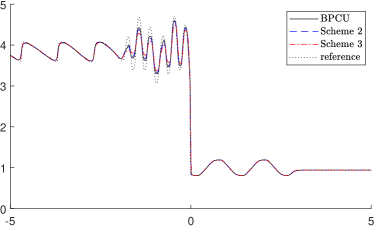
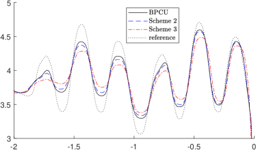
Figure 3. Example 4.2: Density ($\rho$) computed by the BPCU scheme and Schemes 2 and 3 (left) and zoom at the smooth part of $\rho$ (right).

Example 4.3.

We consider the “123 problem” from [8]: this is a Riemann problem, whose exact solution consists of two rarefaction waves and a near-vacuum region between them. The initial data,

$$(\rho(x,0),u(x,0),p(x,0))=\left\{\begin{aligned} &(1,-2,0.15)&&x<0.5,\\ &(1,2,0.15),&&x>0.5,\end{aligned}\right.$$

are prescribed on the computational domain $[0,1]$ subject to free boundary conditions.

We compute the solution by the proposed BPCU scheme until time $t=0.15$ on a uniform mesh with $\Delta x=1/200$. The obtained density and pressure are depicted in Figure 4, which clearly shows two rarefaction waves and the near vacuum region in the middle. We also plot the minimum of both density and pressure as functions of time in Figure 4: these graphs demonstrates that the positivity of density and pressure is preserved by the BPCU scheme. On the other hand, Scheme 1 violates the BP property at the second stage of first Runge-Kutta time step by producing a negative pressure value $p\approx-2.43\times 10^{-2}$.

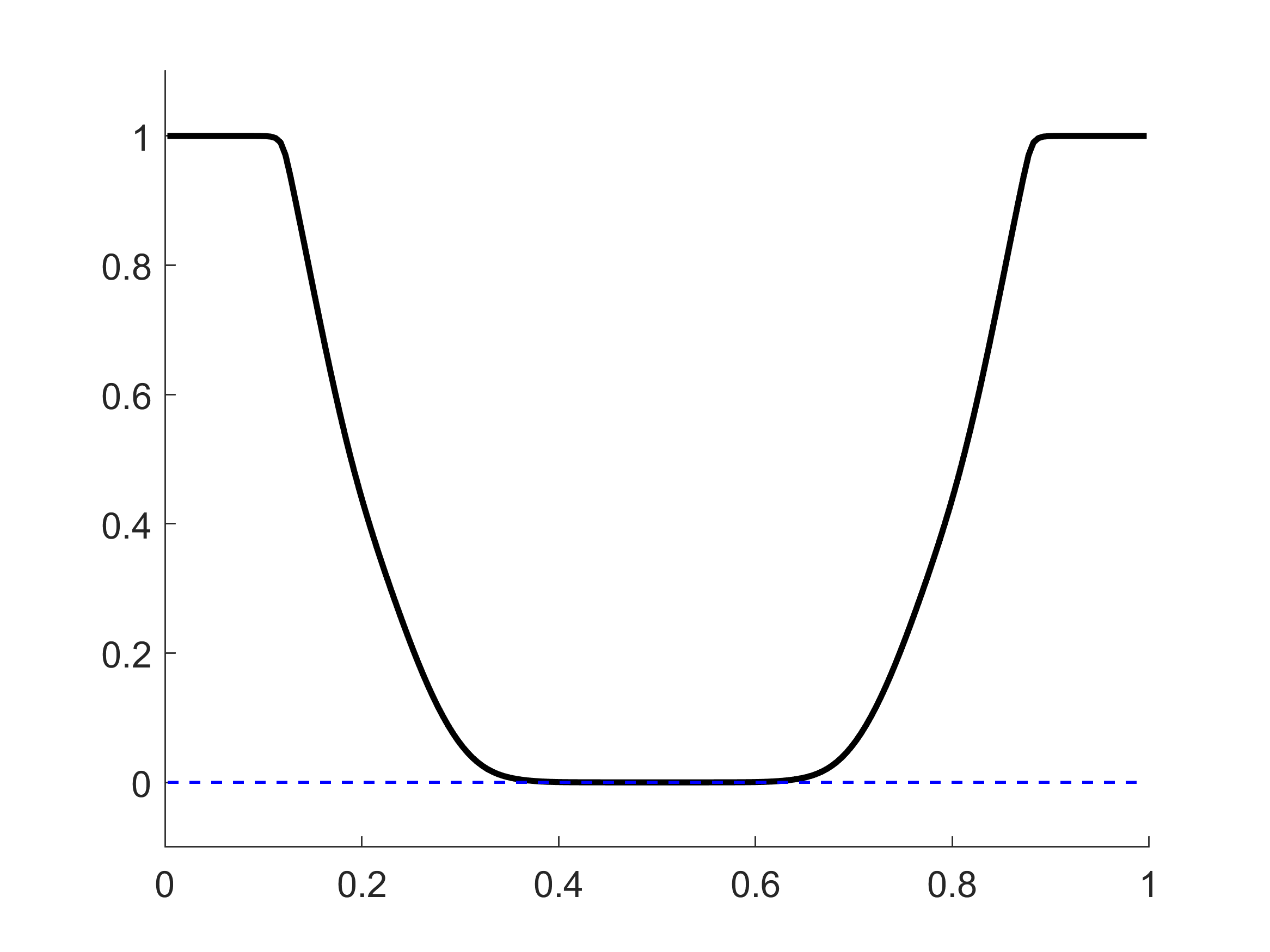
(a) density at $t=0.15$

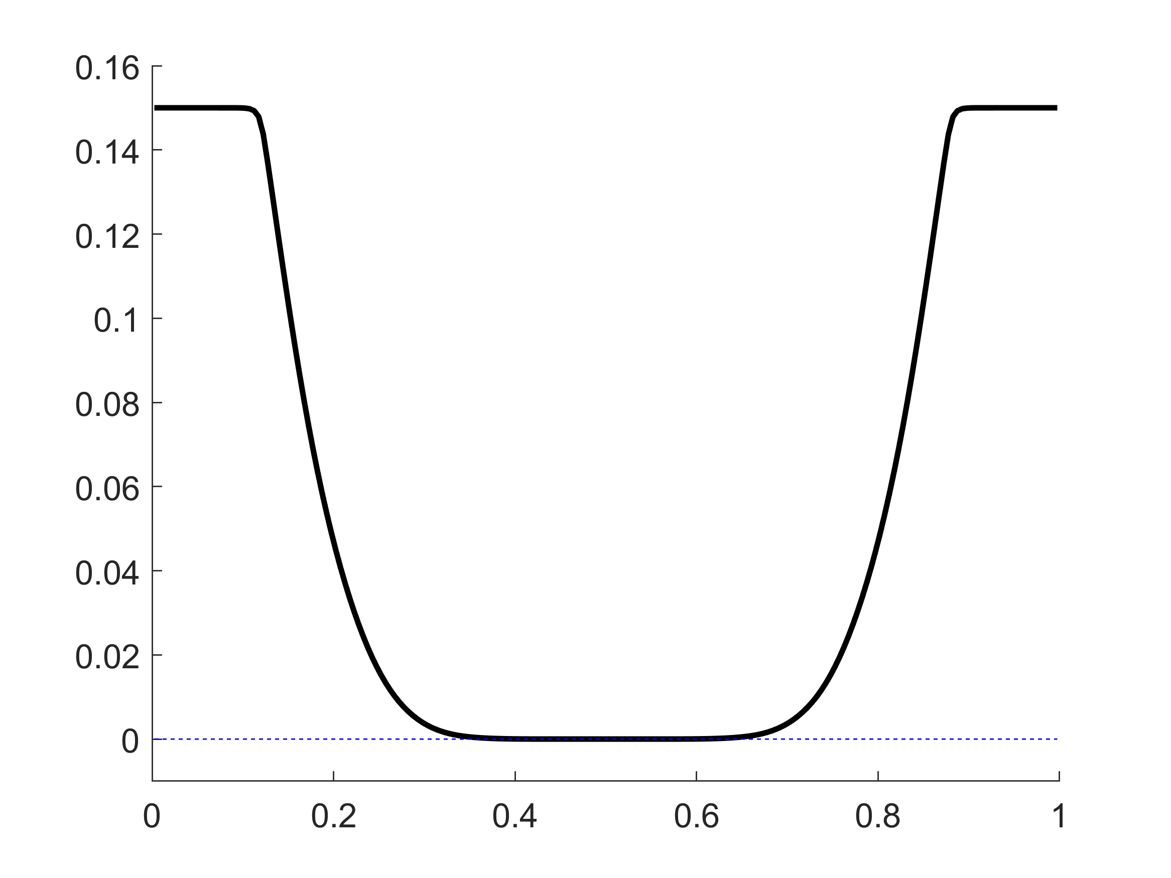
(b) pressure at $t=0.15$

(c) minimum density as a function of time

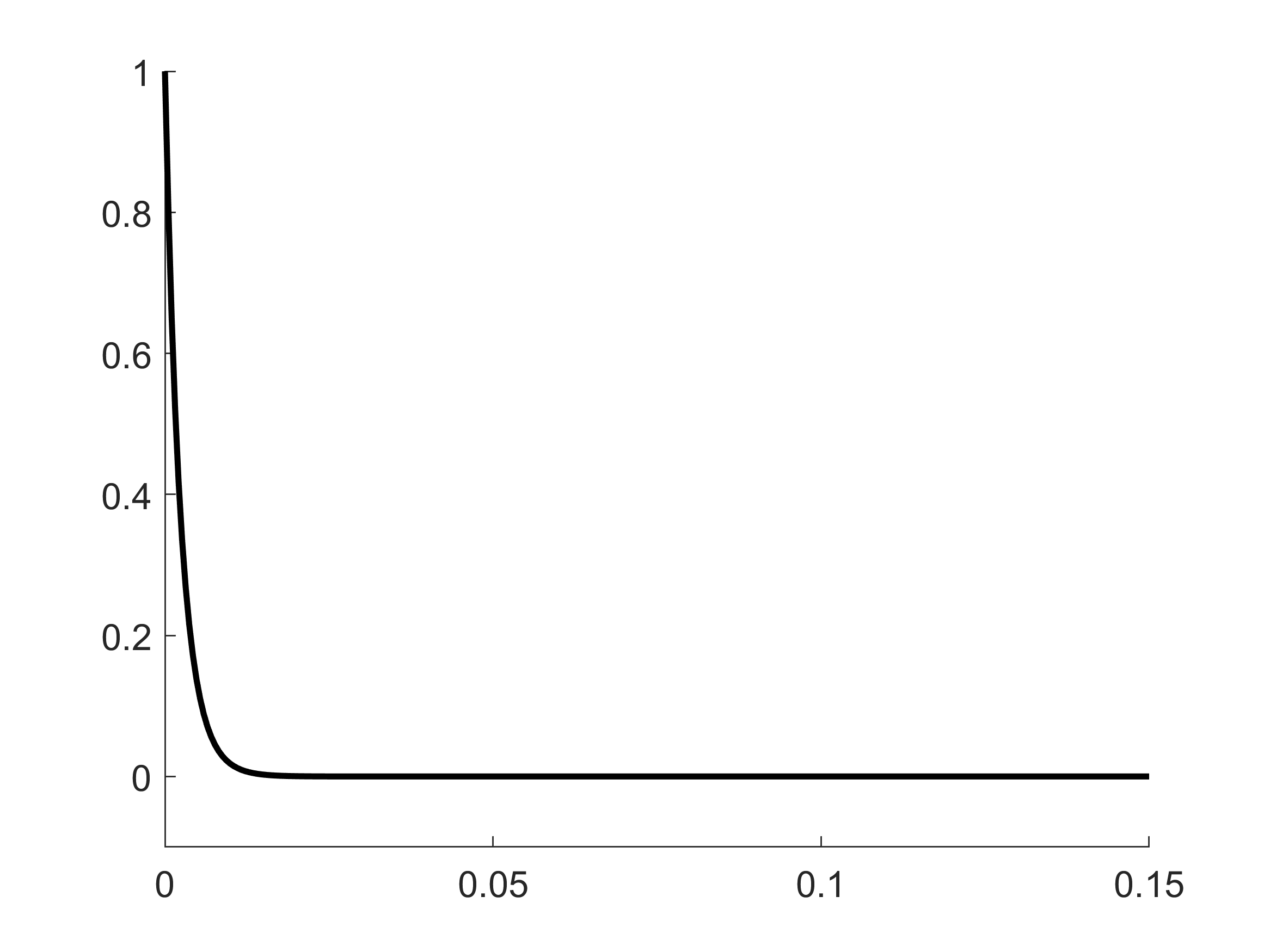
(d) minimum pressure as a function of time

Figure 4. Example 4.3: Density ($\rho$) and pressure ($p$) computed by the BPCU scheme.

Example 4.4.

In this example taken from [12, 50], we simulate a Mach 80 jet. Initially, the computational domain $[0,2]\times[-0.5,0.5]$ is filled with the ambient gas with $\rho(x,y,0)\equiv 5$, $v_{1}(x,y,0)=v_{2}(x,y,0)\equiv 0$, and $p(x,y,0)\equiv 0.4127$. From the left boundary between $y=-0.05$ and 0.05, a jet of state $(\rho,v_{1},v_{2},p)=(5,30,0,0.4127)$ is injected into the computational domain, and free boundary conditions are imposed on all other boundaries.

We compute the solution by the BPCU scheme until time $t=0.07$ on a uniform mesh containing $448\times 224$ cells. The snapshots of the numerical solution at times $t=0.05$ and 0.07, presented in Figure 5, agree well with those reported in [50]. The BP property of the numerical scheme is crucial in this example: if Scheme 1 is used in this example, negative pressure will appear in the numerical result at $t\approx 5.277\times 10^{-4}$.

  

  

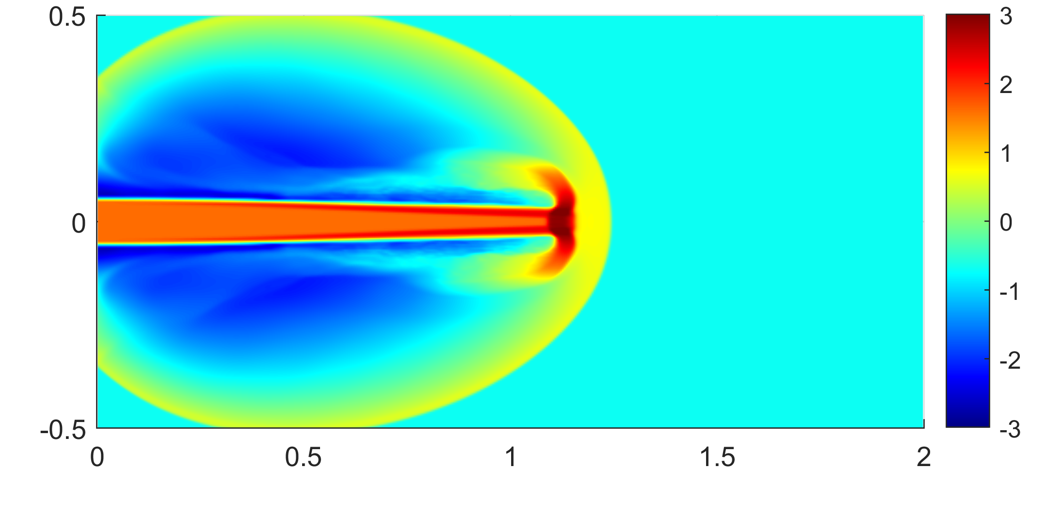
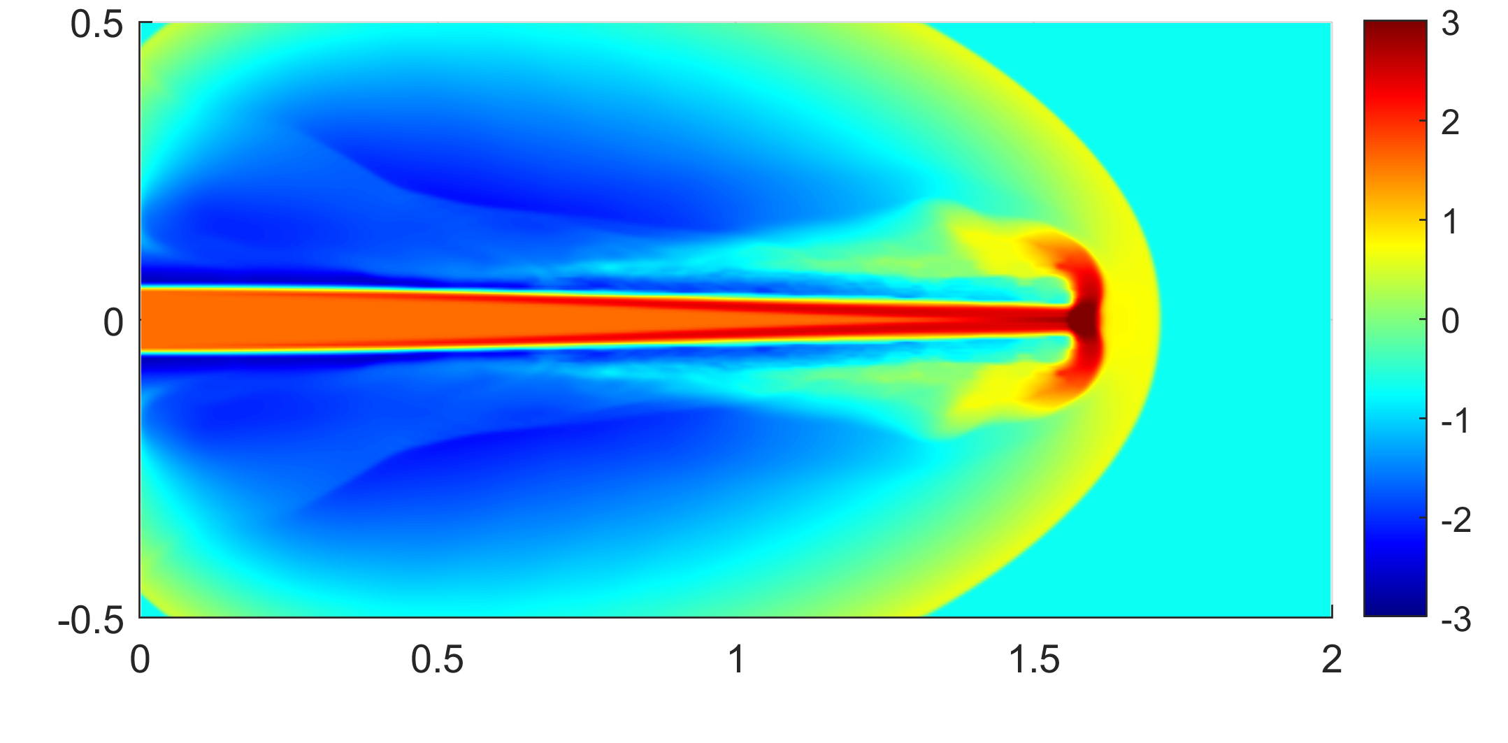
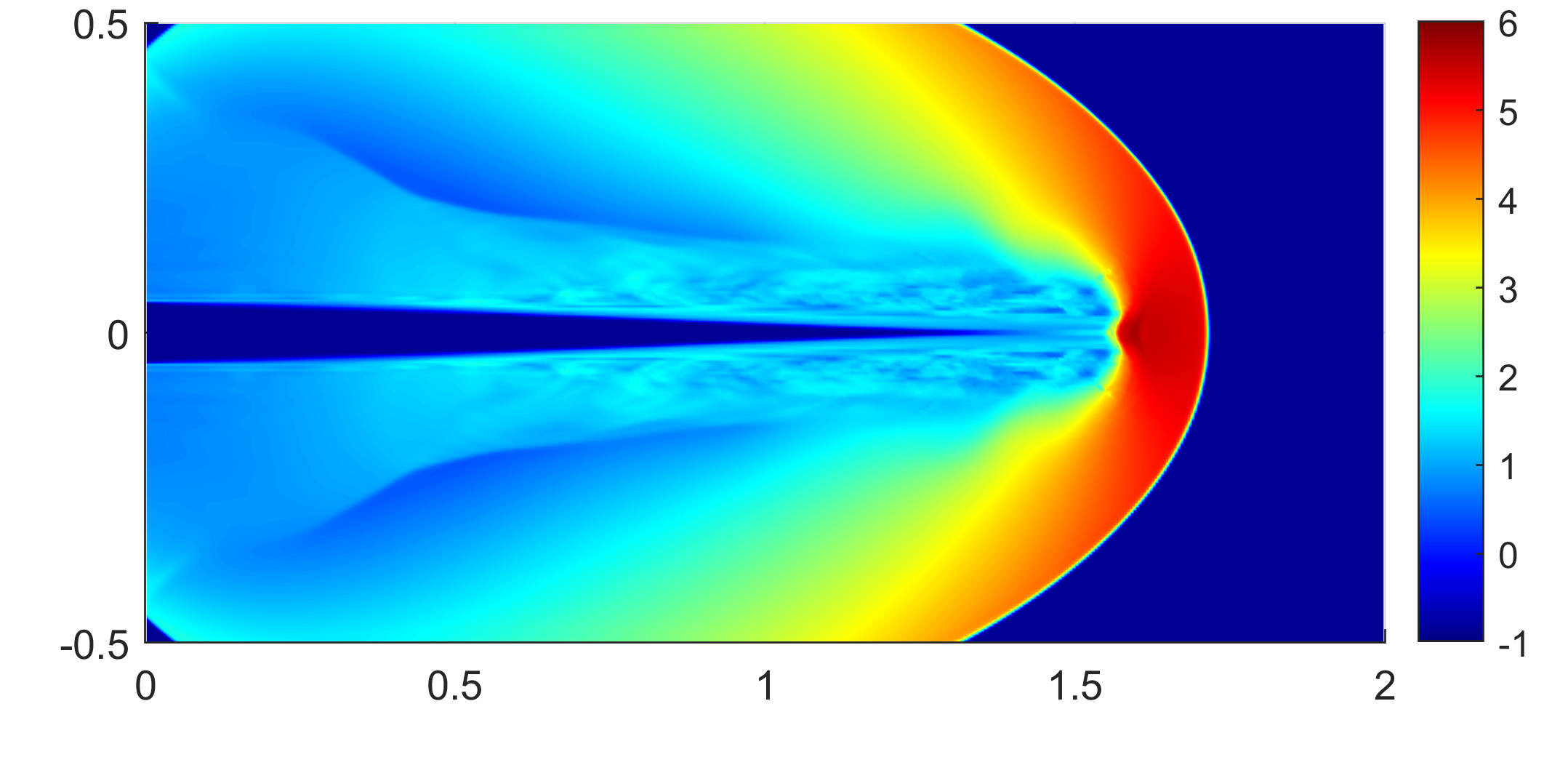
Figure 5. Example 4.4: Solution ($\ln\rho$ (top row) and $\ln p$ (bottom row)) computed by the BPCU scheme at times $t=0.05$ (left column) and 0.07 (right column).

Example 4.5.

In this example taken from [50], a Mach 2000 jet is considered. The computational domain is $[0,1]\times[-0.25,0.25]$ and the initial and boundary conditions are the same as in Example 4.4, except for the jet state which is now $(\rho,v_{1},v_{2},p)=(5,800,0,0.4127)$.

We compute the solution by the BPCU scheme until time $t=0.0015$ on a uniform mesh containing $640\times 320$ cells. The snapshots of the numerical solution at times $t=0.001$ and 0.0015, presented in Figure 6, agree well with those reported in [50]. As in Example 4.4, if the BP property is not enforced, that is, if Scheme 1 is used, negative pressure will appear in the numerical solution at $t\approx 7.15\times 10^{-4}$.

  

  

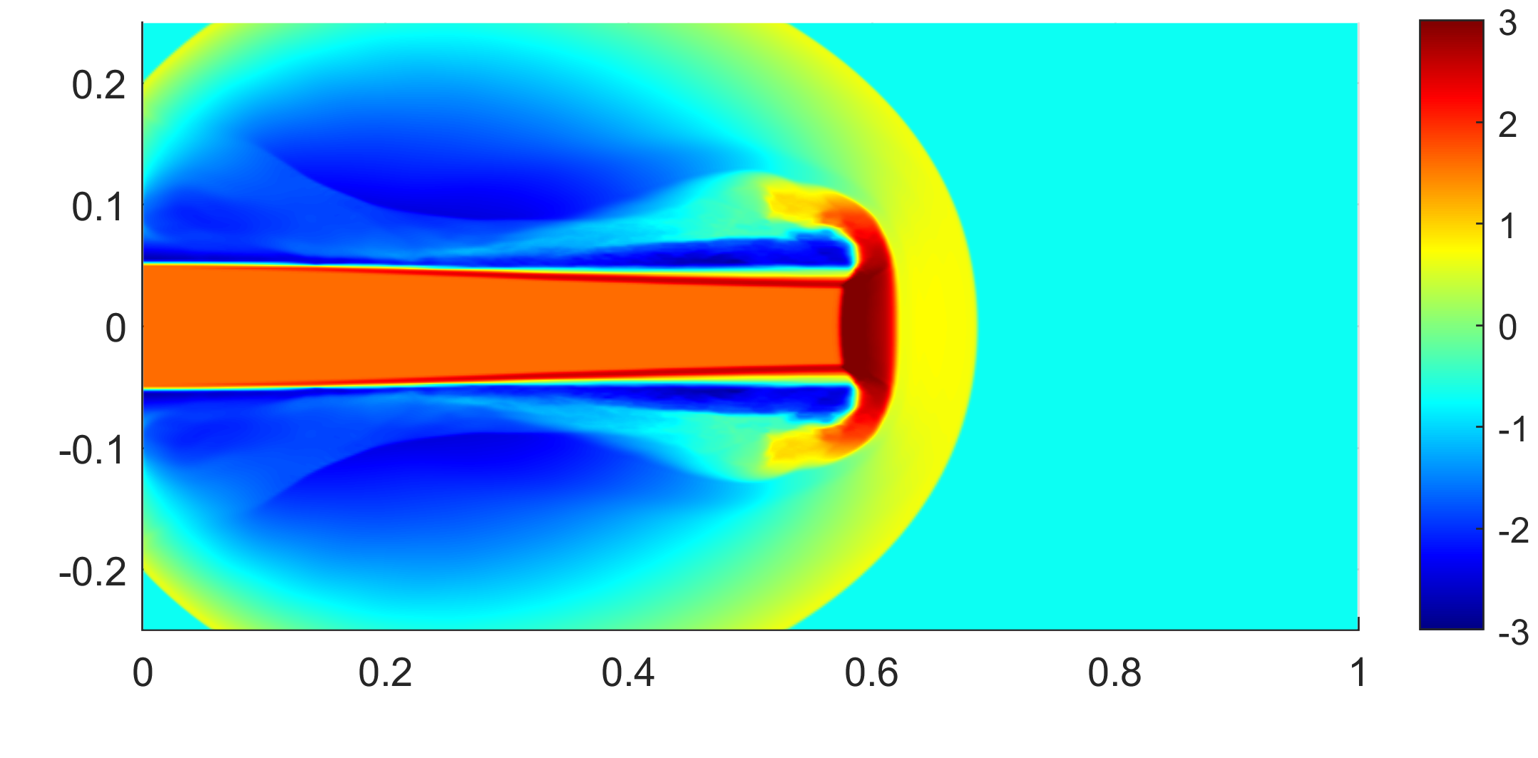
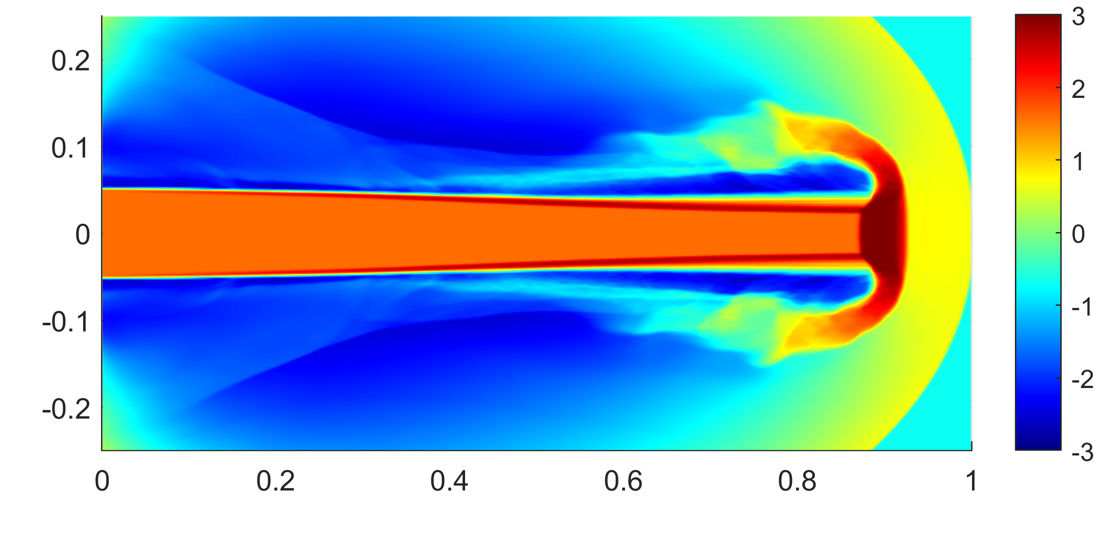
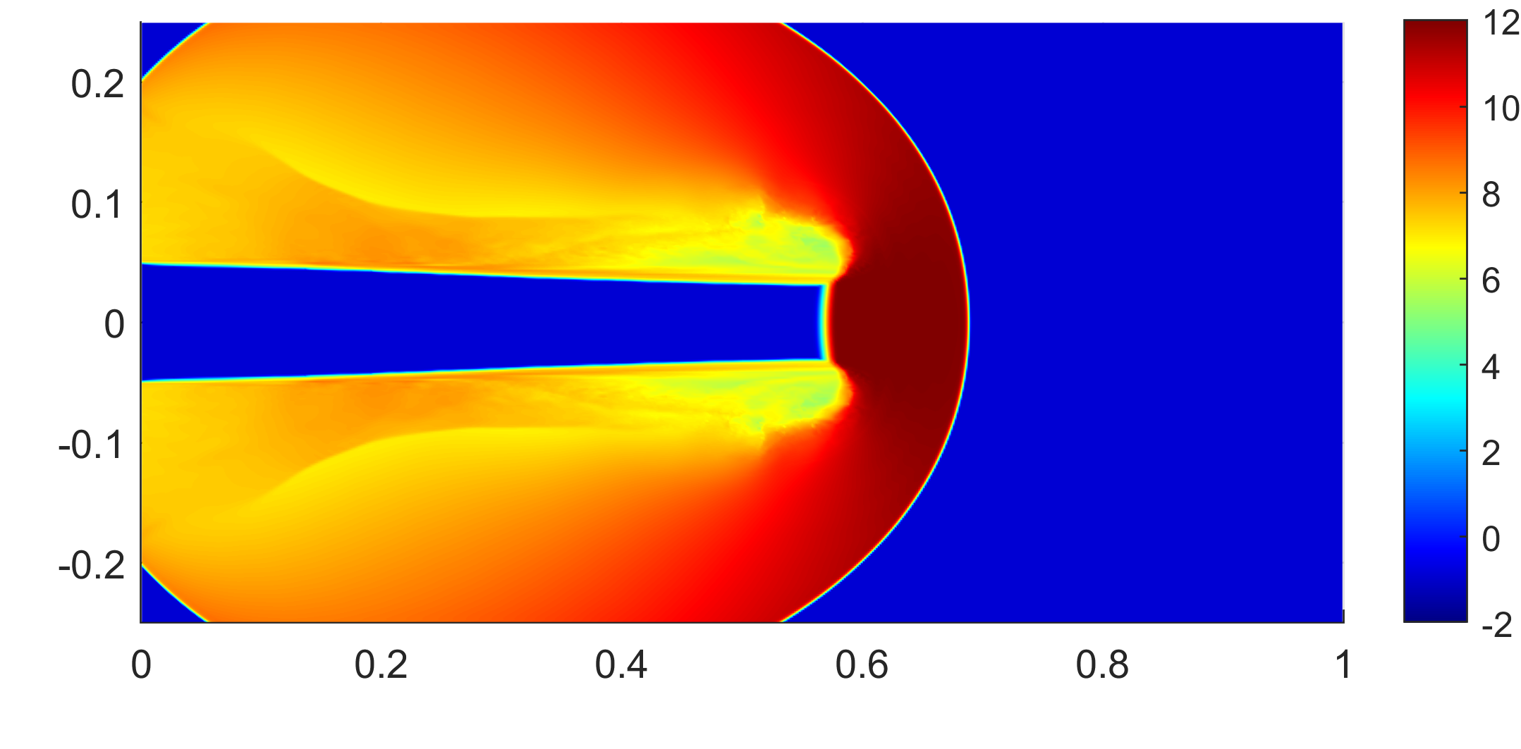
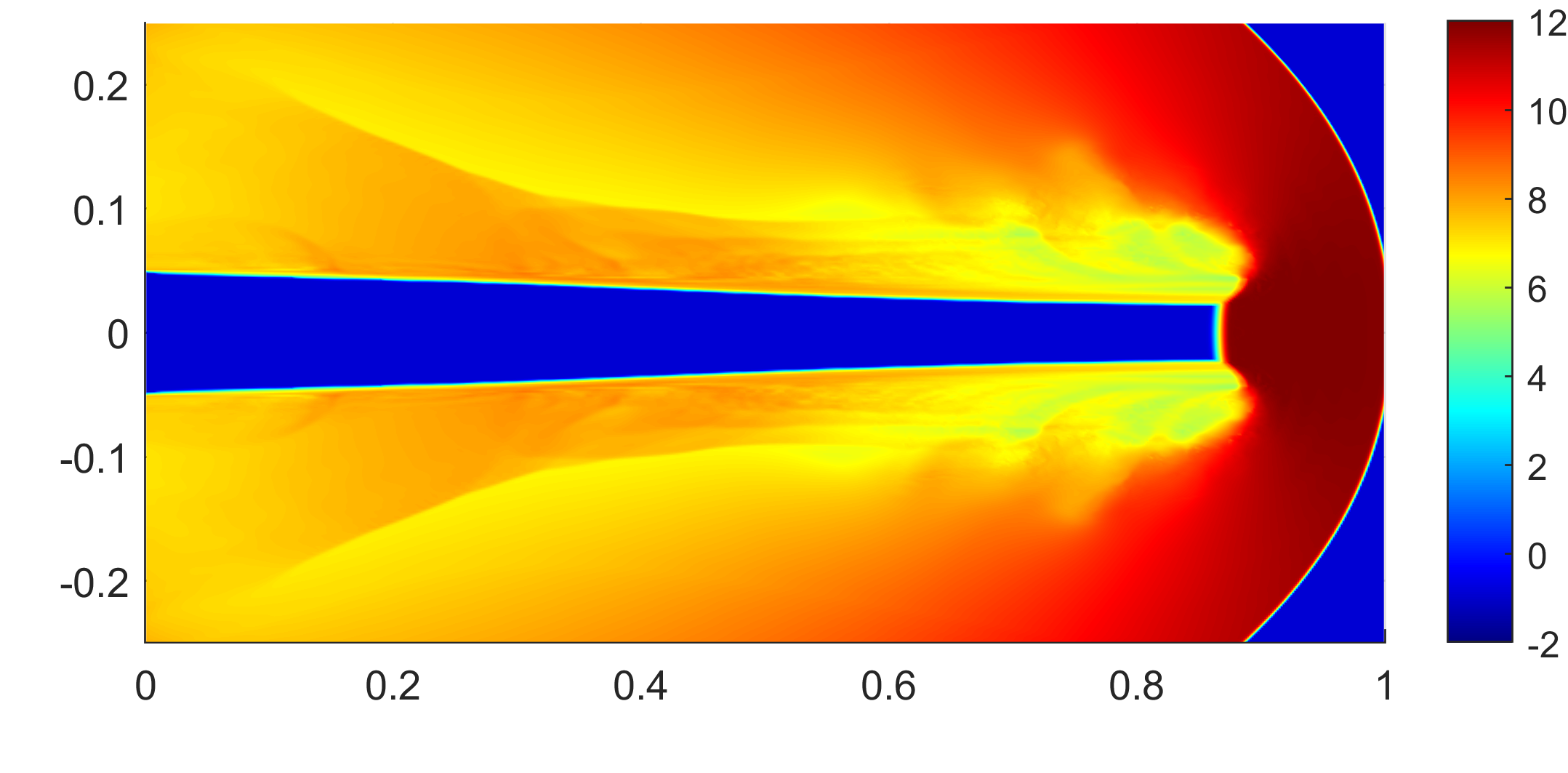
Figure 6. Example 4.5: Solution ($\ln\rho$ (top row) and $\ln p$ (bottom row)) computed by the BPCU scheme at times $t=0.001$ (left column) and 0.0015 (right column).

Example 4.6.

This is a shock diffraction benchmark taken from [26, 5, 50]. The computational domain is $[0,1]\times[6,11]\cup[1,13]\times[0,11]$. At time $t=0$, a pure right-moving shock of Mach number 5.09 is located at $x=0.5$ for $y\in[6,11]$. The inflow boundary conditions are imposed at $x=0$ for $y\in[6,11]$, free boundary conditions are used at $x=13$ for $y\in[1,11]$, at $y=0$ for $x\in[1,13]$, and at $y=11$ for $x\in[0,13]$, and solid wall boundary conditions are specified at $y=6$ for $x\in[0,1]$ and at $x=1$ for $y\in[0,6]$.

Density and pressure computed by the BPCU scheme at time $t=2.3$ on a uniform mesh with $\Delta x=\Delta y=1/64$, are presented in Figure 7. The results agree well to those reported in [26, 5, 50]. We emphasize that this example is challenging due to the very low density and pressure. Numerical schemes that do not satisfy the BP property may generate negative pressure and/or density values, leading to failures of computation. For instance, Scheme 1 produces negative pressure at $t\approx 0.1074$.

  

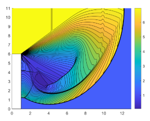
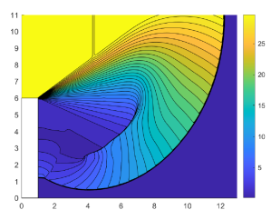
Figure 7. Example 4.6: Density ($\rho$): 40 equally spaced contour lines from 0.066227 to 7.1568 (left) and pressure ($p$): 40 equally spaced contour lines from 0.091 to 37.3 (right) computed by the BPCU scheme.

Example 4.7.

The last example is the benchmark from [30] of flow past a forward facing step. Initially, a right-going Mach 3 uniform flow enters a wind tunnel $[0,1]\times[0,3]$, initially filled with a gas with $\rho(x,y,0)\equiv 1.4$, $u(x,y,0)\equiv 3$, $v(x,y,0)\equiv 0$, and $p(x,y,0)\equiv 1$. The step of height 0.2 is located at $x=0.6$. Solid wall boundary conditions are applied along the walls of the tunnel. The inflow and free boundary conditions are applied at the entrance ($x=0$) and the exit ($x=3$), respectively.

We conduct the simulation on two uniform meshes: a coarser (with $\Delta x=\Delta y=1/160$) and a finer ($\Delta x=\Delta y=1/360$) ones. The density computed by the BPCU scheme as well as Scemes 2 and 3 at time $t=4$ are shown in Figure 8. As one can see, the BPCU scheme achieves higher resolution than its counterparts, especially for the slip line issued from the triple point near $(0.6,0.75)$.

(a) $\Delta x=\Delta y=1/160$, BPCU scheme

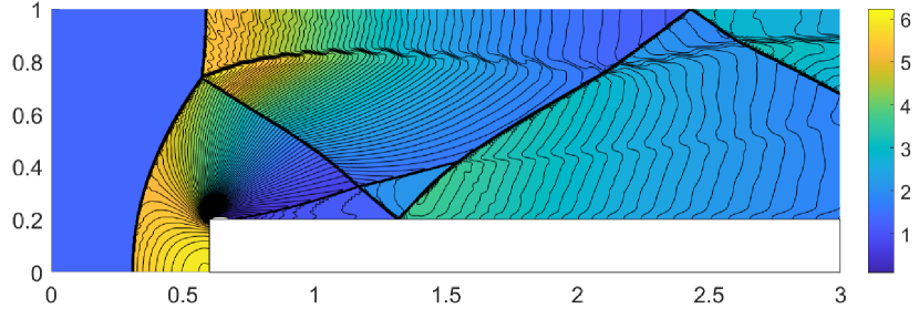
(b) $\Delta x=\Delta y=1/320$, BPCU scheme

(c) $\Delta x=\Delta y=1/160$, Scheme 2

(d) $\Delta x=\Delta y=1/320$, Scheme 2

(e) $\Delta x=\Delta y=1/160$, Scheme 3

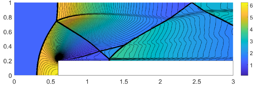
(f) $\Delta x=\Delta y=1/320$, Scheme 3

Figure 8. Example 4.7: Density ($\rho$) computed by the BPCU scheme (top row), Scheme 2 (middle row), and Scheme 3 (bottom row) on the coarse (left column) and fine (right column) meshes. 80 equally spaced contour lines from $0.090338$ to $6.2365$.

5. Conclusions

In this paper, we have established a novel framework to analyze and develop bound-preserving (BP) central-upwind (CU) schemes for general hyperbolic systems of conservation laws. As the foundation of this framework, we have discovered that the CU schemes can be decomposed as a convex combination of several intermediate solution states. Thanks to this key finding, the goal of designing BPCU schemes was simplified to the enforcement of four more accessible BP conditions, each of which can be achieved by minor modification to the CU schemes. Our framework is applicable to general hyperbolic systems of conservation laws and as a specific application, we have employed it to construct provably BPCU schemes for one- and two-dimensional Euler equations of gas dynamics. The robustness and effectivenss of the proposed BPCU schemes have been validated by several challenging numerical examples.

References

- [1] P. Arminjon, M.-C. Viallon, and A. Madrane, A finite volume extension of the Lax-Friedrichs and Nessyahu-Tadmor schemes for conservation laws on unstructured grids, Int. J. Comput. Fluid Dyn. 9 (1997), 1–22.
- [2] S. Bryson, A. Kurganov, D. Levy, and G. Petrova, Semi-discrete central-upwind schemes with reduced dissipation for Hamilton-Jacobi equations, IMA J. Numer. Anal. 25 (2005), 113–138.
- [3] A. Chertock, S. Chu, M. Herty, A. Kurganov, and M. Lukáčová-Medvid’ová, Local characteristic decomposition based central-upwind scheme, J. Comput. Phys. 473 (2023), Paper No. 111718, 24 pp.
- [4] A. Chertock, S. Cui, A. Kurganov, Ş. N. Özcan, and E. Tadmor, Well-balanced schemes for the Euler equations with gravitation: Conservative formulation using global fluxes, J. Comput. Phys. 358 (2018), 36–52.
- [5] B. Cockburn and C.-W. Shu, The Runge-Kutta discontinuous Galerkin method for conservation laws. V. Multidimensional systems, J. Comput. Phys. 141 (1998), no. 2, 199–224.
- [6] Jie Du, Cheng Wang, Chengeng Qian, and Yang Yang, High-order bound-preserving discontinuous Galerkin methods for stiff multispecies detonation, SIAM J. Sci. Comput. 41 (2019), no. 2, B250–B273.
- [7] Jie Du and Yang Yang, Third-order conservative sign-preserving and steady-state-preserving time integrations and applications in stiff multispecies and multireaction detonations, J. Comput. Phys. 395 (2019), 489–510.
- [8] B. Einfeldt, C.-D. Munz, P. L. Roe, and B. Sjögreen, On Godunov-type methods near low densities, J. Comput. Phys. 92 (1991), no. 2, 273–295.
- [9] S. Gottlieb, D. Ketcheson, and C.-W. Shu, Strong stability preserving Runge-Kutta and multistep time discretizations, World Scientific Publishing Co. Pte. Ltd., Hackensack, NJ, 2011.
- [10] S. Gottlieb, C.-W. Shu, and E. Tadmor, Strong stability-preserving high-order time discretization methods, SIAM Rev. 43 (2001), no. 1, 89–112.
- [11] Jean-Luc Guermond and Bojan Popov, Invariant domains and second-order continuous finite element approximation for scalar conservation equations, SIAM J. Numer. Anal. 55 (2017), no. 6, 3120–3146.
- [12] Youngsoo Ha, Carl L. Gardner, Anne Gelb, and C.-W. Shu, Numerical simulation of high Mach number astrophysical jets with radiative cooling, J. Sci. Comput. 24 (2005), no. 1, 29–44.
- [13] Xiangyu Y Hu, Nikolaus A Adams, and Chi-Wang Shu, Positivity-preserving method for high-order conservative schemes solving compressible Euler equations, J. Comput. Phys. 242 (2013), 169–180.
- [14] G.-S. Jiang and E. Tadmor, Nonoscillatory central schemes for multidimensional hyperbolic conservation laws, SIAM J. Sci. Comput. 19 (1998), no. 6, 1892–1917 (electronic).
- [15] Yi Jiang and Hailiang Liu, Invariant-region-preserving DG methods for multi-dimensional hyperbolic conservation law systems, with an application to compressible Euler equations, J. Comput. Phys. 373 (2018), 385–409.
- [16] A. Kurganov, S. Noelle, and G. Petrova, Semidiscrete central-upwind schemes for hyperbolic conservation laws and Hamilton-Jacobi equations, SIAM J. Sci. Comput. 23 (2001), no. 3, 707–740.
- [17] A. Kurganov and E. Tadmor, New high-resolution central schemes for nonlinear conservation laws and convection-diffusion equations, J. Comput. Phys. 160 (2000), no. 1, 241–282.
- [18] by same author, Solution of two-dimensional Riemann problems for gas dynamics without Riemann problem solvers, Numer. Methods Partial Differential Equations 18 (2002), no. 5, 584–608.
- [19] A. Kurganov and R. Xin, New low-dissipation central-upwind schemes, J. Sci. Comput. 96 (2023), Paper No. 56, 33 pp.
- [20] Alexander Kurganov and Chi-Tien Lin, On the reduction of numerical dissipation in central-upwind schemes, Commun. Comput. Phys. 2 (2007), no. 1, 141–163. MR 2305919
- [21] D. Levy, G. Puppo, and G. Russo, Central WENO schemes for hyperbolic systems of conservation laws, M2AN Math. Model. Numer. Anal. 33 (1999), no. 3, 547–571.
- [22] K.-A. Lie and S. Noelle, On the artificial compression method for second-order nonoscillatory central difference schemes for systems of conservation laws, SIAM J. Sci. Comput. 24 (2003), no. 4, 1157–1174.
- [23] X.-D. Liu and E. Tadmor, Third order nonoscillatory central scheme for hyperbolic conservation laws, Numer. Math. 79 (1998), no. 3, 397–425.
- [24] H. Nessyahu and E. Tadmor, Nonoscillatory central differencing for hyperbolic conservation laws, J. Comput. Phys. 87 (1990), no. 2, 408–463.
- [25] Tong Qin, Chi-Wang Shu, and Yang Yang, Bound-preserving discontinuous Galerkin methods for relativistic hydrodynamics, J. Comput. Phys. 315 (2016), 323–347.
- [26] J. J. Quirk, A contribution to the great Riemann solver debate, Internat. J. Numer. Methods Fluids 18 (1994), no. 6, 555–574.
- [27] C.-W. Shu and S. Osher, Efficient implementation of essentially nonoscillatory shock-capturing schemes. II, J. Comput. Phys. 83 (1989), no. 1, 32–78.
- [28] P. K. Sweby, High resolution schemes using flux limiters for hyperbolic conservation laws, SIAM J. Numer. Anal. 21 (1984), no. 5, 995–1011.
- [29] Cheng Wang, Xiangxiong Zhang, Chi-Wang Shu, and Jianguo Ning, Robust high order discontinuous Galerkin schemes for two-dimensional gaseous detonations, J. Comput. Phys. 231 (2012), no. 2, 653–665.
- [30] P. Woodward and P. Colella, The numerical solution of two-dimensional fluid flow with strong shocks, J. Comput. Phys. 54 (1988), 115–173.
- [31] K. Wu, Design of provably physical-constraint-preserving methods for general relativistic hydrodynamics, Phys. Rev. D 95 (2017), no. 10, Paper No. 103001, 19 pp.
- [32] K. Wu, Positivity-preserving analysis of numerical schemes for ideal magnetohydrodynamics, SIAM J. Numer. Anal. 56 (2018), no. 4, 2124–2147.
- [33] K. Wu and C.-W. Shu, A provably positive discontinuous Galerkin method for multidimensional ideal magnetohydrodynamics, SIAM J. Sci. Comput. 40 (2018), no. 5, B1302–B1329.
- [34] K. Wu and C.-W. Shu, Geometric quasilinearization framework for analysis and design of bound-preserving schemes, SIAM Rev. 65 (2023), no. 4, 1031–1073.
- [35] Kailiang Wu, Minimum principle on specific entropy and high-order accurate invariant region preserving numerical methods for relativistic hydrodynamics, SIAM J. Sci. Comput. 43 (2021), no. 6, B1164–B1197.
- [36] Kailiang Wu, Haili Jiang, and Chi-Wang Shu, Provably positive central discontinuous Galerkin schemes via geometric quasilinearization for ideal MHD equations, SIAM J. Numer. Anal. 61 (2023), no. 1, 250–285.
- [37] Kailiang Wu and Chi-Wang Shu, Provably positive high-order schemes for ideal magnetohydrodynamics: analysis on general meshes, Numer. Math. 142 (2019), no. 4, 995–1047.
- [38] by same author, Provably physical-constraint-preserving discontinuous Galerkin methods for multidimensional relativistic MHD equations, Numer. Math. 148 (2021), 699–741.
- [39] Kailiang Wu and Huazhong Tang, High-order accurate physical-constraints-preserving finite difference WENO schemes for special relativistic hydrodynamics, J. Comput. Phys. 298 (2015), 539–564.
- [40] by same author, Admissible states and physical-constraints-preserving schemes for relativistic magnetohydrodynamic equations, Math. Models Methods Appl. Sci. 27 (2017), no. 10, 1871–1928.
- [41] Yulong Xing, Xiangxiong Zhang, and Chi-Wang Shu, Positivity-preserving high order well-balanced discontinuous Galerkin methods for the shallow water equations, Adv. Water Resour. 33 (2010), no. 12, 1476–1493.
- [42] Tao Xiong, Jing-Mei Qiu, and Zhengfu Xu, Parametrized positivity preserving flux limiters for the high order finite difference WENO scheme solving compressible Euler equations, J. Sci. Comput. 67 (2016), no. 3, 1066–1088.
- [43] Z. Xu and X. Zhang, Bound-preserving high-order schemes, Handbook of numerical methods for hyperbolic problems, Handb. Numer. Anal., vol. 18, Elsevier/North-Holland, Amsterdam, 2017, pp. 81–102.
- [44] Zhengfu Xu, Parametrized maximum principle preserving flux limiters for high order schemes solving hyperbolic conservation laws: one-dimensional scalar problem, Math. Comp. 83 (2014), no. 289, 2213–2238.
- [45] R. Yan, W. Tong, and G. Chen, An efficient invariant-region-preserving central scheme for hyperbolic conservation laws, Appl. Math. Comput. 436 (2023), Paper No. 127500, 18 pp.
- [46] X. Zhang and C.-W. Shu, Maximum-principle-satisfying and positivity-preserving high-order schemes for conservation laws: survey and new developments, Proc. R. Soc. A 467 (2011), 2752–2776.
- [47] X. Zhang, Y. Xia, and C.-W. Shu, Maximum-principle-satisfying and positivity-preserving high order discontinuous Galerkin schemes for conservation laws on triangular meshes, J. Sci. Comput. 50 (2012), no. 1, 29–62.
- [48] Xiangxiong Zhang, On positivity-preserving high order discontinuous Galerkin schemes for compressible Navier-Stokes equations, J. Comput. Phys. 328 (2017), 301–343.
- [49] Xiangxiong Zhang and Chi-Wang Shu, On maximum-principle-satisfying high order schemes for scalar conservation laws, J. Comput. Phys. 229 (2010), no. 9, 3091–3120.
- [50] by same author, On positivity-preserving high order discontinuous Galerkin schemes for compressible Euler equations on rectangular meshes, J. Comput. Phys. 229 (2010), no. 23, 8918–8934.
- [51] Y. Zhang, X. Zhang, and C.-W. Shu, Maximum-principle-satisfying second order discontinuous Galerkin schemes for convection-diffusion equations on triangular meshes, J. Comput. Phys. 234 (2013), 295–316.