Fourth-order entropy-stable lattice Boltzmann schemes for hyperbolic systems

Abstract

We present a novel framework for the development of fourth-order lattice Boltzmann schemes to tackle multidimensional nonlinear systems of conservation laws. Our numerical schemes preserve two fundamental characteristics inherent in classical lattice Boltzmann methods: a local relaxation phase and a transport phase composed of elementary shifts on a Cartesian grid. Achieving fourth-order accuracy is accomplished through the composition of second-order time-symmetric basic schemes utilizing rational weights. This enables the representation of the transport phase in terms of elementary shifts. Introducing local variations in the relaxation parameter during each stage of relaxation ensures the entropic nature of the schemes. This not only enhances stability in the long-time limit but also maintains fourth-order accuracy. To validate our approach, we conduct comprehensive testing on scalar equations and systems in both one and two spatial dimensions.

Keywords— lattice Boltzmann, fourth-order, hyperbolic systems of conservation laws, entropy

MSC— 76M28, 65M99, 65M12

Introduction

Lattice Boltzmann schemes [25] have gained acclaim for their computational efficiency and ease of use on modern computer architectures (e.g. GPUs), owing to their distinctive structure, comprising a local collision/relaxation phase and a linear transport phase. The latter is constructed through shifts of data on a regular Cartesian grid. Despite their recent application in simulating non-linear systems of conservation laws [19, 23, 17, 9, 8, 4, 24], these methods exhibit lower accuracy for such problems compared to more conventional approaches like Finite Volumes and Discontinuous Galerkin methods.

While the attainment of second-order accuracy in lattice Boltzmann schemes is well-understood, achieved by setting relaxation parameters to two [16, 20, 6], obtaining third and fourth-order accuracy proves to be a more intricate challenge [20]. The ability to increase the order is not guaranteed a priori—especially for non-linear equations—and depends on the specific lattice Boltzmann scheme in use. When possible, higher accuracy is attained by delicately tuning equilibria that do not contribute to consistency at the leading order, a process that can be complex. Moreover, it is challenging to ascertain the stability of the scheme under such modifications. Consequently, the only fourth-order schemes identified so far only address linear scalar equations in 1D [14, 5], with minimal practical significance.

This contribution aims at establishing a comprehensive framework for constructing fourth-order kinetic schemes for non-linear systems of multi-dimensional conservation laws. To achieve this objective, a departure from standard lattice Boltzmann schemes is necessary. Nevertheless, the numerical schemes to be developed maintain the two keys to success of any standard lattice Boltzmann scheme, namely the locality of the collision phase and a transport phase made up of simple shifts, thus retain their notorious efficiency, compared to standard kinetic schemes [29, 1]. The essential idea to increase the order of the schemes is to allow both forward and backward steps in time.

In the whole paper, we are going to deal mostly with smooth solutions : the development of limiting procedures in the context of lattice Boltzmann schemes remains an open and fundamental question worth thorough discussions that we will not address in the present contribution. The present contribution aims at being a proof of concept of a new paradigm to construct high-order lattice Boltzmann schemes for general hyperbolic problems.

The paper is organized as follows. In Section 1, we introduce the system of conservation laws addressed in this paper, along with its relaxation approximation, facilitating the handling of non-linearity. Section 2 outlines our numerical strategy, beginning with a conventional lattice Boltzmann scheme, followed by a time-symmetrization step [15], and eventual composition to achieve fourth-order accuracy [32]. We finish on brief considerations about stability, specifically in terms of the $L^{2}$ norm in a basic scalar linear setting. A first batch of numerical experiments, presented in Section 3, empirically confirms the theoretical predictions. In Section 4, we introduce a method for adjusting the relaxation parameter to ensure entropy stability for the numerical scheme. The need for this procedure and the fact that it does not alter the order of the scheme are studied by means of new numerical experiments in Section 5. Finally, in Section 6, we propose, study, and test several variations on our fourth-order scheme. We eventually conclude in Section 7.

1 Target system of conservation laws and relaxation approximation

1.1 Target system of conservation laws

We aim at approximating the solution of the system on $\bm{u}:\mathbb{R}\times\mathbb{R}^{d}\to\mathbb{R}^{M}$:

$$\partial_{t}\bm{u}+\sum_{j=1}^{d}\frac{\partial}{\partial x_{j}}\bm{\varphi}^{j}(\bm{u})=0,$$ (1)

where $\bm{\varphi}^{j}:\mathbb{R}^{M}\to\mathbb{R}^{M}$ for $j\in\llbracket 1,d\rrbracket$ are smooth and possibly non-linear fluxes, see [22]. To give a simple example, taking $d=1$, $M=1$, and $\varphi(u)=\tfrac{1}{2}u^{2}$ yields the inviscid Burgers equation. We assume that (1) admits a Lax entropy–entropy fluxes pair $(S,{{G}}^{1},\dots,{{G}}^{d})$, with $S:\mathbb{R}^{M}\to\mathbb{R}$ and ${{G}}^{j}:\mathbb{R}^{M}\to\mathbb{R}$ for $j\in\llbracket 1,d\rrbracket$, such that ${\nabla_{\bm{u}}\bm{\varphi}}^{j}\nabla_{\bm{u}}S=\nabla_{\bm{u}}{G}^{j}$ with $S$ convex. Further properties on this construction can be found in [10, 11].

1.2 Relaxation systems

In order to isolate the non-linearity of the fluxes appearing in (1) into a local relaxation term which is easily tractable, we consider the following discrete-velocity BGK relaxation systems [10, 2, 11] on the distribution functions $\bm{f}_{1},\dots,\bm{f}_{q}:\mathbb{R}\times\mathbb{R}^{d}\to\mathbb{R}^{M}$, under the form

$$\partial_{t}\bm{f}_{k}+\sum_{j=1}^{d}V_{k}^{j}\frac{\partial\bm{f}_{k}}{\partial x_{j}}=-\frac{1}{\epsilon}(\bm{f}_{k}-\bm{f}^{\textnormal{eq}}_{k}(\bm{u})),\qquad k\in\llbracket 1,q\rrbracket.$$ (2)

Here, $q\geq 2$ is the number of discrete velocities, which are $\bm{V}_{k}\in\mathbb{R}^{d}$, $\bm{u}=\sum_{k=1}^{k=q}\bm{f}_{k}$, and we indicate the relaxation time by $\epsilon>0$. Moreover, the equilibria $\bm{f}^{\textnormal{eq}}_{k}$ are non-linear functions of $\bm{u}$ and fulfill the compatibility relations

$$\bm{u}=\sum_{k=1}^{q}\bm{f}^{\textnormal{eq}}_{k}(\bm{u}),\qquad\bm{\varphi}^{j}(\bm{u})=\sum_{k=1}^{q}{V}_{k}^{j}\bm{f}^{\textnormal{eq}}_{k}(\bm{u}),\quad j\in\llbracket 1,d\rrbracket,$$ (3)

under which, the formal limit $\epsilon\to 0^{+}$ gives that $\bm{f}_{k}\approx\bm{f}^{\textnormal{eq}}_{k}$ and that the sum of the distribution functions under (2) approximates (1), see [2, 29].

For future use, we introduce the microscopic entropy [18] given by the sum of the kinetic entropies: $\Sigma(\bm{f}_{1},\dots,\bm{f}_{k})=\sum_{k=1}^{k=q}s_{k}(\bm{f}_{k})$, where the kinetic entropies $s_{1},\dots,s_{q}:\mathbb{R}^{M}\to\mathbb{R}$ are convex functions of their argument under the so-called characteristic condition, which will be visible in a moment. We also have

$$S(\bm{u})=\min_{\bm{u}=\sum_{k=1}^{k=q}\bm{f}_{k}}\Sigma(\bm{f}_{1},\dots,\bm{f}_{k})=\Sigma(\bm{f}_{1}^{\textnormal{eq}}(\bm{u}),\dots,\bm{f}_{k}^{\textnormal{eq}}(\bm{u})).$$ (4)

This expression means that the entropy $S$ stems from a constrained optimization of the microscopic entropy $\Sigma$, and that the minimum is reached on the equilibrium. Furthermore, equation (4) tells us that the entropy is an inf-convolution of the kinetic entropies [24], that translates—thanks to the Legendre-Fenchel transform [34] that we shall indicate by a ^∗—into $S^{*}=\sum_{k=1}^{k=q}s^{*}_{k}$. We also additionally request that [18]

$${{{G}}}^{j,\star}:=\bm{\varphi}^{j}(\bm{u}(\bm{p}))\cdot\bm{p}-{{G}}^{j}(\bm{u}(\bm{p}))=\sum_{k=1}^{q}{V}_{k}^{j}s^{*}_{k},\quad j\in\llbracket 1,d\rrbracket,$$ (5)

where $\bm{p}=\nabla_{\bm{u}}S$ is the conjugate variable. We here warn the readers about the difference between Legendre-Fenchel–transformed quantities, denoted by the symbol ^∗, and the notation employing a ^⋆ in (5).

Let us introduce the choices of discrete velocities and relaxation systems that we will address in the paper.

1.2.1 $d=1$: One-dimensional problems

We consider a two-velocities model, so we set $q=2$, having $V_{1}=V>0$ (which will be indexed by $+$, for the associated distribution function is transported in the positive direction) and $V_{2}=-V>0$ (which will be indexed by $-$). The only way of fulfilling (3) is to select the following equilibria:

$$\bm{f}_{\pm}^{\textnormal{eq}}(\bm{u})=\frac{1}{2}\bm{u}\pm\frac{1}{2V}\bm{\varphi}(\bm{u}).$$

Using the change of basis $\bm{u}=\bm{f}_{+}+\bm{f}_{-}$ and $\bm{v}=V(\bm{f}_{+}-\bm{f}_{-})$, (2) can be recast as

$$\begin{cases}\partial_{t}\bm{u}+\partial_{x}\bm{v}=0,\\ \partial_{t}\bm{v}+V^{2}\partial_{x}\bm{u}=-\frac{1}{\epsilon}(\bm{v}-\bm{\varphi}(\bm{u})),\end{cases}$$ (6)

being the well-known Jin-Xin relaxation system [27]. In the lattice Boltzmann nomenclature, this is a $\text{D}_{1}\text{Q}_{2}^{M}$ relaxation system [23].

Let us provide a few examples of problems that can be tackled using this scheme.

Example 1 (Linear transport equation).

Let $M=1$ and $\varphi(u)=au$. We consider the classic quadratic entropy given by $S(u)=\frac{1}{2}u^{2}$, thus the entropy flux is given by ${G}(u)=\frac{a}{2}u^{2}$. We obtain $S^{*}(p)=\frac{1}{2}p^{2}$ and ${G}^{\star}(p)=\frac{a}{2}p^{2}$ (observe that ${G}^{*}(p)=\frac{1}{2a}p^{2}$). The dual kinetic entropies satisfying the imposed constraints are

$$s^{*}_{\pm}(p)=\frac{1}{4}\Bigl{(}1\pm\frac{a}{V}\Bigr{)}p^{2},\qquad\text{thus}\qquad s_{\pm}(f_{\pm})=\frac{V}{V\pm a}(f_{\pm})^{2}.$$

The condition providing the convexity of the kinetic entropy is the celebrated sub-characteristic condition $|a|<V$.

Example 2 (Burgers equation).

Let $M=1$ and $\varphi(u)=\tfrac{1}{2}u^{2}$. We take $S(u)=\frac{1}{2}u^{2}$, thus the entropy flux is given by ${G}(u)=\frac{1}{3}u^{3}$. Analogously to the linear case, we obtain

$$s^{*}_{\pm}(p)=\frac{1}{4}p^{2}\pm\frac{1}{12V}p^{3},\qquad s_{\pm}(f_{\pm})=\frac{V^{2}}{6}\Bigl{(}\Bigl{(}1\pm\frac{4f_{\pm}}{V}\Bigr{)}^{3/2}\mp\frac{6f_{\pm}}{V}-1\Bigr{)}.$$

Again, convexity comes by $|u|<V$.

Example 3 (Shallow water system).

Let $M=2$, $\bm{u}={(u_{1},u_{2})}={(h,hu)}$, and $\bm{\varphi}(h,hu)={(hu,hu^{2}+\tfrac{g}{2}h^{2})}$ where $g>0$ is the gravity acceleration. As in [12, Section 3.2], we take $S(h,hu)=\tfrac{1}{2}hu^{2}+\tfrac{g}{2}h^{2}$, hence ${G}(h,hu)=\tfrac{1}{2}hu^{3}+\tfrac{g}{2}h^{2}u$. We have the dual variables $p_{1}=-\tfrac{1}{2}u^{2}+gh$ and $p_{2}=u$ and the dual kinetic entropies given by

$$s^{*}_{\pm}(\bm{p})=\frac{(V\pm p_{2})(2p_{1}+p_{2}^{2})^{2}}{16gV}.$$

Convexity comes under the condition $V>|u|+\sqrt{gh}$, see [24], which guarantees that the kinetic velocity is larger than the one of the fastest wave in the system. The kinetic entropies can be found analytically, albeit with complicated formulæ: they are given by $s_{\pm}(\bm{f}_{\pm})=\bm{p}_{\pm}(\bm{f}_{\pm})\cdot\bm{f}_{\pm}-s^{*}_{\pm}(\bm{p}_{\pm}(\bm{f}_{\pm}))$, where $\bm{p}_{\pm}(\bm{f}_{\pm})$ is the solution of $\bm{f}_{\pm}=\nabla_{\bm{p}}s^{*}_{\pm}(\bm{p}_{\pm})$. One can see that the first equation to solve is linear in $p_{\pm}^{1}$, thus we obtain

$$p_{\pm}^{1}(p_{\pm}^{2})=\frac{4Vgf_{\pm}^{1}-V(p_{\pm}^{2})^{2}\mp(p_{\pm}^{2})^{3}}{2(V\pm p_{\pm}^{2})},$$

which corresponds to a third-order equation on $p_{\pm}^{2}$ only:

$$\pm Vg(f_{\pm}^{1})^{2}+f_{\pm}^{1}(p_{\pm}^{2})^{3}-V^{2}f_{\pm}^{2}\pm(2Vf_{\pm}^{1}\mp f_{\pm}^{2})(p_{\pm}^{2})^{2}+(V^{2}f_{\pm}^{1}\pm 2Vf_{\pm}^{2})p_{\pm}^{2}=0.$$

This equation can be solved with the well-known formula for cubic equations, upon choosing a specific branch.

1.2.2 $d=2$: Two-dimensional problems

We consider a four-velocities model, so we set $q=4$, having $\bm{V}_{1}={(V,0)}$ (which will be indexed by $+,x$) with $V>0$, $\bm{V}_{2}={(0,V)}$ (indexed by $+,y$), $\bm{V}_{3}={(-V,0)}$ (indexed by $-,x$), and $\bm{V}_{4}={(0,-V)}$ (indexed by $-,y$). There are several ways of enforcing (3): the one we select is [21, Chapter 3]

$$\bm{f}^{\textnormal{eq}}_{\pm,x/y}(\bm{u})=\frac{1}{4}\bm{u}\pm\frac{1}{2V}\bm{\varphi}_{x/y}(\bm{u}).$$

Using the change of basis $\bm{u}=\bm{f}_{+,x}+\bm{f}_{+,y}+\bm{f}_{-,x}+\bm{f}_{-,y}$, $\bm{v}_{x}=V(\bm{f}_{+,x}-\bm{f}_{-,x})$, $\bm{v}_{y}=V(\bm{f}_{+,y}-\bm{f}_{-,y})$, and $\bm{w}=V^{2}(\bm{f}_{+,x}-\bm{f}_{+,y}-\bm{f}_{-,x}+\bm{f}_{-,y})$, we get

$$\begin{cases}\partial_{t}\bm{u}+\partial_{x}\bm{v}_{x}+\partial_{y}\bm{v}_{y}=0,\\ \partial_{t}\bm{v}_{x}+V^{2}\partial_{x}\bigl{(}\tfrac{1}{2}\bm{u}+\tfrac{1}{2V^{2}}\bm{w}\bigr{)}=-\frac{1}{\epsilon}(\bm{v}_{x}-\bm{\varphi}_{x}(\bm{u})),\\ \partial_{t}\bm{v}_{y}+V^{2}\partial_{y}\bigl{(}\tfrac{1}{2}\bm{u}-\tfrac{1}{2V^{2}}\bm{w}\bigr{)}=-\frac{1}{\epsilon}(\bm{v}_{y}-\bm{\varphi}_{y}(\bm{u})),\\ \partial_{t}\bm{w}+V^{2}\partial_{x}\bm{v}_{x}-V^{2}\partial_{y}\bm{v}_{y}=-\frac{1}{\epsilon}\bm{w}.\end{cases}$$ (7)

This can be called a $\text{D}_{2}\text{Q}_{4}^{M}$ relaxation system [19].

Example 4 (Linear transport equation).

Let $M=1$ and ${\varphi}^{1}(u)=(a_{x}u)$, ${\varphi}^{2}(u)=a_{y}u$. We consider $S(u)=\frac{1}{2}u^{2}$, thus the entropy flux is given by ${{G}}(u)=(\frac{a_{x}}{2}u^{2},\frac{a_{y}}{2}u^{2})$. We obtain $S^{*}(p)=\frac{1}{2}p^{2}$ and ${{G}}^{\star}(p)=(\frac{a_{x}}{2}p^{2},\frac{a_{y}}{2}p^{2})$. Possible dual kinetic entropies satisfying the constraints are

$$s^{*}_{\pm,x/y}(p)=\frac{1}{4}\Bigl{(}\frac{1}{2}\pm\frac{a_{x/y}}{V}\Bigr{)}p^{2},\qquad\text{thus}\qquad s_{\pm,x/y}(f_{\pm,x/y})=\frac{2V}{V\pm 2a_{x/y}}(f_{\pm,x/y})^{2}.$$

The conditions providing the convexity of the kinetic entropies read $|a_{x/y}|<V/2$, see [24].

Besides the specific choices of discrete velocities that we have presented hitherto, the techniques developed in the paper work as long as $\bm{V}_{k}\in V\mathbb{Z}^{d}$ for $k\in\llbracket 1,q\rrbracket$ with a given $V\in\mathbb{R}$. For example, one could employ the well-known $\text{D}_{2}\text{Q}_{9}$ scheme [30].

2 Numerical schemes

Now that we have set the preliminaries concerning relaxation systems at a continuous level, we are ready to propose several numerical schemes to tackle (2). The path towards high-order lattice Boltzmann schemes that we are going to develop is the following.

$$\begin{array}[]{ccc}\begin{array}[]{c}\text{\lx@cref{creftypecap~refnum}{sec:standardLBM}}\\ \text{{Standard lattice}}\\ \text{{Boltzmann scheme}}\\ \bullet\leavevmode\nobreak\ \text{second-order accurate}\\ \bullet\leavevmode\nobreak\ \text{not time-symmetric}\end{array}&\xrightarrow[\text{time-symmetrization}]{}&\begin{array}[]{c}\text{\lx@cref{creftypecap~refnum}{sec:symmetrization}}\\ \text{{Symmetric lattice}}\\ \text{{Boltzmann scheme }}(\bm{\psi})\\ \bullet\leavevmode\nobreak\ \text{second-order accurate}\\ \bullet\leavevmode\nobreak\ \text{time-symmetric}\end{array}\\ &&\text{\rotatebox[origin={c}]{270.0}{$\xrightarrow[\text{composition}]{}$}}\\ &&\begin{array}[]{c}\text{\lx@cref{creftypecap~refnum}{sec:fourthOrderSchemes}}\\ \text{{Fourth-order lattice}}\\ \text{{Boltzmann scheme }}(\bm{\phi})\\ \bullet\leavevmode\nobreak\ \text{fourth-order accurate}\\ \bullet\leavevmode\nobreak\ \text{time-symmetric}\end{array}\end{array}$$

The first step is—in Section 2.1—the introduction of transport and relaxation phases, yielding the standard lattice Boltzmann scheme. This scheme can be easily made second-order accurate; however, it is hard to push it towards higher accuracy because the scheme lacks time-symmetry. The time-symmetry property is indeed useful for increasing the order of the scheme through palindromic composition [32]. The second step in the process, presented in Section 2.2, is conducted by symmetrization, without increasing the actual order of the scheme. The latter is the aim of the third step in the process and is obtained by composition, as detailed Section 2.3.

For the space discretization, we employ a uniform Cartesian mesh $\Delta x\mathbb{Z}^{d}$—also known as lattice—of step $\Delta x>0$. The uniform time step will be denoted by $\Delta t>0$ and shall be further specified.

2.1 Standard lattice Boltzmann schemes

The left hand side of (2) is made up of linear transport equations with constant velocities $\bm{V}_{k}$, whereas the right hand side represents local relaxations. It is therefore natural to split these two terms and let them undergo different treatments. In this part of the paper, we consider $k\in\llbracket 1,q\rrbracket$ be the indices of any discrete velocity.

2.1.1 Transport

The equations associated with the left hand side of (2) are solved using any consistent one-step scheme for the linear transport equation. Recall that the kinetic velocities $\bm{V}_{k}$ are integer multiples of $V$, which is adjusted so that the kinetic velocity $V$ fulfills $V\Delta t/\Delta x=\kappa\in\mathbb{N}^{*}$. In this way, the transport phase is indeed given by elementary shifts on the grid, which is the natural issue of any consistent one-step scheme in this peculiar framework. The fact of shifting data sticking to the discrete grid makes our approach a lattice Boltzmann approach. This reads

$$\bm{f}_{k}(\Delta t,\bm{x})=\bm{f}_{k}(0,\bm{x}-\bm{V}_{k}\Delta t)=\bm{f}_{k}(0,\bm{x}-\underbrace{\kappa\tfrac{\bm{V}_{k}}{V}}_{\in\mathbb{Z}^{d}}\Delta x),\qquad\bm{x}\in\Delta x\mathbb{Z}^{d}.$$ (8)

Gathering all distribution function together, this transport phase will be denoted by $\bm{\mathsf{T}}(\Delta t)$. This scheme is made up of exact schemes for the transport equations; however, one must be aware that we have performed an overall splitting between transport and relaxation, thus this does not ensure accuracy with respect to the original problem (2)—and a fortiori with (1)—above first-order.

2.1.2 Relaxation

The relaxation part, i.e. the right hand side of (2), is solved using a trapezoidal quadrature, see [16], which is second-order accurate. Using the fact that the relaxation phase conserves $\bm{u}$ and thus any equilibrium fulfills $\bm{f}_{k}^{\textnormal{eq}}(\bm{u}(\Delta t))=\bm{f}_{k}^{\textnormal{eq}}(\bm{u}(0))$, the algorithm can be fortunately kept explicit and thus reads

$$\bm{f}_{k}(\Delta t)=\frac{2\epsilon-\Delta t}{2\epsilon+\Delta t}\bm{f}_{k}(0)+\frac{2\Delta t}{2\epsilon+\Delta t}\bm{f}^{\textnormal{eq}}_{k}(\bm{u}(0))\xrightarrow[\epsilon\to 0]{}-\bm{f}_{k}(0)+2\bm{f}_{k}^{\textnormal{eq}}(\bm{u}(0)).$$ (9)

The space variable is not listed since the relaxation step is local and performed at each point of the spatial grid $\Delta x\mathbb{Z}^{d}$. We are mostly going to consider the limit $\epsilon\to 0$ in (9), thus a relaxation independent of $\Delta t$. More generally, a relaxation independent of $\Delta t$ can be written as

$$\bm{f}_{k}(\Delta t)=(1-\omega)\bm{f}_{k}(0)+\omega\bm{f}_{k}^{\textnormal{eq}}(\bm{u}(0)).$$ (10)

with a relaxation parameter $\omega\in(0,2]$, and we indicate it by $\bm{\mathsf{R}}_{\omega}$. Whenever we write $\bm{\mathsf{R}}$, we will mean $\bm{\mathsf{R}}_{\omega=2}$. Notice that $\bm{\mathsf{R}}_{\omega=2}$ is an involution: $\bm{\mathsf{R}}_{\omega=2}\bm{\mathsf{R}}_{\omega=2}=\bm{\mathsf{Id}}$, which is false for relaxation parameters $\omega<2$. This feature of the relaxation operator will be crucial in what follows.

2.1.3 Overall lattice Boltzmann scheme

One can show that the scheme $\bm{\psi}(\Delta t)=\bm{\mathsf{R}}\bm{\mathsf{T}}(\Delta t)$ (or $\bm{\psi}(\Delta t)=\bm{\mathsf{T}}(\Delta t)\bm{\mathsf{R}}$) is a second-order scheme to solve (1). This boils down to the standard SRT (Single-Relaxation-Time) lattice Boltzmann scheme with relaxation parameter equal to two [23], which is second-order accurate, see [20, 6].

However, these schemes are not time-symmetric. Time symmetry is defined by

$$\bm{\psi}(\Delta t)\bm{\psi}(-\Delta t)=\bm{\mathsf{Id}}\qquad\textnormal{and}\qquad\bm{\psi}(0)=\bm{\mathsf{Id}}.$$ (11)

In the present case, $\bm{\psi}(\Delta t)\bm{\psi}(-\Delta t)\neq\bm{\mathsf{Id}}$, where whenever we employ $\Delta t<0$, we simply reverse $V\mapsto-V$, i.e. the distribution functions are transported in the opposite direction compared to what they would do when $V>0$. Time-symmetry is a highly desirable feature that fosters the increase of the order by using composition procedures, in the spirit of what [32] presents. We now try to fix this problem.

2.2 Symmetric lattice Boltzmann schemes

The first idea is to use a sort of Strang formula that would read $\bm{\psi}(\Delta t)=\bm{\mathsf{T}}(\frac{\Delta t}{2})\bm{\mathsf{R}}\bm{\mathsf{T}}(\frac{\Delta t}{2})$. Since the transport phase is made up of elementary shifts on the grid, we have that $\bm{\psi}(\Delta t)\bm{\psi}(-\Delta t)=\bm{\mathsf{Id}}$. However, $\bm{\psi}(0)\neq\bm{\mathsf{Id}}$, thus this operator is not suitable to be employed to increase the overall order of the numerical scheme. Juxtaposing two half-steps of this operator—following [15]—we can take advantage of the involution property of the relaxation operator $\bm{\mathsf{R}}$, and gain

$$\bm{\psi}(\Delta t)=\bm{\mathsf{T}}\Bigl{(}\frac{\Delta t}{4}\Bigr{)}\bm{\mathsf{R}}\bm{\mathsf{T}}\Bigl{(}\frac{\Delta t}{4}\Bigr{)}\bm{\mathsf{T}}\Bigl{(}\frac{\Delta t}{4}\Bigr{)}\bm{\mathsf{R}}\bm{\mathsf{T}}\Bigl{(}\frac{\Delta t}{4}\Bigr{)}=\bm{\mathsf{T}}\Bigl{(}\frac{\Delta t}{4}\Bigr{)}\bm{\mathsf{R}}\bm{\mathsf{T}}\Bigl{(}\frac{\Delta t}{2}\Bigr{)}\bm{\mathsf{R}}\bm{\mathsf{T}}\Bigl{(}\frac{\Delta t}{4}\Bigr{)}.$$ (12)

One can easily check that, thanks to the fact that $\bm{\mathsf{R}}$ is an involution, we have (11) hence $\bm{\psi}$ defined through (12) is time-symmetric. So far, nothing special has been done to increase the order, so (12) is a second-order accurate solver for (2) and thus for (1).

2.3 Fourth-order lattice Boltzmann scheme

The symmetry property is crucial to obtain high-order schemes by composition. We consider the abstract problem $\bm{y}^{\prime}(t)=\bm{g}(\bm{y}(t))$—which indeed represents (2)—and formally indicate its solution using $\bm{y}(t)=e^{t\bm{g}}\bm{y}(0)$. We consider a discrete second-order solver for this problem, indicated by $\bm{\psi}(\Delta t)$ and satisfying the symmetry condition (11). Using [32, Theorem 19], there exist a vector field $\bm{d}$ such that

$$\bm{\psi}(\Delta t)=e^{\Delta t\bm{g}+\Delta t^{3}\bm{d}}+\mathcal{O}(\Delta t^{5}),$$

indicating that $\bm{\psi}$ is second-order accurate. Remark that there is no guarantee on the fact that $\bm{g}$ and $\bm{d}$ commute. Following [32, Equation (4.4)], we look for an overall operator—constructed by composition—under the form

$$\bm{\phi}(\Delta t)=\bm{\psi}(\alpha\Delta t)^{n}\bm{\psi}(\beta\Delta t)\bm{\psi}(\alpha\Delta t)^{n}.$$ (13)

According to [32, Theorem 22], the operator $\bm{\phi}$ is such that

$$\bm{\phi}(\Delta t)=e^{\Delta t(2n\alpha+\beta)\bm{g}+\Delta t^{3}(2n\alpha^{3}+\beta^{3})\bm{d}}+\mathcal{O}(\Delta t^{5}),$$

thus it has a local truncation error of order five—thus it is globally accurate at order four—provided that the conditions

$$2n\alpha+\beta =1,$$ (14)

$$2n\alpha^{3}+\beta^{3} =0,$$ (15)

are satisfied. For we want to deal with a lattice Boltzmann approach, characterized by the fact that the transport phase (8) is made up of integer shifts on the discrete spatial grid $\Delta x\mathbb{Z}^{d}$, we would like $\alpha,\beta\in\mathbb{Q}$. In order to fulfill (15), one can easily see that either $\alpha$ or $\beta$ has to be negative, meaning that steps with transport according to the sign of the discrete velocities will be interspersed with steps in the opposite direction. Otherwise said, the price to pay to obtain fourth-order consistency is to alternate steps both forward and backward in time. Inserting (14) into (15) gives $2n\alpha^{3}+(1-2n\alpha)^{3}=0$. For $n=1$ the only real solution is irrational. The same holds for $n=2,3$, and these cases are not of interest in our setting, because once put back into (14), both $\alpha$ and $\beta$ will be irrational and eventually incommensurable. For $n=4$, we have the rational solution $\alpha=1/6$, hence $\beta=-1/3$. Therefore, the formula that we will retain is

$$\bm{\phi}(\Delta t)=\bm{\psi}\Bigl{(}\frac{\Delta t}{6}\Bigr{)}^{4}\bm{\psi}\Bigl{(}-\frac{\Delta t}{3}\Bigr{)}\bm{\psi}\Bigl{(}\frac{\Delta t}{6}\Bigr{)}^{4}.$$ (16)

Looking at (16) and (12), we see that the shortest transport phase features a time-step equal to $\Delta t/24$. This means that “particles” will roughly travel $V\Delta t/(24\Delta x)$ gridpoints at each time the transport operator is called. To ensure that the scheme remains a lattice Boltzmann scheme, we enforce that $V\Delta t/(24\Delta x)=\kappa\in\mathbb{N}^{*}$. The time step is given by $\Delta t=24\kappa\Delta x/V$. We will consistently take $\kappa=1$. The kinetic velocity will be freely chosen, still ensuring that all the waves in (1) are resolved:

$$V\raisebox{-3.69899pt}{\leavevmode\nobreak\ \shortstack{$>$ \\ [-0.07cm]$\sim$}}\leavevmode\nobreak\ \max_{i\in\llbracket 1,M\rrbracket}|\lambda_{i}|,$$ (17)

where the $\lambda_{i}$ are the eigenvalues of the Jacobian matrix of $\bm{\varphi}$, i.e. the velocities of the waves. The kinetic velocity should not too large compared to the fastest wave in the system, to ensure accuracy.

Remark 1.

We see that according to (16), at each time step, “particles” undergo $1\times 4\times 4\times\kappa=16\kappa$ shifts according to the sign of their velocities and eight relaxations, followed by $2\times 1\times 4\times\kappa=8\kappa$ shifts (of twice the length) in the opposite direction and two relaxations, followed again by $1\times 4\times 4\times\kappa=16\kappa$ shifts according to the sign of their velocities and eight relaxations.

Remark 2.

By making the change of variable $\Delta t\mapsto 24\Delta t$, we can interpret things in another manner. The overall scheme is fourth-order accurate if we observe it every $24$ time steps doing

$$\overbrace{\bm{\mathsf{T}}(\Delta t)\bm{\mathsf{R}}\bm{\mathsf{T}}(2\Delta t)\bm{\mathsf{R}}\bm{\mathsf{T}}(\Delta t)\times\cdots\times\bm{\mathsf{T}}(\Delta t)\bm{\mathsf{R}}\bm{\mathsf{T}}(2\Delta t)\bm{\mathsf{R}}\bm{\mathsf{T}}(\Delta t)}^{4\text{ times}}\\ \times\bm{\mathsf{T}}(-2\Delta t)\bm{\mathsf{R}}\bm{\mathsf{T}}(-4\Delta t)\bm{\mathsf{R}}\bm{\mathsf{T}}(-2\Delta t)\\ \times\underbrace{\bm{\mathsf{T}}(\Delta t)\bm{\mathsf{R}}\bm{\mathsf{T}}(2\Delta t)\bm{\mathsf{R}}\bm{\mathsf{T}}(\Delta t)\times\cdots\times\bm{\mathsf{T}}(\Delta t)\bm{\mathsf{R}}\bm{\mathsf{T}}(2\Delta t)\bm{\mathsf{R}}\bm{\mathsf{T}}(\Delta t)}_{4\text{ times}},$$

which means having done $32$ steps (of length $\kappa$) forward and $8$ steps backward (of twice the step) with a specific interleaving.

Remark 3 (Cost of the scheme).

Considering (16) and the previous remark, the cost of the whole algorithm might seem very high. However, the time-marching procedure is totally made up of traditional transport and relaxation steps of a standard lattice Boltzmann method, and techniques to parallelize and deploy them of modern architectures (e.g. GPUs) are available and indeed employed. A crucial advantage of the splitting strategy is that it does not require additional storage, as it is the case with a Runge-Kutta approach. Moreover, the numerical solution in the inner sub-steps is consistent—i.e. meaningful—and simply second-order accurate. We can thus consider the method as an (almost) standard second-order lattice Boltzmann scheme, where fourth-order accuracy is observed at specific steps of the time-marching procedure.

2.4 $L^{2}$ stability

We are going to see that—with a simple procedure acting on the relaxation parameter—our scheme can possess excellent features concerning entropic stability, ensuring stability in a non-linear framework. This comes from the fact that entropy provides—reminding us of the work by [28]—the right weighted norm to take the effect of the relaxation into account. It is more involved to study the stability with respect to the $L^{2}$ norm, which furthermore applies only to a linear setting. Even for the standard $\text{D}_{2}\text{Q}_{4}$ from Section 2.1, no explicit $L^{2}$ stability condition is known, to the best of our knowledge.

Nevertheless, we start by a brief study concerning the $L^{2}$ stability. We consider the case of $d=1$ with one conservation law $M=1$, thus we use a $\text{D}_{1}\text{Q}_{2}$ scheme. Moreover, we consider a linear problem: $\varphi(u)=au$. It is well know [23] that the standard lattice Boltzmann scheme ($\bm{\mathsf{R}}\bm{\mathsf{T}}(\Delta t)$ or $\bm{\mathsf{T}}(\Delta t)\bm{\mathsf{R}}$) from Section 2.1 is stable for the $L^{2}$ norm under the strict condition

$$\frac{|a|\Delta t}{\kappa\Delta x}<1,$$ (18)

which is the CFL condition of a leap-frog scheme when $\kappa=1$, cf. [35]. For the new scheme $\bm{\phi}(\Delta t)$ given by (16), we cannot conclude that it is stable provided that $\bm{\psi}(\frac{\Delta t}{6})$ and $\bm{\psi}(-\frac{\Delta t}{3})$ are stable, because these operators are not simultaneously diagonalizable, for they do not commute. Still, let us study the stability condition for $\bm{\psi}(\frac{\Delta t}{6})=\bm{\mathsf{T}}(\frac{\Delta t}{24})\bm{\mathsf{R}}\bm{\mathsf{T}}(\frac{\Delta t}{12})\bm{\mathsf{R}}\bm{\mathsf{T}}(\frac{\Delta t}{24})=\bm{\mathsf{T}}(\frac{\Delta t}{24})\bm{\mathsf{R}}\bm{\mathsf{T}}(\frac{\Delta t}{24})\bm{\mathsf{T}}(\frac{\Delta t}{24})\bm{\mathsf{R}}\bm{\mathsf{T}}(\frac{\Delta t}{24})$. Since $\bm{\mathsf{T}}(\frac{\Delta t}{24})\bm{\mathsf{R}}\bm{\mathsf{T}}(\frac{\Delta t}{24})$ commute with itself, the stability $\bm{\psi}(\frac{\Delta t}{6})$ can be studied in terms of that of $\bm{\mathsf{T}}(\frac{\Delta t}{24})\bm{\mathsf{R}}\bm{\mathsf{T}}(\frac{\Delta t}{24})$. Since we deal with a $2\times 2$ problem, hence the coefficients of characteristic polynomials are given by determinant and trace, with the latter being cyclic, we can just investigate the stability of $\bm{\mathsf{T}}(\frac{\Delta t}{12})\bm{\mathsf{R}}$. We have $\text{det}(z\bm{\mathsf{Id}}-\hat{\bm{\mathsf{T}}}(\frac{\Delta t}{12})(\xi\Delta x)\hat{\bm{\mathsf{R}}}(\xi\Delta x))=z^{2}+2i\frac{a}{V}\sin(2\kappa\xi\Delta x)z-1$ for $|\xi\Delta x|\leq\pi$. Here, hats denote Fourier-transformed quantities. The stability condition is

$$\frac{|a|}{V}=\frac{|a|\Delta t}{24\kappa\Delta x}<1.$$ (19)

Analogously, the stability condition for $\bm{\psi}(-\frac{\Delta t}{3})=\bm{\mathsf{T}}(-\frac{\Delta t}{12})\bm{\mathsf{R}}\bm{\mathsf{T}}(-\frac{\Delta t}{6})\bm{\mathsf{R}}\bm{\mathsf{T}}(-\frac{\Delta t}{12})=\bm{\mathsf{T}}(-\frac{\Delta t}{12})\bm{\mathsf{R}}\bm{\mathsf{T}}(-\frac{\Delta t}{12})\bm{\mathsf{T}}(-\frac{\Delta t}{12})\bm{\mathsf{R}}\bm{\mathsf{T}}(-\frac{\Delta t}{12})$ can be studied in terms of the one of $\bm{\mathsf{T}}(-\frac{\Delta t}{6})\bm{\mathsf{R}}$. We have $\text{det}(z\bm{\mathsf{Id}}-\hat{\bm{\mathsf{T}}}(-\frac{\Delta t}{6})(\xi\Delta x)\hat{\bm{\mathsf{R}}}(\xi\Delta x))=z^{2}-2i\frac{a}{V}\sin(4\kappa\xi\Delta x)z-1$ for $|\xi\Delta x|\leq\pi$, giving once more (19). For the scheme given by (16), we have to study the eigenvalues of $\bm{\phi}(\Delta t)$. Its characteristic polynomial reads

$$\text{det}(z\bm{\mathsf{Id}}-\hat{\bm{\phi}}(\Delta t)(\xi\Delta x))=z^{2}-\text{tr}(\hat{\bm{\phi}}(\Delta t)(\xi\Delta x))z+\text{det}(\hat{\bm{\phi}}(\Delta t)(\xi\Delta x)),$$ (20)

for $|\xi\Delta x|\leq\pi$. Since $\text{det}(\hat{\bm{\mathsf{T}}}(\Delta t)(\xi\Delta x))=1$, $\text{det}(\hat{\bm{\mathsf{R}}}(\xi\Delta x))=-1$, and $\bm{\phi}$ is made up of an even number of relaxations $\bm{\mathsf{R}}$, we can use the formula for the determinant of a product of matrices and thus obtain $\text{det}(\hat{\bm{\phi}}(\Delta t)(\xi\Delta x))=1$. For the trace appearing in (20), less can be said: yet, we observe—using a computer algebra system—that $\text{tr}(\hat{\bm{\phi}}(\Delta t)(\xi\Delta x))\in\mathbb{R}$. Using the results by [33], the scheme is stable according to von Neumann—that is, all the roots are inside the closed unit disk—if and only if the sole root of $\text{d}_{z}\text{det}(z\bm{\mathsf{Id}}-\hat{\bm{\phi}}(\Delta t)(\xi\Delta x))$ is in the closed unit disk. This reads

$$|\text{tr}(\hat{\bm{\phi}}(\Delta t)(\xi\Delta x))|\leq 2.$$ (21)

One can see that the left hand side of (21) is maximal at $\xi\Delta x=\frac{\pi}{4\kappa}$. Evaluating the inequality at this value gives an inequality of degree 16 in $a/V$. We can solve this inequality using sage-math, which exactly gives (19). This shows that (19) is both the stability condition of $\bm{\psi}(\frac{\Delta t}{6})$ and $\bm{\psi}(-\frac{\Delta t}{3})$ and of the overall solver $\bm{\phi}(\Delta t)$. This proves the following result.

Proposition 1.

Let $d=1$, $M=1$, and $\varphi(u)=au$. Consider a $\text{D}_{1}\text{Q}_{2}$ scheme. Then, both $\bm{\psi}(\frac{\Delta t}{6})$, $\bm{\psi}(-\frac{\Delta t}{3})$, and $\bm{\phi}(\Delta t)$ are $L^{2}$-stable under the condition

$$\frac{|a|}{V}=\frac{|a|\Delta t}{24\kappa\Delta x}<1.$$

Observe that there is no difference between (18) and (19), because in between, we have made the change of variable $\Delta t\mapsto\frac{1}{24}\Delta t$. This is indeed the sub-characteristic condition found in Example 1.

3 Numerical experiments: Order of the scheme

We now proceed to several numerical experiments to confirm the theoretical order of the method we have devised in a non-linear context. We consider both scalar problems and systems in one and two spatial dimensions. All the tests have been implemented and parallelized on GPUs using OpenCL [4].

3.1 Non-linear scalar problem: Burgers equation in 1D

Figure 1: Way of devising a fair comparison between our new fourth-order lattice Boltzmann scheme (top) and the original second-order lattice Boltzmann scheme (bottom).

To test the fourth-order convergence of our solver $\bm{\phi}$ in a genuinely non-linear setting, we consider the Burgers equation on a bounded domain $[0,1]$ endowed with periodic boundary conditions. The initial datum is the pointwise discretization of $u(t=0,x)=\sin(2\pi x)$ with data taken at equilibrium, which means that $\bm{f}_{k}(t=0)=\bm{f}_{k}^{\textnormal{eq}}(\bm{u}(t=0))$ for $k\in\llbracket 1,q\rrbracket$. In order to fulfill the sub-characteristic condition, the kinetic velocity is $V=1.2$. The final time of the simulation, at which we measure errors, is $T=1/10$, which is before the solution exhibits a shock wave.

We would also like to compare the accuracy of our approach against the standard second-order lattice Boltzmann method given by $\bm{\mathsf{R}}\bm{\mathsf{T}}(\Delta t)$. To ensure a fair comparison between errors at roughly the same computational cost, we have to proceed as indicated in Figure 1, namely consider the scheme given by $(\bm{\mathsf{R}}\bm{\mathsf{T}}(\tfrac{\Delta t}{24}))^{24}$. This allows to have roughly the same number of operations between the second-order scheme (24 steps) and the fourth-order scheme (32 steps) for advancing of $\Delta t$ in time. The additional steps are needed for the fourth-order scheme sometimes goes backward in time.

Table 1: Errors and order of convergence in the $L^{2}$ norm for the Burgers equation using the second-order lattice Boltzmann scheme and our new fourth-order scheme.

	2nd-order LBM		4th-order LBM
$\Delta x$	$L^{2}$ error	Order	$L^{2}$ error	Order
2.000E-03	8.592E-05		3.370E-06
1.250E-03	3.358E-05	2.00	1.552E-06	1.65
7.813E-04	1.404E-05	1.86	1.742E-07	4.65
4.883E-04	5.494E-06	2.00	3.365E-08	3.50
3.053E-04	2.160E-06	1.99	5.184E-09	3.98
1.908E-04	7.799E-07	2.17	8.688E-10	3.80
1.193E-04	3.057E-07	1.99	1.221E-10	4.18
7.454E-05	1.287E-07	1.84	2.109E-11	3.74

The results are given in Table 1 and show second-order convergence for the original lattice Boltzmann scheme and fourth-order convergence for the new scheme. Comparing the standard second-order lattice Boltzmann scheme to our new scheme in the framework where they have roughly the same computational cost, we see that even at a very coarse resolution, the fourth-order scheme outperforms the standard scheme being at least twenty times more accurate.

3.2 Non-linear system: Shallow water equations in 1D

Table 2: Error estimations and order of convergence in the $L^{2}$ metric for the shallow water system.

	Height $h$		Velocity $u$
$\Delta x$	$\text{{Err-Estim}}_{h}$	Order	$\text{{Err-Estim}}_{u}$	Order
7.8125E-03	5.8333E-06		2.9538E-05
3.9063E-03	7.9483E-07	2.88	1.6474E-06	4.16
1.9531E-03	1.0703E-07	2.89	4.8759E-08	5.08
9.7656E-04	7.6700E-09	3.80	2.9001E-09	4.07
4.8828E-04	4.9440E-10	3.96	1.8273E-10	3.99
2.4414E-04	3.1134E-11	3.99	1.1456E-11	4.00
1.2207E-04	1.9495E-12	4.00	7.1665E-13	4.00
6.1035E-05	1.2202E-13	4.00	4.5492E-14	3.98

We now test the order of the method for a system of equations. We consider the same setting as Section 3.1 except for the fact that we deal with the shallow water system with gravity $g=1$ and initial datum $(h,u)(t=0,x)=(1/2+1/5\sin(2\pi x),0)$. Simulations are carried until a final time of $T=5/16$ with kinetic velocity $V=1.2$. For the exact solution of the problem is difficult to find, the fourth-order accuracy of the method will be demonstrated using the following error estimators:

$$\text{{Err-Estim}}_{h}=\sqrt{\sum_{k\in\mathbb{Z}}\Delta x|h_{\Delta x}(T,k\Delta x)-h_{\Delta x/2}(T,k\Delta x)|^{2}},\\ \text{{Err-Estim}}_{u}=\sqrt{\sum_{k\in\mathbb{Z}}\Delta x|u_{\Delta x}(T,k\Delta x)-u_{\Delta x/2}(T,k\Delta x)|^{2}},$$

where $h_{\Delta x}$ and $u_{\Delta x}$ indicate the discrete solution of our fourth-order scheme computed with space step $\Delta x$. We expect fourth-order convergence, which translates into $\text{{Err-Estim}}_{h},\text{{Err-Estim}}_{u}=\mathcal{O}(\Delta x^{4})$ as $\Delta x\to 0$. The numerical results in Table 2 give the expected trends for both height $h$ and velocity $u$.

3.3 Multidimensional non-linear scalar problem: Burgers equation in 2D

Table 3: Error estimations and order of convergence in the $L^{2}$ metric for the Burgers equation in 2D.

$\Delta x$	Err-Estim	Order
6.667E-02	8.784E-02
3.226E-02	2.643E-02	1.65
1.587E-02	9.601E-03	1.43
7.874E-03	1.854E-03	2.35
3.922E-03	3.155E-04	2.54
1.957E-03	3.285E-05	3.25
9.775E-04	1.155E-06	4.82
4.885E-04	2.541E-08	5.50
2.442E-04	1.749E-09	3.86

To test our approach in 2D, we consider the Burgers equation $\partial_{t}u+\partial_{x}(u^{2}/2)+\partial_{y}(3u^{2}/10)=0$ on the bounded domain $[0,1]^{2}$ endowed with periodic boundary conditions. The initial datum is a narrow Gaussian profile, given by $u(t=0,\bm{x})=\text{exp}(-100|\bm{x}-(1/2,1/2)^{T}|^{2})$. Simulations are carried until final time $T=1/16$ where we measure

$$\text{{Err-Estim}}=\sqrt{\sum_{\bm{k}\in\mathbb{Z}^{2}}\Delta x^{2}|u_{\Delta x}(T,\bm{k}\Delta x)-u_{\Delta x/2}(T,\bm{k}\Delta x)|^{2}},$$

given in Table 3. Once again we observe that our numerical method is fourth-order accurate, as expected.

4 Entropy stability

We now address a more useful notion of stability compared to the one studied in Section 2.4, which is going to be especially suitable for the non-linear framework. The total microscopic entropy in the domain—at each time—is given by

$$\sum_{\bm{x}\in\Delta x\mathbb{Z}^{d}}\Sigma(\bm{f}_{1}(\bm{x}),\dots,\bm{f}_{q}(\bm{x})).$$

If the computational domain is infinite or periodic boundary conditions on the distribution functions are enforced, this quantity is conserved throughout the transport phase $\bm{\mathsf{T}}(\Delta t)$, since it is made up of shifts for each discrete velocity, without mixing the distribution functions between them. Mathematically, this reads

$$\sum_{\bm{x}\in\Delta x\mathbb{Z}^{d}}\Sigma(\bm{\mathsf{T}}(\Delta t)(\bm{f}_{1}(\bm{x}),\dots,\bm{f}_{q}(\bm{x})))\\ =\sum_{\bm{x}\in\Delta x\mathbb{Z}^{d}}\sum_{k=1}^{q}s_{k}(\bm{f}_{k}(\bm{x}-\kappa\tfrac{\bm{V}_{k}}{V}\Delta x))=\sum_{k=1}^{q}\sum_{\bm{x}\in\Delta x\mathbb{Z}^{d}}s_{k}(\bm{f}_{k}(\bm{x}-\kappa\tfrac{\bm{V}_{k}}{V}\Delta x))\\ =\sum_{k=1}^{q}\sum_{\bm{x}\in\Delta x\mathbb{Z}^{d}}s_{k}(\bm{f}_{k}(\bm{x}))=\sum_{\bm{x}\in\Delta x\mathbb{Z}^{d}}\Sigma(\bm{f}_{1}(\bm{x}),\dots,\bm{f}_{q}(\bm{x})).$$

This is generally not true for the relaxation $\bm{\mathsf{R}}_{\omega=2}$ that we have employed so far. There is an exception to this: the relaxation phase $\bm{\mathsf{R}}_{\omega=2}$ preserves the microscopic entropy when the problem is linear. For example, in the context of the linear transport equation, cf. Example 1, simple computations give that

$$\Sigma(\bm{\mathsf{R}}_{\omega=2}{(f_{+},f_{-})})=\Sigma(f_{+},f_{-})=\frac{V}{V+a}(f_{+})^{2}+\frac{V}{V-a}(f_{-})^{2}.$$

This is generalized by the following result.

Proposition 2.

Let (1) be linear, that is of the form

$$\partial_{t}\bm{u}+\sum_{j=1}^{d}\bm{A}^{j}\frac{\partial\bm{u}}{\partial x_{j}}=0.$$

Let $\bm{P}$ be a symmetrizer, that is, a symmetric definite positive matrix such that $\bm{P}\bm{A}^{j}$ is symmetric for all $j\in\llbracket 1,d\rrbracket$. Consider the natural quadratic entropy-entropy flux given by

$$S(\bm{u})=\frac{1}{2}\bm{P}\bm{u}\cdot\bm{u},\qquad{G}^{j}(\bm{u})=\frac{1}{2}\bm{P}\bm{A}^{j}\bm{u}\cdot\bm{u}.$$

Assume that the kinetic entropies $s_{1},\dots,s_{q}$ are such that $s^{*}_{1},\dots,s^{*}_{q}$ are quadratic and convex in their argument, and fulfill

$$\sum_{k=1}^{q}s^{*}_{k}(\bm{p})=S^{*}(\bm{p})=\frac{1}{2}\bm{P}^{-1}\bm{p}\cdot\bm{p},\qquad\sum_{k=1}^{q}\bm{V}_{k}^{j}s^{*}_{k}(\bm{p})={G}^{j,\star}(\bm{p})=\frac{1}{2}\bm{A}^{j}\bm{P}^{-1}\bm{p}\cdot\bm{p},$$

then the relaxation phase $\bm{\mathsf{R}}_{\omega=2}$ conserves the microscopic entropy:

$$\Sigma(\bm{\mathsf{R}}_{\omega=2}{(\bm{f}_{1},\dots,\bm{f}_{q})})=\Sigma(\bm{f}_{1},\dots,\bm{f}_{q}),$$

hence the numerical scheme $\bm{\phi}$ is entropy preserving.

Proof.

The given quadratic entropy-entropy flux are natural in the sense that

$$\bm{P}\partial_{t}\bm{u}+\sum_{j=1}^{d}\bm{P}\bm{A}^{j}\partial_{x_{j}}\bm{u}=0,\qquad\text{then}\\ \partial_{t}(\bm{P}\bm{u})\cdot\bm{u}+\sum_{j=1}^{d}\partial_{x_{j}}(\bm{P}\bm{A}^{j}\bm{u})\cdot\bm{u}=\partial_{t}\bigl{(}\tfrac{1}{2}\bm{P}\bm{u}\cdot\bm{u}\bigr{)}+\sum_{j=1}^{d}\partial_{x_{j}}\bigl{(}\tfrac{1}{2}\bm{P}\bm{A}^{j}\bm{u}\cdot\bm{u}\bigr{)}=0.$$

The dual entropy and entropy flux can be easily calculated and give the expected constraint on the dual kinetic entropies. By assumption, the microscopic entropy $\Sigma(\bm{f}_{1},\dots,\bm{f}_{q})=\sum_{k=1}^{k=q}s_{k}(\bm{f}_{k})$ is a quadratic function in each argument. Its minimum under the conservation constraint is given by the equilibria, according to (4). The relaxation $\bm{\mathsf{R}}_{\omega=2}$ given by (9) is nothing but a reflection with respect to the equilibrium and because $\Sigma$ and its isolines respect this symmetry, the post-relaxation distribution functions will yield the same value of $\Sigma$, concluding the proof. ∎

Figure 2: Idea—illustrated in the case of a two-velocities scheme—behind the procedure selecting a variable relaxation parameter $\omega=\omega(f_{+},f_{-})$, in order to make the pre and the post-relaxation datum lay on the same level-set of the microscopic entropy. Notice that the equilibrium is a minimizer.

However, we are interested in non-linear problems, where is it no longer true that $\bm{\mathsf{R}}_{\omega=2}$ preserves the microscopic entropy. Our discussion is inspired by [26, 13, 3], who however employ a Boltzmann logarithmic entropy of the form $\sum_{k=1}^{k=q}f_{k}\log{(f_{k}/\omega_{k})}$, where $\omega_{k}$ are positive weights, instead of the microscopic entropy $\Sigma$. Notice that the Boltzmann logarithmic entropy is well-defined as long as the distribution functions are positive, which is however almost never the case in practice, for they are merely “numerical” variables. We discourage viewing them as probability distributions.

The microscopic entropy imbalance through relaxation, very similar to [3, Equation (4)], reads

$$\Delta\Sigma_{(\bm{f}_{1},\dots,\bm{f}_{q})}(\omega)=\Sigma(\bm{\mathsf{R}}_{\omega}{(\bm{f}_{1},\dots,\bm{f}_{q})})-\Sigma(\bm{f}_{1},\dots,\bm{f}_{q}).$$

At each time the relaxation operator is used, for every $\bm{x}\in\Delta x\mathbb{Z}^{d}$ and thus for every $\bm{f}_{1}(\bm{x}),\dots,\bm{f}_{q}(\bm{x})$, we solve the problem

$$\text{find}\quad\omega=\omega(\bm{f}_{1},\dots,\bm{f}_{q})\quad\text{such that}\quad\Delta\Sigma_{(\bm{f}_{1},\dots,\bm{f}_{q})}(\omega)=0,$$ (22)

and then relax using $\bm{\mathsf{R}}_{\omega(\bm{f}_{1},\dots,\bm{f}_{q})}$, see Figure 2. We observe that—even this is practically what happens—there is no guarantee that (22) admits a solution. This highly depends on the structure of the underlying problem and the chosen entropies. Notice, and this is very important, that the new relaxation operator is an involution, namely

$$\bm{\mathsf{R}}_{\omega(\bm{\mathsf{R}}_{\omega(\bm{f}_{1},\dots,\bm{f}_{q})}(\bm{f}_{1},\dots,\bm{f}_{q}))}\bm{\mathsf{R}}_{\omega(\bm{f}_{1},\dots,\bm{f}_{q})}(\bm{f}_{1},\dots,\bm{f}_{q})=(\bm{f}_{1},\dots,\bm{f}_{q}),$$

which can be seen by looking at Figure 2. This guarantees that the overall scheme will retain fourth-order accuracy.

Finally, we emphasize the fact that enforcing conservation of the microscopic entropy guarantees that the entropy $S$ inside the domain decreases during the simulation. In particular, using (4), we have:

$$\sum_{\bm{x}\in\Delta x\mathbb{Z}^{d}}S(\bm{u}(t,\bm{x})) =\sum_{\bm{x}\in\Delta x\mathbb{Z}^{d}}\min_{\bm{u}(t,\bm{x})=\sum_{k=1}^{k=q}\bm{f}_{k}}\Sigma(\bm{f}_{1},\dots,\bm{f}_{k})$$

$$\leq\sum_{\bm{x}\in\Delta x\mathbb{Z}^{d}}\Sigma(\bm{f}_{1}(t,\bm{x}),\dots,\bm{f}_{k}(t,\bm{x}))$$

$$=\sum_{\bm{x}\in\Delta x\mathbb{Z}^{d}}\Sigma(\bm{f}_{1}(0,\bm{x}),\dots,\bm{f}_{k}(0,\bm{x}))$$

$$=\sum_{\bm{x}\in\Delta x\mathbb{Z}^{d}}\Sigma(\bm{f}_{1}^{\textnormal{eq}}(\bm{u}(0,\bm{x})),\dots,\bm{f}_{k}^{\textnormal{eq}}(\bm{u}(0,\bm{x})))=\sum_{\bm{x}\in\Delta x\mathbb{Z}^{d}}S(\bm{u}(0,\bm{x})),$$

where the last but one equality is valid upon selecting the initial datum at equilibrium, which is the most common choice.

5 Numerical experiments: Entropy conservation

The purpose of the numerical experiments in this section is two-fold. On the one hand, we would like to highlight the importance of the procedure presented in Section 4 to ensure stability. On the other hand, we want to check that the numerical scheme retains fourth-order accuracy as claimed.

5.1 Non-linear scalar problem: Burgers equation in 1D

We start by considering the Burgers equation. We employ the very same setting as Section 3.1, except for the choice $V=10$ as far as the kinetic velocity is concerned. This is done in order to avoid violating the sub-characteristic condition when the first oscillations occur, which would of course drive the simulation to instability and would make the entropy correction unavailable due to the lack of convexity of the kinetic entropies. We consider a computational domain made up of 200 points with periodic boundary conditions. The result is in Figure 3, where we use a dichotomy to solve (22) at each point of the lattice. We see that the simulation which always employ $\bm{\mathsf{R}}_{\omega=2}$ leads to instabilities (we stopped plotting the values when they strongly diverge), whereas the one where $\omega$ is adapted using (22) remains stable as claimed. This is due to the fact that once the shock is formed, the oscillations grow if no entropy correction is used, until some point where the sub-characteristic condition is violated, and instabilities savagely develop. Furthermore, one sees that when $\omega=2$, the total microscopic entropy steadily increases in time, causing the eventual instability.

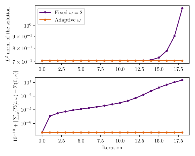
Figure 3: Norm of the solution (top) and difference between the total microscopic entropy at time zero and eventually in time (bottom), when simulating the Burgers equation with and without entropy conservation during the relaxation. In the bottom plot, we add $10^{-10}$ to avoid taking the logarithm of zero.

Let us point out a practical yet fundamental point on the computation of a solution to (22). Indeed, we can have $\bm{f}_{k}\approx\bm{f}_{k}^{\textnormal{eq}}$, thus making $\Delta\Sigma_{(\bm{f}_{1},\dots,\bm{f}_{q})}(\omega)$ quite close to zero with almost zero derivative in $\omega$. This frequently cause issues when iterative methods (Newton, dichotomy, etc.) are employed to solve (22). The idea is to factorize the distance from the equilibrium in the problem: $\Delta\Sigma_{({f}_{+},{f}_{-})}(\omega)=(f_{+}-f_{+}^{\textnormal{eq}})\Delta\tilde{\Sigma}_{({f}_{+},{f}_{-})}(\omega)=0$, so that one eventually solves $\Delta\tilde{\Sigma}_{({f}_{+},{f}_{-})}(\omega)=0$.

Table 4: Errors and order of convergence in the $L^{2}$ norm for the Burgers equation using (22).

$\Delta x$	$L^{2}$ error	Order
2.000E-03	3.725E-06
1.250E-03	1.764E-06	1.59
7.813E-04	1.965E-07	4.67
4.883E-04	3.826E-08	3.48
3.053E-04	5.898E-09	3.98
1.908E-04	9.914E-10	3.79
1.193E-04	1.390E-10	4.18
7.454E-05	2.410E-11	3.73

Finally, we check that the entropy conservation procedure (22) does not change the fourth-order convergence of the method. We operate in the very same setting as in Section 3.1, also re-establishing $V=1.2$. The results in Table 4 confirm that no order reduction is experienced and the scheme retains fourth-order accuracy, as claimed.

5.2 Non-linear system: Shallow water system in 1D

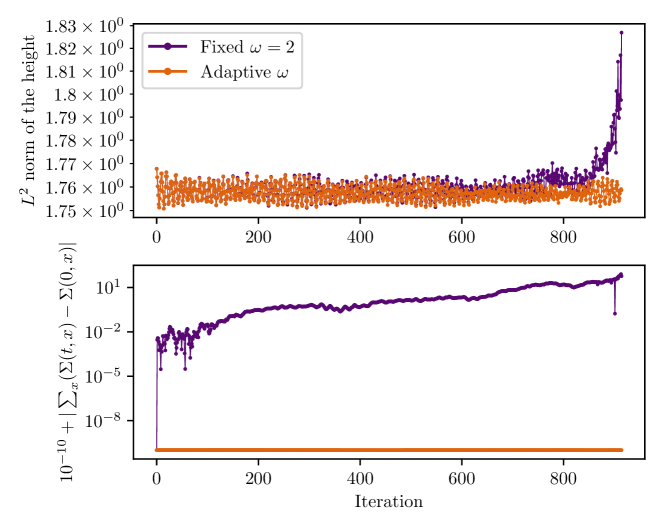
Figure 4: Norm of the solution (height, top) and difference between the total microscopic entropy at time zero and eventually in time (bottom), when simulating the shallow water equations with and without entropy conservation during the relaxation. In the bottom plot, we add $10^{-10}$ to avoid taking the logarithm of zero.

For testing the entropy correction on the shallow water system with gravity $g=1$, we take the initial datum

$$(h,u)(t=0,x)=\begin{cases}(2,0),\qquad&x<1/2,\\ (3/2,0),\qquad&x\geq 1/2,\end{cases}$$

and the kinetic velocity $V=6$ with a spatial grid made up of 100 points. The results are given in Figure 4, where problem (22) has been solved using a quasi-Newton method. This confirms the stabilizing power of the entropy conservation procedure and highlights—once again—that the growth of the total microscopic entropy makes solutions eventually diverge in time.

6 Variations on the numerical scheme and additional numerical experiments

We now propose variations on the basic fourth-order numerical scheme that we have proposed—whose interest will be justified—and additional numerical experiments.

6.1 Projections on the equilibrium

We consider different schemes—where we introduce projections on the equilibrium at different stages. This way of proceeding can be used to reduce oscillations and enhance stability when shocks form. Somehow, these projections can help the numerical scheme to decrease entropy. Before proceeding, notice that $\bm{\mathsf{R}}_{\omega=1}$ is the projection on the equilibrium. The name “projection” perfectly fits for $\bm{\mathsf{R}}_{\omega=1}\bm{\mathsf{R}}_{\omega=1}=\bm{\mathsf{R}}_{\omega=1}$. We consider

Scheme (I) $$\begin{cases}\bm{\phi}(\Delta t)\text{ by \eqref{eq:splittingToUse}},\\ \bm{\psi}(\Delta t)\text{ by \eqref{eq:basicBrickSplitting}}.\end{cases}$$

Scheme (II) $$\begin{cases}\bm{\phi}(\Delta t)=\bm{\mathsf{R}}_{\omega=1}\bm{\psi}\bigl{(}\frac{\Delta t}{6}\bigr{)}^{4}\bm{\psi}\bigl{(}-\frac{\Delta t}{3}\bigr{)}\bm{\psi}\bigl{(}\frac{\Delta t}{6}\bigr{)}^{4},\\ \bm{\psi}(\Delta t)\text{ by \eqref{eq:basicBrickSplitting}}.\end{cases}$$

Scheme (III) $$\begin{cases}\bm{\phi}(\Delta t)=\bigl{(}\bm{\mathsf{R}}_{\omega=1}\bm{\psi}\bigl{(}\frac{\Delta t}{6}\bigr{)}\bigl{)}^{4}\bm{\mathsf{R}}_{\omega=1}\bm{\psi}\bigl{(}-\frac{\Delta t}{3}\bigr{)}\bigl{(}\bm{\mathsf{R}}_{\omega=1}\bm{\psi}\bigl{(}\frac{\Delta t}{6}\bigr{)}\bigl{)}^{4},\\ \bm{\psi}(\Delta t)\text{ by \eqref{eq:basicBrickSplitting}}.\end{cases}$$

Scheme (IV) $$\begin{cases}\bm{\phi}(\Delta t)\text{ by \eqref{eq:splittingToUse}},\\ \bm{\psi}(\Delta t)=\bm{\mathsf{R}}_{\omega=1}\bm{\mathsf{T}}\bigl{(}\frac{\Delta t}{4}\bigr{)}\bm{\mathsf{R}}_{\omega=2}\bm{\mathsf{T}}\bigl{(}\frac{\Delta t}{4}\bigr{)}\bm{\mathsf{R}}_{\omega=1}\bm{\mathsf{T}}\bigl{(}\frac{\Delta t}{4}\bigr{)}\bm{\mathsf{R}}_{\omega=2}\bm{\mathsf{T}}\bigl{(}\frac{\Delta t}{4}\bigr{)}.\end{cases}$$

Let us briefly comment on these schemes. The first one is the original fourth order scheme we have proposed. For Scheme (I), (II), and (III), the basic brick $\bm{\psi}$ is left unchanged. Scheme (II) just performs a projection on the equilibrium at the end of each fourth-order solver. Scheme (III) does so after each employ of the basic brick $\bm{\psi}$. Finally, Scheme (IV) acts in a radically different fashion, for it combines a modified basic brick $\bm{\psi}$ with the same composition. The basic brick $\bm{\psi}$ is modified as a pairing of two Strang formulæ followed by projections on the equilibrium.

6.2 Non-linear scalar problem: Burgers equation in 1D

Table 5: Errors and order of convergence in the $L^{2}$ norm for the Burgers equation using different variation on our new fourth-order scheme.

	Scheme (I)		Scheme (II)		Scheme (III)		Scheme (IV)
$\Delta x$	$L^{2}$ error	Order	$L^{2}$ error	Order	$L^{2}$ error	Order	$L^{2}$ error	Order
Initial datum at equilibrium
2.000E-03	3.370E-06		3.374E-06		3.246E-06		1.147E-05
1.250E-03	1.552E-06	1.65	1.551E-06	1.65	1.476E-06	1.68	5.686E-06	1.49
7.813E-04	1.742E-07	4.65	1.742E-07	4.65	1.677E-07	4.63	1.193E-06	3.32
4.883E-04	3.365E-08	3.50	3.365E-08	3.50	3.275E-08	3.47	3.471E-07	2.63
3.053E-04	5.184E-09	3.98	5.184E-09	3.98	5.091E-09	3.96	8.691E-08	2.95
1.908E-04	8.688E-10	3.80	8.688E-10	3.80	8.586E-10	3.79	2.283E-08	2.84
1.193E-04	1.221E-10	4.18	1.221E-10	4.18	1.212E-10	4.17	5.327E-09	3.10
7.454E-05	2.109E-11	3.74	2.109E-11	3.74	2.099E-11	3.73	1.418E-09	2.82
Initial datum off-equilibrium
2.000E-03	6.432E-06		5.355E-06		4.115E-05		1.653E-04
1.250E-03	1.800E-06	2.71	1.639E-06	2.52	1.069E-05	2.87	6.785E-05	1.90
7.813E-04	2.182E-07	4.49	1.825E-07	4.67	2.576E-06	3.03	2.579E-05	2.06
4.883E-04	3.945E-08	3.64	3.425E-08	3.56	6.346E-07	2.98	1.015E-05	1.98
3.053E-04	6.061E-09	3.99	5.234E-09	4.00	1.551E-07	3.00	3.958E-06	2.00
1.908E-04	9.954E-10	3.84	8.730E-10	3.81	3.796E-08	3.00	1.551E-06	1.99
1.193E-04	1.423E-10	4.14	1.225E-10	4.18	9.245E-09	3.01	6.033E-07	2.01
7.454E-05	2.396E-11	3.79	2.112E-11	3.74	2.264E-09	2.99	2.369E-07	1.99

To start testing the four different schemes proposed hitherto, we consider exactly the same setting as Section 3.1 and we shall test both by initializing the distribution functions at equilibrium and off-equilibrium. The results are given in Table 5 and show fourth-order convergence—when the initial datum is taken at equilibrium—for all numerical schemes except the last one, where order is reduced to three because of the projection on the equilibrium in the basic brick $\bm{\psi}$. Therefore, it is not advisable to employ Scheme (IV). By trying not to initialize at equilibrium, by taking $(f_{+},f_{-})(t=0)=(\tfrac{1}{4},\tfrac{3}{4})u(t=0)$, we observe fourth-order convergence for the first two schemes, third-order for the third scheme, and second-order for the last one, this phenomenon will be explained in a moment. We deduce that Scheme (III) needs to be used carefully, in particular, initializing at equilibrium.

In this non-linear case, the order reduction induced by the projections on the equilibrium could be seen using the modified equations [36, 24] but this would lead to very tedious calculations. Alternatively, this phenomenon can be easily understood in the case of linear transport, where $\varphi(u)=au$, using Fourier analysis [35]. In this case, we can look at the expansions of the two roots $z_{1}$ and $z_{2}$ of $\text{det}(z\bm{\mathsf{Id}}-\hat{\bm{\phi}}(\Delta t)(\xi\Delta x))$ in the limit $|\xi\Delta x|\ll 1$, to theoretically understand the different convergence rates. This provides

$$\text{Scheme (I)}\\ z_{1}(\xi\Delta x)=e^{-ia\xi\Delta t}+\frac{ia}{622080}(24a^{4}-25a^{2}V^{2}+V^{4})(\xi\Delta t)^{5}+\mathcal{O}(|\xi\Delta t|^{6}),\\ z_{2}(\xi\Delta x)\neq 0.$$

$$\text{Scheme (II)}\\ z_{1}(\xi\Delta x)=e^{-ia\xi\Delta t}+\frac{ia}{622080}(24a^{4}-25a^{2}V^{2}+V^{4})(\xi\Delta t)^{5}+\mathcal{O}(|\xi\Delta t|^{6}),\\ z_{2}(\xi\Delta x)=0.$$

$$\text{Scheme (III)}\\ z_{1}(\xi\Delta x)=e^{-ia\xi\Delta t}+\frac{ia}{622080}(24a^{4}-25a^{2}V^{2}+V^{4})(\xi\Delta t)^{5}+\mathcal{O}(|\xi\Delta t|^{6}),\\ z_{2}(\xi\Delta x)=0.$$

$$\text{Scheme (IV)}\\ z_{1}(\xi\Delta x)=e^{-ia\xi\Delta t}+\frac{a^{2}}{3456}(a^{2}-V^{2})(\xi\Delta t)^{4}+\mathcal{O}(|\xi\Delta t|^{5}),\\ z_{2}(\xi\Delta x)=0.$$

We see that only the first scheme allows two discrete modes in the system, because no relaxation on the equilibrium is performed. Moreover, as all the leading order reminders vanish whenever $a=V$ and typically increase with $V$, these expansions suggest that one should take $V\raisebox{-3.69899pt}{\leavevmode\nobreak\ \shortstack{$>$ \\ [-0.07cm]$\sim$}}\leavevmode\nobreak\ a$ but as close as possible to the velocity of the fastest wave, cf. (17), in order to minimize the truncation errors. Notice that in the first three schemes, we could observe fifth-order results provided that $|a|=\sqrt{6}/12V<V$. Indeed, we have even more: since $z_{1}(\xi\Delta x)=e^{-ia\xi\Delta t}+\tfrac{ia}{622080}(24a^{4}-25a^{2}V^{2}+V^{4})(\xi\Delta t)^{5}+\tfrac{a^{2}}{622080}(24a^{4}-25a^{2}V^{2}+V^{4})(\xi\Delta t)^{6}+\mathcal{O}(|\xi\Delta t|^{7})$ in the case of Schemes (I) and (II), the method can be sixth-order and this is what we observe through simulations. For Scheme (III), we have $z_{1}(\xi\Delta x)=e^{-ia\xi\Delta t}+\tfrac{ia}{622080}(24a^{4}-25a^{2}V^{2}+V^{4})(\xi\Delta t)^{5}+\frac{a^{2}}{1244160}(63a^{4}-65a^{2}V^{2}+2V^{4})(\xi\Delta t)^{6}+\mathcal{O}(|\xi\Delta t|^{7})$, hence the scheme remains only fifth-order accurate when $|a|=\sqrt{6}/12V$.

Table 6: Errors and order of convergence in the $L^{2}$ norm for the transport equation with $|a|=\sqrt{6}/12V$ and initial datum at equilibrium.

	Scheme (I)		Scheme (II)		Scheme (III)		Scheme (IV)
$\Delta x$	$L^{2}$ error	Order	$L^{2}$ error	Order	$L^{2}$ error	Order	$L^{2}$ error	Order
5.000E-02	2.283E-02		2.283E-02		2.307E-02		1.591E-01
3.125E-02	1.890E-03	5.30	1.890E-03	5.30	2.660E-03	4.60	5.120E-02	2.41
1.961E-02	1.239E-04	5.85	1.239E-04	5.85	2.662E-04	4.94	1.321E-02	2.91
1.235E-02	8.066E-06	5.90	8.066E-06	5.90	2.713E-05	4.94	3.394E-03	2.94
7.752E-03	5.040E-07	5.96	5.040E-07	5.96	2.685E-06	4.97	8.506E-04	2.97
4.854E-03	3.081E-08	5.97	3.081E-08	5.97	2.616E-07	4.98	2.111E-04	2.98
3.040E-03	1.855E-09	6.00	1.855E-09	6.00	2.514E-08	5.00	5.171E-05	3.00
1.901E-03	1.111E-10	6.00	1.111E-10	6.00	2.406E-09	5.00	1.265E-05	3.00

These predictions are actually met by the results of Table 6. They are obtained exactly in the same setting as for the Burgers equation, taking a final time $T=10$ and quite coarse meshes in order to avoid very small errors below machine epsilon in double precision, since the numerical methods are now extremely accurate. Of course, this is of limited interest since valid only in the linear setting and does not extend to the case of the Burgers equation. However, a similar idea could be utilized in the simulation of low-Mach–flows, where the wave speed is roughly constant in the domain, in order to obtain, if not sixth-order schemes, very accurate fourth-order ones.

To understand the order reductions experienced when the initial datum is not at equilibrium, cf. bottom half of Table 5, again in the linear setting, we follow the procedure by [7], which has allowed to explain the behavior of the standard second-order lattice Boltzmann scheme as far as initializations are concerned. Considering that $(f_{+},f_{-})(t=0)=(\theta,1-\theta)u(t=0)$ with $\theta\in\mathbb{R}$, we study the low-frequency limit of $\hat{\mathsf{g}}(\xi\Delta x)=(\bm{e}_{1}^{T}+\bm{e}_{2}^{T})\hat{\bm{\phi}}(\Delta t)(\xi\Delta x)(\theta,1-\theta)^{T}$, the amplification factor giving the approximation of the conserved variable $u$ after one time step, as function of the initial datum of the Cauchy problem. We have

$$\textnormal{Scheme (I) and (II)}\qquad\hat{\mathsf{g}}(\xi\Delta x)=e^{-ia\xi\Delta t}+\mathcal{O}(|\xi\Delta t|^{5}),$$

independently of $\theta$, which explains why fourth-order is indeed kept. For the other schemes

$$\textnormal{Scheme (III)}\qquad\hat{\mathsf{g}}(\xi\Delta x)=e^{-ia\xi\Delta t}-\frac{ia^{2}}{1728}(a+V-2V\theta)(\xi\Delta t)^{3}+\mathcal{O}(|\xi\Delta t|^{4}),$$

hence we understand why we observe third-order convergence except when the initial datum is at equilibrium, that is $\theta=\tfrac{1}{2}(1+\tfrac{a}{V})$. Finally, we have

$$\textnormal{Scheme (IV)}\qquad\hat{\mathsf{g}}(\xi\Delta x)=e^{-ia\xi\Delta t}+\frac{a}{288}(a+V-2V\theta)(\xi\Delta t)^{2}+\mathcal{O}(|\xi\Delta t|^{3}),$$

yielding the same conclusion at second-order.

6.3 Solution of the Euler equations in 2D with Riemann problems

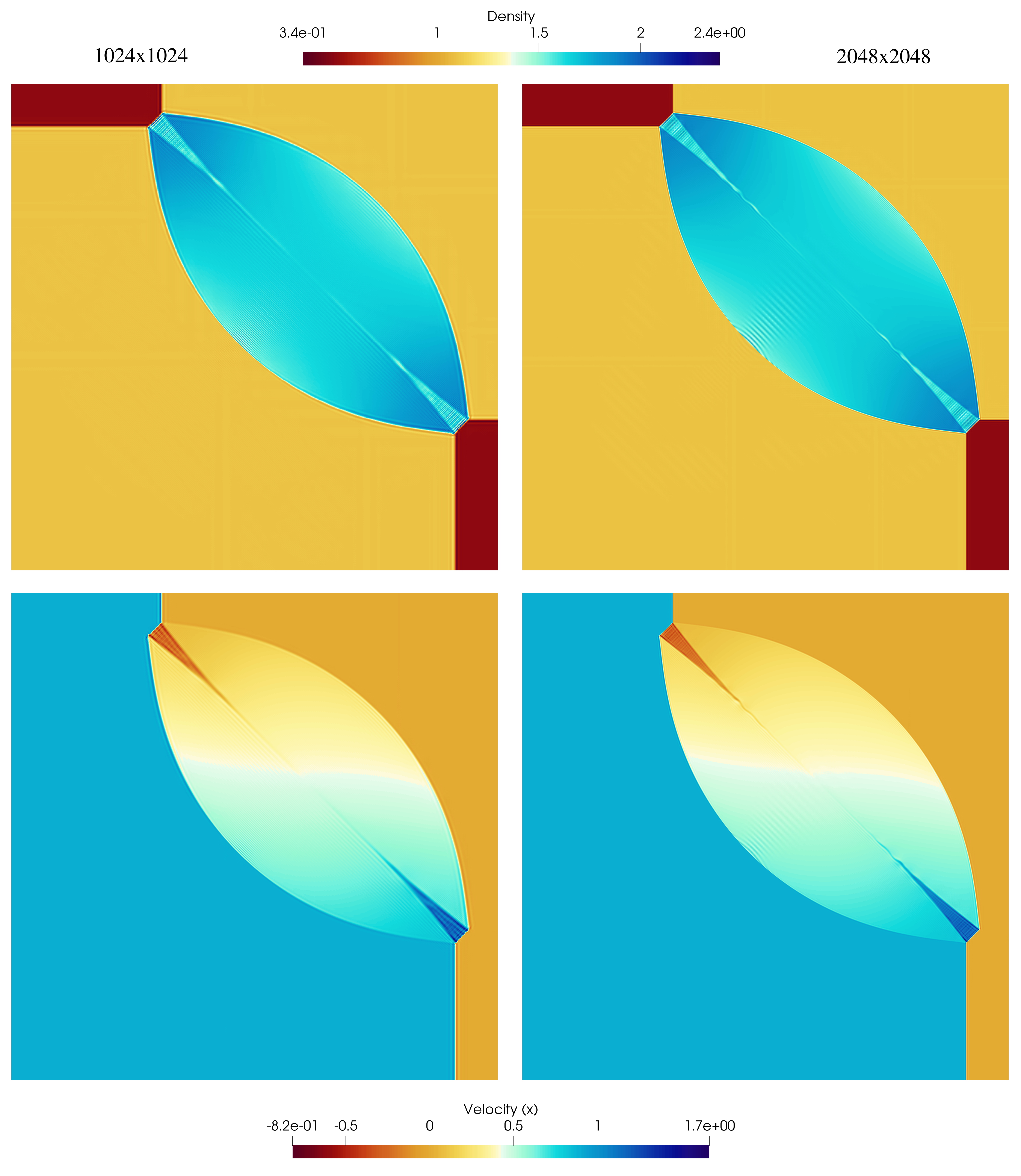
Figure 5: Density and velocity along $x$ at final time $T=0.25$ with Riemann problems for the Euler equations, using Configuration 4 from [31] and employing Scheme (III).

We finish the paper on a test concerning the full Euler system in 2D with discontinuous solutions. Therefore, we have $d=2$, $M=4$ with $\bm{u}=(u_{1},u_{2},u_{3},u_{4})=(\rho,\rho u,\rho v,E)$ under the fluxes $\bm{\varphi}^{1}(\rho,u,v,p)=(\rho u,\rho u^{2}+p,\rho uv,u(E+p))$ and $\bm{\varphi}^{2}(\rho,u,v,p)=(\rho v,\rho uv,\rho v^{2}+p,v(E+p))$, where the link between energy $E$ and pressure $p$ is given by the polytropic equation of state

$$E=\frac{1}{2}\rho(u^{2}+v^{2})+\frac{p}{\gamma-1},$$

with $\gamma$ the gas constant.

We consider an initial datum made up of a Riemann problem with four constant states, given by the configuration 4 from [31], with gas constant $\gamma=1.4$. The grids are made up of 1024 and 2048 points per direction, with a kinetic velocity $V=6.21$. We are able to use $\omega=2$, hence making the scheme fourth-order accurate, provided that we employ Scheme (III). Indeed, the projection on the equilibrium at each call of the basic brick $\bm{\psi}$ has a very positive effect on stability. Notice that one could add shock detection algorithms in order to set $\omega=2$ far from shocks and $\omega$ slightly smaller than two, ensuring the elimination of spurious oscillations. However, as claimed at the very beginning of the manuscript, this is beyond the proof-of-concept status of the paper and shall not be investigated here. The simulations are not stable when using Scheme (I) and $\omega=2$. After $T=0.25$, the density field is plotted in Figure 5. This result is in agreement with [31] and we start to observe, when using 2048 points per direction, hydrodynamic instabilities along the central axis of the almond-shaped structure. This indicates that the underlying numerical scheme is a high-order one.

7 Conclusions

In this study, we have introduced a general framework for constructing fourth-order lattice Boltzmann schemes tailored to handle hyperbolic systems of conservation laws. Our procedure relies on time-symmetric operators, combined together to increase the order of the method. For we employ a kinetic relaxation approximation, we can adjust the kinetic velocities to ensure that the resulting scheme adheres to the lattice Boltzmann method principles. Numerical simulations have been conducted to validate our theoretical findings. Furthermore, we have proposed modifications to the local relaxation phase to maintain entropy stability without compromising the order of the method.

Future research directions include the development of limitation strategies—both a priori and a posteriori—for these lattice Boltzmann schemes to effectively address numerical oscillations arising from shocks. Additionally, techniques to ensure positivity, particularly when dealing with shallow water equations, will be of interest. Finally, exploring methods to further increase the order of the scheme, potentially up to six or beyond, holds promise for enhancing accuracy and computational efficiency.

References

- [1] R. Abgrall and F. Nassajian Mojarrad, An arbitrarily high order and asymptotic preserving kinetic scheme in compressible fluid dynamic, Communications on Applied Mathematics and Computation, (2023), pp. 1–29.
- [2] D. Aregba-Driollet and R. Natalini, Discrete kinetic schemes for multidimensional systems of conservation laws, SIAM Journal on Numerical Analysis, 37 (2000), pp. 1973–2004.
- [3] M. Atif, P. K. Kolluru, C. Thantanapally, and S. Ansumali, Essentially entropic lattice Boltzmann model, Physical Review Letters, 119 (2017), p. 240602.
- [4] H. Baty, F. Drui, P. Helluy, E. Franck, C. Klingenberg, and L. Thanhäuser, A robust and efficient solver based on kinetic schemes for Magnetohydrodynamics (MHD) equations., Applied Mathematics and Computation, 440 (2023), p. 127667, https://doi.org/10.1016/j.amc.2022.127667, https://hal.science/hal-02965967.
- [5] T. Bellotti, The influence of parasitic modes on “weakly” unstable multi-step Finite Difference schemes, arXiv preprint arXiv:2312.14503, (2023).
- [6] T. Bellotti, Truncation errors and modified equations for the lattice Boltzmann method via the corresponding Finite Difference schemes, ESAIM: Mathematical Modelling and Numerical Analysis, 57 (2023), pp. 1225–1255.
- [7] T. Bellotti, Initialisation from lattice Boltzmann to multi-step Finite Difference methods: modified equations and discrete observability, Journal of Computational Physics, 504 (2024), p. 112871.
- [8] T. Bellotti, L. Gouarin, B. Graille, and M. Massot, Multidimensional fully adaptive lattice Boltzmann methods with error control based on multiresolution analysis, Journal of Computational Physics, 471 (2022), p. 111670.
- [9] T. Bellotti, L. Gouarin, B. Graille, and M. Massot, Multiresolution-based mesh adaptation and error control for lattice Boltzmann methods with applications to hyperbolic conservation laws, SIAM Journal on Scientific Computing, 44 (2022), pp. A2599–A2627.
- [10] F. Bouchut, Construction of BGK models with a family of kinetic entropies for a given system of conservation laws, Journal of Statistical Physics, 95 (1999), pp. 113–170.
- [11] F. Bouchut, Entropy satisfying flux vector splittings and kinetic BGK models, Numerische Mathematik, 94 (2003), pp. 623–672.
- [12] F. Bouchut, Nonlinear Stability of Finite Volume Methods for Hyperbolic Conservation Laws and Well-Balanced schemes for Sources, Springer Science & Business Media, 2004.
- [13] R. Brownlee, A. N. Gorban, and J. Levesley, Stability and stabilization of the lattice Boltzmann method, Physical Review E, 75 (2007), p. 036711.
- [14] Y. Chen, Z. Chai, and B. Shi, Fourth-order multiple-relaxation-time lattice Boltzmann model and equivalent finite-difference scheme for one-dimensional convection-diffusion equations, Physical Review E, 107 (2023), p. 055305.
- [15] D. Coulette, E. Franck, P. Helluy, M. Mehrenberger, and L. Navoret, High-order implicit palindromic discontinuous Galerkin method for kinetic-relaxation approximation, Computers & Fluids, 190 (2019), pp. 485–502.
- [16] P. J. Dellar, An interpretation and derivation of the lattice Boltzmann method using Strang splitting, Computers & Mathematics with Applications, 65 (2013), pp. 129–141.
- [17] F. Drui, E. Franck, P. Helluy, and L. Navoret, An analysis of over-relaxation in a kinetic approximation of systems of conservation laws, Comptes Rendus Mécanique, 347 (2019), pp. 259–269.
- [18] F. Dubois, Stable lattice Boltzmann schemes with a dual entropy approach for monodimensional nonlinear waves, Computers & Mathematics with Applications, 65 (2013), pp. 142–159.
- [19] F. Dubois, Simulation of strong nonlinear waves with vectorial lattice Boltzmann schemes, International Journal of Modern Physics C, 25 (2014), p. 1441014.
- [20] F. Dubois, Nonlinear fourth order Taylor expansion of lattice Boltzmann schemes, Asymptotic Analysis, 127 (2022), pp. 297–337.
- [21] T. Février, Extension et analyse des schémas de Boltzmann sur réseau : les schémas à vitesse relative, theses, Université Paris Sud - Paris XI, Dec. 2014, https://theses.hal.science/tel-01126994.
- [22] E. Godlewski and P.-A. Raviart, Numerical approximation of hyperbolic systems of conservation laws, vol. 118, Springer Science & Business Media, 2013.
- [23] B. Graille, Approximation of mono-dimensional hyperbolic systems: A lattice Boltzmann scheme as a relaxation method, Journal of Computational Physics, 266 (2014), pp. 74–88.
- [24] K. Guillon, R. Hélie, and P. Helluy, Stability analysis of the vectorial lattice-Boltzmann method. working paper or preprint, Feb. 2023, https://hal.science/hal-03986533.
- [25] F. J. Higuera and J. Jiménez, Boltzmann approach to lattice gas simulations, Europhysics Letters, 9 (1989), p. 663.
- [26] S. A. Hosseini, M. Atif, S. Ansumali, and I. V. Karlin, Entropic lattice Boltzmann methods: A review, Computers & Fluids, (2023), p. 105884.
- [27] S. Jin and Z. Xin, The relaxation schemes for systems of conservation laws in arbitrary space dimensions, Communications on Pure and Applied Mathematics, 48 (1995), pp. 235–276.
- [28] M. Junk and W.-A. Yong, Weighted -Stability of the Lattice Boltzmann Method, SIAM Journal on Numerical Analysis, 47 (2009), pp. 1651–1665.
- [29] P. Lafitte, W. Melis, and G. Samaey, A high-order relaxation method with projective integration for solving nonlinear systems of hyperbolic conservation laws, Journal of Computational Physics, 340 (2017), pp. 1–25.
- [30] P. Lallemand and L.-S. Luo, Theory of the lattice Boltzmann method: Dispersion, dissipation, isotropy, Galilean invariance, and stability, Physical Review E, 61 (2000), p. 6546.
- [31] P. D. Lax and X.-D. Liu, Solution of two-dimensional Riemann problems of gas dynamics by positive schemes, SIAM Journal on Scientific Computing, 19 (1998), pp. 319–340.
- [32] R. I. McLachlan and G. R. W. Quispel, Splitting methods, Acta Numerica, 11 (2002), pp. 341–434.
- [33] J. J. Miller, On the location of zeros of certain classes of polynomials with applications to numerical analysis, IMA Journal of Applied Mathematics, 8 (1971), pp. 397–406.
- [34] R. T. Rockafellar, Convex Analysis, Princeton University Press, Princeton, 1970, https://doi.org/doi:10.1515/9781400873173, https://doi.org/10.1515/9781400873173.
- [35] J. C. Strikwerda, Finite difference schemes and partial differential equations, SIAM, 2004.
- [36] R. F. Warming and B. Hyett, The modified equation approach to the stability and accuracy analysis of finite-difference methods, Journal of Computational Physics, 14 (1974), pp. 159–179.