Optimal VPPI strategy under Omega ratio with stochastic benchmark

Abstract

This paper studies a variable proportion portfolio insurance (VPPI) strategy. The objective is to determine the risk multiplier by maximizing the extended Omega ratio of the investor’s cushion, using a binary stochastic benchmark. When the stock index declines, investors aim to maintain the minimum guarantee. Conversely, when the stock index rises, investors seek to track some excess returns. The optimization problem involves the combination of a non-concave objective function with a stochastic benchmark, which is effectively solved based on the stochastic version of concavification technique. We derive semi-analytical solutions for the optimal risk multiplier, and the value functions are categorized into three distinct cases. Intriguingly, the classification criteria are determined by the relationship between the optimal risky multiplier in Zieling et al., (2014) and the value of $1$. Simulation results confirm the effectiveness of the VPPI strategy when applied to real market data calibrations.

Keywords: VPPI; Omega ratio; Stochastic benchmark; Risk multiplier; Concavification. JEL Classifications: G11, C60, C61.

1 Introduction

Risk-averse investors adopt portfolio insurance strategies to manage downside risk while capturing part of the stock market flourish. The original idea, introduced by Leland, (1980), is known as the option-based portfolio insurance (OBPI) strategy. Subsequently, Black and Jones, (1987) proposed the constant proportion portfolio insurance (CPPI) strategy, which not only matches the performance of OBPI but also offers a more straightforward implementation. CPPI involves dynamically adjusting the asset allocation in the portfolio based on a pre-determined formula, which typically involves a combination of risky assets (such as stocks) and safer assets (such as bonds or cash). Researchers and practitioners in the field of asset management have extensively studied and applied CPPI, with numerous studies delving into various aspects of dynamic portfolio insurance. For instance, refer to Bertrand and Prigent, (2001); Chen et al., (2008); Schied, (2014); Hambardzumyan and Korn, (2019), among others.

The risk multiplier plays a pivotal role in CPPI strategies, influencing both portfolio leverage and performance. The proportion invested in the risky asset is determined by multiplying the cushion with the risk multiplier. Traditionally, the risk multiplier has been considered fixed and predetermined. However, during periods of heightened market volatility, a substantial risk multiplier can lead to significant losses. Consequently, incorporating a time-varying risk multiplier can enhance performance. This flexibility allows investors to adjust their risk exposure in response to evolving market conditions. As a result, variable proportion portfolio insurance (VPPI) strategies have garnered extensive attention, falling into two categories: parametric optimization and non-parametric optimization. In the context of parametric optimization, Zieling et al., (2014) introduced an optimization model for the risk multiplier for investors exhibiting hyperbolic absolute risk aversion (HARA) preference. The research findings suggest that the risk multiplier is influenced by the Sharpe ratio of the risky asset and the risk-averse attitude of the investor. Schied, (2014) concerned a dynamic extension of the CPPI strategy in which the multiplier level may depend on quantities including time and price evolution. Similarly, Bertrand and Prigent, (2016) employed extreme value theory to establish an upper bound for the risk multiplier. Dichtl and Drobetz, (2011) explored the incorporation of cumulative prospect theory to capture the heterogeneous attitudes of investors towards gain and loss within the VPPI framework. Ameur and Prigent, (2014) assumed that the risk multiplier is determined from market and portfolio dynamics. For non-parametric optimization, Cesari and Cremonini, (2003) integrated technical predictions, such as the 10-week moving average, into the strategy design. Additionally, statistical and machine learning methods have been employed in the design of the risk multiplier see Chen et al., (2008); Lee et al., (2008); Dehghanpour and Esfahanipour, (2017), etc. All of these researches have demonstrated improved performance of VPPI strategies compared to standard CPPI strategies. This paper adopts a parametric modeling approach, aiming to identify the optimal risk multiplier based on appropriate optimization objectives.

This paper aims to determine the optimal VPPI strategy based on a specific criterion. In the literature, various approaches have been used to optimize utility or maximize returns for a given level of risk. In Zieling et al., (2014), the HARA utility function is optimized to find the optimal risk multiplier for CPPI strategies. Another commonly applied criterion in economics is maximizing the expected return while considering a certain level of risk. The Sharpe ratio, which quantifies the trade-off between risk and reward using variance and mean, has been widely used for this purpose. However, it has limitations as it assumes an elliptical distribution of portfolio returns. To address the limitations of the Sharpe ratio, alternative risk measures have been proposed. One such measure is the Omega ratio, introduced in Keating and Shadwick, (2002), which considers the entire return distribution and distinguishes gains and losses from a specified threshold. Unlike the Sharpe ratio, the Omega ratio incorporates both upside and downside deviations and has characteristics of symmetric and asymmetric risk measures. Moreover, the Omega ratio does not assume a specific distribution of portfolio returns and is commonly applied in finance, see Kane et al., (2009); Bertrand and Prigent, (2011); Guastaroba et al., (2016); Biedova and Steblovskaya, (2020), etc. In this paper, we depart from the approach of Zieling et al., (2014) and consider maximizing the Omega ratio of the terminal cushion as the objective for investors. However, it is worth noting that Bernard et al., (2019) states that the maximization problem of the Omega ratio is unbounded in the continuous setting. To address this issue, we extend the Omega ratio following the approach in Lin et al., (2019) to overcome the problem of ill-posedness.

The Omega ratio is a measure that distinguishes gains and losses based on a specified benchmark. However, selecting an appropriate benchmark is not formally guided, as mentioned in Keating and Shadwick, (2002). In the study conducted by Kapsos et al., (2014), it was highlighted that the solution to maximize the Omega ratio is highly sensitive to the chosen benchmark. This poses a challenge as financial markets are inherently uncertain and prone to volatility. A deterministic threshold may not adequately capture the randomness and variability of market conditions. To address this issue, researchers have explored the concept of a stochastic benchmark in several studies, such as De Giorgi and Post, (2011), Sprenger, (2015), and He and Strub, (2022), etc. By introducing stochasticity into the benchmark, investors can better account for the unpredictable nature of asset returns and ensure a more realistic assessment of gains and losses. In the field of asset management, investors typically aim for upside capture and downside protection, often relying on a binary benchmark. In other words, when the stock index performs poorly, investors seek to maintain a minimum guarantee. Conversely, when the stock index performs well, investors aim to track some excess returns. Taking these practical considerations into account, we formulate a binary stochastic benchmark to determine the gains and losses in the extended Omega ratio.

The objective function in this context is a non-linear ratio, lacking convexity or concavity. Moreover, the optimization problem is complicated because of stochastic benchmark. These two characteristics combine to create the main challenges faced when attempting to solve this optimization problem. Following the fractional programming method in Dinkelbach, (1967), we transform the original optimization problem into a family of solvable linearized problems in which the objective function is defined as the numerator of the original problem minus the denominator multiplied by a penalty parameter. Remarkably, one of these reformulated problems provides an exact solution to the original problem. Additionally, we employ the martingale method to simplify the problem, transitioning from optimizing over a space of stochastic processes to optimizing over a space of random variables, as exemplified in Karatzas et al., (1998). For objective functions that are not concave, concavification techniques are commonly employed, see Carpenter, (2000); Lin et al., (2019); He and Kou, (2018). In our paper, we tackle the optimization problem that combines a non-concave objective function with a stochastic benchmark. This kind of problem lacks systematic research, and our previous work Liang et al., (2021) investigates an abstract framework regarding this kind of problem and propose a stochastic version of the concavification technique. Applying the results from this work, we derive the semi-analytical optimal risky multiplier and its corresponding value function. Theoretical results indicate that both the guarantee ratio and the capturing ratio exert significant influences on the value functions. When both of these ratios are low, the value function approaches infinity. Under less stringent conditions, the cushion consistently exceeds the benchmark, leaving only room for gains. Conversely, with stricter requirements, the form of the value functions falls into one of three distinct categories. Remarkably, the criteria for this classification are based on the relationship between the optimal risky multiplier as detailed in Zieling et al., (2014) and the value of 1. Furthermore, the optimal risky multiplier exhibits a distinct hump-shaped pattern attributed to the inherent loss aversion attitude of investors. This behavior leads investors to increase their allocation to risky assets as they approach the maturity date, driven by the desire to minimize potential losses and maximize gains through speculative investments. Notably, the optimal risk multiplier tends to be lower compared to the one under the CRRA utility framework. This difference can be attributed to the presence of loss aversion, which promotes a more cautious approach characterized by lower leverage.

While we have successfully derived semi-closed-form solutions within a continuous-time framework, it is imperative to assess the efficacy of these strategies in a discrete-time context. The effectiveness of these strategies in discrete-time scenarios is crucial, as it directly influences their practical applicability (as discussed in Black and Jones, (1987) and Balder et al., (2009)). Specifically, our investment strategy involves adjustments at fixed time intervals, as seen in Branger et al., (2010) and Happersberger et al., (2020), or it may be triggered by reaching specific thresholds, similar to the approach in Weng, (2013). Given that we distinguish between the minimal guarantee and the benchmark, selecting a consistent threshold can be challenging. Therefore, in this paper, we opt for the fixed time interval adjustment mechanism. For comparative analysis, we utilize the fixed multiplier strategy from Zieling et al., (2014) as well as a constant multiplier as benchmarks. Under these settings, we evaluate the effectiveness of the strategy using various criteria, including Omega ratio, guarantee probability, expected terminal excess value, probability of underperformance, and winning probability. These metrics allow for a comprehensive assessment of the strategy’s performance. Our results confirm the effectiveness of the VPPI strategy when applied to real market data calibrations. Furthermore, we observe a negative correlation between the performance of the VPPI strategy and both the required guarantee ratio and the capturing ratio. A higher guarantee (or capturing) ratio reduces the flexibility in investment and increases the difficulty in maintaining the minimal guarantee or tracking the benchmark. It is worth noting that the impact of performance parameters is multifaceted, as they not only affect investment performance but also influence variations in benchmark performance.

The contribution of the paper is threefold. First, we introduce the binary stochastic benchmark and the Omega ratio within the VPPI model, effectively capturing the objectives of investors in the field of asset management. Second, we expand the concavification technique into a stochastic framework, successfully addressing optimization challenges associated with non-concave objective functions and stochastic benchmarks. We establish semi-analytical value functions, categorizing them into three distinct cases. Lastly, our research yields several intriguing findings. We observe that the optimal risk multiplier follows a distinctive hump-shaped pattern and tends to be lower in comparison to fixed multipliers. Furthermore, the VPPI strategy outperforms alternative policies by demonstrating superior tracking of benchmarks and reducing negative gaps. We also elucidate the intricate relationship between expected returns on risky investments and the optimal strategies.

The remainder of the paper is organized as follows. Section 2 provides the mathematical formulation of the investor’s optimization problem with Omega ratio and stochastic benchmark. In Section 3, we use the stochastic version of concavification techniques to solve the optimization problem. Section 4 exhibits the numerical results and the main findings. Finally, we conclude the paper in Section 5.

2 Model Setting

Consider a filtered probability space $(\Omega,\mathcal{F},\{\mathcal{F}_{t}\}_{t\geqslant 0},\mathbb{P})$, where $\mathbb{P}$ is the reference probability measure. Before introducing the VPPI strategy, let us discuss the construction of the CPPI strategy.

The current value of a portfolio at time $t$ is denoted as $V_{t}$, which comprises both the value of the risky asset and the risk-free asset. The floor value, denoted as $F_{t}$, represents the minimum guarantee or downside protection level. The objective of the investor is to ensure that the portfolio value remains above this guarantee. The cushion at time $t$, denoted as $C_{t}$, is defined as the difference between the current portfolio value and the floor value, i.e.,

$$C_{t}=V_{t}-F_{t}.$$

In the CPPI strategy, the risk multiplier, denoted as $m$, is a constant value. The allocation to the risky assets is determined as a proportion of the cushion. Specifically, the investment in risky assets at time $t$ can be calculated by

$$e_{t}=m(V_{t}-F_{t})\triangleq mC_{t}.$$ (2.1)

The remaining portion $(V_{t}-e_{t})$ is allocated to risk-free assets. The CPPI strategy is a straightforward approach that has found wide application in asset allocation. The risk multiplier $m$ plays a crucial role in the CPPI strategy and has been assigned different values in previous research. For instance, $m$ was set to 5 in Herold et al., (2007), 14 in Annaert et al., (2009), and 3 in Zhang et al., (2015). Specifically, Biedova and Steblovskaya, (2020) chose the optimal multiplier value with respect to the Omega ratio in the CPPI strategy.

However, it is important to note that using a constant risk multiplier can have limitations. One such limitation is a lack of flexibility in adapting to changing market conditions. Market volatility and risk levels can fluctuate over time, and a fixed multiplier may not effectively respond to these variations. Additionally, a constant risk multiplier can lead to larger losses during periods of significant market downturns. Setting the multiplier too high could result in a higher allocation to risky assets when market conditions rapidly deteriorate, potentially amplifying losses.

The VPPI strategy addresses the limitations of a constant risk multiplier by employing time-varying multipliers that adjust dynamically based on market conditions. In the VPPI strategy, the constant risk multiplier $m$ is replaced with a square integrable and adaptive process denoted as

$$\{m_{t},t\geqslant 0\}.$$

The value of $m_{t}$ changes over time according to a predefined rule or algorithm, allowing it to capture changes in market conditions and risk levels. In Zieling et al., (2014), the optimal risk multiplier for the VPPI strategy is obtained by maximizing the CRRA utility of the cushion. This approach takes into account investors’ risk preferences and aims to find the risk multiplier that optimizes their utility function. In our work, different from Zieling et al., (2014), we optimize the risk multiplier for the VPPI strategy using the extended Omega ratio. The extended Omega ratio is a risk-adjusted performance measure that considers both downside risk and upside potential. By optimizing the risk multiplier based on this measure, we aim to enhance the risk-adjusted performance of the VPPI strategy.

Similar to Biedova and Steblovskaya, (2020), we consider continuous time rebalancing in the Black-Scholes market. There are two assets in the financial market: a risk-free asset $B$ and a risky asset $S$, which are described as follows:

$$\left\{\begin{aligned} \frac{dB_{t}}{B_{t}}&=rdt,~{}B_{0}=1,\\ \frac{dS_{t}}{S_{t}}&=\mu dt+\sigma dW_{t},~{}S_{0}=1,\end{aligned}\right.$$

where $\{W_{t}:t\geqslant 0\}$ is a standard Brownian motion defined on the filtered probability space $(\Omega,\mathcal{F},\{\mathcal{F}_{t}\}_{t\geqslant 0},\mathbb{P})$. The first equation represents the risk-free asset, with the constant interest rate $r$ representing the risk-free rate of return. The second equation describes the risky asset, with $\mu$ representing the expected return and $\sigma$ representing the volatility of the asset.

Suppose that the investor has an initial value $V_{0}=1$, and the guarantee $F_{t}$ in the VPPI strategy satisfies the equation

$$dF_{t}=rF_{t}dt,~{}F_{0}=kV_{0}=k,$$

where $k$ is the guarantee proportion. The initial guarantee $F_{0}$ is set as a fixed proportion $k$ of the initial portfolio value $V_{0}$. This setup ensures that the guarantee keeps pace with the growth of the risk-free asset and provides a minimum protection level for the portfolio.

In the Omega ratio, as originally proposed by Keating and Shadwick, (2002), the benchmark is traditionally considered as a constant value that distinguishes gains from losses. The benchmark used by the investor is often stochastic and varies according to the prevailing market conditions. Specifically, when the financial market performs well, the investor wants to track a portion of returns exceeding the index. When it performs poorly, the benchmark is set to be 0, i.e., the investor wants to maintain the minimal guarantee. To evaluate the cushion $C_{T}$ of the investor, we introduce a binary benchmark formulated as follows:

$$Y=\left\{\begin{aligned} &0,&S_{T}<F_{T},\\ &\eta(S_{T}-F_{T}),&S_{T}\geqslant F_{T}.\end{aligned}\right.$$ (2.2)

Here $\eta\leqslant 1$ is a multiplier. Our goal is to find the optimal $m$ to maximizing the extended Omega ratio with a binary benchmark:

$$\max\limits_{\{m_{t},0\leqslant t\leqslant T\}}\frac{\mathbb{E}\left[U(C_{T}-Y)\mathds{1}_{\{C_{T}>Y\}}\right]}{\mathbb{E}\left[U(Y-C_{T})\mathds{1}_{\{C_{T}\leqslant Y\}}\right]},$$ (2.3)

where $U(x)=x^{\gamma},\gamma<1$. In Problem (2.3), when $C_{T}$ exceeds $Y$ ($C_{T}$ falls short of $Y$), the investor realizes gains (suffers losses). The investor’s preference is characterized by the attitude towards gains relative to the attitude towards losses. When the parameter $\gamma$ is set to 1, Problem (2.3) represents the standard Omega ratio. However, as noted by Bernard et al., (2019), in the continuous setting, the maximization problem of the Omega ratio becomes unbounded. To address this, we extend the Omega ratio in Problem (2.3) by incorporating the function $U(x)=x^{\gamma}$. This extension has also been explored in Lin et al., (2019).

3 Optimal multiplier

In this section, we focus on deriving the optimal multiplier for Problem (2.3). This problem involves fractional optimization with a stochastic benchmark. Stochastic dynamic programming method cannot be applied. To address it, we initially employ the martingale method, as outlined in Karatzas et al., (1991), and the linearization technique, as described in Lin et al., (2019). These methods allow us to transform Problem (2.3) into a non-concave optimization problem within a space of random variables featuring a stochastic benchmark. Subsequently, we employ the stochastic version of the concavification technique, as proposed in Liang et al., (2021), to tackle and resolve the transformed problem.

3.1 Martingale method

We begin by deriving the dynamics of the cushion, represented as the excess value $C_{t}$. This dynamic is a consequence of (2.1), and it follows that

$$\begin{split}dC_{t}&=dV_{t}-dF_{t}=(V_{t}-e_{t})\frac{dB_{t}}{B_{t}}+e_{t}\frac{dS_{t}}{S_{t}}-dF_{t}\\ &=(C_{t}+F_{t}-m_{t}C_{t})rdt+m_{t}C_{t}\frac{dS_{t}}{S_{t}}-rF_{t}dt\\ &=(C_{t}-m_{t}C_{t})rdt+m_{t}C_{t}\frac{dS_{t}}{S_{t}}\\ &=\left[m_{t}(\mu-r)+r\right]C_{t}dt+m_{t}\sigma C_{t}dW_{t},\end{split}$$ (3.1)

and $C_{0}=V_{0}-kV_{0}=1-k$. Based on (3.1), we can employ the martingale method, as described in Karatzas et al., (1991) and Cox and Huang, (1989), to transform the original problem into the following optimization problem concerning the terminal cushion:

$$\sup_{C_{T}\in\mathcal{C}}~{}\frac{\mathbb{E}\left[U(C_{T}-Y)\mathds{1}_{\{C_{T}>Y\}}\right]}{\mathbb{E}\left[U(Y-C_{T})\mathds{1}_{\{C_{T}\leqslant Y\}}\right]}$$ (3.2)

with budget constraint

$$\mathcal{C}=\left\{C_{T}~{}\text{is nonnegative and }\mathcal{F}_{T}\text{-measurable}~{}\bigg{|}~{}\mathbb{E}\left[\xi_{T}C_{T}\right]\leqslant 1-k\right\},$$ (3.3)

where $\xi_{t}=\exp\left\{-rt-\frac{\theta^{2}}{2}t-\theta W_{t}\right\}$ is the pricing kernel with $0\leqslant t\leqslant T$ and $\theta=\frac{\mu-r}{\sigma}$.

3.2 Linearization

The objective function in Problem (3.2) is a fractional form, which cannot be solved directly. To address this, we utilize fractional programming theory and introduce a family of linearized problems. This family of problems is parameterized by a non-negative factor $\lambda$, as described in Lin et al., (2019):

$$f(\lambda)=\sup_{C_{T}\in\mathcal{C}}~{}\left\{\mathbb{E}\left[U(C_{T}-Y)\mathds{1}_{\{C_{T}>Y\}}\right]-\lambda\mathbb{E}\left[U(Y-C_{T})\mathds{1}_{\{C_{T}\leqslant Y\}}\right]\right\}.$$ (3.4)

By linearizing the original fractional objective function, we transform the problem into a set of linearized problems. We have the following proposition on relationship between $f(\cdot)$ in Problem (3.4) and the optimal solution to Problem (3.2):

Proposition 1.

Assume $1-k<\mathbb{E}[\xi_{T}Y]$, then $f(\cdot)$ has a zero point $\lambda^{*}$. If the optimization problem (3.4) with $\lambda$ being $\lambda^{*}$ has an optimal solution $C_{T}^{*}$, then $C_{T}^{*}$ is also an optimal solution for Problem (3.2), and $\lambda^{*}$ is the unique value function of Problem (3.2).

Proof.

See Appendix A. ∎

Remark 1.

Note that if $1-k\geqslant\mathbb{E}[\xi_{T}Y]$, then one can find a $C_{T}\in\mathcal{C}$ such that $C_{T}\geqslant Y$ a.s., which leads to a zero term in the denominator of Problem (3.2), and the problem is meaningless. This indicates that the benchmark $Y$ should not be set too small relative to the guarantee level $k$.

3.3 Solution to the linearized probelm

Proposition 1 suggests that to solve the original problem (3.2), it is sufficient to find solutions to the linearized problem (3.4). Rewrite Problem (3.4) as

$$f(\lambda)=\sup_{C_{T}\in\mathcal{C}}~{}\mathbb{E}\left[u_{\lambda}(C_{T},Y)\right],$$ (3.5)

where $u_{\lambda}$ is defined as

$$u_{\lambda}(c,y)=\left\{\begin{aligned} &(c-y)^{\gamma},&&c>y,\\ &-\lambda(y-c)^{\gamma},&&c\leqslant y.\end{aligned}\right.$$

To address the non-concave optimization problem (3.5) with a stochastic benchmark, we follow the approach outlined in Liang et al., (2021) and introduce the following function:

$$\mathcal{X}_{\lambda}(z,y)=\mathop{\arg\sup}_{c\geqslant 0}{\big{[}u_{\lambda}(c,y)-cz\big{]}}.$$

We perform some computational procedures to obtain the expression for $\mathcal{X}_{\lambda}(z,y)$ as follows:

$$\mathcal{X}_{\lambda}(z,y)=\left\{\begin{aligned} &~{}~{}0,~{}&&z>f_{\lambda}(y),\\ &\left(\frac{z}{\gamma}\right)^{\frac{1}{\gamma-1}}+y,~{}&&z<f_{\lambda}(y),\\ &\left\{0,\left(\frac{z}{\gamma}\right)^{\frac{1}{\gamma-1}}+y\right\},~{}&&z=f_{\lambda}(y),\end{aligned}\right.$$

where $f_{\lambda}(y)$ is the unique solution of the following equation:

$$(1-\gamma)\left(\frac{x}{\gamma}\right)^{\frac{\gamma}{\gamma-1}}-yx+\lambda y^{\gamma}=0.$$ (3.6)

In the following context, unless stated otherwise, we consider $\mathcal{X}_{\lambda}(z,y)=0$ at the point $z=f_{\lambda}(y)$. This assumption reduces $\mathcal{X}_{\lambda}$ to a single-valued function. Drawing on the findings presented in Liang et al., (2021), we can solve Problem (3.5) based on the following theorem:

Theorem 1.

For every $\lambda\geqslant 0$, Problem (3.5) has a unique optimal solution

$$C^{*}_{T}=\mathcal{X}_{\lambda}(\nu^{*}\xi_{T},Y)=\left[\left(\frac{\nu^{*}\xi_{T}}{\gamma}\right)^{\frac{1}{\gamma-1}}+Y\right]\mathds{1}_{\{\nu^{*}\xi_{T}<f_{\lambda}(Y)\}},$$

where the real number $\nu^{*}>0$ solves the budget constraint $\mathbb{E}\left[\xi_{T}\mathcal{X}_{\lambda}(\nu^{*}\xi_{T},Y)\right]=1-k$.

Proof.

See Appendix A. ∎

Upon solving the optimal terminal cushion $C_{T}^{*}$, by the martingale method, the optimal cushion $C_{t}^{*}$ at time $t$ is also expressed as follows:

$$C^{*}_{t}=\frac{1}{\xi_{t}}\mathbb{E}\left[\xi_{T}C^{*}_{T}\big{|}\mathcal{F}_{t}\right]=\mathbb{E}\left[Z_{t}\left(\left(\frac{\nu^{*}\xi_{t}Z_{t}}{\gamma}\right)^{\frac{1}{\gamma-1}}+Y\right)\mathds{1}_{\{\nu^{*}\xi_{t}Z_{t}<f_{\lambda}(Y)\}}\bigg{|}\mathcal{F}_{t}\right].$$ (3.7)

Based on results above, we formulate the procedure of solving Problem (3.2) as follows: for every $\lambda\geqslant 0$, we solve Problem (3.5) by finding a constant $\nu^{*}(\lambda)$ depends on $\lambda$ such that $\mathbb{E}\left[\xi\mathcal{X}_{\lambda}(\nu^{*}(\lambda)\xi,Y)\right]=1-k$, and then get the value of $f(\lambda)$. Once we find the zero point $\lambda^{*}$ of $f$, the original Problem (3.2) is also solved by Proposition 1. The numerical results are displayed in Section 4.

The following proposition is useful when calculating the optimal strategies of Problem (3.5):

Proposition 2.

Let $Z_{t}=\frac{\xi_{T}}{\xi_{t}}$. Then, for $v\in\mathbb{R}$ and $0\leqslant p\leqslant q$, we have

$$\mathbb{E}\left[Z_{t}^{v}\mathds{1}_{\{p<Z_{t}<q\}}\right]=e^{v(T-t)\left[\frac{\theta^{2}}{2}(v-1)-r\right]}\Bigg{[}\Phi\left(\left(v-\frac{1}{2}\right)\theta\sqrt{T-t}-\frac{\ln p+r(T-t)}{\theta\sqrt{T-t}}\right)-$$

$$\Phi\left(\left(v-\frac{1}{2}\right)\theta\sqrt{T-t}-\frac{\ln q+r(T-t)}{\theta\sqrt{T-t}}\right)\Bigg{]},$$

where $\Phi$ is the cumulative distribution function of the standard normal distribution.

Proof.

The proof involves straightforward calculus computations and is therefore omitted for brevity. ∎

In the remainder of this section, our objective is to solve Problem (3.5) and derive the expression for the optimal multiplier. To simplify the formulas, we will utilize the symbol $\phi$ to represent the probability density function of $\Phi$. Additionally, we introduce the following notations:

$$H_{t}(x,v)\triangleq\Phi\left(\left(v-\frac{1}{2}\right)\theta\sqrt{T-t}-\frac{\ln x+r(T-t)}{\theta\sqrt{T-t}}\right),$$

$$G_{t}(x,v)\triangleq\phi\left(\left(v-\frac{1}{2}\right)\theta\sqrt{T-t}-\frac{\ln x+r(T-t)}{\theta\sqrt{T-t}}\right).$$

Based on Definition (2.2) of $Y$, we rewrite $Y$ as

$$Y=\eta\left(a\xi_{T}^{b}-ke^{rT}\right)\mathds{1}_{\{\xi_{T}<c\}}\triangleq g(\xi_{T}),$$

where

$$a=\text{exp}\left\{\frac{T}{2}(\mu+r)\left(1-\frac{\sigma^{2}}{\mu-r}\right)\right\},~{}b=-\frac{\sigma^{2}}{\mu-r}<0,~{}c=\left(\frac{ke^{rT}}{a}\right)^{\frac{1}{b}}.$$

To deal with the term $\nu^{*}\xi_{T}<f_{\lambda}(Y)$ in (3.7), we apply substitution method and let $x=\gamma(sy)^{\gamma-1}$ in (3.6), which leads to

$$(1-\gamma)y^{\gamma}s^{\gamma}-\gamma y^{\gamma}s^{\gamma-1}+\lambda y^{\gamma}=0.$$

Therefore, $s$ satisfies

$$(1-\gamma)s^{\gamma}-\gamma s^{\gamma-1}+\lambda=0,$$

which is an equation that dose not dependent on $y$, and we have $f_{\lambda}(y)=dy^{\gamma-1}$ with $d=\gamma s^{\gamma-1}$ being a constant. Therefore, $\nu^{*}\xi_{T}<f_{\lambda}(Y)$ is equivalent to

$$\left(\xi_{T}\geqslant c\right)\text{ or }\left(\xi_{T}<c\text{ and }\nu^{*}\xi_{T}<d\eta^{\gamma-1}\left(a\xi_{T}^{b}-ke^{rT}\right)^{\gamma-1}\right).$$

To calculate the second part in the condition above, we define $h(z)=d_{1}z^{\frac{1}{\gamma-1}}-az^{b}+ke^{rT}$ with $d_{1}=\frac{1}{\eta}\left(\frac{\nu^{*}}{d}\right)^{\frac{1}{\gamma-1}}$, and then the condition can be rewritten as $h(\xi_{T})>0$. We have the following three cases of the function $h(\cdot)$.

1. If $1-\gamma>\frac{\mu-r}{\sigma^{2}}$. In this case, we list properties of $h(\cdot)$ after trivial calculations (see Figure 1 for instance):

   $$h(0+)=-\infty,~{}h^{\prime}(0+)=+\infty,~{}h(+\infty)>0,\text{ and }h^{\prime}(z)<(\text{ or}>)0\text{ for }z>(\text{ or}<)z_{1},$$

   where $z_{1}$ is a positive real number.

   

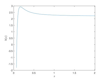
   Figure 1: Example graph of $h(z)$ when $1-\gamma>\frac{\mu-r}{\sigma^{2}}$.

   Based on above results, $h(z)>0$ leads to $z>v_{1}$ for some positive real number $v_{1}$. Therefore, $\nu^{*}\xi_{T}<f_{\lambda}(Y)$ is equivalent to $\xi_{T}>v_{1}$, and Formula (3.7) becomes

   $$C^{*}_{t}=\mathbb{E}\left[Z_{t}\left(\left(\frac{\nu^{*}\xi_{t}Z_{t}}{\gamma}\right)^{\frac{1}{\gamma-1}}+g(\xi_{t}Z_{t})\right)\mathds{1}_{\{\xi_{t}Z_{t}>v_{1}\}}\bigg{|}\mathcal{F}_{t}\right]=n(\xi_{t},t),$$ (3.8)

   where

   $$\!\!\!n(z,t)= \mathbb{E}\left[Z_{t}\left(\left(\frac{\nu^{*}zZ_{t}}{\gamma}\right)^{\frac{1}{\gamma-1}}+g(zZ_{t})\right)\mathds{1}_{\{zZ_{t}>v_{1}\}}\right]$$

   $$= \left(\frac{\gamma}{\nu^{*}}\right)^{\frac{1}{1-\gamma}}z^{\frac{1}{\gamma-1}}\mathbb{E}\left[Z_{t}^{\frac{\gamma}{\gamma-1}}\mathds{1}_{\{Z_{t}>\frac{v_{1}}{z}\}}\right]$$

   $$+a\eta z^{b}\mathbb{E}\left[Z_{t}^{b+1}\mathds{1}_{\{\frac{v_{1}}{z}<Z_{t}<\frac{c}{z}\}}\right]\!-\!k\eta e^{rT}\mathbb{E}\left[Z_{t}\mathds{1}_{\{\frac{v_{1}}{z}<Z_{t}<\frac{c}{z}\}}\right].$$

   Using Proposition 2 yields

   $$n(z,t)= D_{1}z^{\frac{1}{\gamma-1}}H_{t}\left(\frac{v_{1}}{z},\frac{\gamma}{\gamma-1}\right)+D_{2}z^{b}\left[H_{t}\left(\frac{v_{1}}{z},b+1\right)-H_{t}\left(\frac{c}{z},b+1\right)\right]$$ (3.9)

   $$-k\eta e^{rt}\left[H_{t}\left(\frac{v_{1}}{z},1\right)-H_{t}\left(\frac{c}{z},1\right)\right],$$

   where $D_{1}=\left(\frac{\gamma}{\nu^{*}}\right)^{\frac{1}{1-\gamma}}e^{\frac{\gamma}{\gamma-1}(T-t)\left(\frac{\theta^{2}}{2\gamma-2}-r\right)}$, $D_{2}=a\eta e^{-\frac{\mu+r}{2}(b+1)(T-t)}$.

   To derive the optimal strategy $\{m_{t}^{*},0\leqslant t\leqslant T\}$ from the optimal $C_{t}^{*}$ for Problem (3.5), using Itô’s formula we obtain

   $$\mathrm{d}C_{t}^{*}=\frac{\partial n}{\partial z}(\xi_{t},t)\mathrm{d}\xi_{t}+\frac{\partial n}{\partial t}(\xi_{t},t)\mathrm{d}t+\frac{\theta^{2}}{2}\frac{\partial^{2}n}{\partial z^{2}}(\xi_{t},t)\xi_{t}^{2}\mathrm{d}t.$$

   Comparing the last equation with Eq.(3.1), we have

   $$m^{*}_{t}=-\frac{\theta\xi_{t}}{\sigma C_{t}^{*}}\frac{\partial n}{\partial z}(\xi_{t},t)=-\frac{\theta}{\sigma C^{*}_{t}}M(\xi_{t},t),$$ (3.10)

   where $M(z,t)=z\frac{\partial n}{\partial z}(z,t)$ and has the following expression in this case:

   $$M(z,t)= \frac{D_{1}}{\gamma-1}z^{\frac{1}{\gamma-1}}H_{t}\left(\frac{v_{1}}{z},\frac{\gamma}{\gamma-1}\right)+bD_{2}z^{b}\left[H_{t}\left(\frac{v_{1}}{z},b+1\right)-H_{t}\left(\frac{c}{z},b+1\right)\right]$$ (3.11)

   $$+\frac{D_{1}z^{\frac{1}{\gamma-1}}}{\theta\sqrt{T-t}}G_{t}\left(\frac{v_{1}}{z},\frac{\gamma}{\gamma-1}\right)+\frac{D_{2}z^{b}}{\theta\sqrt{T-t}}\left[G_{t}\left(\frac{v_{1}}{z},b+1\right)-G_{t}\left(\frac{c}{z},b+1\right)\right]$$

   $$-\frac{k\eta e^{rt}}{\theta\sqrt{T-t}}\left[G_{t}\left(\frac{v_{1}}{z},1\right)-G_{t}\left(\frac{c}{z},1\right)\right].$$

2. If $1-\gamma<\frac{\mu-r}{\sigma^{2}}$. In this case, we can verify the following properties of $h$ (see Figures 3 & 3 for examples):

   $$h(0+)=+\infty,~{}h^{\prime}(0+)=-\infty,~{}h(+\infty)>0,\text{ and }h^{\prime}(z)>0\text{ for }z>z_{2},$$

   where $z_{2}$ is a positive real number.

   Based on above properties of $h$, the condition $\nu^{*}\xi_{T}<f_{\lambda}(Y)$ finally leads to two more cases:

   1. $\xi_{T}>0$;

   2. $\xi_{T}\in(0,v_{2})\cup(v_{3},+\infty)$, where $v_{2}$ and $v_{3}$ are some real numbers satisfying $0<v_{2}<v_{3}<c$.

   

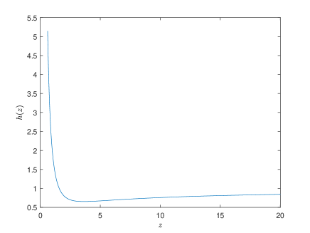
   Figure 2: Example graph of $h$ for Case 2-(i).

   

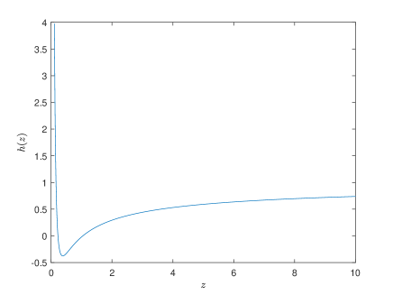
   Figure 3: Example graph of $h$ for Case 2-(ii).

   Using Proposition 2, we can find out the expression of $C_{t}^{*}=n(\xi_{t},t)$ and $m^{*}_{t}=-\frac{\theta}{\sigma C^{*}_{t}}M(\xi_{t},t)$.

   For Case 2-(i), $n$ and $M$ can be obtained by letting $v_{1}\rightarrow 0^{+}$ in (3.9) and (3.11), and we have

   $$n(z,t)=D_{1}z^{\frac{1}{\gamma-1}}+D_{2}z^{b}\left[1-H_{t}\left(\frac{c}{z},b+1\right)\right]-k\eta e^{rt}\left[1-H_{t}\left(\frac{c}{z},1\right)\right],$$ (3.12)

   $$M(z,t)= \frac{D_{1}}{\gamma-1}z^{\frac{1}{\gamma-1}}+bD_{2}z^{b}\left[1-H_{t}\left(\frac{c}{z},b+1\right)\right]-\frac{D_{2}z^{b}}{\theta\sqrt{T-t}}G_{t}\left(\frac{c}{z},b+1\right)$$ (3.13)

   $$+\frac{k\eta e^{rt}}{\theta\sqrt{T-t}}G_{t}\left(\frac{c}{z},1\right).$$

   For Case 2-(ii), we have

   $$n(z,t)= D_{1}z^{\frac{1}{\gamma-1}}\left[H_{t}\left(\frac{v_{3}}{z},\frac{\gamma}{\gamma-1}\right)-H_{t}\left(\frac{v_{2}}{z},\frac{\gamma}{\gamma-1}\right)+1\right]$$

   $$+D_{2}z^{b}\left[H_{t}\left(\frac{v_{3}}{z},b+1\right)-H_{t}\left(\frac{c}{z},b+1\right)-H_{t}\left(\frac{v_{2}}{z},b+1\right)+1\right]$$

   $$-k\eta e^{rt}\left[H_{t}\left(\frac{v_{3}}{z},1\right)-H_{t}\left(\frac{c}{z},1\right)-H_{t}\left(\frac{v_{2}}{z},1\right)+1\right],$$

   $$M(z,t)= \frac{D_{1}z^{\frac{1}{\gamma-1}}}{\gamma-1}\left[H_{t}\left(\frac{v_{3}}{z},\frac{\gamma}{\gamma-1}\right)-H_{t}\left(\frac{v_{2}}{z},\frac{\gamma}{\gamma-1}\right)+1\right]$$ (3.14)

   $$+bD_{2}z^{b}\left[H_{t}\left(\frac{v_{3}}{z},b+1\right)-H_{t}\left(\frac{c}{z},b+1\right)-H_{t}\left(\frac{v_{2}}{z},b+1\right)+1\right]$$

   $$+\frac{D_{1}z^{\frac{1}{\gamma-1}}}{\theta\sqrt{T-t}}\left[G_{t}\left(\frac{v_{3}}{z},\frac{\gamma}{\gamma-1}\right)-G_{t}\left(\frac{v_{2}}{z},\frac{\gamma}{\gamma-1}\right)\right]$$

   $$+\frac{D_{2}z^{b}}{\theta\sqrt{T-t}}\left[G_{t}\left(\frac{v_{3}}{z},b+1\right)-G_{t}\left(\frac{c}{z},b+1\right)-G_{t}\left(\frac{v_{2}}{z},b+1\right)\right]$$

   $$-\frac{k\eta e^{rt}}{\theta\sqrt{T-t}}\left[G_{t}\left(\frac{v_{3}}{z},1\right)-G_{t}\left(\frac{c}{z},1\right)-G_{t}\left(\frac{v_{2}}{z},1\right)\right].$$

3. If $1-\gamma=\frac{\mu-r}{\sigma^{2}}$, then $h(z)=(d_{1}-a)z^{b}+ke^{rT}$, and $\nu^{*}\xi_{T}<f_{\lambda}(Y)$ finally leads to $\xi_{T}>v_{4}$ for some constant $v_{4}\in[0,c)$. The case reduces to Case 1.

Summarizing the above derivations, we have the following theorem for the optimal risk multiplier.

Theorem 2.

The optimal risk multiplier is given by

$$m^{*}_{t}=-\frac{\theta}{\sigma C^{*}_{t}}M(\xi_{t},t),$$

where $C^{*}_{t}=n(\xi_{t},t)$ and

1. when $1-\gamma\geqslant\frac{\mu-r}{\sigma^{2}}$, $n(z,t)$ and $M(z,t)$ are given by (3.9) and (3.11), respectively.

2. when $1-\gamma<\frac{\mu-r}{\sigma^{2}}$, $n(z,t)$ and $M(z,t)$ are given by (3.12)–(3.14), repsectively.

Recall that we have established an optimal solution $C_{T}^{*}$ for Problem (3.5) for every $\lambda\geqslant 0$. By utilizing numerical methods, we can determine the zero point $\lambda^{*}$ of the function $f(\cdot)$. After obtaining $\lambda^{*}$, we determine the corresponding category in which it falls and employ the related expressions for $n$ and $M$ to derive the optimal multiplier process $\{m_{t}^{*},0\leqslant t\leqslant T\}$. The numerical results will be presented in the following section.

4 Numerical results

In this section, we present the numerical results for Problem (2.3). For the market parameter settings, we consider $\mu=0.1435$ and $\sigma=0.17$, which are estimated using the average return of the S&P 500 Index from 2012 to 2021. Additionally, we set $r=0.0088$ based on the US 10-year Treasury Yield during the same period. Regarding the model settings, we choose $T=5$ years, $k=0.9$, $\eta=0.7$, and $\gamma=0.5$.

We employ the Monte Carlo method to simulate both the market price, denoted as $\{S_{t},0\leqslant t\leqslant T\}$, and the cushion, denoted as $\{C_{t},0\leqslant t\leqslant T\}$, under various PPI strategies. These strategies involve fixed values of the risk multiplier $m$ selected from the set $\{2,3,4,5,6,8,10\}$, in addition to the optimal risk multiplier determined in our research. Furthermore, we consider the specific choice of $m=\frac{\mu-r}{(1-\gamma)\sigma^{2}}=9.32$, which corresponds to the optimal strategy for a CRRA utility function $u(x)=x^{\gamma}$. Our simulations are conducted with the assumption of 260 trading days per year. In alignment with the methodology described in Zieling et al., (2014), we introduce a borrowing constraint by implementing the condition $m_{t}C_{t}\leqslant 2V_{t}$ in our simulations. This condition ensures that whenever $m_{t}C_{t}$ exceeds $2V_{t}$, we restrict $m_{t}$ to the level of $\frac{2V_{t}}{C_{t}}$. To maintain the stability of the simulation process, particularly when the term $C_{t}^{*}$ in the denominator of (3.10) approaches zero, we constrain the values of $m^{*}_{t}$ to fall within the interval $[0,20]$.

4.1 Comparisons with CPPI strategies

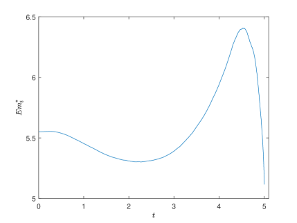
Figure 4: Mean of $m^{*}_{t}$.

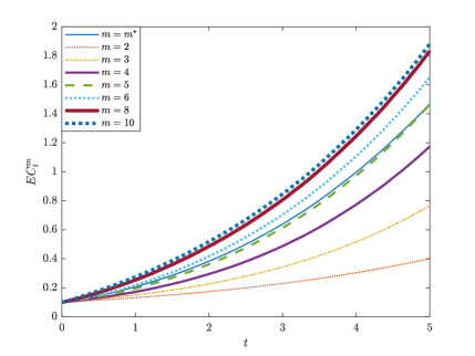
Figure 5: Mean of $C^{m}_{t}$ under different $m$.

In Figure 5, the mean of $m^{*}_{t}$ exhibits a distinct hump-shaped pattern. Similar to the outcomes observed under utility functions characterized by loss aversion, investors tend to increase their allocation to the risky asset as they approach the maturity date. This strategic shift is aimed at mitigating potential losses and capitalizing on the prospects of higher returns through a sort of investment “gambling”. Specifically, in the baseline model where the risky asset performs well, this shift towards gambling behavior is relatively gradual. Consequently, it results in the optimal $m^{*}_{t}$ falling within the range of $[5,6.5]$. Notably, the optimal $m^{*}_{t}$ remains below the value of $m=\frac{\mu-r}{(1-\gamma)\sigma^{2}}=9.32$. This discrepancy can be attributed to the influence of loss aversion, which encourages a more cautious approach with lower leverage.

In Figure 5, we conduct a comparison of the mean values of $C^{m}_{t}$ across different $m$ settings. The results reveal a positive correlation between the mean of $C^{m}_{t}$ and the parameter $m$. Furthermore, the optimal excess value exhibits a gradual increase over time. This trend can be attributed to the performance of the risky asset, where higher leverage results in greater returns. However, it is important to note that employing higher leverage also introduces higher downside risk. As a result, the optimal case based on the mean criterion may not necessarily align with achieving the highest utility when considering the Omega ratio.

To conduct a comprehensive comparison of performance under different $m$ values, we calculate several performance indicators for each $m$ as follows:

• $E_{1}$: the expected utility of the numerator in the extended Omega ratio (2.3)

• $E_{2}$: the expected utility of the denominator in the extended Omega ratio (2.3)

• $OR$: the extended Omega ratio $\frac{E1}{E2}$

• $E[C_{T}]$: the expectation of the terminal cushion $C_{T}$

• $P_{liq}$: the probability of liquidation (i.e., $C_{T}<0$)

• $P$: the probability that the terminal cushion $C_{T}$ is less than the benchmark $Y$

Furthermore, for each constant $m$, we calculate the winning rate of $m^{*}$ against the constant $m$, which represents the probability that the terminal cushion $C_{T}^{m}$ under the constant strategy $m$ is smaller than $C_{T}^{m^{*}}$. We denote this winning rate as $WR$.

Table 1: Performance results for $m^{*}$ and constant multiplier strategies

	$E_{1}$	$E_{2}$	$OR$	$P_{liq}$	$P$	$WR$	$E[C_{T}]$
$m^{*}$	0.505	0.123	4.11	0.0	63.3%	-	1.470
2	0.014	0.568	0.02	0.0	66.8%	75.7%	0.402
3	0.132	0.335	0.39	0.0	21.0%	75.4%	0.768
4	0.367	0.230	1.60	0.0	40.8%	70.4%	1.175
5	0.519	0.204	2.54	0.0	50.0%	44.6%	1.468
6	0.605	0.203	2.98	0.0	53.6%	29.2%	1.655
8	0.677	0.226	3.00	0.0	54.5%	31.4%	1.836
10	0.692	0.261	2.65	0.0	52.6%	45.6%	1.884
$\frac{\mu-r}{(1-\gamma)\sigma^{2}}$	0.691	0.249	2.78	0.0	53.4%	39.5%	1.877

The findings highlight several notable trends. First, there is a positive correlation between the expected utility of the numerator ($E_{1}$) in the Omega ratio and the parameter $m$, indicating that higher leverage results in increased returns. Conversely, the expected utility of the denominator ($E_{2}$) in the Omega ratio exhibits an interesting pattern. Initially, it decreases as $m$ is enlarged, but then it begins to increase. The initial decrease in $E_{2}$ can be attributed to the reduction of insufficient leverage, which hinders effective tracking of the benchmark. The subsequent increase in $E_{2}$ is a consequence of excessive leverage, which can lead to higher downside risk.

Remarkably, the expected utility of the denominator in the Omega ratio is the smallest under the optimal value of $m^{*}$, and the probability of the terminal excess value $C_{T}$ falling below the benchmark $Y$ is the second highest in this case. These seemingly contradictory results can be attributed to the strategy designed to maximize the Omega ratio. Initially, investors select a moderate value for $m^{*}$. As the maturity date approaches, the performance of the risky asset and the high excess value of the fund incentive investors to take on some level of risk, positively impacting the tracking of the upward benchmark. However, there is a higher likelihood of falling below the benchmark in the latter stages due to the larger leverage. Nevertheless, these later strategies can be effectively and timely adjusted, reducing the associated gap and resulting in relatively small negative utility. Furthermore, several other observations can be made. The Omega ratio is maximized at the optimal value of $m^{*}$, and the minimum guarantee is fully protected in all cases. Although the ideal winning rate is not achieved, the strategy $m^{*}$ maximizes the Omega ratio by closely tracking the benchmarks and minimizing the gaps.

Figure 6: Theoretical optimal Omega ratio.

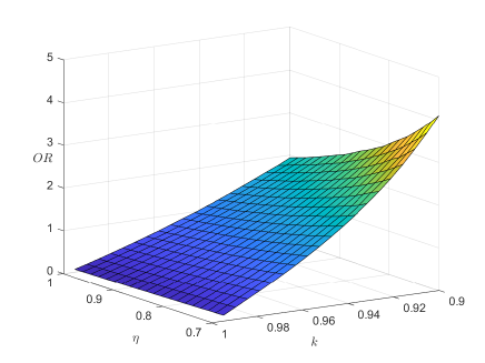
Figure 7: Realized Omega ratio.

Additionally, we have generated a plot illustrating the Omega ratio as it varies with different values of $\eta$ and $k$. It is important to note that in Proposition 1, a requirement is set that $1-k<\mathbb{E}[\xi_{T}Y]$, which is equivalent to $0.2\eta+k>1$ given the current parameter settings. Therefore, we have selected the intervals $k\in[0.9,1]$ and $\eta\in[0.7,1]$ as the target range where this inequality automatically holds. As our simulations are conducted in a discrete setting, the realized Omega ratio $OR$ (Figure 7) may not perfectly align with the theoretical optimal Omega ratio $\lambda$ (Figure 7). Nevertheless, both figures exhibit a similar overall trend. It is evident that the Omega ratio exhibits a negative correlation with both $k$ and $\eta$. A higher value of $k$ increases the challenge of safeguarding the minimum guarantee and limits investment flexibility. Likewise, a larger value of $\eta$ heightens the difficulty of tracking the upward benchmark and reduces the capacity for returns.

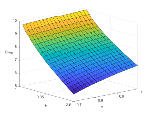
Figure 8: $\mathbb{E}[m_{0}]$.

Furthermore, we depict the relationship between $\mathbb{E}[m_{0}]$ and the parameters $(\eta,k)$ in Figure 8. Notably, as $k$ increases, the excess value $C$ decreases in response. This reduction in excess value results in reduced investment flexibility, necessitating an increase in the expected risky proportion $\mathbb{E}[m_{0}]$ to counter the adverse effects. Similarly, when $\eta$ takes on larger values, it becomes more challenging to effectively track the upward benchmark. Consequently, the expected risky proportion $\mathbb{E}[m_{0}]$ must also be elevated to achieve better tracking performance. In summary, the risky multiplier is positively correlated with both $k$ and $\eta$.

4.2 Sensitivity test

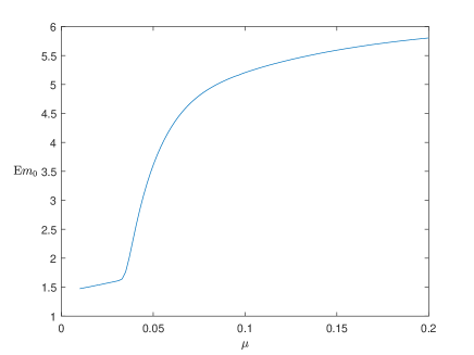
(a) Relationshiop between $\mathbb{E}m_{0}$ and $\mu$.

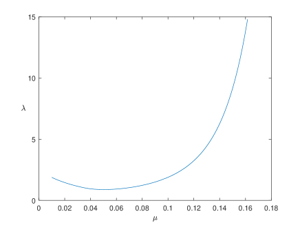
(b) Relationshiop between $\lambda$ and $\mu$.

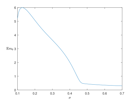
(c) Relationshiop between $\mathbb{E}m_{0}$ and $\sigma$.

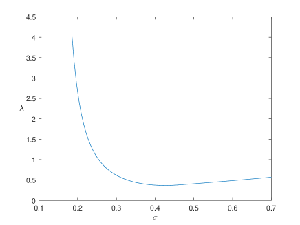
(d) Relationshiop between $\lambda$ and $\sigma$.

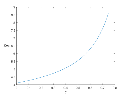
(e) Relationshiop between $\mathbb{E}m_{0}$ and $\gamma$.

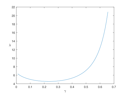
(f) Relationshiop between $\lambda$ and $\gamma$.

Figure 9: Sensitivity analysis.

In this subsection, we present the relationships between $(OR,\mathbb{E}[m_{0}])$ and the market parameters $(\mu,\sigma,\gamma)$ in Figure 9. As Figure 7 and Figure 7 indicate that the theoretical Omega ratio $\lambda$ and the realized Omega ratio $OR$ exhibit a similar trend, we use $\lambda$ instead of $OR$ in the following figures because the latter requires much more calculation than the former. Figures 9-(a) and 9-(b) illustrate the impacts of $\mu$ on $\mathbb{E}[m_{0}]$ and $\lambda$. The influence of $\mu$ can be outlined in three key aspects. First, a higher expected return for the risky asset results in a more frequent occurrence of an upward benchmark. Second, this upward benchmark that needs to be tracked increases accordingly. Last, the actual return on investments in the risky asset also experiences an increase. These combined effects lead to a larger proportion of the portfolio allocated to risky investments as $\mu$ increases. Furthermore, when $\mu$ increases, the Omega ratio initially decreases and then increases. In the initial stage, the increase in $\mu$ transforms the benchmark from a downside protection level to an upward tracking benchmark. This transition elevates the challenge of achieving positive returns, thereby reducing the Omega ratio. In the latter stage, the performance of risky investment returns becomes exceptionally robust. Under such circumstances, not only is the benchmark tracked effectively, but also substantial excess returns are generated. As a result, the Omega ratio increases with the increase of $\mu$.

In Figures 9-(c) and 9-(d), we investigate the effects of $\sigma$ on $\mathbb{E}m_{0}$ and $\lambda$. The findings indicate that both $\mathbb{E}m_{0}$ and $\lambda$ exhibit negative correlations with $\sigma$. When $\sigma$ increases, it introduces heightened volatility in both upward and downward directions. In particular, the increased downward volatility has a substantial adverse impact on the Omega ratio, leading investors to reduce their allocation to risky assets.

Figures 9-(e) and 9-(f) examine the effects of $\gamma$ on $\mathbb{E}m_{0}$ and $\lambda$. The outcomes reveal that both $\mathbb{E}m_{0}$ and $\lambda$ exhibit positive correlations with $\gamma$. As $\gamma$ increases, investors exhibit a reduced level of risk aversion. In such a scenario, investors favor allocating a higher proportion to risky assets. Additionally, the weakening of loss aversion, as indicated by the increasing $\gamma$, contributes to an overall elevation in the Omega ratio.

5 Conclusion

In this paper, we study the optimal risk multiplier within the VPPI strategy, which enables investors to adjust their risk exposure based on market conditions. Our objective is to maximize the extended Omega ratio while incorporating a binary stochastic benchmark. To address the non-concave nature of this optimization problem, we employ the stochastic version of the concavification technique, which enables us to derive semi-analytical solutions for the optimal risk multiplier. The value functions are divided into three categories, depending on the relationship between the fixed risk multiplier introduced in the previous work by Zieling et al., (2014) and the value 1.

The findings of this study reveal that the optimal risk multiplier exhibits a hump-shaped pattern and tends to be lower compared to fixed multipliers. This suggests that investors adopt a cautious approach influenced by loss aversion. Our results highlight that, due to the influence of loss aversion, investors tend to favor lower leverage at the beginning and strategically pursue larger positive returns as the maturity date approaches. Interestingly, although the over-performance probability and winning rate may not reach ideal levels, the VPPI strategy excels in maximizing the Omega ratio through close benchmark tracking and reduced negative gaps. Moreover, the impact of performance parameters, such as the guarantee ratio and capturing ratio, has a multifaceted effect on both investment and benchmark performance.

Acknowledgements

The authors acknowledge support from the National Natural Science Foundation of China (Grant Nos. 12371477, 11901574, 12271290, 11871036), the MOE Project of Key Research Institute of Humanities and Social Sciences (22JJD910003), and the National Social Science Fund of China (20AZD075). The authors thank the members of the group of Mathematical Finance and Actuarial Science at the Department of Mathematical Sciences, Tsinghua University for their feedback and useful conversations.

Appendix A Proof of main results

Proof of Theorem 1.

Define

$$\underline{X}_{\lambda}(z,y)=\min\mathcal{X}_{\lambda}(z,y)=\left\{\begin{aligned} &~{}~{}0,~{}&&z\geqslant f_{\lambda}(y),\\ &\left(\frac{z}{\gamma}\right)^{\frac{1}{\gamma-1}}+y,~{}&&z<f_{\lambda}(y),\end{aligned}\right.$$

and $g(\nu)=\mathbb{E}\left[\xi_{T}\underline{X}_{\lambda}\left(\nu\xi_{T},Y\right)\right]$ for $\nu>0$. As $\xi_{T}$ is log-normal distributed, the expectation is always well-defined, and one can verify $g(0+)=+\infty$, $g(+\infty)=0$. Therefore, Proposition 1 and Theorem 3 in Liang et al., (2021) ensure the existence of optimal solution to Problem (3.5) and the finiteness of Problem (3.5) for all $k\in(0,1)$. Moreover, the random set $\mathcal{X}_{\lambda}\left(\nu\xi_{T},Y\right)$ is not single-valued if and only if $\nu\xi_{T}=f_{\lambda}(Y)$, which is equivalent to

$$d\left[\eta\left(a\xi_{T}^{b}-ke^{rT}\right)\mathds{1}_{\{\xi_{T}<c\}}\right]^{\gamma-1}=\nu\xi_{T}.$$

As the probability that the above equation holds is $0$, Theorem 3 in Liang et al., (2021) ensures the uniqueness of the optimal solution and the continuity of $g$. Therefore, there exists $\nu^{*}>0$ such that $g(\nu^{*})=1-k$, and again Theorem 3 ensures that $\underline{X}_{\lambda}\left(\nu^{*}\xi_{T},Y\right)$ is the optimal solution to Problem (3.5). ∎

Proof of Proposition 1.

First, we prove that $f$ is finite. As $\xi_{T}$ is log-normal distributed, Proposition 1 in Liang et al., (2021) ensures that the problem $\sup\limits_{C_{T}\in\mathcal{C}}~{}\mathbb{E}\left[U(C_{T}-Y)\mathds{1}_{\{C_{T}>Y\}}\right]$ has a finite optimal value $v_{1}$. Therefore, we have $-\lambda\mathbb{E}\left[U(Y)\right]\leqslant f(\lambda)\leqslant v_{1}.$

Second, we prove that $f$ is continuous. For $0\leqslant\lambda_{1}<\lambda_{2}$, we have

$$f(\lambda_{1}) =\sup_{C_{T}\in\mathcal{C}}~{}\left\{\mathbb{E}\left[U(C_{T}-Y)\mathds{1}_{\{C_{T}>Y\}}\right]-\lambda_{1}\mathbb{E}\left[U(Y-C_{T})\mathds{1}_{\{C_{T}\leqslant Y\}}\right]\right\}$$

$$\leqslant f(\lambda_{2})+(\lambda_{2}-\lambda_{1})\sup_{C_{T}\in\mathcal{C}}\mathbb{E}\left[U(Y-C_{T})\mathds{1}_{\{C_{T}\leqslant Y\}}\right]$$

$$\leqslant f(\lambda_{2})+(\lambda_{2}-\lambda_{1})\mathbb{E}\left[U(Y)\right].$$

According to the definition of $f$, we know $f(\lambda_{2})\leqslant f(\lambda_{1})$. Therefore, we have

$$|f(\lambda_{2})-f(\lambda_{1})|\leqslant(\lambda_{2}-\lambda_{1})\mathbb{E}\left[U(Y)\right],$$

which indicates that $f$ is continuous.

Third, we prove $v_{2}\triangleq\inf\limits_{C_{T}\in\mathcal{C}}\mathbb{E}\left[U(Y-C_{T})\mathds{1}_{\{C_{T}\leqslant Y\}}\right]>0.$ Indeed, Theorem 3 in Liang et al., (2021) ensures that the problem $\sup\limits_{C_{T}\in\mathcal{C}}\mathbb{E}\left[-U(Y-C_{T})\mathds{1}_{\{C_{T}\leqslant Y\}}\right]$ admits an optimal solution $C^{*}$. Noting that $\mathbb{E}\left[\xi_{T}C^{*}_{T}\right]\leqslant 1-k<\mathbb{E}\left[\xi_{T}Y\right]$, it is impossible that $C^{*}_{T}\geqslant Y$ holds almost everywhere. Therefore, $v_{2}=\mathbb{E}\left[U(Y-C^{*}_{T})\mathds{1}_{\{C^{*}_{T}\leqslant Y\}}\right]>0.$

Using the results above, we obtain $f(\lambda)\leqslant v_{1}-\lambda v_{2}$. The inequality indicates that $f(\lambda)<0$ for sufficiently large $\lambda$. Recall that $f$ is continuous and $f(0)=v_{1}\geqslant 0$, the intermediate value theorem guarantees a zero point $\lambda^{*}$ for $f$.

For this zero point $\lambda^{*}$, we know

$$0=f(\lambda^{*})=\sup_{C_{T}\in\mathcal{C}}~{}\left\{\mathbb{E}\left[U(C_{T}-Y)\mathds{1}_{\{C_{T}>Y\}}\right]-\lambda^{*}\mathbb{E}\left[U(Y-C_{T})\mathds{1}_{\{C_{T}\leqslant Y\}}\right]\right\}.$$

This indicates that $\mathbb{E}\left[U(C_{T}-Y)\mathds{1}_{\{C_{T}>Y\}}\right]-\lambda^{*}\mathbb{E}\left[U(Y-C_{T})\mathds{1}_{\{C_{T}\leqslant Y\}}\right]\leqslant 0$ holds for every $C_{T}\in\mathcal{C}$. Noting that $\mathbb{E}\left[\xi_{T}Y\right]>1-k\geqslant\mathbb{E}\left[\xi_{T}C_{T}\right]$, we have $\mathbb{E}\left[U(Y-C_{T})\mathds{1}_{\{C_{T}\leqslant Y\}}\right]>0$. Therefore, the following inequality holds:

$$\frac{\mathbb{E}\left[U(C_{T}-Y)\mathds{1}_{\{C_{T}>Y\}}\right]}{\mathbb{E}\left[U(Y-C_{T})\mathds{1}_{\{C_{T}\leqslant Y\}}\right]}\leqslant\lambda^{*}.$$

As $C_{T}^{*}$ is an optimal solution to the optimization problem $f(\lambda^{*})$, we have

$$0=f(\lambda^{*})=\mathbb{E}\left[U(C_{T}^{*}-Y)\mathds{1}_{\{C_{T}^{*}>Y\}}\right]-\lambda^{*}\mathbb{E}\left[U(Y-C_{T}^{*})\mathds{1}_{\{C_{T}^{*}\leqslant Y\}}\right],$$

and hence

$$\frac{\mathbb{E}\left[U(C_{T}^{*}-Y)\mathds{1}_{\{C_{T}^{*}>Y\}}\right]}{\mathbb{E}\left[U(Y-C_{T}^{*})\mathds{1}_{\{C_{T}^{*}\leqslant Y\}}\right]}=\lambda^{*}.$$

This result shows that $\lambda^{*}$ is the optimal value of Problem (3.2) and $C_{T}^{*}$ is an optimal solution. ∎

References

- Ameur and Prigent, (2014) Ameur, H. B. and Prigent, J.-L. (2014). Portfolio insurance: Gap risk under conditional multiples. European Journal of Operational Research, 236(1):238–253.
- Annaert et al., (2009) Annaert, J., Van Osselaer, S., and Verstraete, B. (2009). Performance evaluation of portfolio insurance strategies using stochastic dominance criteria. Journal of Banking and Finance, 33(2):272–280.
- Balder et al., (2009) Balder, S., Brandl, M., and Mahayni, A. (2009). Effectiveness of CPPI strategies under discrete-time trading. Journal of Economic Dynamics and Control, 33(1):204–220.
- Bernard et al., (2019) Bernard, C., Vanduffel, S., and Ye, J. (2019). Optimal strategies under Omega ratio. European Journal of Operational Research, 275(2):755–767.
- Bertrand and Prigent, (2001) Bertrand, P. and Prigent, J.-L. (2001). Portfolio insurance strategies: OBPI versus CPPI. Finance, 26(1):5–32.
- Bertrand and Prigent, (2011) Bertrand, P. and Prigent, J.-L. (2011). Omega performance measure and portfolio insurance. Journal of Banking and Finance, 35(7):1811–1823.
- Bertrand and Prigent, (2016) Bertrand, P. and Prigent, J.-L. (2016). Extreme Events in Finance: A Handbook of Extreme Value Theory and Its Applications. Wiley Online Library.
- Biedova and Steblovskaya, (2020) Biedova, O. and Steblovskaya, V. (2020). Multiplier optimization for constant proportion portfolio insurance (CPPI) strategy. International Journal of Theoretical and Applied Finance, 23(02):2050011.
- Black and Jones, (1987) Black, F. and Jones, R. (1987). Simplifying portfolio insurance. Journal of Portfolio Management, 14(1):48.
- Branger et al., (2010) Branger, N., Mahayni, A., and Schneider, J. C. (2010). On the optimal design of insurance contracts with guarantees. Insurance: Mathematics and Economics, 46(3):485–492.
- Carpenter, (2000) Carpenter, J. N. (2000). Does option compensation increase managerial risk appetite? The Journal of Finance, 55(5):2311–2331.
- Cesari and Cremonini, (2003) Cesari, R. and Cremonini, D. (2003). Benchmarking, portfolio insurance and technical analysis: a Monte Carlo comparison of dynamic strategies of asset allocation. Journal of Economic Dynamics and Control, 27(6):987–1011.
- Chen et al., (2008) Chen, J. S., Chang, C. L., Hou, J. L., and Lin, Y. T. (2008). Dynamic proportion portfolio insurance using genetic programming with principal component analysis. Expert Systems with Applications, 35(1-2):273–278.
- Cox and Huang, (1989) Cox, J. C. and Huang, C. F. (1989). Optimal consumption and portfolio policies when asset prices follow a diffusion process. Journal of Economic Theory, 49(1):33–83.
- De Giorgi and Post, (2011) De Giorgi, E. G. and Post, T. (2011). Loss aversion with a state-dependent reference point. Management Science, 57(6):1094–1110.
- Dehghanpour and Esfahanipour, (2017) Dehghanpour, S. and Esfahanipour, A. (2017). A robust genetic programming model for a dynamic portfolio insurance strategy. In 2017 IEEE International Conference on INnovations in Intelligent SysTems and Applications (INISTA), pages 201–206. IEEE.
- Dichtl and Drobetz, (2011) Dichtl, H. and Drobetz, W. (2011). Portfolio insurance and prospect theory investors: Popularity and optimal design of capital protected financial products. Journal of Banking and Finance, 35(7):1683–1697.
- Dinkelbach, (1967) Dinkelbach, W. (1967). On nonlinear fractional programming. Management Science, 13(7):492–498.
- Guastaroba et al., (2016) Guastaroba, G., Mansini, R., Ogryczak, W., and Speranza, M. G. (2016). Linear programming models based on omega ratio for the enhanced index tracking problem. European Journal of Operational Research, 251(3):938–956.
- Hambardzumyan and Korn, (2019) Hambardzumyan, H. and Korn, R. (2019). Dynamic hybrid products with guarantees-an optimal portfolio framework. Insurance: Mathematics and Economics, 84:54–66.
- Happersberger et al., (2020) Happersberger, D., Lohre, H., and Nolte, I. (2020). Estimating portfolio risk for tail risk protection strategies. European Financial Management, 26(4):1107–1146.
- He and Kou, (2018) He, X. D. and Kou, S. (2018). Profit sharing in hedge funds. Mathematical Finance, 28(1):50–81.
- He and Strub, (2022) He, X. D. and Strub, M. S. (2022). How endogenization of the reference point affects loss aversion: a study of portfolio selection. Operations Research, 70(6):3035–3053.
- Herold et al., (2007) Herold, U., Maurer, R., Stamos, M., and Vo, H. T. (2007). Total return strategies for multi-asset portfolios. Journal of Portfolio Management, 33(2):60.
- Kane et al., (2009) Kane, S. J., Bartholomew-Biggs, M. C., Cross, M., and Dewar, M. (2009). Optimizing omega. Journal of Global Optimization, 45(1):153–167.
- Kapsos et al., (2014) Kapsos, M., Christofides, N., and Rustem, B. (2014). Worst-case robust Omega ratio. European Journal of Operational Research, 234(2):499–507.
- Karatzas et al., (1991) Karatzas, I., Lehoczky, J. P., Shreve, S. E., and Xu, G. L. (1991). Martingale and duality methods for utility maximization in an incomplete market. SIAM Journal on Control and optimization, 29(3):702–730.
- Karatzas et al., (1998) Karatzas, I., Shreve, S. E., Karatzas, I., and Shreve, S. E. (1998). Methods of Mathematical Finance, volume 39. Springer.
- Keating and Shadwick, (2002) Keating, C. and Shadwick, W. F. (2002). A universal performance measure. Journal of Performance Measurement, 6(3):59–84.
- Lee et al., (2008) Lee, H. I., Chiang, M. H., and Hsu, H. (2008). A new choice of dynamic asset management: the variable proportion portfolio insurance. Applied Economics, 40(16):2135–2146.
- Leland, (1980) Leland, H. E. (1980). Who should buy portfolio insurance? The Journal of Finance, 35(2):581–594.
- Liang et al., (2021) Liang, Z., Liu, Y., and Zhang, L. (2021). A framework of state-dependent utility optimization with general benchmarks. arXiv preprint arXiv:2101.06675.
- Lin et al., (2019) Lin, H., Saunders, D., and Weng, C. (2019). Portfolio optimization with performance ratios. International Journal of Theoretical and Applied Finance, 22(05):1950022.
- Schied, (2014) Schied, A. (2014). Model-free cppi. Journal of Economic Dynamics and Control, 40:84–94.
- Sprenger, (2015) Sprenger, C. (2015). An endowment effect for risk: Experimental tests of stochastic reference points. Journal of Political Economy, 123(6):1456–1499.
- Weng, (2013) Weng, C. (2013). Constant proportion portfolio insurance under a regime switching exponential Lévy process. Insurance: Mathematics and Economics, 52(3):508–521.
- Zhang et al., (2015) Zhang, T., Zhou, H., Li, L., and Gu, F. (2015). Optimal rebalance rules for the constant proportion portfolio insurance strategy-evidence from China. Economic Systems, 39(3):413–422.
- Zieling et al., (2014) Zieling, D., Mahayni, A., and Balder, S. (2014). Performance evaluation of optimized portfolio insurance strategies. Journal of Banking and Finance, 43:212–225.