OrthCaps: An Orthogonal CapsNet with Sparse Attention Routing and Pruning

Abstract

Redundancy is a persistent challenge in Capsule Networks (CapsNet), leading to high computational costs and parameter counts. Although previous works have introduced pruning after the initial capsule layer, dynamic routing’s fully connected nature and non-orthogonal weight matrices reintroduce redundancy in deeper layers. Besides, dynamic routing requires iterating to converge, further increasing computational demands. In this paper, we propose an Orthogonal Capsule Network (OrthCaps) to reduce redundancy, improve routing performance and decrease parameter counts. Firstly, an efficient pruned capsule layer is introduced to discard redundant capsules. Secondly, dynamic routing is replaced with orthogonal sparse attention routing, eliminating the need for iterations and fully connected structures. Lastly, weight matrices during routing are orthogonalized to sustain low capsule similarity, which is the first approach to introduce orthogonality into CapsNet as far as we know. Our experiments on baseline datasets affirm the efficiency and robustness of OrthCaps in classification tasks, in which ablation studies validate the criticality of each component. Remarkably, OrthCaps-Shallow outperforms other Capsule Network benchmarks on four datasets, utilizing only 110k parameters – a mere 1.25% of a standard Capsule Network’s total. To the best of our knowledge, it achieves the smallest parameter count among existing Capsule Networks. Similarly, OrthCaps-Deep demonstrates competitive performance across four datasets, utilizing only 1.2% of the parameters required by its counterparts. The code is available at https://github.com/ornamentt/Orthogonal-Capsnet.

1 Introduction

While convolutional Neural Networks (CNNs) excel in computer vision tasks, certain challenges remain, which include information loss in pooling layers, low robustness, and poor spatial feature correlation [28, 7]. To address these limitations, Capsule Network (CapsNet) was proposed, using capsule vectors instead of traditional neurons. In CapsNet, each capsule vector’s length represents the presence probability of specific entities in the input image, and its direction encodes the captured features [28]. This setup allows the capsule vectors to capture features related to corresponding entities. CapsNet’s architecture includes a primary capsule extraction layer, a digit capsule layer, dynamic routing, and class-conditioned reconstruction. As a key component of CapsNet, dynamic routing aligns lower-level capsules with higher-level ones, which is described in Fig. 1. First, lower-level capsules $U_{l}$ (in matrix form) predict poses $\hat{U}_{l}$ for higher-level capsules $V_{l+1}$ via weight matrix $W$. Then, the routing process iteratively clusters to adjust the coupling coefficients $c_{ij}$ of each lower-level capsule $u_{l,i}$ to all higher-level capsules, with more crucial capsules receiving larger $c_{ij}$. The algorithm is in Sec. 9.

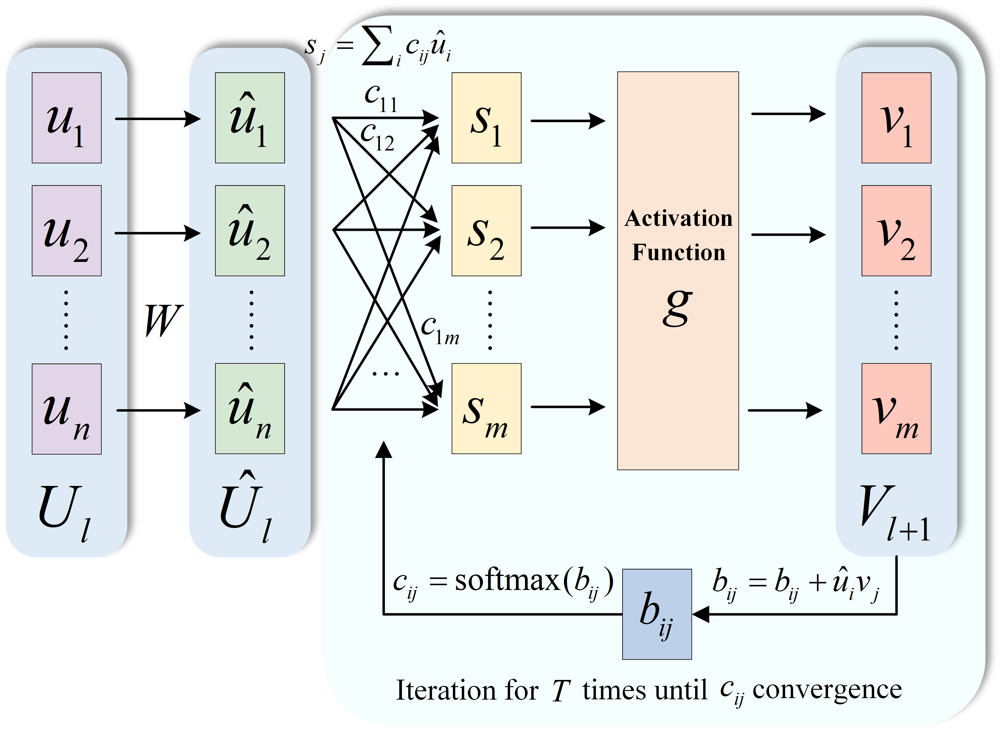
Figure 1: Dynamic routing mechanism. $u_{i},v_{j}$ are the lower-level capsule, and higher-level capsule, respectively. $W$ is the weight matrix to produce the pose prediction $\hat{u}_{i}$ of $u_{i}$ for next level. $b_{ij}$ is a temporary variable to calculate the coupling coefficient $c_{ij}$.

Recent studies have mentioned that Capsnet contains redundant capsules [1, 29, 26]. As evidence, Fig. 2 shows 48.2% of primary capsule pairs exhibit cosine similarities above 0.65, indicating significant redundancy.

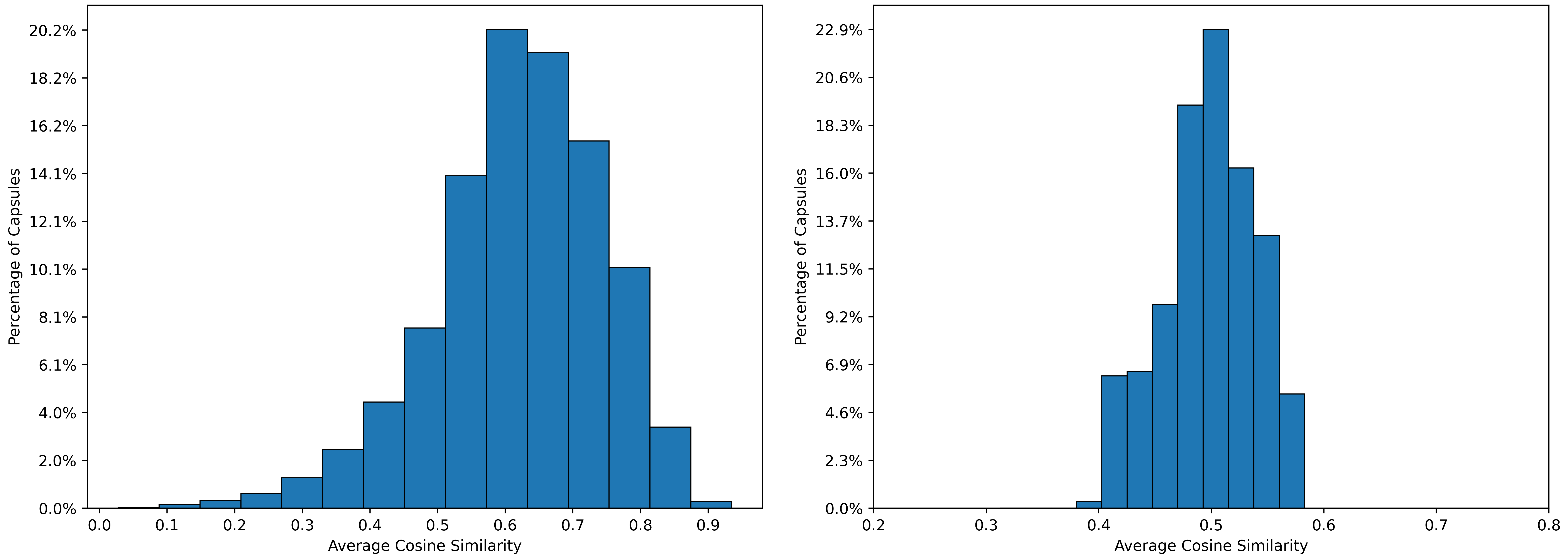
Figure 2: Left: In the primary capsule layer of CapsNet, 48.2% of capsule pairs have cosine similarities greater than 0.65, indicating significant redundancy among capsules. Right: After introducing the Pruned Layer, capsule similarities effectively decrease. (Detailed in Section 3.2)

Although certain studies have implemented pruning techniques at the primary capsule layer [27], deeper layers still show considerable over-similar issues, as demonstrated in Fig. 6. We attribute this persistent redundancy in deeper layers to dynamic routing. On the one hand, since $v_{l+1,j}=g(\sum_{i}c_{ij}\hat{u}_{l,i})$, each higher-level capsule is essentially a weighted sum of lower-level capsules, indicating a fully connected structure between lower and higher layers in CapsNet [13]. This full connection leads to a potential transmission of redundant information. On the other hand, considering $\hat{U}_{l}=WU_{l}$, we can express higher-level capsules as $V_{l+1}=g[(C*W)U_{l}]$. Non-orthogonal matrices $C*W$ in routing may increase the reduced capsule similarity after pruning, which not only impairs routing performance but also reintroduces redundancies in subsequent layers. Additionally, dynamic routing requires multiple iterations to repeatedly update $c_{ij}$ until convergence, further straining computational resources.

Inspired by the successful use of orthogonality in CNNs[36] and Transformer[9] to reduce filter overlaps, we introduce the Orthogonal Capsule Network(OrthCaps). OrthCaps has two versions: the lightweight OrthCaps-Shallow (OrthCaps-S) and the OrthCaps-Deep (OrthCaps-D). OrthCaps addresses the above problems of the fully connected structure of dynamic routing, increasing similarity in deep layers, and the need for iteration, detailed as follows:

Firstly, we introduce a pruned capsule layer after the primary capsule layer, which eliminates redundant capsules and retains only essential and representative ones. Here, capsules are firstly ordered by importance, then their cosine similarity is calculated to identify redundant capsules. Beginning with the least important, the process consistently prunes capsules that exceed the similarity threshold, proceeding through the entire set of capsules.

Secondly, to solve the iteration issue, dynamic routing is replaced with attention routing, which is a straightforward routing mechanism. To solve the fully connected problem, we leverage sparsemax-based attention to produce an attention map, which selectively amplifies relevant feature groups corresponding to specific entities while downplaying irrelevant ones. For OrthCaps-S, a simplified attention-routing is adopted, optimizing parameter counts.

Thirdly, to address the issue of increased capsule similarity in deeper layers, we introduce orthogonality into capsule networks. By applying Householder orthogonal decomposition, we enforce orthogonality in the weight matrices during attention routing. Orthogonal weight matrices sustain low inter-capsule correlation, which encourages fewer capsules to represent more features during backpropagation, thereby enhancing accuracy while effectively reducing the number of parameters.

Contributions. To summarize our work, we make the following contributions:

1) To our knowledge, this approach addresses the issue of deep redundancy in Capsule Networks for the first time. A novel pruned strategy is implemented to alleviate capsule redundancy and an orthogonal sparse attention routing mechanism is proposed to replace dynamic routing.

2) It is the first time orthogonality has been introduced into Capsule Networks as far as we know. This simple, penalty-free orthogonalization method is also adaptable to other neural networks.

3) Two OrthCaps versions are created: OrthCaps-S and OrthCaps-D. OrthCaps-S sets a new benchmark in accuracy with just 1.25% of CapsNet’s parameters on datasets of MNIST, SVHN, smallNORB, and CIFAR10. OrthCaps-D excels on CIFAR10, CIFAR100 and FashionMNIST while keeping parameters minimal.

2 Related Work

Capsule Networks. Dynamic routing was first introduced by Sabour et al.[28]. Though numerous studies have used attention strategies to improve dynamic routing, the issue of the fully connected structure and reintroduction of redundancy remains unaddressed [8, 21, 19]. Choi et al. incorporated attention into the capsule routing via a non-iterative feed-forward operation [2]. Tsai et al. introduced a parallel iterative routing, which did not address the complexity of iterative requirements [33]. Furthermore, many works focused on pruning but did not mention new redundancies introduced by dynamic routing [13, 29, 27]. Jeong et al. established a ladder structure, using a pruning algorithm based on encoding [13]. Sharifi et al. created a pruning layer based on Taylor Decomposition [29]. Renzulli et al. used LOBSTER to create a sparse tree [27]. Different from existing works, we incorporate pruning, orthogonality and sparsity to effectively reduce redundancy.

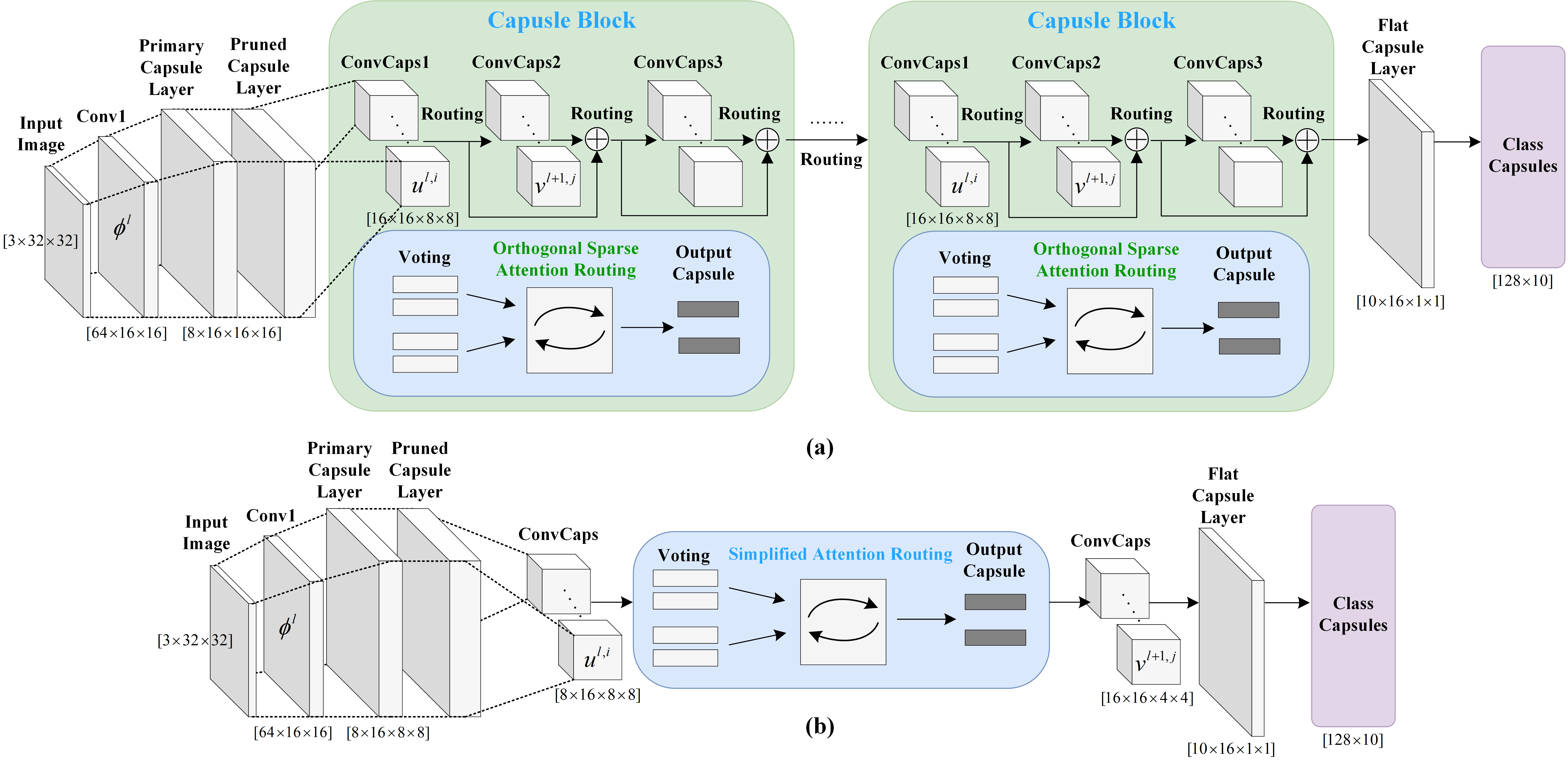
Figure 3: (a): In CIFAR10 classification task, the OrthCaps-D model comprises 7 capsule blocks, each with 3 capsule layers, interconnected via shortcut connections and orthogonal sparse attention routing. (b): The OrthCaps-S model contains two capsule layers coping with CIFAR10 and does not use any capsule layer with MNIST. These layers are linked through simplified attention routing.

Orthogonality. Various methods were proposed to introduce orthogonality into neural networks, which can be categorized into hard and soft orthogonality. Hard orthogonality maintains matrix orthogonality throughout training by either optimizing over the Stiefel manifold [17, 10], or parameterizing a subset of orthogonal matrices [32, 31, 35]. These methods incur computational overhead and result in vanishing or exploding gradients. Soft orthogonality, on the other hand, employs a regularization term in the loss function to encourage orthogonality among column vectors of weight matrix without strict enforcement [36, 24, 11]. Yet, strong regularization overshadows the primary task loss, while weak regularization fails to encourage orthogonality. We leverage Householder orthogonal decomposition [34, 18] to achieve strict matrix orthogonality, minimizing computational complexity and obviating the need for additional regularization terms.

3 Methodology

3.1 Overall Architecture

We introduce OrthCaps, offering both shallow (OrthCaps-S) and deep (OrthCaps-D) architectures to minimize parameter counts while exploring the potential for deep multi-layer capsule networks.

As illustrated in Fig. 3a, OrthCaps-D comprises five key components: a convolutional layer, a primary capsule layer, a pruned capsule layer, seven capsule blocks and a flat capsule layer. Given input images $x\in\mathbb{R}^{(B,3,W,H)}$, initial features $\Phi^{0}\in\mathbb{R}^{(B,C,W^{0},H^{0})}$ are extracted through a convolutional layer. The primary capsule layer generates initial capsules $u^{1}\in\mathbb{R}^{(B,n,d,W^{1},H^{1})}$ with a kernel size of 3 and stride of 2. $B,n,d,C$ represent the batch size, number of capsules, capsule dimensions and channels, respectively. A pruned capsule layer is then placed to remove redundant capsules. OrthCaps-D has seven capsule blocks, each containing three depthwise convolutional capsule layers(ConvCaps Layers) linked by shortcut connections to prevent vanishing gradient. Within each block, lower-level capsules $u^{l}$ are routed to the next layer $v^{l+1}$ via orthogonal sparse attention routing. Blocks are also connected through routing, allowing for stacking to construct deeper capsule networks. The flatcaps layer is employed to map capsules into classification categories for final classification tasks.

OrthCaps-S, as illustrated in Fig. 3b, replaces the complete attention routing with a simplified version and has a single block within capsule layers. The number of layers can be adjusted as needed. Convolutional capsules in the primary layer utilize a 9x9 kernel with a stride of 1, and other layers are consistent with OrthCaps-D.

3.2 Pruned Capsule Layer

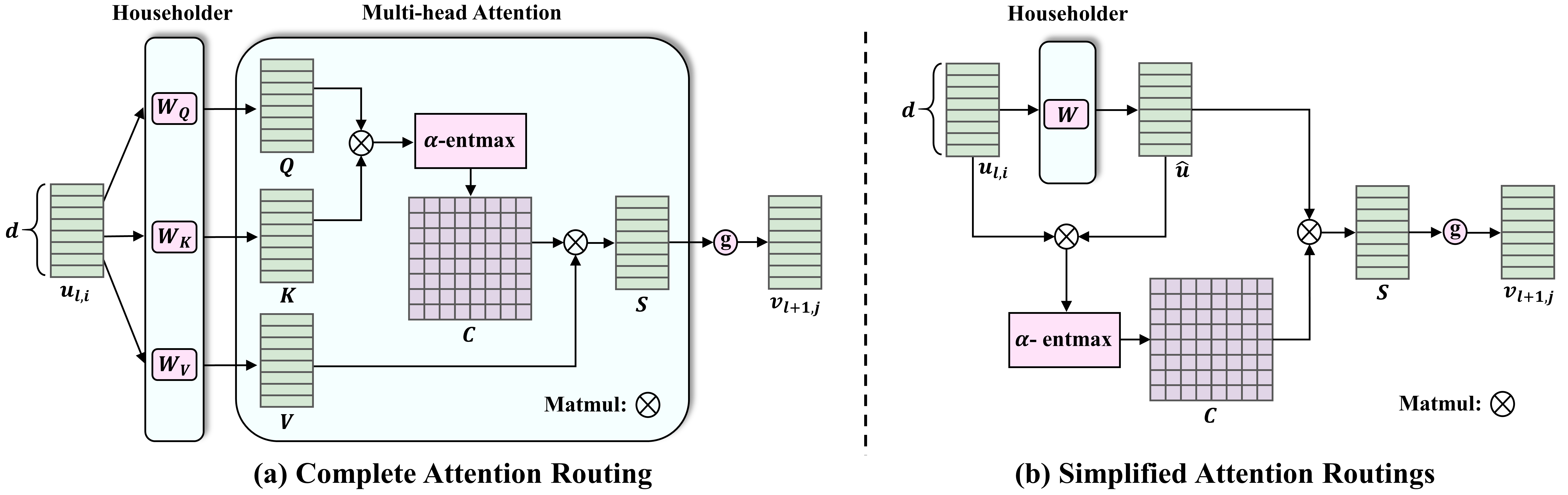
Figure 4: Orthogonal self-attention routing.

The generation of capsules starts with the primary capsule layer. At this initial stage, it is crucial to generate low-correlated capsules, which ensures efficient feature representation and reduces feature overlap during subsequent layers. Therefore, we introduce an efficient capsule pruning algorithm 1, including the following parts:

Redundancy Definition. Redundancy occurs when two capsules capture identical or similar features. Given that the direction of each capsule vector encodes specific features, capsules with closer directions(or angles) indicate that they capture similar features and entities. Thus, we employ the cosine similarity of capsule angles to measure redundancy.

Capsule Importance Ordering. For redundant capsule pairs, random pruning may result in losing capsules vital for accurate classification. To ensure that the less crucial capsule is pruned first when the similarity between a pair is high, capsules are sorted in an order based on $\|u_{flat}\|_{2}$. We employ $L_{2}$-norm as it calculates the length of capsule vectors, indicating the existence probability of encoded entities, which shows the activeness of capsules [13].

Pruning. After ordering, a mask matrix $M\in\mathbb{R}^{(1,n,1)}$ is initialized to all-ones. Starting with the least active capsule, the process computes the cosine similarity between less active capsule $u_{\text{ordered},i}$ with more active capsule $u_{\text{ordered},j}$. When the similarity exceeds the threshold $\theta$, the corresponding column in the mask for $u_{\text{ordered},i}$ is set to 0, indicating that less active capsule is pruned. In this way, only the active capsules are retained all along. The final step is applying $M$ to $u_{\text{ordered}}$, producing pruned capsules $u_{\text{pruned}}$. $n^{\prime}$ is the number of remaining capsules after pruning.

Algorithm 1 Efficient Capsule Pruning

1:Capsules $u\in\mathbb{R}^{(B,n,d,W,H)}$, threshold $\theta$

2:$u_{\text{pruned}}\in\mathbb{R}^{(B,n,d,W,H)}$

3:Reshape $u$ $\rightarrow$ $u_{\text{flat}}\in\mathbb{R}^{(B,n,(d\times W\times H))}$

4:Compute $L_{2}$-norm: $\|u_{\text{flat}}\|_{2}$

5:Order capsules by $L_{2}$-norm: $u_{\text{flat}}\rightarrow u_{\text{ordered}}$

6:Initialize $M$: all-ones matrix

7:for $i<j$ do

8:   $t_{ij}=\text{cosine\_similarity}(u_{\text{ordered},i},u_{\text{ordered},j})$

9:   $m_{i}=0$ where $t_{ij}>\theta$

10:Prune using $M$: $u_{\text{pruned}}=u_{\text{ordered}}\odot M$

11:Reshape $u_{\text{pruned}}$ to $u_{\text{pruned}}\in\mathbb{R}^{(B,n^{\prime},d,W,H)}$

12:return $u_{\text{pruned}}$

Notably, we compute the cosine similarity matrix $T$ by broadcasting, which avoids explicit for-loop iteration and reduces computational complexity. The 5D capsule tensor of $u_{l}$ with dimensions $d$ and number $n$, $[B,n,d,W,H]$, is reshaped to $[B,n,d\times W\times H]$ to suit for broadcasting.

3.3 Routing Algorithm

We introduce the orthogonal sparse attention routing to replace dynamic routing. This approach eliminates the need for iteration and leverages sparsity to reduce redundant feature transmission.

Let $u_{l,i}$ and $v_{l+1,j}$ represent capsules at layer $l$ and $l+1$ respectively, each with dimension $d$. We employ three weight matrices $W_{Q}$, $W_{K}$, $W_{V}\in\mathbb{R}^{d\times d}$ to derive queries $Q$, keys $K$, and values $V$ from $u_{l,i}$, $Q=W_{Q}\times u_{l,i},K=W_{K}\times u_{l,i},V=W_{V}\times u_{l,i}$. Specifically, $W_{Q}$, $W_{K}$, and $W_{V}$ are designed as orthogonal matrices, enabling them to project $u_{l,i}$ into a $d$-dimensional orthogonal subspace.

As shown in Fig. 4a, attention routing aims to produce coupling coefficient $c_{ij}$, which serves as the weight during routing from lower-level to higher-level capsules. The coupling coefficient matrix $C$ is derived from the attention map, generated through the dot product of $Q$ and $K$, $C=\alpha\text{-Entmax}(QK^{T}/\sqrt{d})$. Here, we replace the softmax of the original attention mechanism with $\alpha$-Entmax in Eq. 1, enhancing the sparsity of the attention map. $\alpha$-Entmax adaptively sets small $c_{ij}$ to zero, thereby encouraging routing to prioritize more important capsules while minimizing irrelevant information transfer.

$$\alpha\text{-Entmax}(x)_{i}=\max\left(\frac{x_{i}-\tau}{\alpha},0\right)^{\frac{1}{\alpha-1}}\vspace*{-5pt}$$ (1)

$\tau$ is a self-adaption threshold and $\alpha$ is a hyperparameter controlling the sparsity of the attention map.

The vote $s_{l+1,j}$ is computed as the product of $V$ and $C$. In LABEL:S_{i and LABEL:j}, higher-level capsule $v_{l+1,j}$ is generated by $s_{l+1,j}$ from a multi-head self-attention mechanism with 16 heads, using the nonlinear activation function $g$.

$$v_{l+1,j}=g(s_{l+1,j})=g(\alpha\text{-Entmax}(QK^{T}/\sqrt{d})\times V)\vspace*{-5pt}$$ (2)

For simplified attention-routing in Fig. 4b, we condense prediction matrices $W$ from three to one and replace $K,Q,V$ with $u_{l,i}$ [6]. The $\hat{u}_{l,i}$ is the prediction for $v_{l+1,j}$. The attention map $C$ is obtained using $\alpha$-entmax with the dot product to produce the vote $s_{l+1,j}$ $=\hat{u}_{l,i}\times C=\hat{u}_{l,i}\times(\alpha\text{-Entmax}(\hat{u}_{l,i}u_{l,i}^{T}/\sqrt{d}))$. $s_{l+1,j}$ is processed through $g$ to produce $v_{l+1,j}$. Notably, standard convolutions are supplanted by depthwise convolutions to minimize parameter count. Without any iteration, attention routing reduces computational complexity.

3.4 Orthogonalization

In Sec. 3.2, we reduce redundancy by pruning highly similar capsules. To preserve pruning effect in subsequent layers, it’s vital to maintain low similarity among capsules all along. Here, capsules with diverse angles span a broader multi-dimensional feature subspace, enabling the network to capture a wider array of features with fewer capsules, which boosts accuracy and reduces parameter count.

We utilize orthogonalization to achieve this. An orthogonal matrix, signifying a rotation or reflection transformation, keeps vector lengths and inter-vector angles constant during multiplication with a vector set. Considering that cosine similarity quantifies angles between vectors, applying an orthogonal matrix $W$ to a vector set retains the mutual cosine similarity among all vector pairs in the set. Let $\{v_{l+1,j}\mid j=1,2,\ldots,m\}$ be a set of capsule vectors at layer $l+1$, we derive Lemma 1:

Lemma 1: For any $i,j\in\{1,2,\ldots,m\}$, if $W$ is orthogonal, the cosine similarity between $v_{l+1,i}$ and $v_{l+1,j}$ remains unchanged after multiplication by $W$.

Sec. 3.4.1 discusses the selection of targets for orthogonalization, while Sec. 3.4.2 details the method.

3.4.1 Orthogonalization of Weight Matrices

The goal of orthogonalization is to maintain low similarity among higher-level capsules. Following Sec. 3.3, we represent higher-level capsules into matrix multiplication:

$$V_{l+1}=g(S_{l})=g(CV)=g[(C\times W_{V})U_{l}]\vspace*{-5pt}$$ (3)

As the activation function $g$ in CapsNet preserves the capsule vector’s direction [28], in line with Lemma 1, ensuring orthogonality of $C$ and $W_{V}$ can maintain low similarity. However, orthogonalizing $C$ directly is hard, so we delve deeper into its calculation process in Eq. 4:

Since $d$ is a constant, it requires no additional analysis. The impact of $U_{l}{U_{l}}^{T}$ on orthogonalizing $C$ is mitigated by pruning, which removes capsules with short lengths and high cosine similarity. Consequently, the remaining capsules were updated to approximate unit length and low correlation, akin to a standard orthonormal basis. Thus, $U_{l}{U_{l}}^{T}$ gradually becomes more orthogonal as the network trains, minimizing its impact on the orthogonality of $C$. Although $\alpha\text{-Entmax}$, a nonlinear function, may not preserve the orthogonality of inputs, it renders $C$ sparse. This sparsity directs lower-level capsules effectively toward their respective higher-level targets, which reduces interference during routing, thus encouraging a relatively low similarity among higher-level capsules.

Our above analysis indicates that orthogonalizing $W_{Q},W_{K}$, and $W_{V}$ is essential for maintaining low cosine similarity among higher-level capsules. While $C$ is not fully orthogonalized, our experiments demonstrate considerable improvements in both accuracy and parameter efficiency.

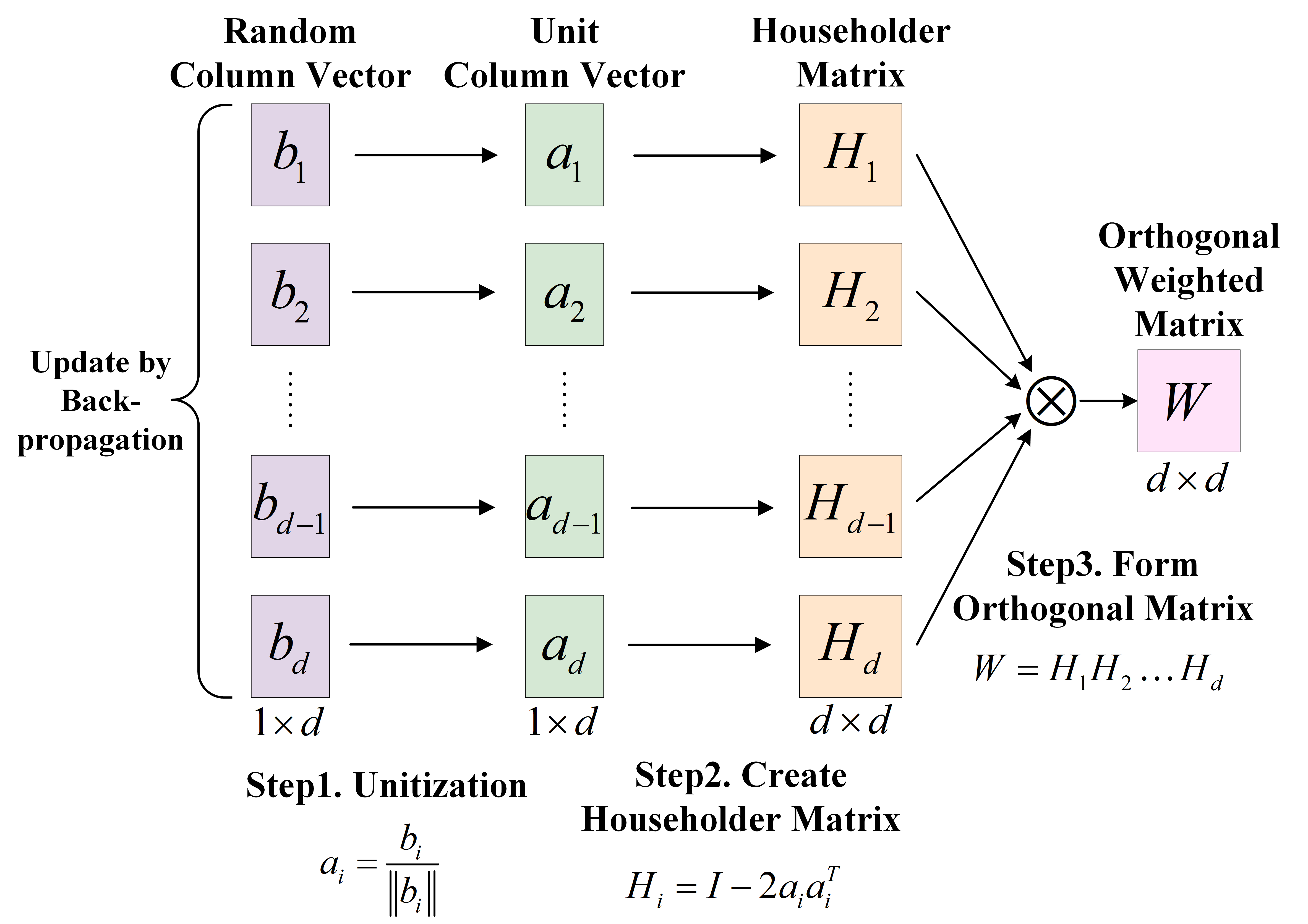
Figure 5: The computing process of HouseHolder method.

3.4.2 Householder Orthogonalization

Let $W$ be the weight matrix requiring orthogonalization. As shown in Fig. 5, the Householder orthogonal decomposition theorem is employed to formulate an endogenously optimizable orthogonal matrix. The essence of this approach is in the following algebraic lemma [34]:

Lemma 2: Any orthogonal $n\times n$ matrix is the product of at most $n$ orthogonal Householder transformations.

Based on Lemma 2, an orthogonal matrix $W\in\mathbb{R}^{d\times d}$ can be formulated in Eq. 5:

$$W=H_{0}H_{1}\dots H_{d-1}\vspace*{-5pt}$$ (5)

Each $H_{i}$ represents a Householder transformation, defined as $H_{i}=I-2a_{i}a_{i}^{T}$, where $a_{i}$ is a unit column vector. We utilize a set of randomly generated column vectors $\{b_{i}|i=0,\dots,d-1\}$ instead of $a_{i}$ to construct $H_{i}$ as detailed in Eq. 6. During training, $b_{i}$ is optimized through gradient backpropagation. $W$ inherently preserves its orthogonality during training.

$$W=\prod_{i=0}^{d-1}\left(I-\frac{2b_{i}b_{i}^{T}}{{\|b_{i}\|}^{2}}\right)\vspace*{-5pt}$$ (6)

Lemma 3: $W_{Q}$, $W_{K}$, and $W_{V}$ constructed using Equation Eq. 6 are Orthogonal.

Following Eq. 6, $W_{Q}$, $W_{K}$, and $W_{V}$ could easily be orthogonalized, where the proof is provided in supplement material Sec. 8.2. Householder orthogonalization enables computationally efficient transformation of arbitrary coefficient matrices into orthogonal matrices without any additional penalty terms in the loss function.

4 Experiments

4.1 Experimental Setup

Table 1: (a): OrthCaps-S ranks as the top or second best across five datasets, standing out as being resource-efficient with only 105.5K parameters and 673.1M FLOPS. (b): OrthCaps-D shows competitive performance with fewer parameters and less computational cost.

Shallow Networks	Param$\downarrow$	FLOPS[M]$\downarrow$	MNIST	SVHN	smallNORB	CIFAR10
OrthCaps-S	105.5K	673.1	99.68	96.26	98.30	86.84
Efficient-Caps	162.4K	631.1	99.58	93.12	97.46	81.51
CapsNet	8388K	803.8	99.52	91.36	95.42	68.72
Matrix-CapsNet with EM routing	450K	949.6	99.56	87.42	95.56	81.39
AR CapsNet	9.1M	2562.7	99.46	85.98	96.47	85.39
DA-CapsNet	7M*	-	99.53*	94.82*	98.26*	85.47*
AA-CapsNet	6.6M*	-	99.34*	91.23*	89.72*	79.41*
Baseline CNN	4.6M	1326.9	99.22	91.28	87.11	72.20

(a) (a)

Deep Networks	Param $\downarrow$	FLOPS[M]$\downarrow$	CIFAR10	CIFAR100	MNIST	FashionMNIST
OrthCaps-D	574K	3345	90.56	70.56	99.59	94.60
AR-CapsNet(7 ensembled)	6.3M	16657.5	88.94	56.53	99.49	91.73
CapsNet(7 ensembled)	5.8M*	5137.4*	89.4*	-	-	-
Inverted Dot-Product	1.4M	5340.9	84.98	57.32	99.35	92.85
RS-CapsNet	5.0M*	-	89.81*	64.14*	-	93.51*
DeepCaps	13.5M	2687	91.01	69.72	99.46	92.52
ResNet-18	11.7M	5578.8	95.10	77.60	99.29	93.32
VGG-16	147.3M	15143.1	93.57	73.10	99.21	92.21

(b) (b)

Implementation Details and Datasets

OrthCaps was developed using PyTorch 1.12.1, running on Python 3.9, and the training process was accelerated using four GTX-3090 GPUs. We adopted the margin loss as defined in [28]. Observing minimal performance benefits in our experiments, we decided to exclude the reconstruction loss. Our model utilized the AdamW optimizer with a cosine annealing learning rate scheduler and a 5-cycle linear warm-up. We set learning rate at 5e-3, weight decay at 5e-4, and batchsize at 512. We conducted experiments on SVHN [20], smallNORB [16], CIFAR10, and MNIST [15] for OrthCaps-S. OrthCaps-D was evaluated on CIFAR10, CIFAR100 [14], Fashion-MNIST [37], and MNIST. We resized SmallNORB from $96\times 96$ to $64\times 64$ and cropped it to $48\times 48$ like [28]. All other datasets retained original sizes. For data augmentation, we adopted the methods outlined in [7]. For reproducibility, we detailed hyperparameters and setups in supplement material Sec. 7.1.

Comparison Baselines

OrthCaps was benchmarked against a range of baseline models to evaluate its performance. For OrthCaps-S, we compared it with Efficient-Caps[19], CapsNet[28], Matrix-CapsNet with EM routing[7], AR-CapsNet[2], AA-CapsNet[23], DA-CapsNet[12] and standard 7-layer CNN. For OrthCaps-D, we used baselines such as CapsNet (7 ensembles), AR-CapsNet (7 ensembles), RS-CapsNet[38], Inverted Dot-Product[33], DeepCaps[25], ResNet-18[5], and VGG-16[30]. All comparative results were derived from running official codes with our hyperparameters.

4.2 Classification Performance Comparison

Tab. 1(b) illustrates the classification performance of OrthCaps-S and OrthCaps-D, with model sizes denoted by Param and computational demands represented as FLOPS[M]. All models utilize a backbone of 4 convolutional layers and undergo training for 300 epochs. The Param and FLOPS[M] of each table are tested on MNIST and CIFAR10, respectively. An asterisk (*) signifies that no official code is available, so we refer to the model performance stated in the original papers.

As shown in Tab. 1(b)a, OrthCaps-S achieves superior efficiency with merely 105.5K parameters, outperforming CNN, CapsNet, and many variants. For instance, Efficient-Caps, a state-of-the-art model on efficiency, has about 50% more parameters. Despite its compact design, OrthCaps-S either outperforms or matches the performance of other capsule networks across all four datasets. On the SVHN and CIFAR10, OrthCaps-S achieves accuracies of 96.26% and 87.92%, respectively, surpassing CapsNet which has 80 times more parameters. With a computational demand of 673.1M FLOPS, it’s worth noting that the slight increase in FLOPS compared to Efficient-Caps is due to the additional computations from the pruned capsule layer and orthogonal transformations. Given the substantial decrease in parameter count and the enhanced accuracy, this FLOPS trade-off is warranted.

For OrthCaps-D, as illustrated in Tab. 1(b)b, it exhibits competitive performance with fewer parameters and less computational cost on complex datasets. Although convolution-based networks such as ResNet-18 and VGG-16 perform well on CIFAR10 and CIFAR100, OrthCaps-D offers competitive performance using just 1.41% and 0.11% of their parameters as well as 56% and 20.8% of their FLOPS, respectively. The efficiency of OrthCaps becomes evident when compared with DeepCaps. While DeepCaps achieves a 91.01% accuracy on CIFAR10, its significant parameter count of 13.42M highlights a compromise. It’s noteworthy that both OrthCaps variants maintain high performance with fewer parameters.

4.3 Ablation Study

4.3.1 Orthogonal Attention Routing

Through a cross-comparison of frames-per-second (FPS) and accuracy on two datasets with different complexity, as shown in Tab. 2, we compare attention routing with dynamic routing[28] and sparse softmax with standard softmax, respectively. Additionally, $\alpha$ is settled to 1.5 in our experiments according to [22].

Table 2: Comparison of Orthogonal sparse attention routing and dynamic routing algorithms. FPS is tested under MNIST dataset.

Variants	FPS$\uparrow$	MNIST	CIFAR10
Attention routing & $\alpha$-entmax & orthogonality	1639	99.68	86.92
Attention routing & softmax	1785	99.62	83.44
Dynamic routing & $\alpha$-entmax & orthogonality	1232	99.51	70.01
Dynamic routing & softmax	1339	99.49	68.72

Attention routing consistently outperforms dynamic routing in both classification accuracy and processing speed, achieving a 25.8% speed enhancement on average. Even with a faster softmax, dynamic routing only reaches 1339 FPS, indicating its inherent computational inefficiencies. Although $\alpha$-entmax’s complexity and the additional computational demands from orthogonality slightly reduce processing speed compared to softmax, this trade-off is justified by a substantial increase in accuracy and robustness (detailed in Sec. 4.5). Overall, our attention routing combined with $\alpha$-entmax and orthogonality balances performance and computational efficiency.

4.3.2 Pruned Capsule Layer

Fig. 2 illustrates that by integrating the pruned layer, the average capsule similarity decreases due to redundant capsule elimination. Consequently, as the capsule count reduces, the dimensions of the associated prediction matrix diminish, thereby lowering the parameter count. This is proved in Tab. 3, where the pruned OrthCaps-S reduces parameters from 127K to 105K without sacrificing performance. In fact, accuracy improves from 99.53% to 99.68% and from 85.32% to 87.92% on MNIST and CIFAR10, respectively. Similarly, applying pruning to CapsNet results in higher accuracy with reduced parameters (7492K from 8388K). This shows our pruning method’s efficacy in streamlining the model and enhancing performance.

Table 3: CapsNets are compared with and without the pruning layer, with the similarity threshold set to 0.7. Param[K] is tested on MNIST.

Variant	Param[K]$\downarrow$	MNIST	CIFAR10
OrthCaps-S with pruning	105	99.68	87.92
OrthCaps-S	157	99.53	85.32
Capsnet with pruning	7492	99.51	71.08
Capsnet	8388	99.42	68.72

Fig. 6 illustrates the necessity of incorporating pruning with orthogonality. Capsule similarity is gauged with cosine similarity to measure the redundancy as mentioned above. As the network goes deeper, the dashed line (indicating pruning without orthogonality) shifts rightward, suggesting an increase in capsule similarity. This shift proves that non-orthogonal weight matrices reintroduce redundancy. However, the solid line (indicating pruning with orthogonality) shows consistently low capsule similarity. Even at 28 layers deep, the similarity remains low, affirming the efficacy of orthogonality in preserving capsule directions to maintain low inter-capsule correlations. The black dash-dot line denotes similarity without orthogonality and pruning, exhibiting the highest redundancy, further evaluating the effectiveness of our method.

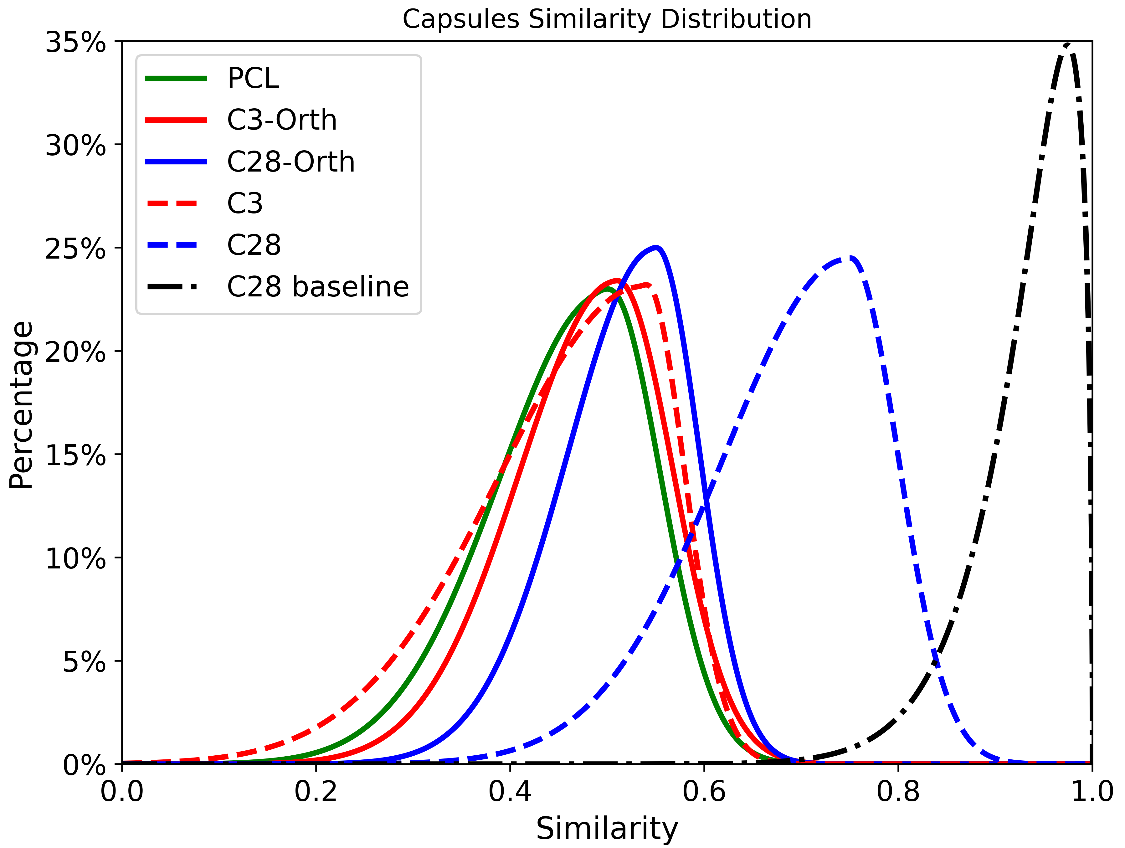
Figure 6: Redundancy comparison between different pruning strategies. (The more to the left, the better.) The x-axis shows capsule similarity; the y-axis indicates capsule count percentage. PCL, C3, and C28 mark the primary, third, and twenty-eighth capsule layers. Solid lines (C3-Orth, C28-Orth) and dashed lines represent pruning with and without orthogonality, respectively; the dash-dot line indicates the absence of both pruning and orthogonality. Tests are on OrthCaps-D with CIFAR10 dataset.

4.4 Similarity Threshold

To find the optimal similarity threshold $\theta$, we evaluated the classification accuracy on three datasets and capsule number after pruning (N) for thresholds ranging from 0.3 to 1.0. At $\theta=1.0$, the pruning layer becomes ineffective as it targets capsules with similarities above one.

As Tab. 4 shows, the optimal accuracy occurs at $\theta=0.7$. A threshold below 0.7 leads to excessive pruning, over-reducing capsule numbers and causing feature loss, thus impacting the accuracy. Notably, at $\theta=0.4$, all three datasets show a marked accuracy drop, indicating a critical point where key information is lost. CIFAR10 is the most affected, likely due to its complex background and rich features, making it more sensitive to excessive pruning. Conversely, a higher $\theta$ weakens pruning effectiveness. As redundant information accumulates, the classification capsules become disrupted, slightly diminishing performance. With overall consideration, we set $\theta$ into 0.7.

Table 4: Comparison of different similarity thresholds on MNIST, SVHN and CIFAR10.

$\theta$	N	MNIST	SVHN	CIFAR10
0.3	58	38.25	18.96	10.25
0.4	116	43.60	24.87	11.03
0.5	303	90.09	86.12	63.35
0.6	676	97.46	94.66	81.50
0.7	952	99.68	96.26	87.89
0.8	1093	99.63	96.13	87.92
0.9	1139	99.61	95.96	86.41
1.0(without pruning)	1152	99.53	95.25	85.32

4.5 Robustness to Adversarial Attacks

Capsule networks have demonstrated exceptional performance in terms of robustness [7]. Considering OrthCaps as it eliminates redundant capsules to suppress low $L_{2}$-norm capsules, which we consider as noise capsules [3]. It can enhance better robustness against small perturbations. To evaluate this, we conduct a robustness comparison between OrthCaps, Capsule Networks, Orthogonal CNNs (OCNN) and 7-layer CNNs using the CIFAR10 dataset. We employ the Projected Gradient Descent (PGD) white-box attack method [4], setting the maximum iteration count at 40, step size at 0.01, and the maximum perturbation at 0.1. We assess the robustness using three metrics: attack time (AT), model query count (QC), and accuracy after attacks (ACC). As shown in Tab. 5, OrthCaps outperforms in all three metrics, confirming its superior handling of complex spatial structures. Specifically, OrthCaps requires 1.72 times more queries compared to CapsNet and exhibits a 9% higher accuracy, evaluating its robustness.

4.6 Orthogonality

This experiment demonstrates the effectiveness of the HouseHolder orthogonalization method and its advantages over other orthogonalization methods. We define an orthogonality metric $O=\|K^{T}K-I\|$. In Tab. 6, the metric $O$ decreases from 0.02 to 0.01 during training, showing the effectiveness of the orthogonalization method.

Table 5: Comparison of OrthCaps, CapsNet, OCNN and baseline CNN under PGD attack. The CIFAR10 dataset is used without any data augmentation. Our results are an average of 5 test runs.

Variants	AT(s) $\uparrow$	QC[K] $\uparrow$	ACC $\uparrow$
OrthCaps	345.92	69K	23.52
CapsNet	198.93	48K	14.62
OCNN	136.7	46K	-
baseline CNN	16.65	10K	0.35

Table 6: Orthogonality of weight matrices in attention routing of SVHN dataset. $O$ decreases from 0.02 to 0.01 during training.

EPOCH	Acc	$O$ $\downarrow$
1	83.75	0.0236
10	98.58	0.0215
100	99.42	0.0153
300	99.56	0.0120

We further demonstrate Householder’s role as a regularization technique for neural networks. In Fig. 7, our method achieves better orthogonality and loss decay than OCNN [36]. The baseline ResNet18, without any orthogonal regularization, is depicted by the blue line, while the green and red lines stand for OCNN and our method, respectively. Despite the decrease in orthogonality loss for OCNN throughout training, it remains almost 10 times higher compared to our Householder technique. The near-flat trajectory of the red line testifies to Householder’s consistent orthogonality preservation across the training. Furthermore, our method registers a smaller loss than OCNN, due to its better training performance.

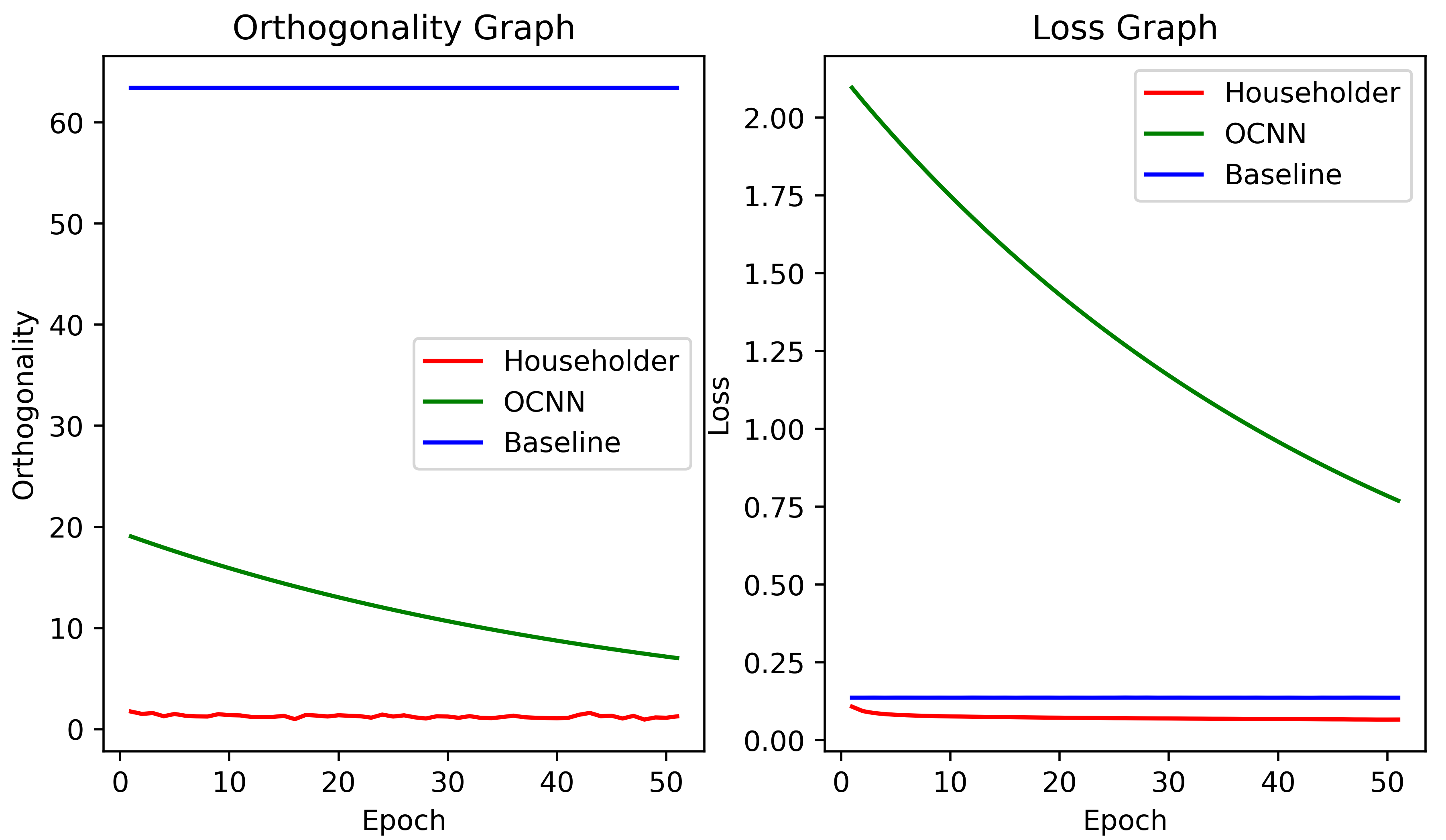
Figure 7: Capsnet with different Orthogonal regularization on MNIST dataset. Our HouseHolder orthogonalization method reaches better orthogonality and loss decay.

5 Conclusions and Future Work

In this study, we have introduced a novel capsule network with orthogonal sparse attention routing and pruning. Specifically, Householder orthogonal decomposition is used to ensure strict matrix orthogonality in attention routing without additional penalty terms, and the capsule pruning layer introduces sparsity into routing, minimizing capsule redundancies. Experiments show that OrthCaps has lower parameters and reduces computational overhead, overcoming the challenges of computational expense and redundancy in dynamic routing. On image classification tasks, OrthCaps outperforms state-of-the-art methods, demonstrating improved robustness. We look forward to further developments in this area.

Supplementary Material

6 Symbols and abbreviation used in this paper

Symbol	Description
OrthCaps	Orthogonal Capsule Network
OrthCaps-S	Shallow network variant of OrthCaps
OrthCaps-D	Deep network variant of OrthCaps
$x$	Input image
$l$	Layer index
$\Phi^{0}$	Features from initial convolutional layer
$u_{l,i}/(U_{l})$	Capsules/ (matrix) at layer $l$
$v_{l+1,i}/(V_{l+1})$	Capsules/ (matrix) at layer $l+1$
$n$	Capsule count in layer $l$
$m$	Capsule count in layer $l+1$
$d$	Capsule dimension
$W$	Feature map width
$H$	Feature map height
$B$	Batch size
$u_{flat}$	Flattened capsules
$u_{ordered}$	Capsules ordered by their $L_{2}$-norm
$u_{pruned}$	Pruned capsules
$m_{i}/(M)$	Mask column/matrix for pruned capsule layer
$t_{ij}/(T)$	Cosine similarities/ (matrix) for pruned capsule layer
$\theta$	Threshold for pruned capsule layer
$Q,K,V$	Attention routing components: Query, Key, Value
$W_{Q},W_{K},W_{V}$	Weight matrices for Q, K, V
$c_{i,j}/(C)$	Coupling coefficients/ (matrix) for attention routing
$s_{l+1,j}/(S_{l})$	Votes/ (matrix) for attention routing
$W$	Weight matrix for simplified attention routing
$g$	Activation function
$H$	Householder matrix
$a_{i}$	Unit vector in Householder matrix formulation
$b_{i}$	Learnable vector in Householder matrix

7 experimental Setups

7.1 hyperparameters

Hyperparameter	Value
Batchsize	512 (4 parallelled)
Learning rate	5e-3
Weight decay	5e-4
Optimizer	AdamW
Scheduler	CosineAnnealingLR and 5-cycle linear warm-up
Epochs	300
Data augmentation	RandomHorizonFlip, RandonClip with padding of 4
Dropout	0.25
$m^{+}$	0.9
$m^{-}$	0.1
$\lambda$	0.5
$\theta$	0.7
$d$	16

7.2 Setups

In this section, we describe the necessary Python library and corresponding version for the experiments in the main paper.

Library	Version
pytorch	1.12.1
numpy	1.24.3
opencv-python	4.7.0.72
pandas	2.0.2
pillow	9.4.0
torchvision	0.13.1
matplotlib	3.7.1
icecream	2.1.3
seaborn	0.12.0

8 HouseHolder Orthogonalization

8.1 Proof of Lemma 1

Assumption:

$V_{l+1}=\{v_{l+1,1},v_{l+1,2},\dots,v_{l+1,m}\}$ is a set of $m$ capsule vectors in layer $l+1$ of the network. $W$ is an orthogonal matrix, i.e. $W^{T}W=I$.

Proof:

we aim to prove that the cosine similarity $t_{ij}$ between any two capsules $v_{l+1,i}$ and $v_{l+1,j}$ remains constant after multiplied by $W$. For an orthogonal matrix $W$, the dot product and vector lengths are preserved. Let $\tilde{v}_{l+1,i}=Wv_{l+1,i}$, $\tilde{v}_{l+1,j}=Wv_{l+1,j}$ denote the transformed vectors. Thus, we have:

$$\tilde{v}_{l+1,i}\cdot\tilde{v}_{l+1,j} =(Wv_{l+1,i})^{T}(Wv_{l+1,j})$$ (7)

$$=v_{l+1,i}^{T}W^{T}Wv_{l+1,j}$$

$$=v_{l+1,i}^{T}v_{l+1,j}$$

and

$$\|\tilde{v}_{l+1,i}\|_{2} =\sqrt{(Wv_{l+1,i})^{T}(Wv_{l+1,i})}$$ (8)

$$=\sqrt{v}_{l+1,i}^{T}W^{T}Wv_{l+1,i}$$

$$=\sqrt{v}_{l+1,i}^{T}v_{l+1,i}$$

$$=\|v_{l+1,i}\|_{2}$$

Thus, we obtain transformed cosine similarity $\tilde{t}_{ij}$ in Eq. 9:

$$\tilde{t}_{ij} =\frac{(\tilde{v}_{l+1,i})\cdot(\tilde{v}_{l+1,j})}{\|\tilde{v}_{l+1,i}\|_{2}\|\tilde{v}_{l+1,j}\|_{2}}$$ (9)

$$=\frac{v_{l+1,i}\cdot v_{l+1,j}}{\|v_{l+1,i}\|_{2}\|v_{l+1,j}\|_{2}}$$

$$=t_{ij}$$

Therefore, orthogonal transformations preserve the cosine similarity between any two vectors.

8.2 Proof of Lemma 3

Proof:

Let $W$ represent one of $W_{Q}$,$W_{K}$,$W_{V}$ as $W$ can be expressed as

$$W=H_{0}H_{1}\dots H_{d-1}$$ (10)

where $H_{i}=I-2a_{i}a_{i}^{T}$. We have

$$W^{T}W=H_{d-1}^{T}\dots H_{1}^{T}H_{0}^{T}H_{0}H_{1}\dots H_{d-1}$$ (11)

We demonstrate that $H_{i}$ is orthogonal, i.e. $H_{i}^{T}H_{i}=I$. This is obvious, as

$$H_{i}^{T}H_{i} =(I-2a_{i}a_{i}^{T})^{T}(I-2a_{i}a_{i}^{T})$$ (12)

$$=I-4a_{i}a_{i}^{T}+4a_{i}a_{i}^{T}=I$$

Therefore, Equation (11) can be written as $W^{T}W=\underbrace{I\dots I}_{d}=I$.

8.3 Householder as a Regularization Technique

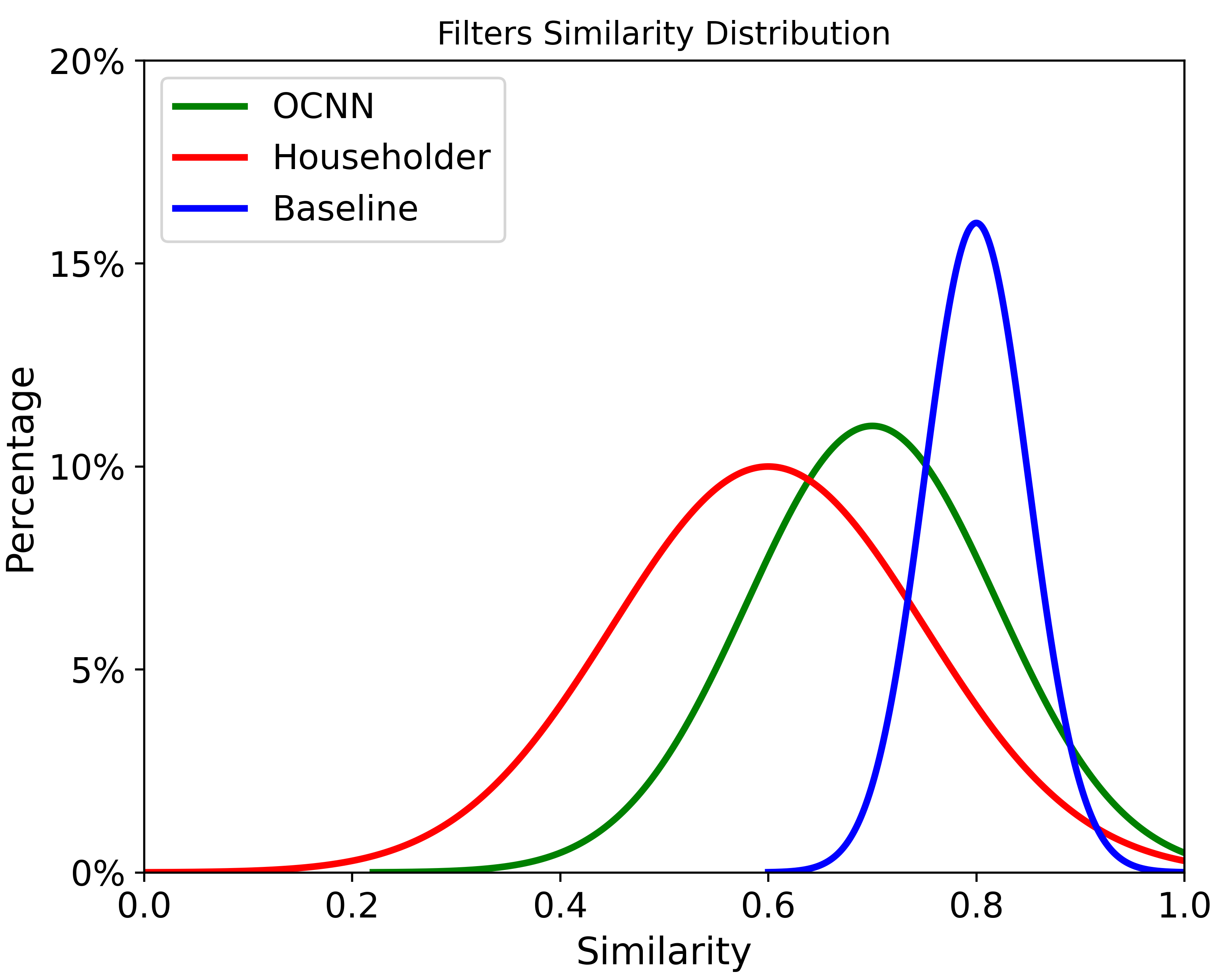
Figure 8: The normalized histogram of pairwise filter similarities in standard ResNet34 with different regularizers. HouseHolder orthogonalization method shows the best performance of descending filter similarity.

We demonstrate Householder’s role as a regularization technique for neural networks. For ResNet18, we flatten and concatenate convolutional kernels into a matrix $W$, and orthogonalize it to minimize off-diagonal elements, which reduces channel-wise filter similarity and redundancy. To quantify these properties, we used Guided Backpropagation to dynamically visualize the activations[36]. Compared to directly computing the covariance matrix of convolutional kernels, The gradient-based covariance matrix offers a more comprehensive view of the dynamic behavior of filters. We define the gradients from Guided Backpropagation as $G$ and compute its gradient correlation matrix $corr(G)$ as:

$$\left(\text{diag}(K_{GG})\right)^{-\frac{1}{2}}K_{GG}\left(\text{diag}(K_{GG})\right)^{-\frac{1}{2}}$$ (13)

where $K_{GG}=\frac{1}{M}\left((G-\mathbb{E}[G])(G-\mathbb{E}[G])^{T}\right)$, $M$ is the number of channels. Fig. 8 of the off-diagonal elements of $corr(G)$ shows a left-shifted distribution for the Householder-regularized model, confirming its effectiveness in enhancing filter diversity and reducing redundancy.

9 Dynamic Routing in Capsule Network

Algorithm 2 Dynamic Routing

procedure ROUTING($\hat{u}_{j|i}$, $r$, $l$)

       for all capsule $i$ in layer $l$ and capsule $j$ in layer $(l+1)$ do $b_{ij}\leftarrow 0$        

       for $T$ iterations do

             for all capsule $i$ in layer $l$ do $c_{i}\leftarrow\text{softmax}(b_{i})$              

             for all capsule $j$ in layer $(l+1)$ do $s_{j}\leftarrow\sum_{i}c_{ij}\hat{u}_{j|i}$              

             for all capsule $j$ in layer $(l+1)$ do $v_{j}\leftarrow\text{squash}(s_{j})$              

             for all capsule $i$ in layer $l$ and capsule $j$ in layer $(l+1)$ do $b_{ij}\leftarrow b_{ij}+\hat{u}_{j|i}\cdot v_{j}$                     

       return $v_{j}$

Algorithm 2 describes the dynamic routing algorithm. This algorithm allows lower-level capsule output vectors to be allocated to higher-level capsules based on their similarity, thereby achieving an adaptive feature combination. However, as evident from $\sum_{i}c_{ij}\hat{u}_{j|i}$, each higher-level capsule is a weighted sum of lower-level capsules. The higher-level capsules are fully connected with the lower level. Furthermore, the routing algorithm fundamentally serves as an unsupervised clustering process for capsules, requiring $r$ iterations to converge the coupling coefficients $c$. It’s crucial to strike a balance in choosing $r$: an inadequate number of iterations may hinder convergence of $c$, impairing routing efficacy, while an excessive count increases computational demands.

In Conclusion, it is crucial to introduce a straightforward, iterative-free routing algorithm.

References

- Chen et al. [2022] Hao Chen, Xian-bo Wang, and Zhi-Xin Yang. Fast robust capsule network with dynamic pruning and multiscale mutual information maximization for compound-fault diagnosis. IEEE/ASME Transactions on Mechatronics, 2022.
- Choi et al. [2019] Jaewoong Choi, Hyun Seo, Suii Im, and Myungjoo Kang. Attention routing between capsules. In Proceedings of the IEEE/CVF International Conference on Computer Vision (ICCV) Workshops, 2019.
- De Sousa Ribeiro et al. [2020] Fabio De Sousa Ribeiro, Georgios Leontidis, and Stefanos Kollias. Introducing routing uncertainty in capsule networks. In Advances in Neural Information Processing Systems, pages 6490–6502, 2020.
- Guo et al. [2019] Chuan Guo, Jacob Gardner, Yurong You, Andrew Gordon Wilson, and Kilian Weinberger. Simple black-box adversarial attacks. In Proceedings of the 36th International Conference on Machine Learning, pages 2484–2493. PMLR, 2019.
- He et al. [2016] Kaiming He, Xiangyu Zhang, Shaoqing Ren, and Jian Sun. Deep residual learning for image recognition. In Proceedings of the IEEE Conference on Computer Vision and Pattern Recognition (CVPR), pages 770–778, 2016.
- Hinton [2023] Geoffrey Hinton. How to represent part-whole hierarchies in a neural network. Neural Computation, 35(3):413–452, 2023.
- Hinton et al. [2018] Geoffrey E Hinton, Sara Sabour, and Nicholas Frosst. Matrix capsules with EM routing. In International Conference on Learning Representations, 2018.
- Hoogi et al. [2019] Assaf Hoogi, Brian Wilcox, Yachee Gupta, and Daniel L Rubin. Self-attention capsule networks for object classification. arXiv preprint arXiv:1904.12483, 2019.
- Huang et al. [2022] Huaibo Huang, Xiaoqiang Zhou, and Ran He. Orthogonal transformer: An efficient vision transformer backbone with token orthogonalization. Advances in Neural Information Processing Systems, 35:14596–14607, 2022.
- Huang et al. [2018] Lei Huang, Xianglong Liu, Bo Lang, Adams Yu, Yongliang Wang, and Bo Li. Orthogonal weight normalization: Solution to optimization over multiple dependent stiefel manifolds in deep neural networks. Proceedings of the AAAI Conference on Artificial Intelligence, 32(1), 2018.
- Huang et al. [2020] Lei Huang, Li Liu, Fan Zhu, Diwen Wan, Zehuan Yuan, Bo Li, and Ling Shao. Controllable orthogonalization in training DNNs. In Proceedings of the IEEE/CVF Conference on Computer Vision and Pattern Recognition (CVPR), pages 6429–6438, 2020.
- Huang and Zhou [2020] Wenkai Huang and Fobao Zhou. Da-capsnet: Dual attention mechanism capsule network. Scientific Reports, 10(1):11383, 2020.
- Jeong et al. [2019] Taewon Jeong, Youngmin Lee, and Heeyoung Kim. Ladder capsule network. In Proceedings of the 36th International Conference on Machine Learning, pages 3071–3079. PMLR, 2019.
- Krizhevsky [2009] Alex Krizhevsky. Learning multiple layers of features from tiny images. Technical report, University of Toronto, 2009.
- LeCun [1998] Yann LeCun. The MNIST database of handwritten digits. http://yann. lecun. com/exdb/mnist/, 1998.
- LeCun et al. [2004] Yann LeCun, Fu Jie Huang, and Léon Bottou. Learning methods for generic object recognition with invariance to pose and lighting. Technical report, Courant Institute of Mathematical Sciences, New York University, 2004.
- Li et al. [2020] Jun Li, Li Fuxin, and Sinisa Todorovic. Efficient riemannian optimization on the stiefel manifold via the cayley transform. arXiv preprint arXiv:2002.01113, 2020.
- Mathiasen et al. [2020] Alexander Mathiasen, Frederik Hvilshø j, Jakob Rø dsgaard Jø rgensen, Anshul Nasery, and Davide Mottin. What if neural networks had SVDs? In Advances in Neural Information Processing Systems, pages 18411–18420, 2020.
- Mazzia et al. [2021] Vittorio Mazzia, Francesco Salvetti, and Marcello Chiaberge. Efficient-capsnet: Capsule network with self-attention routing. Scientific Reports, 11(1):14634, 2021.
- Netzer et al. [2011] Yuval Netzer, Tao Wang, Adam Coates, Alessandro Bissacco, Bo Wu, and Andrew Y Ng. Reading digits in natural images with unsupervised feature learning. In NIPS Workshop on Deep Learning and Unsupervised Feature Learning 2011, 2011.
- Peng et al. [2020] Dunlu Peng, Dongdong Zhang, Cong Liu, and Jing Lu. Bg-sac: Entity relationship classification model based on self-attention supported capsule networks. Applied Soft Computing, 91:106186, 2020.
- Peters et al. [2019] Ben Peters, Vlad Niculae, and André FT Martins. Sparse sequence-to-sequence models. arXiv preprint arXiv:1905.05702, 2019.
- Pucci et al. [2021] Rita Pucci, Christian Micheloni, and Niki Martinel. Self-attention agreement among capsules. In Proceedings of the IEEE/CVF International Conference on Computer Vision (ICCV) Workshops, pages 272–280, 2021.
- Qi et al. [2020] Haozhi Qi, Chong You, Xiaolong Wang, Yi Ma, and Jitendra Malik. Deep isometric learning for visual recognition. In Proceedings of the 37th International Conference on Machine Learning, pages 7824–7835. PMLR, 2020.
- Rajasegaran et al. [2019] Jathushan Rajasegaran, Vinoj Jayasundara, Sandaru Jayasekara, Hirunima Jayasekara, Suranga Seneviratne, and Ranga Rodrigo. Deepcaps: Going deeper with capsule networks. In Proceedings of the IEEE/CVF Conference on Computer Vision and Pattern Recognition (CVPR), pages 10725–10733, 2019.
- Renzulli and Grangetto [2022] Riccardo Renzulli and Marco Grangetto. Towards efficient capsule networks. In 2022 IEEE International Conference on Image Processing (ICIP), pages 2801–2805. IEEE, 2022.
- Renzulli et al. [2022] Riccardo Renzulli, Enzo Tartaglione, and Marco Grangetto. Rem: Routing entropy minimization for capsule networks. arXiv preprint arXiv:2204.01298, 2022.
- Sabour et al. [2017] Sara Sabour, Nicholas Frosst, and Geoffrey E Hinton. Dynamic routing between capsules. In Advances in Neural Information Processing Systems, page 3856–3866, 2017.
- Sharifi et al. [2021] Ramin Sharifi, Pouya Shiri, and Amirali Baniasadi. Prunedcaps: A case for primary capsules discrimination. In 2021 20th IEEE International Conference on Machine Learning and Applications (ICMLA), pages 1437–1442. IEEE, 2021.
- Simonyan and Zisserman [2014] Karen Simonyan and Andrew Zisserman. Very deep convolutional networks for large-scale image recognition. arXiv preprint arXiv:1409.1556, 2014.
- Singla and Feizi [2021] Sahil Singla and Soheil Feizi. Skew orthogonal convolutions. In Proceedings of the 38th International Conference on Machine Learning, pages 9756–9766. PMLR, 2021.
- Trockman and Kolter [2021] Asher Trockman and J Zico Kolter. Orthogonalizing convolutional layers with the cayley transform. arXiv preprint arXiv:2104.07167, 2021.
- Tsai et al. [2020] Yao-Hung Hubert Tsai, Nitish Srivastava, Hanlin Goh, and Ruslan Salakhutdinov. Capsules with inverted dot-product attention routing. arXiv preprint arXiv:2002.04764, 2020.
- Uhlig [2001] Frank Uhlig. Constructive ways for generating (generalized) real orthogonal matrices as products of (generalized) symmetries. Linear Algebra and its Applications, 332:459–467, 2001.
- Virmaux and Scaman [2018] Aladin Virmaux and Kevin Scaman. Lipschitz regularity of deep neural networks: Analysis and efficient estimation. In Advances in Neural Information Processing Systems, pages 3835–3844, 2018.
- Wang et al. [2020] Jiayun Wang, Yubei Chen, Rudrasis Chakraborty, and Stella X. Yu. Orthogonal convolutional neural networks. In Proceedings of the IEEE/CVF Conference on Computer Vision and Pattern Recognition (CVPR), pages 11505–11515, 2020.
- Xiao et al. [2017] Han Xiao, Kashif Rasul, and Roland Vollgraf. Fashion-MNIST: A novel image dataset for benchmarking machine learning algorithms. arXiv preprint arXiv:1708.07747, 2017.
- Yang et al. [2020] Shuai Yang, Feifei Lee, Ran Miao, Jiawei Cai, Lu Chen, Wei Yao, Koji Kotani, and Qiu Chen. Rs-capsnet: An advanced capsule network. IEEE Access, 8:85007–85018, 2020.