Forecasting density-valued functional panel data
Abstract
We introduce a statistical method for modeling and forecasting functional panel data, where each element is a density. Density functions are nonnegative and have a constrained integral and thus do not constitute a linear vector space. We implement a center log-ratio transformation to transform densities into unconstrained functions. These functions exhibit cross-sectionally correlation and temporal dependence. Via a functional analysis of variance decomposition, we decompose the unconstrained functional panel data into a deterministic trend component and a time-varying residual component. To produce forecasts for the time-varying component, a functional time series forecasting method, based on the estimation of the long-range covariance, is implemented. By combining the forecasts of the time-varying residual component with the deterministic trend component, we obtain -step-ahead forecast curves for multiple populations. Illustrated by age- and sex-specific life-table death counts in the United States, we apply our proposed method to generate forecasts of the life-table death counts for 51 states.
Keywords: Compositional data analysis; Constrained functional time series; Density function forecasting; Functional median polish; Functional analysis of variance
1 Introduction
Actuaries and demographers are interested in developing models for mortality forecasting (see, e.g., Booth, 2006; Booth and Tickle, 2008; Basellini et al., 2023, for comprehensive reviews). From an actuary perspective, mortality forecasts are important inputs in determining fixed-term or lifetime annuities. They are important to manage the financial effects of mortality improvements over time on pensions (Pollard, 1987) and are essential to the financial viability of life insurance companies. From a demography perspective, mortality forecasts are essential to health and aged-care systems (see, e.g., Shang et al., 2016) and are an important component of population forecasts (see, e.g., Hyndman et al., 2021) for urban and rural planning.
For modeling age-specific mortality, three functions related to mortality are commonly studied: hazard function, survival function, and life-table death counts. Hazard functions are bounded between 0 and 1. The survival function monotonically decreases. The life-table death counts of each age group are non-negative and sum to a radix of each year, which strongly resembles probability density functions (PDFs). Among these three functions, life-table death counts provide important insights into longevity risk and lifespan variability that cannot be easily quantified from either hazard or survival function. These additional constraints on the life-table death counts can be helpful to improve forecast accuracy (see, e.g., Oeppen, 2008; Bergeron-Boucher et al., 2017; Basellini et al., 2020; Pascariu et al., 2019). For instance, in many developed countries, deaths at younger ages gradually shift toward older ages. In addition to providing an informative description of the mortality experience of a population, the life-table death counts yield readily available information on ”central longevity indicators”, that is, mean, median, and mode age at death (Canudas-Romo, 2010), and lifespan variability (Robine, 2001; Vaupel et al., 2011; van Raalte and Caswell, 2013; van Raalte et al., 2014). For many developed countries, a decrease in variability over time may be observed through the Gini coefficient of life-table ages at death (Shang et al., 2022) or Drewnowski’s index (Aburto et al., 2022).
Because of the two constraints, life-table death counts can be viewed as compositional data. Compositional data are defined as a random vector of compositions , non-negative values in which the sum of is a given constant, typically one (portions) in probability density function (Kokoszka et al., 2019), 100 (%) in weekly household expenditure (Scealy and Welsh, 2017), and for parts per million in geochemical compositions (see, e.g., Scealy et al., 2015). The sample space of compositional data is a (nonlinear) simplex
| (1) |
where denotes life-table death count for age , where and denotes the total number of discrete ages, is a fixed constant, and ⊤ denotes vector transpose.
In compositional data analysis, there exist several transformations from the simplex to Euclidean space. Among them, the center log ratio (clr) is the simplest and most widely used transformation because principal component analysis (PCA) is not invariant to general linear affine transformations (Aitchison, 1982). For a given year , the clr transformation is defined as
| (2) |
where denotes natural logarithm, for . From a time series of , Bergeron-Boucher et al. (2017) applied a principal component analysis (PCA) to extract latent principal components and their associated scores. The scores can be modeled and forecast using a univariate time series forecasting method. With the forecast principal component scores, can be obtained with the estimated principal components. By taking the inverse clr transformation, can be estimated by
where is the radix reported in the Human Mortality Database (2024).
Extending these works, we develop statistical models to jointly forecast life-table death counts as a function of age at the sub-national level. Understanding patterns in mortality across subpopulations is essential for local health policy decision-making, identifying mortality patterns of vulnerable groups, classifying heterogeneous populations into homogeneous groups, and tracking the effects of policy responses. The series at the sub-national level presents two challenges: (1) the signal-to-noise ratio is comparably low; and (2) the number of series may exceed the number of curves in a series. The latter leads to the study of high-dimensional functional time series (HDFTS) (see, e.g., Fang et al., 2022; Elías et al., 2023; Guo and Qiao, 2023; Chang et al., 2024; Jiménez-Varón et al., 2024; Tan et al., 2024).
In the context of high-dimensional functional time series (HDFTS), Zhou and Dette (2023) derived Gaussian and multiplier bootstrap approximations for sums of HDFTS. These approximations were utilized to construct joint simultaneous confidence bands for the mean functions and develop a hypothesis test to assess the parallel behavior of the mean functions in the panel dimension. Hallin et al. (2023) investigated the representation of HDFTS using a factor model, identifying crucial conditions on the eigenvalues of the covariance operator for the existence and uniqueness of the factor model. Gao et al. (2019) adopted a two-stage approach, combining truncated principal component analysis and a separate scalar factor model for the resulting panels of scores. In contrast, Tavakoli et al. (2023) introduced a functional factor model with a functional factor loading and a vector of real-valued factors, while Guo et al. (2022) considered a functional factor model with a real-valued factor loading and a functional factor. Additionally, Tang et al. (2022) studied clustering problems for age-specific mortality rates as an example of HDFTS, and Li et al. (2024) proposed hypothesis tests for detecting and identifying change points, and clustering of change points in HDFTS using an information criterion.
In the realm of estimating HDFTS models, Guo and Qiao (2023) introduced a three-step procedure that incorporates a novel functional stability measure, the non-asymptotic properties of functional principal component analysis (FPCA), and a regularization approach for estimating autoregressive coefficients. Moreover, Tan et al. (2024) proposed dynamic weak separability to characterize the two-way dependence structure in multivariate functional time series, developing a unified framework for functional graphical models and dynamic principal component analysis. Chang et al. (2024) presented a three-step framework for statistical learning of HDFTS with errors, incorporating autocovariance-based dimension reduction and a novel block regularized minimum distance estimation.
In practice, it is common to find functional objects that do not reside in a linear Hilbert space. This is exemplified by various scenarios, such as analyzing time series consisting of probability density functions (PDFs) and cumulative density functions (CDFs). In the context of PDFs, the works of Kneip and Utikal (2001) and Shang et al. (2022) have studied the age distribution of death counts. Specifically, for life table death counts, Pascariu et al. (2019) have proposed a forecasting method that utilizes the location and shape measures of density functions. Moreover, in nonstationary time series, Chang et al. (2016) have considered modeling state densities, while Horta and Ziegelmann (2018) have explored the dynamics of financial return densities. In terms of CDFs, Condino (2023) have examined a sequence of Lorenz curves derived from a regional household income and wealth survey in Italy. Zhang et al. (2024) proposed a functional ridge-regression-based estimation method that estimates cumulative distribution functions accurately everywhere. We aim to introduce a forecasting method for HDFTS where the functional objects are PDFs.
When the functional objects are nonlinear, it is common to transform the functional objects into a linear space. A popular space is the Bayes Hilbert space studied in Hron et al. (2016) and Seo and Beare (2019). Hron et al. (2016) introduced the simplicial functional principal component analysis of densities. Simplicial functional principal component analysis is based on the geometry of the Bayes space of functional compositions. It utilizes the centered log-ratio transformation to map the densities to a suitable Hilbert space, enabling the application of standard functional data analytic techniques. Seo and Beare (2019) focused on modeling nonstationary time series of probability density functions. They illustrated the isomorphism between a cointegrated Bayes Hilbert space and a cointegrated linear process in a Hilbert space of centered square-integrable real functions.
A unique feature associated with the HDFTS is that they can be cross-sectionally correlated and temporally dependent. We deploy a two-way functional analysis of variance (ANOVA), as used by Jiménez-Varón et al. (2024) to decompose HDFTS into a deterministic trend component and a residual component that varies over time. These components can be estimated by functional median polish decomposition (FMP-ANOVA) and functional analysis of variance based on means (FM-ANOVA). Both decompositions compute the functional grand effect and functional main factor effects in an additive model without factor interaction. The FM-ANOVA has been extensively studied by Zhang (2014). The FMP-ANOVA was proposed by Sun and Genton (2012) as an extension of the univariate median polish of Tukey (1977) and Mosteller and Tukey (1977). It is a robust statistical technique for studying the effects of factors on the response since it replaces the mean with the median (Emerson and Hoaglin, 1983). The proposed FTS forecasting method for densities is compared with existing methods, such as the factor models from Gao et al. (2019) and Tavakoli et al. (2023), and the maximum entropy mortality model proposed by Pascariu et al. (2019).
In the two-way functional ANOVA, Jiménez-Varón et al. (2024) forecast the time-varying residual component using a functional time series forecasting approach based on FPCA. Prediction intervals were then provided using a sieve bootstrap procedure introduced by Paparoditis and Shang (2023). While Jiménez-Varón et al. (2024) considered the unbounded log mortality rates, we focus on life-table death counts constrained by non-negativity and summability.
The remainder of this paper is structured as follows. In Section 2, we present the United States (US) sub-national mortality rates across 51 states. In Section 3, we apply functional ANOVA decomposition to extract a deterministic trend component and a time-varying residual component. For modeling and forecasting the residual component, we introduce a functional time series forecasting method based on functional principal component analysis (FPCA) for producing forecasts. By combining the time-varying component forecasts with the deterministic component, we obtain -step-ahead forecast curves for multiple populations. With the inverse clr transformation, we transform our forecast curves back to the simplex. In doing so, we obtain forecast life-table death counts. We evaluate and compare point and interval forecast accuracies in Sections 4.1 and 4.4, respectively. Section 5 concludes and offers some ideas on how the methodology presented can be further extended.
2 Age distribution of life-table death counts in the United States
We consider US age- and sex-specific life-table death counts from 1959 to 2020, obtained from the United States Mortality Database (2024). The database documents a historical set of complete state-level life tables designed to foster research on geographic variations in mortality across the US and monitor trends in health inequalities. This data set includes complete and abridged life tables by sex for each of the nine Census Divisions, four Census Regions, 50 States of the US, as well as the District of Columbia, with mortality up to age 110.
The life-table radix is fixed at at age 0 for each year. For the life-table death counts, there are 111 ages, and these are age . Due to rounding, there may be zero counts, especially for older ages at some years. To rectify the problem, one can also use the probability of dying (i.e., ) and the life-table radix to recalculate the estimated death counts with decimal places. The smoother estimates are more detailed than those reported in the United States Mortality Database (2024).
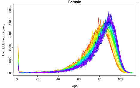
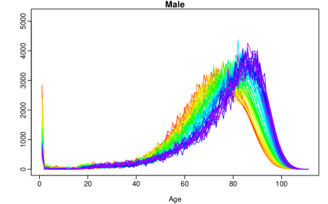
To understand the primary features of the data, Figures 1a and 1b present rainbow plots of the female and male age-specific life-table death counts in Rhode Island in a single-year group. The time ordering of the curves follows the colors of the rainbow, where data from the distant past are shown in red and more recent data are shown in purple. Both figures demonstrate a decreasing trend in infant mortality and a negatively skewed distribution for the life-table death counts, where the peaks shift to older ages for both females and males. The shift of the distribution symbolizes longevity risk, which can be a major issue for insurers and government pensions, especially in the selling and risk management of annuities (see Brouhns et al., 2002; Canudas-Romo, 2010, for discussion).
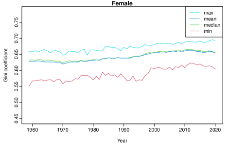
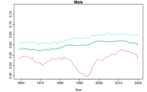
The Gini coefficient is a measure that quantifies the level of inequality in age at death within a life table population. A lower Gini coefficient value indicates less age variability at death, suggesting a greater level of equality (Basellini et al., 2020; Aburto et al., 2022). In Figure 2, we present the Gini coefficient for the US for the female population (left) and male population (right). We can observe from both figures that, on average, there has been an increasing trend in the Gini coefficient over the years. The observed increasing tendency can be explained by a continuous decrease in the ratio between the resulting life expectancy at birth when doubling the hazard at all ages and the overall life expectancy at birth (Aburto et al., 2022).
3 Methodology
The life-table death counts are discrete and densely observed. By adopting the linear interpolation algorithm of Hyndman et al. (2023), we convert them into a continuous function on the same function support .
3.1 Center log-ratio transformation for density-valued functional time series
Let be the age-specific life-table death count for age , state , gender at year . For a given year , compositional data are defined as a random vector of non-negative components, and the sum of which is a specified constant. Between the non-negativity and summability constraints, the sample space of functional compositional data is a simplex of the form in (1).
When age is treated as a continuum, the clr transformation in (2) can be written as
where denotes the length of the age interval, and is the geometric mean. When considering life-table death counts as density curves, Shang and Haberman (2020) and Shang et al. (2022) developed a functional principal component regression to forecast a time series of density curves in the constrained space. Via the inverse clr transformation, the forecast life-table death counts can be obtained as
3.2 Two-way functional ANOVA model
Let be the transformed data for age , state , gender at year . By treating age as a continuum, a two-way functional ANOVA decomposition can be expressed as:
| (3) |
where denotes the functional grand effect, denotes the functional row effect, and, denotes the functional column effect. For each state and gender , we considered replicates for the years with time horizon, for , , and . denotes the residual component that varies over time for the state and gender . Such a decomposition is not an approximation and can exactly reconstruct the original data.
The model described in (3), can be estimated in two ways: the FM-ANOVA approach (Zhang, 2014; Ramsay and Silverman, 2006) or FMP-ANOVA approach (Sun and Genton, 2012). The former extracts the deterministic component into the following terms:
There exist some identifiability constraints, so that for all , , and for all (Ramsay and Silverman, 2006, Chapter 13). The FMP-ANOVA decomposition satisfies that , , , for all (Sun and Genton, 2012).
3.3 Point forecasts based on functional analysis of variance
For the functional residual process obtained from either the FMP-ANOVA or FM-ANOVA, we consider a functional time series forecasting method based on the FPCA of Shang (2019). The proposed FPCA relies on an accurate estimate of the long-run covariance function, for which we consider a kernel sandwich estimator with plug-in bandwidth (see, e.g., Horváth et al., 2016; Rice and Shang, 2017).
For a given state and gender , denote as a stationary ergodic functional time series exhibiting stationarity and ergodicity. In essence, the statistical features of a stochastic process will not vary over time, and they can be obtained from a single, sufficiently long sample of the process. For such a random process, the long-run covariance function can be defined as
where and denote a lag variable.
While the long-run covariance can be expressed as a bi-infinite summation, its estimation is not trivial. For a finite sample, a natural estimator of is
| (4) |
where
The long-run covariance function in (4) can be seen as a sum of autocovariance functions with decreasing weights. It is common in practice to determine the optimal lag value of to balance the trade-off between squared bias and variance. In Li et al. (2020), is the minimum between sample size and the number of discretized points in a function. Other approaches use the kernel sandwich estimator as in Horváth et al. (2016)
where is the bandwidth parameter, and is a symmetric weight function with bounded support of order . Rice and Shang (2017) propose a plug-in algorithm for obtaining the optimal bandwidth parameter to minimize the asymptotic mean-squared normed error between the estimated and theoretical long-run covariance functions.
Via Mercer’s lemma (Mercer and Forsyth, 1909), the estimated long-run covariance function can be approximated by
where are the eigenvalues of , and are the orthonormal functional principal components. We can project a functional time series onto a set of orthogonal functional principal components via the inner product in the corresponding Hilbert space. This leads to the Karhunen-Loève expansion of the realization of a stochastic process,
where , denotes the set of principal component scores for time , denotes the number of retained components, and denotes the error term with zero mean and finite variance.
There are various ways to determine the value of : (1) scree plots or the fraction of variance explained by the first few functional principal components (Chiou, 2012); (2) pseudo-versions of Akaike information criterion and Bayesian information criterion (Yao et al., 2005); (3) predictive cross validation leaving out one or more curves (Ramsay and Silverman, 2006); (4) bootstrap methods (Hall and Vial, 2006); and (5) eigenvalue ratio criterion (Ahn and Horenstein, 2013; Li et al., 2021). Here, we select via the eigenvalue ratio criterion (EVR) of Li et al. (2021). The value of is determined as the integer minimizing ratio of two adjacent empirical eigenvalues given by
| (5) |
where is a pre-specified small positive number, set as , and is the binary indicator function. is a pre-specified positive integer, we choose , as follows
where denotes the cardinality of the set.
Because the female and male populations within a state can exhibit a strong dependence, we utilize a multivariate FPCA. For a given state , collectively modeling multiple populations requires truncating numbers of functional principal components of joint time series
where , F and M denote the female and male populations in a given state, and
is a vector of principal component scores. is a matrix that contains the associated basis functions. By conditioning on , we obtain the -step-ahead point forecasts as follows
where represents the joint mean function.
A univariate time series method can be implemented to produce the forecasts of the principal component scores. The most commonly used methods are the exponential smoothing and autoregressive integrated moving average (ARIMA) models. For determining the forecast principal component score, we apply the univariate time series forecasting method of Hyndman and Shang (2009) based on the ARIMA approach (see also Shang and Hyndman, 2017; Shang and Yang, 2021; Jiménez-Varón et al., 2024). Because the age-specific life-table death counts are observed yearly, the ARIMA takes the generic form of
| (6) |
where represents the intercept, denote the coefficients associated with the autoregressive component, represents the principal component score, denote the coefficients associated with the moving average component, denotes the backshift operator, denotes the differencing operator, and represents a white-noise error term. The automatic selection method of Hyndman and Khandakar (2008) chooses the optimal autoregressive order p, moving average order q, and difference order . The value of is chosen using the Kwiatkowski-Phillips-Schmudt-Shin (KPSS) unit root tests (Kwiatkowski et al., 1992).
Once the forecasted functional residuals are obtained, we add the deterministic component from the FMP-ANOVA decomposition. As this is not time-varying, the overall -step-ahead point forecast is defined as
where is defined in (3). Then, we transform back to the original scale through the inverse clr transformation in Section 3.1.
3.4 Construction of prediction intervals
Prediction intervals are valuable for evaluating the probabilistic uncertainty associated with point forecasts. The forecast uncertainty stems from systematic deviations (e.g., due to parameter or model uncertainty) and random fluctuations (e.g., due to model error term). As was emphasized by Chatfield (1993, 2000), it is important to provide prediction intervals as well as point forecasts to: (1) assess future uncertainty levels; (2) enables different strategies to be planned for a range of possible outcomes indicated by the interval forecasts; (3) compare forecasts from different methods more thoroughly; and (4) explore different scenarios based on various assumptions.
We aim to construct a prediction interval for the constrained functional residuals . Let us consider the unconstrained functional time series with the corresponding functional residuals and the deterministic components . The bootstrap prediction intervals are constructed as follows.
-
1)
Compute the long-run covariance function for the time-varying residual component .
-
a)
From the eigenvalue ratio criterion in (5), determine the number of principal components . Via the multivariate FPCA, the functional principal component scores are computed by
-
b)
Using a univariate time series method described in (6), obtain the -step-ahead forecast for the principal component scores .
-
c)
Using the same univariate time series method described in (6), obtain the in-sample forecast for the principal component scores, denoted as for .
-
d)
Compute the in-sample forecast error associated with the principal component scores, as follows,
-
e)
Obtain bootstrap forecasts of principal component scores,
where represents the bootstrap samples of the in-sample forecast error in step 1d.
-
a)
-
2)
Compute model residuals from the multivariate FPCA for the time-varying residual component ,
where denotes the fitted functional time series.
-
3)
Bootstrap the model residuals by sampling with replacement from .
-
4)
By combining the two sources of errors, we obtain bootstrap forecasts of the residual component
-
5)
Obtain the bootstrap prediction , by adding the deterministic component from the functional ANOVA decomposition in §3.2, the bootstrap forecasts of the residual component. The bootstrap predictions are generated as follows:
(7) -
6)
Transform the bootstrap predictions in (7) back to the original constrained space by using the inverse clr transformation. The transformed bootstrap predictions are as follows,
(8) -
7)
For a level of significance , take and quantile levels from the transformed bootstrapped predictions in (8).
4 Forecast accuracy evaluation of life-table death counts
The forecasting methods based on FMP-ANOVA and FM-ANOVA are applied to the age- and sex-specific life-table death counts for the US.
4.1 Point forecast evaluation
We consider a rolling-window scheme to assess the point forecast as described in Zivot and Wang (2006, Chapter 9). The procedure is carried out as follows.
-
1)
The transformed data are decomposed, through the two-way FMP-ANOVA and FM-ANOVA in Section 3.2, into deterministic and time-varying components. The two factors are the state and gender (males and females). The functional residual curves are those obtained after removing all deterministic components.
-
2)
We perform an -step-ahead point forecast of the time-varying component. Then, we add the deterministic components to obtain the point forecast of the future curves.
-
3)
To compute each of the -step-ahead point forecasts, for , we proceed as follows: we consider a rolling window as a training set of size and produce a -step-ahead point forecast.
-
4)
The process iterates from to , where the training data set with equal sample size rolls one-step-ahead each time.
-
5)
With the holdout densities, we compute the point and interval forecast errors.
Since the sub-national age-specific life-table death counts can be considered a probability density function, we consider some density evaluation measures to evaluate the point forecast accuracy. These metrics include the discrete version of the Kullback-Liebler divergence (Kullback and Leibler, 1951) and the square root of the Jensen-Shannon divergence (Shannon, 1948). The Kullback-Liebler divergence is intended to measure the loss of information when we choose an approximation. For two probability density functions denoted by and , the discrete version of the Kullback-Liebler divergence is defined as
which is symmetric and non-negative. An alternative is given by the Jensen-Shannon divergence defined by
where measures a common quantity between and (Fuglede and Topsøe, 2004). We consider geometric mean given by .
We report the averaged KLD and JSD across number of states. That is,
The average across the forecast horizons for both KLD and JSD can be computed as follows,
4.2 Point forecast comparison
The obtained results for the point forecast accuracy for the US, using the EVR criterion described in (5), are provided in Table LABEL:tab:1. We present the KLD and across the forecast horizon averaged across states for each country and gender. We incorporate the accuracy mean over the forecast horizon. In Appendix A we conduct additional sensitivity analysis by fixing the number of functional principal components to as advocated by Hyndman et al. (2013).
| FMP-ANOVA | FM-ANOVA | |||||||
|---|---|---|---|---|---|---|---|---|
| Female | Male | Female | Male | |||||
| KLD | JSDg | KLD | JSDg | KLD | JSDg | KLD | JSDg | |
| 1 | 1.83 | 0.52 | 2.17 | 0.59 | 1.17 | 0.33 | 1.36 | 0.36 |
| 2 | 1.83 | 0.52 | 2.24 | 0.61 | 1.22 | 0.34 | 1.41 | 0.38 |
| 3 | 1.93 | 0.53 | 2.35 | 0.64 | 1.31 | 0.37 | 1.51 | 0.40 |
| 4 | 2.11 | 0.58 | 2.54 | 0.68 | 1.47 | 0.40 | 1.66 | 0.44 |
| 5 | 2.34 | 0.64 | 2.75 | 0.73 | 1.67 | 0.46 | 1.85 | 0.49 |
| 6 | 2.64 | 0.72 | 3.04 | 0.80 | 1.92 | 0.52 | 2.11 | 0.55 |
| 7 | 2.98 | 0.82 | 3.33 | 0.88 | 2.19 | 0.59 | 2.35 | 0.61 |
| 8 | 3.33 | 0.90 | 3.71 | 0.98 | 2.53 | 0.67 | 2.68 | 0.70 |
| 9 | 4.58 | 1.37 | 4.14 | 1.09 | 3.18 | 0.86 | 3.08 | 0.80 |
| 10 | 6.04 | 1.60 | 5.56 | 1.45 | 4.84 | 1.25 | 4.47 | 1.14 |
| Mean | 2.66 | 0.75 | 3.18 | 0.85 | 1.95 | 0.53 | 2.28 | 0.59 |
From the results in Table LABEL:tab:1, the proposed FM-ANOVA method generally outperforms the FMP-ANOVA method. The FM-ANOVA method consistently achieves lower values for KLD and . Additionally, the accuracy of point forecasts shows an increasing trend as the forecast horizon extends. When comparing the two proposed methods, the forecast errors for the female population are generally lower than that for the male population.
4.3 Competitive HDFTS forecasting methods
We discuss alternative methods from the recent HDFTS literature. For the methods introduced by Gao et al. (2019) and Tavakoli et al. (2023), we incorporate the clr transformation to ensure that the density functions belong to the same functional space during modeling and forecasting. However, the method proposed by Pascariu et al. (2019) does not require transformation, as it is designed to work directly with densities. In Appendix B, we also included the results of the two alternative methods without the clr transformation.
4.3.1 Two-stage functional principal component analysis
Gao et al. (2019) adopted a two-stage approach combining truncated principal component analysis and a separate scalar factor model for the resulting panels of scores. Their method consists of three steps.
-
1)
Dynamic FPCA is performed separately on each set of functional time series, resulting in sets of principal component scores of low dimension .
-
2)
The first functional principal component scores from each of sets of functional time series are combined into an vector. We fit factor models to the FPC scores to further reduce the dimension into an vector, where . The same procedure is implemented for the second, third, and so on until the th FPC scores. The vector of functional time series is reduced to an matrix.
-
3)
A scalar time series model can be fitted to each factor and forecasts are produced. The forecast factors can be used to construct forecast functions.
4.3.2 Functional factor model
Tavakoli et al. (2023) introduce the following functional factor model:
where is the functional factor loading and is a vector of real-valued factors.
4.3.3 Maximum entropy mortality model
In the demographic literature, several attempts exist to model the age distribution of death counts. Pascariu et al. (2019) propose matching finite (typically, the first four) statistical moments of the age distribution of death counts. The forecast life-table death counts for a population can be determined by extrapolating these moments. The extrapolation is achieved through multivariate time series models, such as multivariate random walk with drift. With the forecast moments, the forecast age distribution of death counts is then obtained.
Table LABEL:tab:1_new provides an evaluation and comparison of the point forecast accuracy for three competitive methods. In the case of the methods proposed by Tavakoli et al. (2023) and Gao et al. (2019), the CoDa transformation is applied, as these methods were not originally designed for density-valued functions. To emphasize the significance of the CoDa transformation, we also present the point forecast results of these two methods without the transformation in Appendix B.
| TNH23 | GSY19 | PLC19 | ||||||||||
|---|---|---|---|---|---|---|---|---|---|---|---|---|
| Female | Male | Female | Male | Female | Male | |||||||
| KLD | JSDg | KLD | JSDg | KLD | JSDg | KLD | JSDg | KLD | JSDg | KLD | JSDg | |
| 1 | 1.00 | 0.28 | 0.93 | 0.25 | 6.84 | 1.77 | 7.58 | 1.90 | 2.38 | 0.52 | 1.89 | 0.66 |
| 2 | 1.04 | 0.29 | 1.01 | 0.27 | 8.97 | 2.41 | 9.71 | 2.39 | 2.38 | 0.52 | 1.92 | 0.66 |
| 3 | 1.10 | 0.30 | 1.15 | 0.31 | 7.68 | 1.96 | 9.60 | 2.50 | 2.42 | 0.55 | 2.02 | 0.67 |
| 5 | 1.29 | 0.35 | 1.51 | 0.40 | 7.94 | 2.07 | 9.04 | 2.34 | 2.51 | 0.58 | 2.14 | 0.69 |
| 5 | 1.21 | 0.33 | 1.34 | 0.36 | 11.53 | 3.24 | 10.68 | 2.76 | 2.57 | 0.62 | 2.31 | 0.71 |
| 6 | 1.40 | 0.38 | 1.72 | 0.45 | 9.54 | 2.42 | 8.85 | 2.23 | 2.83 | 0.70 | 2.61 | 0.78 |
| 7 | 1.54 | 0.42 | 1.97 | 0.51 | 9.18 | 2.32 | 9.38 | 2.34 | 2.91 | 0.75 | 2.84 | 0.79 |
| 8 | 1.72 | 0.46 | 2.24 | 0.58 | 14.21 | 3.92 | 10.07 | 2.53 | 3.25 | 0.82 | 3.13 | 0.88 |
| 9 | 2.02 | 0.54 | 2.64 | 0.69 | 12.46 | 3.13 | 9.42 | 2.36 | 3.72 | 1.00 | 3.80 | 1.01 |
| 10 | 2.90 | 0.75 | 3.52 | 0.90 | 12.03 | 3.12 | 11.11 | 2.85 | 4.78 | 1.33 | 5.15 | 1.26 |
| Mean | 1.52 | 0.41 | 1.80 | 0.47 | 10.04 | 2.64 | 9.54 | 2.42 | 2.97 | 0.74 | 2.78 | 0.81 |
Although the functional factor model introduced by Tavakoli et al. (2023) achieves the highest accuracy in terms of point forecasts among all the methods, the difference is not substantial when compared to our proposed FM-ANOVA. Our approach offers the added advantage of providing prediction intervals for uncertainty quantification, which is not yet incorporated in Tavakoli et al.’s (2023) model.
Because of the two-stage FPCA, the method of Gao et al. (2019) suffers information loss and can result in the worst accuracy among the three competitors. The maximum entropy model of Pascariu et al. (2019) was designed for modeling the age distribution of death counts. Hinging on the existence of finite statistical moments, it provides moderate point forecast accuracy.
4.4 Interval forecast evaluation
To evaluate pointwise interval forecast accuracy, we consider the coverage probability difference (CPD) between the nominal and empirical coverage probabilities (ECP). The empirical coverage probability is defined as follows
where denotes the number of discretized points for the age, and denote the upper and lower bounds of the corresponding forecasted interval in the specific period. The pointwise CPD is defined as
The lower the CPD value, the better the forecasting method’s performance.
Additionally, we utilize the interval score (IS) of Gneiting and Raftery (2007) (see also Gneiting and Katzfuss, 2014, for a detailed review). For each year in the forecasting period, the -step-ahead prediction intervals were calculated at the nominal coverage probability. We consider the common case of the symmetric prediction interval, with lower and upper bounds that are predictive quantiles at and , denoted by and . The scoring rule for the interval forecast at discretized point is
where denotes a level of significance. We compute the mean interval score across states for a specific forecast horizon as follows,
The optimal interval score is achieved when lies between and , with the distance between the upper bound and the lower bound being minimal.
4.5 Interval forecast comparison
We present the obtained results for the interval forecast accuracy for scenarios in the US in Table LABEL:tab:2 for nominal coverage probabilities of and . We report the ECP, CPD, and IS (Gneiting and Raftery, 2007) for each method and gender within the forecast horizon averaged across states. We take into account the accuracy mean for the forecast period. Overall, considering all the metrics used, it is observed that the interval forecast errors tend to increase as the prediction horizon extends. This pattern holds for both functional ANOVA decompositions and across genders. Specifically, the female population is more likely to achieve a greater empirical coverage probability (ECP) than the male population. There is a general tendency for undercoverage in the male population, reflecting the difficulty of modeling populations with greater variability.
| FMP-ANOVA | FM-ANOVA | ||||||||||||
|---|---|---|---|---|---|---|---|---|---|---|---|---|---|
| Female | Male | Female | Male | ||||||||||
| Nominal | ECP | CPD | IS | ECP | CPD | IS | ECP | CPD | IS | ECP | CPD | IS | |
| 80% | 1 | 81.66 | 5.38 | 0.56 | 68.84 | 13.48 | 0.61 | 81.61 | 5.44 | 0.56 | 68.79 | 13.51 | 0.60 |
| 2 | 81.08 | 5.29 | 0.57 | 67.51 | 14.49 | 0.62 | 81.18 | 5.34 | 0.57 | 67.39 | 14.51 | 0.62 | |
| 3 | 80.07 | 5.35 | 0.59 | 65.56 | 16.21 | 0.65 | 80.19 | 5.43 | 0.59 | 65.47 | 16.23 | 0.65 | |
| 4 | 78.85 | 5.90 | 0.61 | 63.09 | 18.65 | 0.68 | 78.72 | 5.87 | 0.61 | 63.02 | 18.58 | 0.68 | |
| 5 | 77.18 | 6.72 | 0.63 | 60.94 | 20.56 | 0.71 | 77.28 | 6.68 | 0.63 | 60.83 | 20.63 | 0.71 | |
| 6 | 76.05 | 7.85 | 0.66 | 59.10 | 22.29 | 0.74 | 76.12 | 7.71 | 0.66 | 58.96 | 22.32 | 0.73 | |
| 7 | 75.32 | 8.45 | 0.69 | 57.64 | 23.69 | 0.77 | 75.18 | 8.42 | 0.69 | 57.56 | 23.71 | 0.77 | |
| 8 | 73.76 | 10.02 | 0.71 | 55.86 | 25.07 | 0.82 | 73.67 | 9.93 | 0.71 | 55.34 | 25.55 | 0.82 | |
| 9 | 70.41 | 12.52 | 0.76 | 52.09 | 28.92 | 0.90 | 70.47 | 12.38 | 0.76 | 51.70 | 29.23 | 0.90 | |
| 10 | 60.25 | 21.78 | 0.90 | 42.04 | 39.00 | 1.09 | 60.41 | 21.44 | 0.90 | 41.90 | 39.07 | 1.09 | |
| Mean | 75.46 | 8.93 | 0.67 | 59.27 | 22.24 | 0.76 | 75.48 | 8.86 | 0.67 | 59.10 | 22.33 | 0.76 | |
| 95% | 1 | 93.92 | 3.25 | 1.01 | 86.73 | 9.03 | 0.97 | 93.84 | 3.31 | 1.01 | 86.75 | 9.02 | 0.97 |
| 2 | 93.50 | 3.44 | 1.02 | 85.49 | 10.22 | 1.00 | 93.52 | 3.47 | 1.02 | 85.52 | 10.17 | 1.00 | |
| 3 | 92.93 | 3.95 | 1.04 | 83.94 | 11.67 | 1.05 | 92.97 | 3.94 | 1.04 | 83.93 | 11.70 | 1.04 | |
| 4 | 92.08 | 4.65 | 1.07 | 81.93 | 13.70 | 1.12 | 92.11 | 4.53 | 1.07 | 82.05 | 13.58 | 1.11 | |
| 5 | 91.38 | 5.21 | 1.10 | 79.99 | 15.58 | 1.19 | 91.29 | 5.21 | 1.10 | 80.04 | 15.49 | 1.18 | |
| 6 | 90.36 | 6.16 | 1.13 | 78.49 | 16.90 | 1.24 | 90.22 | 6.25 | 1.13 | 78.62 | 16.81 | 1.23 | |
| 7 | 90.03 | 6.39 | 1.16 | 76.63 | 18.82 | 1.33 | 89.87 | 6.61 | 1.17 | 76.71 | 18.75 | 1.31 | |
| 8 | 89.19 | 7.28 | 1.18 | 74.42 | 20.97 | 1.43 | 89.09 | 7.44 | 1.19 | 74.26 | 21.10 | 1.42 | |
| 9 | 86.92 | 9.50 | 1.24 | 70.87 | 24.47 | 1.59 | 87.01 | 9.45 | 1.24 | 71.00 | 24.30 | 1.59 | |
| 10 | 80.25 | 15.99 | 1.45 | 61.14 | 34.06 | 2.07 | 80.09 | 15.88 | 1.47 | 61.49 | 33.67 | 2.04 | |
| Mean | 90.06 | 6.58 | 1.14 | 77.96 | 17.54 | 1.30 | 90.00 | 6.61 | 1.14 | 78.04 | 17.46 | 1.29 | |
Regarding the nominal coverage of in Table LABEL:tab:2, it can be observed that, on average, the female population achieves the nominal level well. In contrast, the male population attains an average coverage of up to . Compared to the results with a nominal coverage probability of , all approaches for the female population exhibit comparably higher average ECP than the male counterpart.
State- and gender-specific point and interval forecast errors, for horizons , are available in a created shiny app at https://cristianjv.shinyapps.io/Forecasting_density_valued_functional_panel_data/.
5 Conclusion
Understanding patterns in mortality across subpopulations is essential for local health policy decision-making. By modeling life-table death counts in multiple populations at the sub-national level, we expand the CoDa approach to density-valued functional panel data. We apply the clr transformation to obtain unconstrained functional panel data. The time-varying components in the functional panel data are then obtained using two-way functional ANOVA decomposition across several states and genders. In the unconstrained space, we apply a functional time series method to forecast the time-varying component. Using the inverse clr transformation, we obtain forecasts for the age-specific life-table death counts for multiple populations. The estimate of subpopulation mortality risks is needed to identify and understand the mortality patterns of vulnerable groups and track the effects of policy responses.
Within the clr transformation, we introduce the FMP-ANOVA and FM-ANOVA decompositions for density-valued functional panel data. Both approaches provide a decomposition to decompose the original HDFTS into deterministic and time-varying components within an unrestricted domain. We demonstrate that incorporating the clr transformation improves the forecast accuracy. Using the FM-ANOVA, forecast produced exhibits competitive forecast errors with the additional benefit of being able to construct prediction intervals.
The paper could be expanded in several ways, and we briefly mention two. First, the HDFTS could also be extended beyond gender and state-specific populations in this research. Future extensions may include various subsets within each population (e.g., by socioeconomic class, ethnic group, or education level). Second, in the case of outlying years, a robust CoDa approach, such as that proposed by Filzmoser et al. (2009), may be used.
Supplementary Materials
code for CoDA FTS forecasting based on FMP-ANOVA and FM-ANOVA. Producing point and interval forecasts from the two approaches described in the paper, including the clr transformation. The R codes are available at the following repository:
https://github.com/cfjimenezv07/CoDa_life_table_death_counts
![]() code for shiny application. Producing a shiny user interface for plotting every series and the results for point and interval forecasts for the US life-table death count database.
The R codes are available at the following repository:
https://github.com/cfjimenezv07/CoDa_life_table_death_counts
code for shiny application. Producing a shiny user interface for plotting every series and the results for point and interval forecasts for the US life-table death count database.
The R codes are available at the following repository:
https://github.com/cfjimenezv07/CoDa_life_table_death_counts
Acknowledgement
We extend our gratitude to the FDA workshop participants in Lille, France. The first author acknowledges the financial support from King Abdullah University of Science and Technology. The third author acknowledges funding from an Australian Research Council Discovery Project DP230102250 titled “Feature learning for high-dimensional functional time series” and Macquarie University DataX consilience center.
References
- Aburto et al. (2022) Aburto, J. M., U. Basellini, A. Baudisch, and F. Villavicencio (2022). Drewnowski’s index to measure lifespan variation: Revisiting the Gini coefficient of the life table. Theoretical Population Biology 148, 1–10.
- Ahn and Horenstein (2013) Ahn, S. C. and A. R. Horenstein (2013). Eigenvalue ratio test for the number of factors. Econometrica 81(3), 1203–1227.
- Aitchison (1982) Aitchison, J. (1982). The statistical analysis of compositional data. Journal of the Royal Statistical Society. Series B (Methodological) 44(2), 139–177.
- Basellini et al. (2023) Basellini, U., C. G. Camarda, and H. Booth (2023). Thirty years on: A review of the lee–carter method for forecasting mortality. International Journal of Forecasting 39(3), 1033–1049.
- Basellini et al. (2020) Basellini, U., S. Kjaergaard, and C. G. Camarda (2020). An age-at-death distribution approach to forecast cohort mortality. Insurance: Mathematics and Economics 91, 129–143.
- Basellini et al. (2020) Basellini, U., S. Kjærgaard, and C. G. Camarda (2020). An age-at-death distribution approach to forecast cohort mortality. Insurance: Mathematics and Economics 91(C), 129–143.
- Bergeron-Boucher et al. (2017) Bergeron-Boucher, M.-P., V. Canudas-Romo, J. Oeppen, and J. W. Vaupel (2017). Coherent forecasts of mortality with compositional data analysis. Demographic Research 37, 527–566.
- Booth (2006) Booth, H. (2006). Demographic forecasting: 1980 to 2005 in review. International Journal of Forecasting 22(3), 547–581.
- Booth and Tickle (2008) Booth, H. and L. Tickle (2008). Mortality modelling and forecasting: A review of methods. Annals of Actuarial Science 3(1-2), 3–43.
- Brouhns et al. (2002) Brouhns, N., M. Denuit, and J. K. Vermunt (2002). Measuring the longevity risk in mortality projections. Bulletin of the Swiss Association of Actuaries 2, 105–130.
- Canudas-Romo (2010) Canudas-Romo, V. (2010). Three measures of longevity: Time trends and record values. Demography 47(2), 299–312.
- Chang et al. (2024) Chang, J., C. Chen, X. Qiao, and Q. Yao (2024). An autocovariance-based learning framework for high-dimensional functional time series. Journal of Econometrics 239(2), 105385.
- Chang et al. (2016) Chang, Y., C. S. Kim, and J. Y. Park (2016). Nonstationarity in time series of state densities. Journal of Econometrics 192(1), 152–167.
- Chatfield (1993) Chatfield, C. (1993). Calculating interval forecasts. Journal of Business & Economic Statistics 11(2), 121–135.
- Chatfield (2000) Chatfield, C. (2000). Time-Series Forecasting. Boca Raon: CRC Press.
- Chiou (2012) Chiou, J.-M. (2012). Dynamical functional prediction and classification with application to traffic flow prediction. The Annals of Applied Statistics 6(4), 1588–1614.
- Condino (2023) Condino, F. (2023). Share density-based clustering of income data. Statistical Analysis and Data Mining 16, 336–347.
- Elías et al. (2023) Elías, A., J. M. Morales, and S. Pineda (2023). A high dimensional functional time series approach to evolution outlier detection for grouped smart meters. Quality Engineering 35(3), 371–387.
- Emerson and Hoaglin (1983) Emerson, J. D. and D. C. Hoaglin (1983). Analysis of two-way tables by medians. In D. C. Hoaglin, F. Mosteller, and J. W. Tukey (Eds.), Understanding Robust and Exploratory Data Analysis, pp. 166–210. New York: Wiley.
- Fang et al. (2022) Fang, Q., S. Guo, and X. Qiao (2022). Finite sample theory for high-dimensional functional/scalar time series with applications. Electronic Journal of Statistics 16(1), 527–591.
- Filzmoser et al. (2009) Filzmoser, P., K. Hron, and C. Reimann (2009). Principal component analysis for compositional data with outliers. Environmetrics 20(6), 621–632.
- Fuglede and Topsøe (2004) Fuglede, B. and F. Topsøe (2004). Jensen-Shannon divergence and Hilbert space embedding. In International Symposium on Information Theory, pp. 30.
- Gao et al. (2019) Gao, Y., H. L. Shang, and Y. Yang (2019). High-dimensional functional time series forecasting: An application to age-specific mortality rates. Journal of Multivariate Analysis 170, 232–243.
- Gneiting and Katzfuss (2014) Gneiting, T. and M. Katzfuss (2014). Probabilistic forecasting. The Annual Review of Statistics and Its Application 1, 125–151.
- Gneiting and Raftery (2007) Gneiting, T. and A. E. Raftery (2007). Strictly proper scoring rules, prediction, and estimation. Journal of the American Statistical Association: Review Article 102(477), 359–378.
- Guo and Qiao (2023) Guo, S. and X. Qiao (2023). On consistency and sparsity for high-dimensional functional time series with application to autoregressions. Bernoulli 29(1), 451–472.
- Guo et al. (2022) Guo, S., X. Qiao, and Q. Wang (2022). Factor modelling for high-dimensional functional time series. Working paper, arXiv.
- Hall and Vial (2006) Hall, P. and C. Vial (2006). Assessing the finite dimensionality of functional data. Journal of the Royal Statistical Society: Series B 68(4), 689–705.
- Hallin et al. (2023) Hallin, M., G. Nisol, and S. Tavakoli (2023). Factor models for high-dimensional functional time series I: Representation results. Journal of Time Series Analysis 44(5-6), 578–600.
- Horta and Ziegelmann (2018) Horta, E. and F. Ziegelmann (2018). Dynamics of financial returns densities: A functional approach applied to the bovespa intraday index. International Journal of Forecasting 34, 75–88.
- Horváth et al. (2016) Horváth, L., G. Rice, and S. Whipple (2016). Adaptive bandwidth selection in the long run covariance estimator of functional time series. Computational Statistics and Data Analysis 100, 676–693.
- Hron et al. (2016) Hron, K., A. Menafoglio, M. Templ, K. Hrüzová, and P. Filzmoser (2016). Simplicial principal component analysis for density functions in Bayes space. Computational Statistics & Data Analysis 94, 330–350.
- Human Mortality Database (2024) Human Mortality Database (2024). Max Planck Institute for Demographic Research (Germany), University of California, Berkeley (USA), and French Institute for Demographic Studies (France). Available at www.mortality.org. (data downloaded on June 14, 2023).
- Hyndman et al. (2023) Hyndman, R. J., G. Athanasopoulos, C. Bergmeir, G. Caceres, L. Chhay, M. O’Hara-Wild, F. Petropoulos, S. Razbash, E. Wang, and F. Yasmeen (2023). forecast: Forecasting functions for time series and linear models. Monash University. R package version 8.21.1. URL: https://CRAN.R-project.org/package=forecast.
- Hyndman et al. (2013) Hyndman, R. J., H. Booth, and F. Yasmeen (2013). Coherent mortality forecasting: the product-ratio method with functional time series models. Demography 50(1), 261–283.
- Hyndman and Khandakar (2008) Hyndman, R. J. and Y. Khandakar (2008). Automatic time series forecasting: The forecast package for r. Journal of Statistical Software 27(3), 1–22.
- Hyndman and Shang (2009) Hyndman, R. J. and H. L. Shang (2009). Forecasting functional time series. Journal of the Korean Statistical Society 38(3), 199–211.
- Hyndman et al. (2021) Hyndman, R. J., Y. Zeng, and H. L. Shang (2021). Foreacsting the old-age dependency ratio to determine a sustainable pension age. Australian and New Zealand Journal of Statistics 63(2), 241–256.
- Jiménez-Varón et al. (2024) Jiménez-Varón, C. F., Y. Sun, and H. L. Shang (2024). Forecasting high-dimensional functional time series: Application to sub-national age-specific mortality. Journal of Computational and Graphical Statistics in press.
- Kneip and Utikal (2001) Kneip, A. and K. J. Utikal (2001). Inference for density families using functional principal component analysis. Journal of the American Statistical Association: Theory and Methods 96(454), 519–532.
- Kokoszka et al. (2019) Kokoszka, P., H. Miao, A. Petersen, and H. L. Shang (2019). Forecasting of density functions with an application to cross-sectional and intraday returns. International Journal of Forecasting 35(4), 1304–1317.
- Kullback and Leibler (1951) Kullback, S. and R. A. Leibler (1951). On information and sufficiency. The Annals of Mathematical Statistics 22(1), 79–86.
- Kwiatkowski et al. (1992) Kwiatkowski, D., P. C. Phillips, P. Schmidt, and Y. Shin (1992). Testing the null hypothesis of stationarity against the alternative of a unit root: How sure are we that economic time series have a unit root? Journal of Econometrics 54(1), 159–178.
- Li et al. (2024) Li, D., R. Li, and H. L. Shang (2024). Detection and estimation of structural breaks in high-dimensional functional time series. Technical report, The University of York.
- Li et al. (2020) Li, D., P. M. Robinson, and H. L. Shang (2020). Long-range dependent curve time series. Journal of the American Statistical Association: Theory and Methods 115, 957–971.
- Li et al. (2021) Li, D., P. M. Robinson, and H. L. Shang (2021). Local Whittle estimation of long-range dependence for functional time series. Journal of Time Series Analysis 42(5-6), 685–695.
- Mercer and Forsyth (1909) Mercer, J. and A. R. Forsyth (1909). Xvi. functions of positive and negative type, and their connection the theory of integral equations. Philosophical Transactions of the Royal Society of London. Series A, Containing Papers of a Mathematical or Physical Character 209(441-458), 415–446.
- Mosteller and Tukey (1977) Mosteller, F. and J. W. Tukey (1977). Data Analysis and Regression. Cambridge: Addison-Wesley.
- Oeppen (2008) Oeppen, J. (2008). Coherent forecasting of multiple-decrement life tables: A test using Japanese cause of death data. In European Population Conference. European Association for Population Studies.
- Paparoditis and Shang (2023) Paparoditis, E. and H. L. Shang (2023). Bootstrap prediction bands for functional time series. Journal of the American Statistical Association: Theory and Methods 118(542), 972–986.
- Pascariu et al. (2019) Pascariu, M. D., A. Lenart, and V. Canudas-Romo (2019). The maximum entropy mortality model: forecasting mortality using statistical moments. Scandinavian Actuarial Journal 2019(8), 661–685.
- Pollard (1987) Pollard, J. H. (1987). Projection of age-specific mortality rates. In Population Bulletin of the United Nations, 21/22, pp. 55–69. Population Commission.
- Ramsay and Silverman (2006) Ramsay, J. and B. Silverman (2006). Functional Data Analysis. Springer Series in Statistics. New York: Springer.
- Rice and Shang (2017) Rice, G. and H. L. Shang (2017). A plug-in bandwidth selection procedure for long-run covariance estimation with stationary functional time series. Journal of Time Series Analysis 38(4), 591–609.
- Robine (2001) Robine, J.-M. (2001). Redefining the stages of the epidemiological transition by a study of the dispersion of life spans: the case of France. Population: An English Selection 13(1), 173–193.
- Scealy et al. (2015) Scealy, J. L., P. de Caritat, E. C. Grunsky, M. T. Tsagris, and A. H. Welsh (2015). Robust principal component analysis for power transformed compositional data. Journal of the American Statistical Association: Theory and Methods 110(509), 136–148.
- Scealy and Welsh (2017) Scealy, J. L. and A. H. Welsh (2017). A directional mixed effects model for compositional expenditure data. Journal of the American Statistical Association: Applications and Case Studies 112(517), 24–36.
- Seo and Beare (2019) Seo, W.-K. and B. K. Beare (2019). Cointegrated linear processes in Bayes Hilbert space. Statistics & Probability Letters 147, 90–95.
- Shang (2019) Shang, H. L. (2019). Dynamic principal component regression: Application to age-specific mortality forecasting. ASTIN Bulletin 49(3), 619–645.
- Shang and Haberman (2020) Shang, H. L. and S. Haberman (2020). Forecasting age distribution of death counts: An application to annuity pricing. Annals of Actuarial Science 14(1), 150–169.
- Shang et al. (2022) Shang, H. L., S. Haberman, and R. Xu (2022). Multi-population modelling and forecasting life-table death counts. Insurance: Mathematics and Economics 106, 239–253.
- Shang and Hyndman (2017) Shang, H. L. and R. J. Hyndman (2017). Grouped functional time series forecasting: An application to age-specific mortality rates. Journal of Computational and Graphical Statistics 26, 330–343.
- Shang et al. (2016) Shang, H. L., P. W. F. Smith, J. Bijak, and A. Wiśniowski (2016). A multilevel functional data method for forecasting population, with an application to the United Kingdom. International Journal of Forecasting 32(3), 629–649.
- Shang and Yang (2021) Shang, H. L. and Y. Yang (2021). Forecasting Australian subnational age-specific mortality rates. Journal of Population Research 38(1), 1–24.
- Shannon (1948) Shannon, C. E. (1948). A mathematical theory of communication. Bell System Technical Journal 27(3), 379–423.
- Sun and Genton (2012) Sun, Y. and M. G. Genton (2012). Functional median polish. Journal of Agricultural, Biological, and Environmental Statistics 17(3), 354–376.
- Tan et al. (2024) Tan, J., D. Liang, Y. Guan, and H. Huang (2024). Graphical principal component analysis of multivariate functional time series. Journal of the American Statistical Association: Theory and Methods in press.
- Tang et al. (2022) Tang, C., H. L. Shang, and Y. Yang (2022). Clustering and forecasting multiple functional time series. The Annals of Applied Statistics 16(4), 2523–2553.
- Tavakoli et al. (2023) Tavakoli, S., G. Nisol, and M. Hallin (2023). Factor models for high‐dimensional functional time series II: Estimation and forecasting. Journal of Time Series Analysis 44(5-6), 601–621.
- Tukey (1977) Tukey, J. (1977). Exploratory Data Analysis. Reading: Addison-Wesley.
- United States Mortality Database (2024) United States Mortality Database (2024). University of California, Berkeley (USA). Department of Demography at the University of California, Berkeley. Available at usa.mortality.org (data downloaded on March 15, 2023).
- van Raalte and Caswell (2013) van Raalte, A. A. and H. Caswell (2013). Perturbation analysis of indices of lifespan variability. Demography 50(5), 1615–1640.
- van Raalte et al. (2014) van Raalte, A. A., P. Martikainen, and M. Myrskylä (2014). Lifespan variation by occupational class: Compression or stagnation over time? Demography 51, 73–95.
- Vaupel et al. (2011) Vaupel, J. W., Z. Zhang, and A. A. van Raalte (2011). Life expectancy and disparity: An international comparison of life table data. BMJ Open 1(1), e000128.
- Yao et al. (2005) Yao, F., H.-G. Müller, and J.-L. Wang (2005). Functional data analysis for sparse longitudinal data. Journal of the American Statistical Association: Theory and Methods 100(470), 577–590.
- Zhang (2014) Zhang, J.-T. (2014). Analysis of Variance for Functional Data. Boca Raon: Chapman & Hall/CRC.
- Zhang et al. (2024) Zhang, Q., A. Makur, and K. Azizzadenesheli (2024). Functional linear regression of cumulative distribution functions. Working paper, arXiv.
- Zhou and Dette (2023) Zhou, Z. and H. Dette (2023). Statistical inference for high-dimensional panel functional time series. Journal of the Royal Statistical Society Series B: Statistical Methodology 85(2), 523–549.
- Zivot and Wang (2006) Zivot, E. and J. Wang (2006). Modeling Financial Time Series with S-PLUS. New York: Springer.
Appendix A Number of functional principal components
We conducted an additional analysis by fixing the number of retained components at , as it has been shown that this number of components is enough for forecasting (Hyndman et al., 2013). Table LABEL:tab:PFE_K presents the results regarding the point forecast errors, while Table LABEL:tab:EMP_K presents the interval forecast errors.
A.1 Point forecast accuracy when the number of components is
| FMP-ANOVA | FM-ANOVA | |||||||
|---|---|---|---|---|---|---|---|---|
| Female | Male | Female | Male | |||||
| KLD | JSDg | KLD | JSDg | KLD | JSDg | KLD | JSDg | |
| 1 | 2.08 | 0.62 | 2.10 | 0.59 | 1.18 | 0.34 | 1.27 | 0.34 |
| 2 | 2.02 | 0.60 | 2.11 | 0.58 | 1.16 | 0.33 | 1.34 | 0.36 |
| 3 | 2.04 | 0.59 | 2.29 | 0.62 | 1.25 | 0.35 | 1.50 | 0.40 |
| 4 | 2.13 | 0.61 | 2.50 | 0.67 | 1.39 | 0.39 | 1.67 | 0.44 |
| 5 | 2.30 | 0.66 | 2.71 | 0.72 | 1.55 | 0.43 | 1.86 | 0.49 |
| 6 | 2.53 | 0.72 | 3.03 | 0.80 | 1.78 | 0.49 | 2.13 | 0.55 |
| 7 | 2.67 | 0.75 | 3.35 | 0.89 | 1.97 | 0.53 | 2.39 | 0.62 |
| 8 | 2.91 | 0.80 | 3.74 | 0.99 | 2.26 | 0.61 | 2.75 | 0.71 |
| 9 | 3.40 | 0.93 | 4.30 | 1.13 | 2.89 | 0.79 | 3.26 | 0.84 |
| 10 | 4.53 | 1.20 | 5.72 | 1.49 | 4.07 | 1.05 | 4.58 | 1.17 |
| Mean | 2.96 | 0.82 | 3.18 | 0.84 | 2.15 | 0.58 | 2.25 | 0.59 |
A.2 Interval forecast accuracy when the number of components is
| FMP-ANOVA | FM-ANOVA | ||||||||||||
|---|---|---|---|---|---|---|---|---|---|---|---|---|---|
| Female | Male | Female | Male | ||||||||||
| Nominal | ECP | CPD | IS | ECP | CPD | IS | ECP | CPD | IS | ECP | CPD | IS | |
| 80% | 1 | 84.95 | 7.34 | 0.70 | 78.30 | 5.82 | 0.62 | 85.21 | 7.37 | 0.69 | 77.77 | 6.35 | 0.61 |
| 2 | 84.43 | 7.08 | 0.70 | 76.86 | 6.39 | 0.63 | 84.57 | 6.97 | 0.69 | 76.18 | 6.93 | 0.63 | |
| 3 | 83.48 | 6.48 | 0.72 | 74.72 | 7.97 | 0.65 | 83.71 | 6.52 | 0.71 | 74.32 | 8.50 | 0.65 | |
| 4 | 82.02 | 6.01 | 0.73 | 72.06 | 10.23 | 0.68 | 82.33 | 5.91 | 0.72 | 71.61 | 10.74 | 0.67 | |
| 5 | 80.29 | 5.99 | 0.75 | 69.36 | 12.32 | 0.71 | 80.57 | 5.99 | 0.74 | 68.87 | 12.83 | 0.71 | |
| 6 | 79.18 | 6.06 | 0.78 | 66.96 | 14.36 | 0.74 | 79.43 | 5.91 | 0.77 | 66.72 | 14.54 | 0.73 | |
| 7 | 78.61 | 6.18 | 0.79 | 65.32 | 16.23 | 0.78 | 78.62 | 6.25 | 0.79 | 64.83 | 16.71 | 0.77 | |
| 8 | 77.05 | 7.76 | 0.83 | 62.44 | 18.72 | 0.83 | 77.13 | 7.89 | 0.81 | 62.01 | 19.13 | 0.84 | |
| 9 | 73.90 | 9.93 | 0.87 | 58.11 | 22.94 | 0.91 | 74.22 | 9.64 | 0.86 | 57.49 | 23.49 | 0.91 | |
| 10 | 64.48 | 17.50 | 0.98 | 45.96 | 35.05 | 1.11 | 64.32 | 17.54 | 0.98 | 45.84 | 34.97 | 1.11 | |
| Mean | 78.84 | 8.03 | 0.79 | 67.01 | 15.00 | 0.77 | 79.01 | 8.00 | 0.78 | 66.56 | 15.42 | 0.76 | |
| 95% | 1 | 96.48 | 2.18 | 1.64 | 93.80 | 3.01 | 1.23 | 96.50 | 2.24 | 1.61 | 93.61 | 3.32 | 1.21 |
| 2 | 96.33 | 2.05 | 1.64 | 92.86 | 3.81 | 1.23 | 96.41 | 2.13 | 1.61 | 92.63 | 4.01 | 1.22 | |
| 3 | 96.14 | 2.14 | 1.63 | 91.95 | 4.47 | 1.24 | 96.13 | 2.10 | 1.61 | 91.62 | 4.77 | 1.23 | |
| 4 | 95.62 | 2.27 | 1.62 | 90.42 | 5.89 | 1.27 | 95.58 | 2.24 | 1.59 | 90.22 | 6.10 | 1.25 | |
| 5 | 94.95 | 2.50 | 1.63 | 88.59 | 7.43 | 1.30 | 95.05 | 2.42 | 1.60 | 88.34 | 7.70 | 1.30 | |
| 6 | 94.22 | 2.94 | 1.65 | 87.10 | 8.68 | 1.34 | 94.23 | 2.85 | 1.62 | 86.74 | 8.99 | 1.34 | |
| 7 | 93.79 | 3.06 | 1.69 | 85.93 | 9.87 | 1.41 | 93.87 | 3.05 | 1.63 | 85.55 | 10.24 | 1.41 | |
| 8 | 93.17 | 3.81 | 1.69 | 83.83 | 11.76 | 1.49 | 93.29 | 3.72 | 1.68 | 83.52 | 11.99 | 1.49 | |
| 9 | 91.95 | 4.65 | 1.74 | 80.29 | 15.24 | 1.63 | 92.16 | 4.44 | 1.69 | 80.41 | 15.22 | 1.62 | |
| 10 | 87.02 | 9.14 | 1.80 | 72.62 | 22.55 | 1.95 | 87.28 | 9.05 | 1.79 | 72.23 | 23.03 | 1.98 | |
| Mean | 93.97 | 3.47 | 1.67 | 86.47 | 9.27 | 1.41 | 94.05 | 3.42 | 1.64 | 86.49 | 9.54 | 1.41 | |
Appendix B Alternative methods without the clr transformation
Table LABEL:tab:A2 displays the point forecast error results for two competitive methods: TNH by Tavakoli et al. (2023) and GSY by Gao et al. (2019). When these methods are directly applied, the generated functional curves may not belong to the functional space where the densities are located. Consequently, any negative values in the forecasts were set to zero, and the forecasts were subsequently normalized to .
| TNH23 | GSY19 | |||||||
|---|---|---|---|---|---|---|---|---|
| Female | Male | Female | Male | |||||
| KLD | JSDg | KLD | JSDg | KLD | JSDg | KLD | JSDg | |
| 1 | 10.66 | 3.13 | 11.67 | 3.49 | 5.22 | 1.53 | 5.53 | 1.55 |
| 2 | 10.68 | 3.14 | 11.74 | 3.52 | 5.99 | 1.77 | 5.47 | 1.53 |
| 3 | 10.98 | 3.23 | 11.84 | 3.54 | 6.67 | 1.99 | 5.57 | 1.54 |
| 4 | 11.33 | 3.33 | 11.87 | 3.55 | 6.12 | 1.82 | 6.59 | 1.81 |
| 5 | 11.61 | 3.41 | 11.91 | 3.57 | 6.50 | 1.92 | 7.69 | 2.18 |
| 6 | 12.09 | 3.56 | 11.94 | 3.58 | 8.03 | 2.41 | 7.95 | 2.23 |
| 7 | 12.70 | 3.74 | 12.08 | 3.62 | 7.54 | 2.25 | 8.84 | 2.46 |
| 8 | 13.39 | 3.95 | 12.32 | 3.70 | 8.27 | 2.46 | 11.23 | 3.23 |
| 9 | 14.05 | 4.16 | 13.01 | 3.93 | 8.97 | 2.66 | 9.49 | 2.75 |
| 10 | 15.40 | 4.60 | 14.58 | 4.45 | 10.89 | 3.26 | 19.44 | 5.91 |
| Mean | 12.29 | 3.63 | 12.30 | 3.70 | 7.42 | 2.21 | 8.78 | 2.52 |