Robotics meets Fluid Dynamics: A Characterization of the Induced Airflow around a Quadrotor

Abstract

The widespread adoption of quadrotors for diverse applications, from agriculture to public safety, necessitates an understanding of the aerodynamic disturbances they create. This paper introduces a computationally lightweight model for estimating the time-averaged magnitude of the induced flow below quadrotors in hover. Unlike related approaches that rely on expensive computational fluid dynamics (CFD) simulations or time-consuming empirical measurements, our method leverages classical theory from turbulent flows. By analyzing over 9 hours of flight data from drones of varying sizes within a large motion capture system, we show that the combined flow from all propellers of the drone is well-approximated by a turbulent jet. Through the use of a novel normalization and scaling, we have developed and experimentally validated a unified model that describes the mean velocity field of the induced flow for different drone sizes. The model accurately describes the far-field airflow in a very large volume below the drone which is difficult to simulate in CFD. Our model, which requires only the drone’s mass, propeller size, and drone size for calculations, offers a practical tool for dynamic planning in multi-agent scenarios, ensuring safer operations near humans and optimizing sensor placements.

I Introduction

In recent years, quadrotors have gained popularity for a wide variety of tasks in academia [1, 2, 3, 4] as well as in industry where companies develop drones for filming [5], mapping [6], inspection [7], and public safety [8]. Shared across these diverse applications is the need to understand and characterize the strong downwash generated by the vehicle’s propellers as this enables informed decisions on the allowed proximity of a quadrotor to an object or person, ultimately leading to safer autonomous drones.

In mapping and inspection tasks this helps understanding when aerodynamic interactions with close-by structures such as bridges, powerlines [9], or ships [10] occur. When drones are operated for agricultural purposes, it is critical to know how far the aerodynamic disturbances caused by the drone extend for plant spraying and protection [11]. When deployed for filming and in public spaces, quadrotors are often operated in the vicinity of people and minimizing the presence of intrusive flows in the scene is important. In scenarios where multiple drones are operated together, a flow model can be used to improve planning such that individual vehicles dynamically avoid each other’s downwash and show an improved response to external disturbances [12]. Finally, a better understanding of the flow can be important for sensor and scientific instrumentation placement [13, 14, 15, 16, 17].

This paper presents a computationally lightweight approach to model the time-averaged magnitude of the induced flow around a quadrotor at hover. Put differently, it answers the question: ‘How much wind does a drone generate when hovering or flying slowly in a near-hover state?’

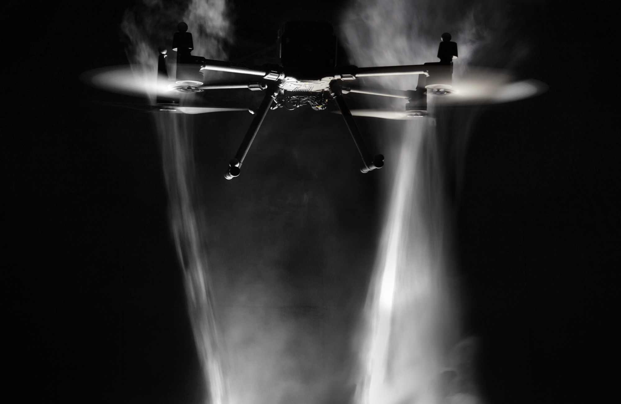
Figure 1: A smoke visualization of the near-field flow at hover where the flow contributions of the individual propellers are separated. Further downstream they merge into one turbulent jet (far-field).

Detailed computation of the induced flow around a drone is a very challenging problem as it requires expensive and time-consuming simulations involving computational fluid dynamics (CFD). To limit the computational demand, CFD simulations typically focus on a very short time-scale and are limited to only simulate the airflow close to the vehicle [18, 19, 20]. This methodology is suitable to assess the performance of the drone, but not suited to analyze the far-field which extends over many meters away from the drone where one needs to rely on turbulence modeling [15, 17]. Additionally, a CFD-based approach is not suitable for a real-time planner to dynamically coordinate a fleet of multiple quadrotors, such that the vehicles minimize interference with each other.

Orthogonal to the simulation approach, fluid dynamics research has a century-old history of heavily relying on empirical measurement. However, experimentally characterizing each drone with thousands of measurements in the entire 3D space around it is a tedious process. Firstly, performing experiments requires a wind-free (indoor) measurement domain much larger than the drone itself to properly identify the aerodynamic signature downstream. Secondly, a proper measurement technique needs to be selected. For example Particle Image Velocimetry (PIV) [21] is well suited, but generally presents additional challenges in large-scale real-world deployments [22, 23].

Contribution

In this paper, we present a unified, computationally lightweight model to calculate the mean velocity field of the induced flow around a drone at hover. The unified model is inspired by decades of well-established research on turbulent jets [24]. The advance in this work is enabled by joining methodologies from fluid dynamics and robotics research. Recording over 9 h of manual and autonomous drone flight data with three differently sized drones ranging from 572 g to 6.3 kg we perform pointwise flow measurements in a very large motion capture system [25] to acquire thousands of data samples of the mean velocity magnitude. Through the use of appropriate normalization and the introduction of a characteristic length, the model is unified and can be applied to quadrotors of different mass and size.

Our methodology is computationally lightweight as it does not rely on CFD simulations. Instead, it uses available closed-form analytic flow solutions. All calculations only require knowledge of the vehicle’s mass, the vehicle’s dimensions, and the propeller size.

II Related Work

For control and simulation tasks the primary goal of a model is to predict the motion of the vehicle given a certain actuation, that is, predict the forces and torques acting on the vehicle. The most widespread models are quadratic thrust and drag models [26, 27, 28] and more advanced models are based on blade-element-momentum (BEM) theory which calculates the lift and drag a propeller based on classical theory for airfoils [29, 30, 31, 32, 33, 34, 35]. However, these approaches only estimate the aerodynamic forces and torques of the propeller and do not compute the volumetric flow induced by the vehicle.

In contrast to the above models, computational fluid dynamics simulations calculate the three-dimensional flow around the vehicle. Such approaches are typically used to determine and improve the efficiency of the design of a single propeller [36, 37], but have also been applied to simulate entire quadrotors [20, 19], and larger hexacopters [38, 15]. While such simulations achieve results that are highly accurate and manage to capture real-world effects well [39, 40], they require large amounts of computation. Additionally, they do not generalize to other vehicles, requiring a new analysis for every drone.

In contrast to a purely simulation-based approach, a few works perform real-world experiments. For example, [13] performed flow probe measurements on a hexacopter that seem to find overall agreement with later CFD work [15]. In [41] the authors present experimental data to understand the influence of the quadrotor on atmospheric temperature and pressure measurements. In [42] the authors focus on the development of a Schlieren-photography method to qualitatively visualize the flow around drones. In [14] the authors performed outdoor smoke visualization, and in [43] the authors applied PIV to smoke visualizations to estimate the velocity field around a quadrotor model in ground effect. Only a few other studies have applied PIV to drones. For example, in [44] the interaction between propellers under different configurations has been studied, and in [45] the near field flow of a quadrotor model in forward flight is analyzed using wind tunnel experiments. Most recently  [11] performed PIV in a different application and recovered the spreading rate of spray droplets in the drone’s downwash.

Apart from [14, 41], all of these works performed measurements in tethered flight, presenting actual limitations in recovering the true free flight physics. To the authors’ best knowledge, no studies have looked into a comprehensive analysis of the flow around drones in hover while focusing on a scaling analysis, and on closed-form solutions from turbulent flows.

III Theory

This section gives an overview of the relevant notation, overall drone thrust and propeller downwash in hovering flight, and introduces the concept of a free jet. Finally, we introduce several normalizations enabling the analysis to generalize across a wide variety of drones.

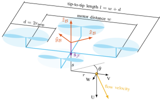
Figure 2: Diagram for the drone and the flow coordinate system and geometry. The bodyframe $\mathcal{B}$ of a quadrotor is such that the x-axis faces forward, and the z-axis upwards in thrust direction. The flow coordinate system is oriented such that its longitudinal axis $\mathbf{\hat{s}_{\mathcal{F}}}$ is aligned with flow direction (i.e., points in negative $\mathbf{\hat{z}_{\mathcal{B}}}$ direction). The flow is described in cylindrical coordinates $[s~{}~{}r~{}~{}\theta]^{\top}$ by its longitudinal (axial), radial, and azitmutal velocity components $U$, $V$ and $W$, respectively. The vehicle’s propeller diameter $d$, motor-distance $w$ and tip-to-tip length $l$ are defined as depicted.

III-A Coordinate System and Notation

Figure 2 shows the quadrotor-centered bodyframe coordinate system $\mathcal{B}$, with vector $\mathbf{x}_{\mathcal{B}}=[x~{}~{}y~{}~{}z]^{\top}$. In the bodyframe the $\mathbf{\hat{x}_{\mathcal{B}}}$-axis points forward, the $\mathbf{\hat{y}_{\mathcal{B}}}$-axis points to the left, and the $\mathbf{\hat{z}_{\mathcal{B}}}$-axis points upwards. Since we only consider the quadrotor at hover, the $\mathbf{\hat{z}_{\mathcal{B}}}$-axis is opposing the gravity vector at all times and no rotation due to the roll and pitch of the vehicle need be considered. We also introduce a flow coordinate system $\mathcal{F}$ with $\mathbf{x}_{\mathcal{F}}=[s~{}~{}r~{}~{}\theta]^{\top}$ in cylindrical coordinates along the flow direction $\mathbf{\hat{s}_{\mathcal{F}}}$. The longitudinal coordinate $s$ is aligned along the downwash direction and the radial coordinate $r$ points outwards as shown in Fig. 2. In this coordinate system the velocity vector $\mathbf{U}$ with components $U,V,W$ is defined as shown in Fig. 2.

III-B Propeller-Induced Flow

In a steady-state hover, the multicopter must produce enough thrust to support its weight. This means that—considering a quadrotor—the $N_{r}=4$ propellers must produce a thrust force that is equal to $mg$ where $m$ is the mass and $g$ is the gravitational acceleration.

A propeller produces lift force by accelerating air downwards. Assuming that the air above the propeller is at rest and that the air is accelerated in a virtual flow tube around the propeller a momentum balance across the propeller yields the induced-velocity $U_{\rm{H}}$ at hover [29]:

$$U_{\rm{H}}=\sqrt{\frac{T_{\rm{H}}}{2\rho A_{\text{prop}}}}=\sqrt{\frac{\vphantom{T}mg}{2\rho\pi r_{\text{prop}}^{2}N_{r}}}\ ,$$ (1)

where $T_{\rm{H}}$ is the hover thrust and $\rho$ is the air density. For the definition above, we assume that the flow tube has the same width as the propeller diameter, e.g. the induced velocity is calculated directly below the propeller. This model is an oversimplification and, for example, does not capture the true velocity profile of the flow below the propeller. However, as the model represents an overall momentum balance it can be interpreted as an average velocity across the flow tube close to the propeller [29, 46, 30].

III-C Turbulent Jet Flow

The key idea of our simple quadrotor aerodynamic model is to approximate the combined rotor-induced flow as a turbulent jet [24]. Because the airflow is turbulent, we do not consider the instantaneous flow values, instead we focus on time-averaged flow variables denoted by the averaging brackets $\langle\cdot\rangle$. For a turbulent jet, the mean longitudinal flow velocity $\langle U\rangle$ along the radial and flow-direction coordinates $r,s$ is given by the similarity profile [24]:

$$\langle U\rangle(\xi)=\frac{U_{\text{C}}(s)}{\left(1+\left(\sqrt{2}-1\right)\xi^{2}\right)^{2}}\;.$$ (2)

Here $U_{\text{C}}$ describes the centerline velocity at $r=0$ as function of the distance $s$ below the rotor plane. For a jet with half-width $r_{1/2}$, the rescaled radial position $\xi$ is given by:

$$\xi=\frac{r}{r_{1/2}(s)}\ .$$ (3)

The jet centerline velocity scales inversely proportional to the distance to the rotor plane. It can be calculated as

$$U_{\text{C}}(s)=U_{\text{J}}\frac{B\,d}{s-s_{0}}\ ,$$ (4)

where $U_{\text{J}}$ is initial jet velocity, $d$ the jet exit diameter, $B$ an empirical constant, and $s_{0}$ is the flow development-length. In addition, the jet half-width spreads linearly as

$$r_{1/2}(s)=S(s-s_{0})\ ,$$ (5)

where $S$ is the spreading rate that relates to the jet opening angle $\theta=2\arctan{(S)}$.

A key characteristic of the turbulent jet is that the spreading angle is commonly around 12 deg and is weakly dependent on the flow Reynolds number [24], making the model applicable to a wide range of drone flow and geometry. Furthermore, we remark that we do not need to consider propeller swirl in the analysis as the rotors counter-rotate, and we assume that all other flow components are entrained (drawn/sucked into the flow from the side) downstream.

III-D Normalization

To develop a generalized model of the airflow around different drones, the different phyiscal properties of those drones must be taken into account. We achieve this through introducing a velocity and a spatial normalization based on the theoretical considerations described previously.

Velocity Normalization

From (2) and (4) we observe that the overall scaling of the jet velocity is given by the jet-exit velocity $U_{\text{J}}$. The jet exit velocity is a quantity that describes how fast a turbulent jet exits the nozzle and captures how much momentum the flow carries. While a quadrotor does not have a nozzle, the induced velocity $U_{\rm{H}}$ of eq. (1) relates to the same physical quantity. Denoting a normalized quantity with $\sim$, the normalized velocity $\tilde{U}$ and normalized centerline velocity $\tilde{U}_{C}$ are given by:

$$\langle\tilde{U}\rangle(\xi)=\frac{\langle U\rangle(\xi)}{U_{\rm{H}}}\quad\text{and}\quad\tilde{U}_{\text{C}}(s)=\frac{U_{\text{C}}(s)}{U_{\rm{H}}}\;.$$ (6)

Length-Scale Normalization

Similar to the velocity normalization, a spatial normalization parameter is needed to be able to compare drones of different sizes. We propose the tip-to-tip length $l$ as the length-scale parameter as this distance is closest equivalent to the nozzle diameter in a jet flow. Using this, we define the normalized distance to the rotor plane $\tilde{s}$, the normalized radial distance $\tilde{r}$ and the normalized half-width $\tilde{r}_{1/2}$ as:

$$\tilde{s}=\frac{s}{l},\quad\tilde{r}=\frac{r}{l},\quad\text{and}\quad\tilde{r}_{1/2}(s)=\frac{r_{1/2}(s)}{l}\;.$$ (7)

IV Flight Experiments

IV-A Experimental Setup

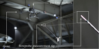
Figure 3: The DJI Matrice 300 drone hovers in proximity of the flow probe. The inset shows a close-up view of the Testo hotball probe. The flow probe measures the speed of the airflow.

Measurements of the flow around a drone require a large indoor space to avoid a recirculation of air while preventing external disturbances such as wind. A key enabler of this study is the access to a large industrial hall equipped with a 36-camera Vicon motion-capture system covering a tracking volume of $25\times 25\times 7\,\mathrm{m}$. This motion-capture system enables recording the position of the drone with millimeter accuracy.

The flow is measured with an omnidirectional hotball flowprobe (Testo 440). This type of commercial, off-the-shelf anemometer is indifferent to the flow direction and presents a sufficiently high measurement accuracy of $\pm 0.03\,\mathrm{m/s}\pm 5\%$ (up to 20 m/s) at a sampling rate of 1 s. This is favorable as we are interested in the induced mean magnitude and not the fluctuating velocity components of vortices in the turbulent flow. As shown in Fig. 3, the flow probe is mounted on a long pole at a height of 4.5 m, roughly corresponding to a normalized height of 5 tip-to-tip lengths of the drone.

IV-B Quadrotors

For experiments three different quadrotors are used whose properties are summarized in Tab. I. The vehicles Offboard 1 and Offboard 2 are research drones that can autonomously fly missions [47] and are controlled through the motion-capture system. Both drones share the same frame, however drone 2 has double the mass compared to drone 1. We also use a DJI Matrice 300 drone as a much larger and heavier vehicle. This allows us to demonstrate the generality of the proposed jet flow model and underlying theoretic framework. In contrast to the research drones, the commercial DJI drone in this study must be flown manually throughout the entire experiment.

TABLE I: Overview of the quadrotors.

	Mass	Propeller Diameter	Motor Distance	Induced Velocity
Offboard 1	0.572 kg	12.95 cm	26.6 cm	6.66 m/s
Offboard 2	1.207 kg	12.95 cm	26.6 cm	9.66 m/s
Matrice 300	6.300 kg	53.34 cm	89.4 cm	5.36 m/s

IV-C Data Collection

To collect the experimental data, each vehicle is flown in a grid-like pattern where the drone approaches a point, steadily hovers for 5 s to allow the flow to (re-)develop and then slowly translates to the next point in the three-dimensional flight path. For the autonomous drones we sample a coarse grid spanning $3\times 3\times 2.5\,\mathrm{m}$ with a spacing of 15 cm in the $xy$-plane and 50 cm in $z$ and a fine grid spanning $0.5\times 0.5\times 2.5\,\mathrm{m}$ with a resolution of 10 cm in the $xy$-plane and 30 cm in $z$. For the Matrice 300 the pilot covered a much larger area of $5\times 6\times 4.5\,\mathrm{m}$.

Transforming the flight data into the drones’ reference frame, we filter out all data points where the vehicle moves with more than 0.1 m/s speed during the sampling interval. This reduces the influence of transient effects and ensures high data quality. Despite being in a large indoor space, the anemometer registers a small ambient flow in the range of 0.06 m/s to 0.12 m/s. As this is flow is already observed before the drone takes off, it is not primarily caused by recirculation effects but related to the testing facility. The background level is about 2 orders of magnitudes below the induced velocities. We correct for the static offset by subtracting the ambient airflow speed from the measurements.

After filtering we obtain 12000 s of flight data for each of the three vehicles. The raw measurement data is in the form of a position measurement and a corresponding anemometer measurement. For further processing, this scattered data is converted into binned gridded data by combining all measurements within a grid cell. To increase the robustness of the measurements, the median value of the cell is used and the empirical standard deviation is calculated.

V Results: Near Field

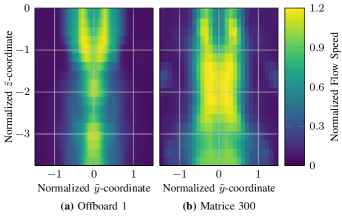
Figure 4: Visualization of the near field of (a) the Offboard 1 drone and (b) the Matrice 300. The length and velocity scales are normalized. The influence of the individual propellers is clearly visible at $z=0$ and diminishes at a normalized distance of about 2.

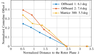
Figure 5: The plot shows the distance $\tilde{\delta}$ of the flow tube centerline to the $\mathbf{z}_{\mathcal{B}}$ axis. Very close to the rotor-plane of the vehicle (left side of the plot) the flow has not fully developed. From between two and three length scales below the drone the flow has fully developed with the highest velocity being measured on the negative z-axis of the drone.

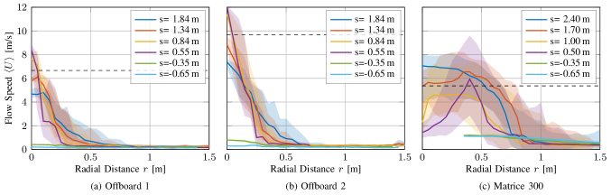
Figure 6: Radial velocity profiles for the three different drones. The colors show different height levels. The shaded area indicates the $1\sigma$ uncertainty region around the mean, the line shows the median value. The dashed line shows the induced velocity at hover.

In a first analysis we focus on the flow directly below the drone in the region where the flow contributions of the four individual propellers are seperated and not yet have fully merged into one turbulent jet. The goal is to analyse how the flow from the individual propellers merge into a combined turbulent jet for the different quadrotors.

Figure 4 visualizes the flow field for a $yz_{\mathcal{B}}$-slice from the measurement data. The quadrotor is located at the ‘top’ of the plot (e.g. at $\tilde{z}$=0) and one can clearly see the two separate jets induced by the left and the right propellers. The Offboard 1 and Matrice 300 drone show similar flow patterns as we normalize the axes with the drones’ tip-to-tip dimensions. This indicates that the tip-to-tip length is an appropriate scaling for the drones’ flow geometry.

In between the two jets, a region of reduced flow speed can be observed. This depression is due to the separation of the drones’ rotors and the blocking of the flow by its main body. Such flow structures have previously been observed in CFD simulations [14] and validation studies [13], and are consistent with our results. Afterward, the jets start to converge at about one length scale below the rotor plane. From about two length scales below the drone, the jets appear to have fully merged. In metric coordinates this corresponds to about 0.5 m below the Offboard 1 drone and 2 m below the Matrice 300.

Figure 5 quantitatively describes the merging of the individual jets. The distance of the maximum propeller flow velocity centerline to the drones’ negative $\mathbf{z}_{\mathcal{B}}$ axis is considered. This distance is estimated by first extracting the $\tilde{y}$-axis velocity profile for different distances below the drone. Then this empirical profile is approximated with a $z_{\mathcal{B}}$-axis symmetric bimodal Gaussian where the means are shifted $\pm\tilde{\delta}$ along the $\tilde{y}$-axis. In agreement with related works [14] we find that for all drones in this study, the individual rotor flows merge between 2 and 2.5 tip-to-tip dimensions below the drone.

VI Results: Far Field

From the preliminary considerations of the airflow close to the vehicle, we see that the individual contributions from the quadrotor’s four propellers merge together about two length scales below the drone. In this section, we present our novel experimental findings to answer the question:‘How much wind do the quadrotors make away from their propellers in the far field?’.

For the remainder of this section, cylindrical coordinates are used. The data is binned radially along $r$ and analyzed for downstream coordinates $s$, following the convention introduced in Fig. 2.

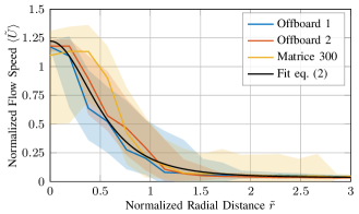
Figure 7: Radial velocity profiles for the three drones at a normalized height of $\tilde{s}=-3.0$. The shaded area indicates the $1\sigma$ uncertainty region around the mean, the line shows the median value. The proposed normalization leads to all curves being similar within measurement accuracy. The black line represents the radial velocity profile for a turbulent jet eq. (2).

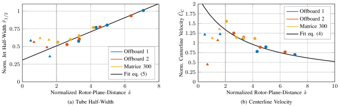
Figure 8: Downstream scaling parameters of the flow. Only datapoints in the far field region (marked with a circle) are used to fit the function predicted by turbulet jet theory. (a) The plot depicts the (normalized) tube half-width $\tilde{r}_{1/2}$ as a function of the (normalized) distance to the rotor plane $\tilde{s}$. We recover the characteristic spreading angle for turbulent jets of 12 deg. (b) The plot focuses on the (normalized) centerline velocity $\tilde{U}_{\text{C}}$ as a function of the (normalized) distance to the rotor plane. We recover the characteristic $1/(s-s_{0})$ scaling from eq. (4).

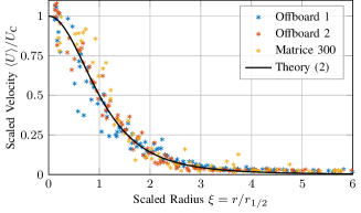
Figure 9: Unified formulation of the flow. The measurement samples from all drones across the entire far field show good agreement with turbulent jet theory eq. (2) (black line).

VI-A Radial Velocity Profiles

Figure 6 shows radial profiles of the mean velocity for the three drones at different heights. First, for all drones, the peak measured velocities exceed the calculated induced velocity at hover by 25 % at maximum. This small mismatch with the calculated propeller induced flow is expected as the velocity profile in the merged flow is not constant across the cross section and by conservation of momentum the peak velocity is higher. Second, we compare measurements at different $s$-coordinates for each drone and observe that the mean flow velocities all decay radially from the drone. Third, the downstream peak velocity rapidly decreases away from the drone, while the flow domain spreads out. Finally, comparing measurements above and below the drone, we see that the flow velocity above the drone ($s=-0.35\,\mathrm{m}$ and $s=-0.65\,\mathrm{m}$) is much lower compared to below the drone as the flow is uniformly sucked into the propellers from all directions.

We now look at the same data using the normalization introduced in Sec. III-D. The plot in Fig. 7 corresponds to a normalized $\tilde{s}$ level at 3 length scales (e.g. tip-to-tip distance) below the drone. The normalized, time-averaged measured velocity $\langle\tilde{U}\rangle$ is plotted as a function of the normalized radial coordinate $\tilde{r}$ and each color now corresponds to one drone. We can clearly see that, within the given measurement accuracy, the curves overlap which empirically validates the proposed normalization as it makes the airflow around different vehicles similar. Additionally, the radial velocity profile across all drones is well captured fitting eq.(2), inset in black in Fig. 7. This provides the first evidence that the combined rotor flow can be treated as a turbulent jet.

VI-B Jet Flow Scaling

Next, we focus on the expansion of a turbulent jet which is described by eq. (5). For a turbulent jet, the flow expands linearly as a cone with approximately 12 deg opening angle [24] over a wide range of flow Reynolds number. Furthermore, the jet’s centerline velocity scales inversely proportional with the distance to the nozzle as described by eq. (4).

In Figure 8 we find very good agreement with these two characteristics for the combined rotor flow of a quadrotor after $\tilde{s}=2$. Figure 8a and b show the normalized half-width $\tilde{r}_{1/2}$ and the normalized centerline velocity $\langle\tilde{U}_{\text{C}}\rangle$ of the radial velocity profiles as a function of the normalized distance $\tilde{s}$ to the drone’s rotor plane. The half-width and velocity have been obtained by fitting the velocity profile eq. (2) to the measurements at each $\tilde{s}$-slice for each drone. The triangles indicate datapoints located in the near-field (not considered for the fit) and circles indicate measurements from the far field (considered for the fit). The black lines represent a fit using the function form prescribed by the turbulent jet model eq. (5) and (4). The parameters obtained from the fit are

$$B\,d=6.84\,,\quad S=0.0997\,\text{~{}and}\quad s_{0}=3.08\;.$$ (8)

The scaling parameters (8) can be used to fully describe the turbulent jet flow in eq. (2). This velocity profile from eq. (2) is shown with the black line in Fig. 9 and is not fitted to the data. The measurement samples are taken from all drones across the entire far field and measurement scaling is computed using eq. (5) and (4) with the parameters above. The good agreement with the theory shows that the measured velocity of a quadrotor field in both axial and radial dimension is well captured by the theory of turbulent jets.

VI-C Unified Model

To use the unified model describing the far field flow of a quadrotor, we combine the results demonstrating normalization and scaling. As demonstrated in Fig. 7, the normalization of the drones’ propeller-induced flow and geometry of Sec. III-D makes drones of different mass and size similar. The recovered scaling parameters for eq. (5) and (4) enable us to leverage self-similarity to fully describe the downwash of the quadrotor as a turbulent jet (see Fig. 9).

To calculate the time-averaged velocity $\langle U\rangle$ in the far field below a quadrotor at a point $\mathbf{p}=[s~{}~{}r~{}~{}\theta]^{\top}$, perform the following operations:

1. Normalization parameter: Use the physical parameters (mass, propeller size, number of propellers) of the quadrotor to calculate the induced velocity at hover $U_{\rm{H}}$ using eq. (1) and the tip-to-tip length $l$ .

2. Normalize the point’s length-scale: $\tilde{s}=s/l$, $\tilde{r}=r/l$.

3. Calculate the normalized turbulent jet scaling $\tilde{r}_{1/2}$ and $\tilde{U}_{\text{C}}$ for the normalized point. This is done with eq. (4) (set $U_{\text{J}}=1$) and (5) together with the parameters (8).

4. Calculate the scaled radial position $\xi=\tilde{r}/\tilde{r}_{1/2}$.

5. Scale the centerline velocity $U_{\text{C}}=\tilde{U}_{\text{C}}\cdot U_{\rm{H}}$.

6. Finally, use $\xi$ and $U_{\text{C}}$ to evaluate the time-averaged flow speed using the turbulent jet equation (2).

Note that, in case of interest, the entrained radial mean flow component $\langle V\rangle$ can be obtained through continuity [24].

VII Conclusion and Discussion

This work presents a model for the far field flow of a drone, based on classical turbulent jet theory. We have recorded a large-scale dataset comprising three drones and containing over 9 h of flight data in a motion-capture system while measuring the airflow with a hot-ball flow probe. Leveraging normalization techniques relying on the physical parameters of the vehicle (mass, propeller size, vehicle size), the airflow of different sizes of drones is comparable.

We study the flow in the near-field flow close to the drone and find that the individual flows from the propellers merge approximately two tip-to-tip length scales below the drone. In this near-flow region, the interactions between the flow and the drone are dominant which can only be fully captured through CFD simulations. However, when considering the effects of the induced flow on the environment and other agents, the primary concern is the far-field extending from about two length scales downwards.

Through the use of a scaling approach from turbulent jet theory, we develop a unified model that describes the far field flow below the drone. The experiments show that, despite the simplicity of the model, it is able to accurately describe the flow. This makes our model ideally suited for integration in a dynamic planner and in multi-agent scenarios. We believe that this is an important step towards safer and less intrusive drones, an aspect becoming increasingly important with the increasing adoption of quadrotors. Understanding the flow also enables optimized sensor placement for scientific applications and potentially higher efficiency when quadrotors are deployed in an agricultural context.

References

- [1] E. Kaufmann, L. Bauersfeld, A. Loquercio, M. Müller, V. Koltun, and D. Scaramuzza, “Champion-level drone racing using deep reinforcement learning,” Nature, vol. 620, no. 7976, pp. 982–987, Aug 2023.
- [2] R. D’Andrea, “Guest editorial: Can drones deliver?” IEEE Transactions on Automation Science and Engineering, 2014.
- [3] K. Karydis and V. Kumar, “Energetics in robotic flight at small scales,” Interface Focus, 2017.
- [4] K. Mohta, M. Watterson, Y. Mulgaonkar, S. Liu, C. Qu, A. Makineni, K. Saulnier, K. Sun, A. Zhu, J. Delmerico, K. Karydis, N. Atanasov, G. Loianno, D. Scaramuzza, K. Daniilidis, C. J. Taylor, and V. Kumar, “Fast, autonomous flight in gps-denied and cluttered environments,” Journal of Field Robotics, 2018.
- [5] “DJI Camera Drones,” https://www.dji.com/camera-drones, accessed: 2024-02-25.
- [6] “Flyability Elios-3,” https://www.flyability.com/elios-3, accessed: 2024-02-25.
- [7] “Skydio X10 Drone,” https://www.skydio.com/x10, accessed: 2024-02-25.
- [8] “Parrot Drones,” https://www.parrot.com/us, accessed: 2024-02-25.
- [9] C. E. Comission, “Aerialcore,” https://aerial-core.eu/, accessed: 2024-03-13.
- [10] ——, “Autoassess,” https://autoassess.eu/, accessed: 2024-03-13.
- [11] K. Chang, S. Chen, M. Wang, X. Xue, and Y. Lan, “Numerical simulation and verification of rotor downwash flow field of plant protection uav at different rotor speeds,” Frontiers in Plant Science, vol. 13, 2023.
- [12] N. Simon, A. Z. Ren, A. Piqué, D. Snyder, D. Barretto, M. Hultmark, and A. Majumdar, “Flowdrone: Wind estimation and gust rejection on uavs using fast-response hot-wire flow sensors,” in 2023 IEEE International Conference on Robotics and Automation (ICRA). IEEE, May 2023.
- [13] T. F. Villa, F. Salimi, K. Morton, L. Morawska, and F. Gonzalez, “Development and validation of a uav based system for air pollution measurements,” Sensors, vol. 16, no. 12, 2016.
- [14] C. Crazzolara, M. Ebner, A. Platis, T. Miranda, J. Bange, and A. Junginger, “A new multicopter-based unmanned aerial system for pollen and spores collection in the atmospheric boundary layer,” Atmospheric Measurement Techniques, vol. 12, no. 3, pp. 1581–1598, 2019.
- [15] K. A. McKinney, D. Wang, J. Ye, J.-B. de Fouchier, P. C. Guimarães, C. E. Batista, R. A. F. Souza, E. G. Alves, D. Gu, A. B. Guenther, and S. T. Martin, “A sampler for atmospheric volatile organic compounds by copter unmanned aerial vehicles,” Atmospheric Measurement Techniques, vol. 12, no. 6, pp. 3123–3135, June 2019.
- [16] W. Thielicke, W. Hübert, U. Müller, M. Eggert, and P. Wilhelm, “Towards accurate and practical drone-based wind measurements with an ultrasonic anemometer,” Atmospheric Measurement Techniques, vol. 14, no. 2, pp. 1303–1318, 2021.
- [17] M. Ghirardelli, S. T. Kral, N. C. Müller, R. Hann, E. Cheynet, and J. Reuder, “Flow structure around a multicopter drone: A computational fluid dynamics analysis for sensor placement considerations,” Drones, vol. 7, no. 7, 2023.
- [18] C. Paz, E. Suárez, C. Gil, and J. Vence, “Assessment of the methodology for the cfd simulation of the flight of a quadcopter uav,” Journal of Wind Engineering and Industrial Aerodynamics, vol. 218, p. 104776, 2021.
- [19] P. Ventura Diaz and S. Yoon, “High-fidelity computational aerodynamics of multi-rotor unmanned aerial vehicles,” in 2018 AIAA Aerospace Sciences Meeting, 2018, p. 1266.
- [20] J. Luo, L. Zhu, and G. Yan, “Novel quadrotor forward-flight model based on wake interference,” Aiaa Journal, vol. 53, no. 12, pp. 3522–3533, 2015.
- [21] R. Adrian and J. Westerweel, Particle Image Velocimetry. Cambridge: Cambridge University Press, 2011.
- [22] M. Kühn, K. Ehrenfried, J. Bosbach, and C. Wagner, “Large-scale tomographic particle image velocimetry using helium-filled soap bubbles,” Experiments in Fluids, vol. 50, no. 4, pp. 929–948, August 2010.
- [23] C. Jux, A. Sciacchitano, J. F. G. Schneiders, and F. Scarano, “Robotic volumetric piv of a full-scale cyclist,” Experiments in Fluids, vol. 59, no. 4, p. 74, Apr 2018.
- [24] S. B. Pope, Turbulent Flows. Cambridge University Press, 2000.
- [25] A. Mueller, A. Landolt, and T. K. Rösgen, Probe capture for quantitative flow visualization in large scale wind tunnels.
- [26] R. Mahony, V. Kumar, and P. Corke, “Multirotor aerial vehicles: Modeling, estimation, and control of quadrotor,” IEEE Robotics and Automation magazine, vol. 19, no. 3, pp. 20–32, 2012.
- [27] F. Furrer, M. Burri, M. Achtelik, and R. Siegwart, “Rotors—a modular gazebo mav simulator framework,” in Robot Operating System (ROS). Springer, 2016, pp. 595–625.
- [28] S. Shah, D. Dey, C. Lovett, and A. Kapoor, “Airsim: High-fidelity visual and physical simulation for autonomous vehicles,” in Field and service robotics. Springer, 2018, pp. 621–635.
- [29] R. W. Prouty, Helicopter performance, stability, and control, 1995.
- [30] L. Bauersfeld, E. Kaufmann, P. Foehn, S. Sun, and D. Scaramuzza, “Neurobem: Hybrid aerodynamic quadrotor model,” RSS: Robotics, Science, and Systems, 2021.
- [31] W. Khan and M. Nahon, “Toward an accurate physics-based uav thruster model,” IEEE/ASME Transactions on Mechatronics, vol. 18, no. 4, pp. 1269–1279, 2013.
- [32] R. Gill and R. D’Andrea, “Propeller thrust and drag in forward flight,” in 2017 IEEE Conference on Control Technology and Applications (CCTA). IEEE, 2017, pp. 73–79.
- [33] R. Gill and R. D’Andrea, “Computationally efficient force and moment models for propellers in uav forward flight applications,” Drones, vol. 3, no. 4, p. 77, 2019.
- [34] G. Hoffmann, H. Huang, S. Waslander, and C. Tomlin, “Quadrotor helicopter flight dynamics and control: Theory and experiment,” in AIAA guidance, navigation and control conference and exhibit, 2007, p. 6461.
- [35] H. Huang, G. M. Hoffmann, S. L. Waslander, and C. J. Tomlin, “Aerodynamics and control of autonomous quadrotor helicopters in aggressive maneuvering,” in 2009 IEEE international conference on robotics and automation. IEEE, 2009, pp. 3277–3282.
- [36] D. Ragni, B. Van Oudheusden, and F. Scarano, “Non-intrusive aerodynamic loads analysis of an aircraft propeller blade,” Experiments in fluids, vol. 51, no. 2, pp. 361–371, 2011.
- [37] W. Westmoreland, R. Tramel, and J. Barber, “Modeling propeller flow-fields using cfd,” in 46th AIAA Aerospace Sciences Meeting and Exhibit, 2008, p. 402.
- [38] Y. ZHENG, S. YANG, X. LIU, J. WANG, T. NORTON, J. CHEN, and Y. TAN, “The computational fluid dynamic modeling of downwash flow field for a six-rotor uav,” Frontiers of Agricultural Science and Engineering, vol. 5, no. 2, p. 159, 2018.
- [39] H. Yasuda, K. Kitamura, and Y. Nakamura, “Numerical analysis of flow field and aerodynamic characteristics of a quadrotor,” Transactions of The Japan Society for Aeronautical and Space Sciences, Space Technology Japan, vol. 11, pp. 61–70, 2013.
- [40] S. Yoon, Nasa, P. V. Diaz, D. D. J. Boyd, W. M. Chan, and C. R. Theodore, “Computational aerodynamic modeling of small quadcopter vehicles,” 2017.
- [41] F. Pätzold, A. Bauknecht, A. Schlerf, D. Sotomayor Zakharov, L. Bretschneider, and A. Lampert, “Flight experiments and numerical simulations for investigating multicopter flow field and structure deformation,” Atmosphere, vol. 14, no. 9, 2023.
- [42] X. Liu, T. Guo, P. Zhang, Z. Jia, and X. Tong, “Extraction of a weak flow field for a multi-rotor unmanned aerial vehicle (uav) using high-speed background-oriented schlieren (bos) technology,” Sensors, vol. 22, no. 1, 2022.
- [43] H. Otsuka, M. Kohno, and K. Nagatani, “Flow visualization of wake of a quad-copter in ground effect,” in 6th Asian-Australian Rotorcraft Forum and Heli Japan 2017, ARF 2017, 2017.
- [44] D. Shukla and N. Komerath, “Multirotor drone aerodynamic interaction investigation,” Drones, vol. 2, no. 4, 2018.
- [45] Z. Czyż, P. Karpiński, and W. Stryczniewicz, “Measurement of the flow field generated by multicopter propellers,” Sensors, vol. 20, no. 19, 2020.
- [46] G. Hoffmann, H. Huang, S. Waslander, and C. Tomlin, “Quadrotor helicopter flight dynamics and control: Theory and experiment,” in AIAA guidance, navigation and control conf., 2007.
- [47] P. Foehn, E. Kaufmann, A. Romero, R. Penicka, S. Sun, L. Bauersfeld, T. Laengle, G. Cioffi, Y. Song, A. Loquercio, and D. Scaramuzza, “Agilicious: Open-source and open-hardware agile quadrotor for vision-based flight,” Science Robotics, vol. 7, no. 67, 2022.