Kernel Multigrid: Accelerate Back-fitting via Sparse Gaussian Process Regression
Abstract
Additive Gaussian Processes (GPs) are popular approaches for nonparametric feature selection. The common training method for these models is Bayesian Back-fitting. However, the convergence rate of Back-fitting in training additive GPs is still an open problem. By utilizing a technique called Kernel Packets (KP), we prove that the convergence rate of Back-fitting is no faster than , where and denote the data size and the iteration number, respectively. Consequently, Back-fitting requires a minimum of iterations to achieve convergence. Based on KPs, we further propose an algorithm called Kernel Multigrid (KMG). This algorithm enhances Back-fitting by incorporating a sparse Gaussian Process Regression (GPR) to process the residuals after each Back-fitting iteration. It is applicable to additive GPs with both structured and scattered data. Theoretically, we prove that KMG reduces the required iterations to while preserving the time and space complexities at and per iteration, respectively. Numerically, by employing a sparse GPR with merely 10 inducing points, KMG can produce accurate approximations of high-dimensional targets within 5 iterations.
Keywords: Additive Gaussian Processes; Back-fitting; Kernel Packet; Convergence Rate.
1 Introduction
Additive Gaussian Processes (GPs) are popular approaches for nonparametric feature selection, effectively addressing high-dimensional generalized additive models (Hastie, 2017) from a Bayesian perspective. This method posits that the high-dimensional observed data can be decomposed into an additive form of one-dimensional GPs, expressed as . It then leverages Bayes’ rule to infer the posterior distribution of the contributions from each dimension individually. Thus, additive GPs offer not only high interpretability but also uncertainty quantification of their outcomes by providing distributions for the posteriors.
Despite their considerable benefits, additive GPs come with significant drawbacks, in brief their computational complexity. Training an additive GP model necessitates performing matrix multiplications and inversions. For training points in -dimension, matrix operations demand time and space. These complexities can be prohibitive. Given that additive GPs are typically employed in high-dimensional problems with a substantial number of observations, direct computations become impractical. This computational burden severely limits the practicality of additive GPs in addressing many real-world problems.
Considerable research has been dedicated to enhancing the efficiency of computing the posteriors of additive GPs. Among these efforts, Bayesian Back-fitting (Breiman and Friedman, 1985; Hastie and Tibshirani, 2000; Saatçi, 2012) is one of the most commonly used algorithms for training additive GPs. Back-fitting, which allows a scalable fit over a single dimension of the input, can be used to fit an additive GP over a -dimensional space with the same overall asymptotic complexity. Specifically, Back-fitting iteratively conducts Gaussian Process Regression (GPR) for each dimension individually while holding the others fixed. Thanks to efficient algorithms for training one-dimensional GPR, such as the state-space model (Hartikainen and Särkkä, 2010) or kernel packets (KP) (Chen et al., 2022; Ding and Tuo, 2024), each Back-fitting iteration can be executed with efficient time and space complexities of and , respectively.
However, the convergence rate of Back-fitting for additive GPs remains an open problem. Despite its remarkable performance in prediction and classification tasks, as shown in (Gilboa et al., 2013; Delbridge et al., 2020), leading to speculation that Back-fitting may exhibit exponentially fast convergence for additive GPs, our analysis reveals a different picture. By employing a technique called Kernel Packet (KP), which provides an explicit formula for the inverse kernel matrix, we can prove that Back-fitting converges no faster than when focusing on convergence towards the posterior of each individual dimension. Here is the data size and is the iteration number. This finding implies that a minimum of iterations is necessary for Back-fitting to reach convergence. The intuition is that Back-fitting struggles to accurately distribute global features across the correct dimensions, although the composite structure of additive models for prediction or classification might compensate for errors resulting from such misallocations. Inspired by the Algebraic Multigrid method in numerical analysis, we introduce an algorithm named Kernel Multigrid (KMG). This approach refines Back-fitting by integrating a sparse GPR to handle residuals after each iteration. The inclusion of sparse GPR aids in efficiently reconstructing global features during each step of the iterative process, thereby effectively addressing the aforementioned limitation associated with Back-fitting. KMG is versatile, applicable to additive GPs across both structured and scattered data. If we impose a weak condition on the associated sparse GPR, we can prove that the algorithm significantly reduces the necessary iterations to while maintaining the time and space complexities unchanged for each iteration. Furthermore, through numerical experiments comparing Back-fitting and KMG, we find that with merely 10 inducing points in the sparse GPR, KMG is capable of accurately approximating high-dimensional targets in 5 iterations.
In summary, we have established a lower bound for the convergence rate of Back-fitting, demonstrating that a minimum of iterations is required for convergence. To address this limitation, we introduce the KMG algorithm, a slight modification of Back-fitting that overcomes its shortcomings. Consequently, KMG achieves exponential convergence towards each one-dimensional target posterior .
1.1 Literature Review
Scalable GPs aim to improve the scalability of full GP models without compromising the quality of predictions. Two prominent approaches in this domain are sparse approximation and iterative methods. Sparse approximation (Seeger et al., 2003; Snelson and Ghahramani, 2005; Quinonero-Candela and Rasmussen, 2005; Titsias, 2009; Eleftheriadis et al., 2023) rely on selecting a set of inducing points from a large pool of observation to effectively approximate the posterior at a time complexity of . The main challenge lies in optimally selecting inducing points to strike a balance between computational efficiency and prediction accuracy. Recently, several work including Wilson and Nickisch (2015); Hensman et al. (2018); Dutordoir et al. (2020); Burt et al. (2020) have attempted to investigate this issue. Typically, these approaches enable the utilization of a considerable number of inducing points with minimal cost; however, these methods require imposing certain restrictions to the subspaces used for approximation.
Iterative methods, particularly the Conjugate Gradients(CG) method (Lanczos, 1950; Hestenes et al., 1952; Saad, 2003), provide an alternative strategy for efficient approximation in GPs. Recently, there has been a notable increase in the popularity of iterative methods (Cutajar et al., 2016; Cockayne et al., 2019; Bartels and Hennig, 2020), largely due to their precision and effective utilization of GPU parallelization (Gardner et al., 2018). Numerous enhancements to CG method have been proposed to improve numerical stability and accelerate convergence speed. For example, Potapczynski et al. (2021) propose random truncations method to reduce the bias of CG. Similarly, Wenger et al. (2021) propose variance reduction techniques to reduce the bias of CG. Additionally, Maddox et al. (2021) provided comprehensive implementation guidance for the CG method, assisting practitioners in consistently attaining robust performance. For literature that delves into theoretical analysis of CG methods in GPs, please refer to (Wenger et al., 2022a, b). These iterative approaches have demonstrated effectiveness on large scale datasets (Wang et al., 2019). The performance of the CG is critically dependent on the initial solution and the preconditioner. An ill-chosen preconditioner can significantly impede convergence (Cutajar et al., 2016; Wu et al., 2023).
Multigrid methods (Saad, 2003; Borzi and Schulz, 2009) are classic computational techniques designed to solve partial differential equations (PDEs), serving as a complement to the CG methods in numerical computation. A key difference between Multigrid methods and the CG methods is that Multigrid methods cycle through various grid resolutions, transferring solutions and residuals between finer and coarser grids, whereas CG methods iteratively refines the solution by moving along conjugate directions. However, the application of Multigrid methods is constrained by their requirement for a grid-based domain and noiseless observations, which limits their suitability for GPR. Our method generalizes the idea of Multigrid methods for scatter datasets with noise.
Additive GP models (Duvenaud et al., 2011; Kaufman and Sain, 2010; López-Lopera et al., 2022; Lu et al., 2022) have recently attracted significant interest due to their broad applicability in various fields. The structure of additive GPs allows for implementation of Back-fitting. A key advantage of Back-fitting is its ability to update the posterior for each dimension at one time, thereby avoiding the costly joint updates (Luo et al., 2022). Furthermore, Back-fitting is also a popular methodology for training bayesian tree structure type model (Chipman et al., 2012; Linero, 2018; Lu and McCulloch, 2023), demonstrating its flexibility and effectiveness in various scenarios. Recently, the idea of projection pursuit Friedman and Stuetzle (1981) has been integrated into additive GPs, introducing greater flexibility and enhancing computational efficiency. For further reading on projection pursuit in additive GPs, please see Gilboa et al. (2013); Delbridge et al. (2020); Chen and Tuo (2022).
Back-fitting has also been extensively embraced in the context of additive models within the frequentist setting (Luo, 1998; Sadhanala and Tibshirani, 2019; El-Bachir and Davison, 2019). The consistency of the Back-fitting has been extensively studied in Buja et al. (1989); Ansley and Kohn (1994); Mammen et al. (1999). Recently, Ghosh et al. (2022a) developed a Back-fitting algorithm for generalized least squares estimators, demonstrating its operation at a complexity of under certain asymptotic conditions. This methodology has been extended to generalized linear mixed models for logistic regression (Ghosh et al., 2022b) and to generalized linear mixed models that include random slopes (Ghandwani et al., 2023). The existing literature on nonparametric additive models (Mammen and Park, 2006; Yu et al., 2008; Fan and Jiang, 2005; Opsomer, 2000) primarily focuses on the asymptotic properties of Back-fitting estimators, rather than its convergence rate. To the best of our knowledge, research on the convergence rate of Back-fitting for nonparametric additive models is scarce.
The paper is organized as follows. In Section 2 we provide an overview of the background knowledge for GPs, the KP technique, and Bayesian Back-fitting. In Section 3, we establish the lower bound of convergence for Bayesian Back-fitting. Section 4 introduces a novel algorithm named KMG, along with a discussion of its convergence properties. In Section 5, the performance of KMG is evaluated on both synthetic and real-world datasets. Finally, we conclude our findings and propose directions for future research in Section 6.
2 Preliminaries
GPs have emerged as a popular Bayesian method for nonparametric regression, offering the flexibility to establish prior distributions over continuous functions. In this section, we will introduce some foundational concepts in GPs relevant to our study.
2.1 General Gaussian Processes
A GP is a distribution on function over an input space such that the joint distribution of on any size- set of input points is described by a multivariate Gaussian density over the associated targets, i.e.,
where is an -vector whose -entry equals the value of a mean function on point and is an -by- kernel covariance matrix whose -entry equals the value of a positive definite kernel on and (Wendland, 2004). Accordingly, a GP can be characterized by the mean function and the kernel function . Generally , the mean function is set as when we have no prior knowledge of the true function. Therefore, we can use only the kernel to determine a GP.
In this study, we will assume that the underlying GP is stationary, i.e., its covariance only depends on the difference: . GPs with stationary kernels have been widely used in time series (see for example Brockwell and Davis (1991)) and spatial statistics (see for example Cressie (2015)). For a one-dimensional stationary , we can define its Fourier transform as follows:
Now we can impose the following specific assumption on the kernel function. This assumption is weak and includes a large number of kernel classes, such as the Matérn kernels and the compactly supported Wendland kernels (Wendland, 2004, Chapter 9).
Assumption 2.1
The kernel is stationary and its Fourier transform satisfies:
for some where and are positive constants independent of s, and kernel function k.
We consider the case that observation is noisy , where is an i.i.d. Gaussian distributed error. Then, we can use standard identities of the multivariate Gaussian distribution to show that, conditioned on data , the posterior distribution at any point also follows a Gaussian distribution: , where
| (1) |
where , and .
The computation of (1) all require time complexcity and space complexity due to the need for inverting dense matrices . When data size is large, GPs are computational inefficient and unstable because the kernel covariance matrix is dense and nearly singular.
2.2 Additive GPs
A -dimensional additive GP can be view as summation of one-dimensional GPs. Specifically,
where is a one-dimensional zero-mean GP characterized by kernel and is the -th entry of the -dimensional training point . So an additive GP has kernel function . We use the following model to describe the generation of observations :
| (2) |
An additive prior occupies a middle ground between a linear model, which is additive, and a nonlinear regression prior, allowing for the modeling of arbitrary interactions between inputs. While it does not model interactions between input dimensions, an additive model still provides interpretable results. For instance, one can easily plot the posterior mean of the individual to see how each predictor is related to the target.
The objective of additive GP is to estimate the posterior distribution given the observation data . Let denote the -th dimension of all data points . By applying Bayes’ rule, we can first derive the distribution of , which is also Gaussian:
| (3) |
where is a block diagonal matrix with one-dimensional kernel covariance matrices on its diagonal. A direct result of (3) is that the posterior is Gaussian with mean and variance as follows:
| (4) | |||
| (5) |
where .
Based on (4) and (5), we then can compute the posterior of each at a one-dimensional input point , we can use the following the marginal distribution:
| (6) |
From direct calculations, is also Gaussian with mean and variance as follows:
| (7) | ||||
| (8) |
where
is a block matrix for querying the -th block of a block matrix. For notation simplicity, we write in subsequent discussions.
To calculate (7) and (8), we will demonstrate in next subsection how the KP technique facilitates matrix operations of the form to be executed in time and space for any vector . However, it’s important to note that we must also perform matrix operations of the form for certain vectors , which demand significantly higher time and space complexities of and , respectively. This presents considerable challenges in managing large datasets and addressing high-dimensional problems with additive GPs.
2.3 Kernel Packet
KP yields a sparse formulation for one-dimensional kernel function. Here, we will use the Matérn kernel with half-integer smoothness parameter as an example and kernels in the Matérn class are also our tool to prove the lower bound. Notably, the half-integer Matérn kernel can be expressed in a closed form as the product of an exponential function and a polynomial of order :
| (9) |
where is called the scaled parameter. Any Matérn- kernel satisfies Assumption 2.1 with for , thereby indicating smoothness of -th order. For general kernel, Ding and Tuo (2024) has shown that KP factorization exists as long as the kernel satisfied some specific differential equation, which is a weak condition.


The essential idea of KP fatorization is that for any half-integer Matérn- kernel and any consecutive points , let be the solution of the following KP system with:
| (10) |
then the following function
is non-zero only on the open interval and we call function KP. Similarly, for any consecutive points , let be the solution of the following KP system:
| (11) |
then the following function
is non-zero only on the half interval (correspond to “” sign in (11)) or (correspond to “” sign in (11)). We call these function one-sided KP. It is obvious that the solutions in (10) and (11) can be solved in time and they are both unique up to multiplicative constants.
Input: one-dimension Matérn- kernel , scattered points
Output: banded matrices and , and permutation matrix
Algorithm 1, which has time complexity of and space complexity , can generate the following KP factorization based on (10) and (11) for any one-dimensional Matérn kernel :
| (12) |
Here, represents any one-dimensional collection of points and is the permutation matrix that sorts into ascending order. It is evident that both and are banded matrices with bandwidths of and , respectively. The banded nature of these matrices stems from the construction of the KPs , where each KP is designed to be nonzero only within a specific range: a compact interval for central KPs or a half-interval for one-sided KPs. This localized support ensures that and the KP evaluation matrix are sparse, with nonzero elements concentrated around the diagonal up to the specified bandwidths. Because both and are banded matrices, and is permutation matrix, KP can lower the time and space complexities for one-dimensional GPs to and , respectively. For KP factorization as formulated in (12) for general kernels , please refer to Ding and Tuo (2024).
2.4 Bayesian Back-fitting
To address the computational challenges presented in computing the posterior mean (4), one widely adopted solution is the Bayesian Back-fitting algorithm, as introduced by Hastie and Tibshirani (2000). This algorithm utilizes an iterative approach, making it capable of solving target equation when data size and dimension is large. The pseudocode for this procedure is outlined in Algorithm 2.
Input: Training data
Output: estimation of
| (13) |
Many one-dimensional GP can be reformulated as a stochastic differential equation, for example, kernel is a half-integer Matérn. In this case, the time and space complexities for the computation of (13) can be lowered to and , respectively. This is accomplished by first reformulating as a state-space equation and then applying the Kalman filter or KP factorization. For more details on the efficient computation of (13) using GP’s state space, please refer to Hartikainen and Särkkä (2010); Saatçi (2012); Loper et al. (2021).
In this paper, we focus on the optimal number of iterations necessary for convergence in Bayesian Back-fitting. While Saatçi (2012) conjectured that iterations might suffice, our analysis presents a counterexample showing that, in numerous cases, the minimum number of iterations required is .
3 Back-fitting Convergence Lower Bound
In this section, we outline our strategy for establishing the lower bound of convergence for Bayesian Back-fitting, introduce the essential technique - a global feature that Bayesian Back-fitting fails to reconstruct efficiently, and conclude with a two-dimensional example to demonstrate the concept.
3.1 Proof Overview
As described by Hastie and Tibshirani (2000); Saatçi (2012), the Bayesian Back-fitting technique is analogous to the Gauss-Seidel method, an iterative algorithm used for addressing finite difference problems. In the domain of numerical analysis, it is well known that solving a partial differential equation discretized on a grid of size via the Gauss-Seidel method requires iterations (see Strang 2007, Chapter 7.3 or Saad 2003, Chapter 13.2.3). This is due to Gauss-Seidel’s nature as a filter that rapidly reduce high-frequency noise while exhibiting a marked insensitivity to the solution’s low-frequency Fourier components (Strang, 2007; Saad, 2003).
Unlike the Gauss-Seidel method, where observations are collected from a regular grid, the data points in Bayesian Back-fitting are scattered. Additionally, Gauss-Seidel aims to invert a finite difference matrix induced by noiseless observations on a regular grid while Bayesian Back-fitting aims to invert a kernel matrix induced by scattered, noisy data. As a result, the rationale behind the low convergence rate observed in the Gauss-Seidel approach does not directly applicable to Bayesian Back-fitting. To establish the lower bound for the convergence rate of Bayesian Back-fitting, we employ the KPs discussed in Section 2.3. Through these, we construct global features to which Bayesian Back-fitting is insensitively adjusted.
In our counterexample, the covariates are sampled from a Latin Hypercube design (LHD) (McKay et al., 2000), an experimental design frequently used for generalized linear models with regularization. More specifically, for each dimension of , the elements are chosen such that one element comes from each number , and these elements are then randomly permuted. Let be a set consisting of sorted points. Then, in a LHD, the following identity holds for any : where is a permutation matrix uniform distributed on the permutation group. In each outer iteration of Bayesian Back-fitting, the total inner iterations can be summarized as
| (14) |
where is a lower triangular matrix with zero diagonal as follows:
Let denote the solution. It must be a stationary point of the iteration (14). Define error in the -th iteration of Back-fitting as . We then can rewrite (14) in the error form as follows:
| (15) |
for . The analysis of the convergence for Bayesian Back-fitting then involves quantifying the distance between and 0, where represents the vector norm. To achieve this, a global feature is constructed using KPs as follows:
| (16) |
where . By proving that the analysis across each dimension can be broken down into proving the inequality for each dimension, and, consequently,
we can derive the lower bound of the maximum eigenvalue of . This, in turn, establishes a lower bound on the convergence rate.
Theorem 1
3.2 Global Feature for Matérn- Kernels
To understand the rationale behind constructing the target global feature, let’s begin with the case for Matérn- kernel. Utilizing a proposition from Ding and Zhang (2022), we can directly derive the desired result.
Proposition 2 (Proposition 1 Ding and Zhang (2022))
Let be a Matérn- kernel. Let . is then a tridiagonal matrix
and .
For the base case , it is obvious that . If we normalized it by letting , then obviously we can have
where the last line is from Taylor expansions of and around 0. Also, is invariant under any permutation . So we can directly show that, for Matérn- kernel, the smoothing operator cannot adjust the normalized global feature efficiently for any random permuted point set :
So we can show that the largest eigenvalue of is close to .
We initially introduce the Matérn- kernel as it is foundational for constructing global features for the general Matérn- kernel. In the following subsection, we will demonstrate that, due to the convolutional nature of Matérn kernels, continues to satisfy the above inequality when the Matérn- kernel is replaced with another Matérn- kernel.
3.3 Global Feature for general Matérn Kernels
Now we can build the global feature by induction on . The essential idea relies on the following convolution identities between KPs of Matérn- and Mtérn- kernels:
Proposition 3
Suppose is a KP factorization matrix associated to Matérn- kernel matrix . Construct matrix through the following convolution operations:
and
for . Then is a KP factorization matrix of Matérn- kernel matrix .
Proposition 4
Let be the KP matrix constructed via convolutions in Proposition 3. Let , , and be the left-sided, central, and right-sided KP of Matérn- kernel, respectively as follows:
Specifically, , , and are the Matérn- KPs descried in Proposition 2 induced by points , , and , respectively. Then for Matérn- KP matrix associated to , we have
Propositions 3 and 4 reveal that for evenly spaced points , the KP factorization corresponding to a higher order Matérn kernel can be derived through the convolution of factorization matrices associated with lower order Matérn kernels. Leveraging the convolution identities provided by these propositions and scaling operation to each row of , we can propose the following regarding the desired KP factorization:
Proposition 5
For half-integer Matérn- kernel and , there exists KP factorization such that
| (19) | |||
| (20) |
where denotes the asymptotic relation .
The second equation in (20) results from the sparsity of KPs, the even spacing of , and the KPs’ translation invariance, as outlined in Theorem 3 and Theorem 10 in Chen et al. (2022). A graphical illustration is provided in Figure 2. Detailed proofs for Propositions 3 to 5 are provided in the Appendix.

From (20), we can use the connection between Matérn kernels and kernels satisfying Assumption 2.1 to have the following estimate:
Theorem 6
For any kernel satisfying Assumption 2.1 and from a LHD, we have
Hence, the largest eigenvalue of is greater than .
3.4 A Two-dimensional Counterexample
We now use a two-dimensional case to illustrate the counterexample. For notation simplicity, let . The two-dimensional error form can be written explicitly as follows:
for any and satisfying Assumption 2.1. Let be a LHD, i.e., . We then estimate how the error associated to changes in each iteration. Let , then
where the last line is because is invariant under any permutation.
Because is a normalized vector, we can conclude that the largest eigenvalue of the Back-fit operator is greater than . Let be the eigenvector associated to the largest eigenvalue . Then the projection of initial error onto can be lower bounded simply as follows:
It can be directly deduced that in each iteration, at most a fraction of the error projected onto is eliminated. By induction, the fraction of error eliminated after iterations is at most :
4 Kernel Multigrid for Back-fitting
From the posterior mean (7) and posterior variance (8) of a single dimension, our objective can be summarize as efficiently solving kernel matrix equation of the form
| (21) |
for general given . In Section 3, we have shown that the suboptimal performance of stems from its inefficiency in eliminating errors associated with global features. Nevertheless, this limitation can be effectively overcome by accurately estimating those global features and this leads to our algorithm. In this section, we first introduce sparse GPR, which is the key component of KMG. We then introduce the detailed KMG algorithm and its convergence property for approximating the solution of (21).
4.1 Sparse Gaussian Process Regression
Before we introduce sparse GRP, let us first establish some basic notations. We select inducing points from the dataset . The notation represents the set of values in the -th dimension of . Define block diagonal matrix , which comprises one-dimensional kernel covariance matrices for the data. Similarly, is introduced as the block diagonal matrix , pertaining to the inducing points. Finally, represents the block diagonal matrix , indicating the covariance between the data points and the inducing points .
For notation simplicity, we let . Our sparse GPR of (21) induced by is then defined as
| (22) |
where
In (22), the operation represents the projection of onto the -dimensional Hilbert space spanned by kernel functions . This operation is analogous to the coarsening step in Algebraic Multigrid. By mapping to , a similar problem to the original one can be formulated in the coarser space.
The projection is analogous to the Galerkin projection (Saad, 2003). We treat and its inverse as linear operators. By applying the concept of Galerkin projection, an equivalent operator can be defined in the coarser space as:
which leads to a different penalty term . Once the coarser problem is solved, the solution can be mapped back to the original function space by interpolation operator to have an approximated solution of (21).
Obviously, the accuracy of the approximation (22) relative to the original problem (21) improves as the number of inducing points increases. As , meaning all data points are selected as inducing points, (22) is reduced to the original problem (21). Identifying the ideal sparse GPR for our KMG algorithm involves pinpointing the optimal quantity and arrangement of inducing points. The following theorem offers guidance on selecting the necessary inducing points.
Theorem 7 (Approximation Property)
Suppose for some vector and satisfies Assumption 2.1 for all . Suppose inducing points satisfy
| (23) |
for some . Then the sparse GPR approximation has the following error rate:
where and are called restricted isometry constants and only depend on the distributions of points and , respectively, and is come universal constant independent of , , , and .
Remark 8
The restricted isometry constant was first proposed in Candes and Tao (2007). It is an important geometry characteristics for the function spaces under the empirical distributions of data. This constant reflects the ”orthogonality” between the Reproducing Kernel Hilbert Spaces (RKHSs) induced by those one-dimensional kernel functions, such as and , for instance. For more details on RKHS, please refer to Wendland (2004); Paulsen and Raghupathi (2016); Steinwart and Christmann (2008).
Remark 9
Condition (23) can be readily met in a variety of scenarios due to its focus on the fill distance in a single dimension, in contrast to the definition of the original fill distance. For instance, if the input data points are uniformly distributed within the hypercube , this condition can be naturally satisfied by selecting points uniformly.
We leave the proof of Theorem 7 in the appendix. Leveraging sparse GPR, we are now prepared to outline our algorithm and discuss its convergence properties.
4.2 Kernel Multigird
The basic idea of KMG relies on two facts. Firstly, Back-fitting can be interpreted as a filtering process that reduces high-frequency errors. Secondly, sparse GPRs are particularly effective in capturing low-frequency components by explicitly discarding high-frequency components, albeit at the cost of reduced accuracy compared to full GPRs. Consequently, by combining Back-fitting with sparse GPR, the KMG method effectively mitigates the weaknesses of each approach, resulting in enhanced overall performance. The details of the KMG algorithm are as shown in Algorithm 3.
Input: data points , vectors , number of inducing points
Output: estimation of
| (24) |
Efficient computations of the KMG algorithm can be divided into two main parts. The first part encompasses the execution of the Back-fitting step, as described by equation (24). This phase requires solving linear systems in the form . Utilizing the KP technique (Ding and Tuo, 2024) or state-space model (Hartikainen and Särkkä, 2010), as outlined in Section 2.3, enables the resolution of all linear systems within a time complexity of and a space complexity . We focus on the second part, which entails applying a sparse GPR to the residual. The second part can be further decomposed into four steps: computing the residual, performing projection, solving the coarser problem, and performing interpolation.
For computing the residual , we use KP factorization (12):
| (25) |
where , , and and are the KP matrices and is the permutation matrix, all induced by points . Here, matrix multiplications involving the sparse matrices , , and can all be computed in time and space. Similarly, the matrix multiplication involving the inverse banded matrix can be solved in time and space complexities using a banded matrix solver.
For computing the projection and interpolation, recall that inducing point are selected from data points and so, using KP factorization, can also be factorized as
| (26) |
where , , and correspond to the matrices , , and introduced in the previous step but induced by the inducing points . Notably, is a permutation matrix, is a banded matrix, and is a sparse matrix with non-zero entries due to the compact support property of KPs. As a result, any matrix multiplication of the form or can be computed in time and space for any vector and . This efficiency arises from the sparsity of and , as well as the banded structure of .
Finally, solving the coarser problem is notably more efficient due to its significantly smaller scale compared to the original problem. This step requires only time and space to complete, as it involves matrices of size -by- only.
In summary, each iteration of the KMG algorithm can be executed efficiently, with the overall time and space complexities for each iteration being and , respectively.
4.3 Convergence Analysis
The KMG algorithm can be summarized as the following steps in each of the -th iteration
-
1.
Smoothing:
-
2.
Get residual:
-
3.
Coarsen:
-
4.
Solve in the coarsen scale:
-
5.
Correct: .
These steps closely mirror those of the Algebraic Multigrid method, with the key difference being that our objective is GPR rather than solving a differential equation. It is clear that the result of one iteration of the above algorithm corresponds to a iteration process of the form
| (27) |
where
executes sparse GPR on the residual and subsequently incorporates the correction into the solution and is the back-fit operator. Both and are linear operators. Thus, the convergence analysis of (27) simplifies to estimating the distance between and as before.
From the representation theorem, any function in the -dimensional RKHS can be represented by the -dimensional vector equipped with the RKHS norm: .
From (Wendland, 2004, Theorem 12.1), the RKHS norm for any function within can increase at a rate significantly beyond . Assuming Assumption 2.1, there exists vector such that . Given that our initial error is the noisy observation vector , it is reasonable to infer that the RKHS norm of is significantly substantial. The smoothing function of can effectively diminish the error contributing to this substantial RKHS norm:
Lemma 10 (Smoothing Property)
Given error in the -th iteration for any , we have
We refer Lemma 10 as the smoothing property of , signifying that the Back-fit operator effectively smooths out any error with an RKHS norm exceeding .
Remark 11
The smoothing property in our study is different from the one commonly used in solving numerical PDEs. This difference arises because numerical PDEs are typically approached as interpolation problems, whereas additive GPs are regression problems. In the scenario of interpolation, it becomes evident that we would have as per Lemma 10, leading to the conclusion that the smoothing property is not applicable.
In addition to smoothing property of , we have already proved the approximation property of . As a result, by combining Theorem 7 and Lemma 10, we can directly have the following estimate for any error :
We then can use induction argument to have the following convergence rate of KMG:
Theorem 12
Suppose Assumption 2.1 holds. Let the inducing points satisfy
| (28) |
for some independent of data size . Then for any initial guess , we have the following error bound for the error of KMG
Remark 13
According to our selection of inducting points, the error term must be independent of . For instance, we can choose inducing points in a manner that ensures . Under this scenario, for any , merely iterations are required to attain an accuracy of the order .
Remark 14
Condition (28) is readily achievable for a wide class of data distributions. For instance, if follows a uniform distribution or represents a LHD over the space , then selecting points at random from will yield an inducing point set whose one-dimensional fill distance, as defined in (23), is approximately (ignoring the potential log term). Under these conditions, it suffices to randomly select inducing points.
5 Numerical Experiments
To illustrate the theories in the previous sections, we first test the convergence rate of Back-fitting on the global feature . We then evaluate the performance of KMG on both synthetic and real datasets, showcasing its effectiveness in practical scenarios.
All the experiments are implemented in Matlab (version 2023a) on a laptop computer with macOS 13.0, Apple M2 Max CPU, and 32 GB of Memory. Reproducible codes are available at https://github.com/ldingaa.
5.1 Lower Bound of Back-fitting
To demonstrate that Back-fitting struggles with efficiently reconstructing global features, we measure the reduction in error during each iteration of the error form (15), starting with a randomly selected initial error .
Our experiments employ additive GPs with additive-Matérn- and additive-Matérn- kernels, conducted under two distinct scenarios: one where the sampling points are uniformly and randomly positioned within the hypercube , termed random design, and another scenario where are arranged according to a LHD in , similar to our approach in the counterexample. Therefore, each comparison involves four unique configurations, represented by the various combinations of kernels and sampling designs. The algorithms under examination are named as follows:
-
1.
Matérn--rand: Back-fitting using a Matérn- kernel, where the sample points are distributed uniformly at random within with size ;
-
2.
Matérn--lhd: Back-fitting using a Matérn- kernel, where the sample points are arranged according to a LHD in with size ;.
We assess each algorithm across dimensions , and . For every algorithm, we conduct 100 iterations. At the conclusion of each iteration, we record the norm for each algorithm. Subsequently, we generate plots for both the logarithm of the error norm, , and the improvement ratio, . The outcomes are displayed in Figure 3.

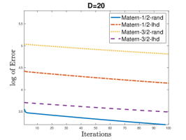
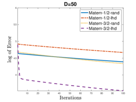
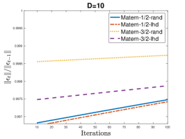

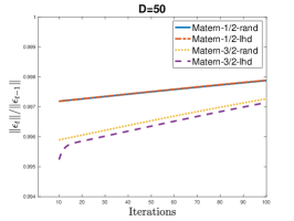
In alignment with Theorem 1, it is established that:
Examination of Figure 3 permits us to ascertain that our empirical findings are in precise agreement with these theoretical lower bounds. In the first row of Figure 3, the slope of the log error curves becomes significantly close to 0 after the initial few iterations. This indicates that once the high-frequency errors are mitigated, the reduction of error attributable to global features becomes remarkably small in each subsequent iteration. In the second row of Figure 3, it is evident that the error ratio starts from a minimum of . Considering our theoretical lower bound for this ratio is and given in our experiments, the observed error ratio of approximately in the experiments aligns closely with our theoretical prediction of .
To summarize, our numerical experiments corroborate the validity of the lower bound established in Theorem 1.
5.2 Comparison on Synthetic Data
In this subsection, we utilize synthetic data to evaluate the performance of our KMG algorithm in comparison to Back-fitting. Following the approach of the previous section, our experiments implement additive Gaussian Processes with both additive-Matérn- and additive-Matérn- kernels, under two distinct scenarios: one involving sampling points distributed randomly within , and another with derived from a Latin Hypercube Design (LHD) within the same domain. Experiments are conducted across dimensions , , and . For each dimension , we let data size . Specifically, data size for dimension , for dimension , and for . Data are generated considering as the effective dimension:
where represents observation noise following a standard normal distribution, effective dimensions set to for , for , and for and each hidden underlying one-dimensional GP employs a kernel function identical to either Mat’ern- or Mat’ern-, which are identical to the kernels utilized by the competing algorithms. Therefore, data are summation of hidden data plus observation noise. The objective for the competing algorithms is to accurately reconstruct the hidden target function from these observations.
The target functions, which serve as the approximation objectives for both KMG and Back-fitting, are defined as
| (29) |
as specified in (21). The competing algorithms are outlined as follows:
-
1.
KMG-rand: Kernel Multigrid with inducing points and sample points distributed uniformly at random within ;
-
2.
KMG-lhd: Kernel Multigrid with inducing points and sample points arranged according to a LHD in ;
-
3.
Backfit-rand: Back-fitting with sample points distributed uniformly at random within ;
-
4.
Backfit-lhd: Back-fitting with sample points on a LHD in .
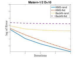
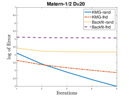


We conduct experiments using the Matérn- kernel and the Matérn- kernel, limiting the number of iterations to before halting all competing algorithms. We evaluate performance by comparing , the vector norm between the outputs of the competing algorithms and the target functions . The results are presented in Figure 4 for the Matérn- kernel and in Figure 5 for the Matérn- kernel, respectively.


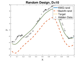


From the upper rows of Figures 4 and 5, it is evident that, even with as few as inducing points, the performance enhancement provided by KMG is significant. Merely 5 iterations suffice for KMG to converge, resulting in an error rate substantially lower than those observed with Back-fitting algorithms.
The middle and lower rows of Figures 4 and 5 underscore the limitations of Back-fitting in converging to the target function. As established in Section 3 and demonstrated through experiments in the preceding subsection, Back-fitting struggles with capturing global features, particularly the true magnitude of the target function. This deficiency is highlighted by the substantial margin of separation between the target function approximations generated by Back-fitting and the actual target function. In contrast, KMG adeptly overcomes this challenge, effectively capturing global features and aligning closely with the true target function, thus demonstrating a superior ability to learn and approximate global characteristics.
To summarize, the experiments presented in this subsection illustrate KMG’s superior efficiency in capturing global features that Back-fitting overlooks. Consequently, KMG significantly enhances the performance of Back-fitting, elevating its efficiency to a new level.
5.3 Real Case Examples
We evaluate the performance of KMG and Back-fitting using the Breast Cancer dataset (Wolberg et al., 1995) and the Wine Quality dataset (Cortez et al., 2009). The Breast Cancer dataset includes 569 samples, each with features, aimed at facilitating breast cancer diagnosis decisions. The Wine Quality dataset comprises 4898 samples, each with features, with the objective of predicting wine quality based on these 11 features.
Our experiments are designed with two primary objectives. The first objective is to assess the accuracy of KMG and Back-fitting in approximating the target function as detailed in (29). This objective is distinct from conventional classification or prediction tasks, as it focuses on reconstructing how each feature contributes to the outcome. The second objective involves comparing the performance of KMG and Back-fitting in practical applications: we evaluate their classification error rate on the Breast Cancer dataset and their mean squared error (MSE) on the Wine Quality dataset. The classification error rate and MSE are defined as follows:
Details of all competing algorithms are outlined as follows:
-
1.
KMG-Mat-1/2: Kernel Multigrid for additive Matén-1/2 kernel with inducing points ;
-
2.
KMG-Mat-3/2: Kernel Multigrid for additive Matén-3/2 kernel with inducing points ;
-
3.
Backfit-Mat-1/2: Back-fitting for additive Matén-1/2 kernel;
-
4.
Backfit-Mat-3/2: Back-fitting for additive Matén-3/2 kernel.
To assess the performance of KMG and Back-fitting in reconstructing the target function outlined in (29), we utilized all 569 samples from the Breast Cancer dataset and 2000 samples from the Wine Quality dataset. Initially, we computed the target function (29) utilizing both the Matérn- and Matérn- kernels. Subsequently, we executed both KMG and Back-fitting algorithms to approximate the components specified in (29). The algorithms were allowed a maximum of 20 iterations. The outcomes of these experiments are shown in Figure 6.


For the Breast Cancer classification, we randomly selected 500 samples for the training set and used the remaining 69 samples for the test set. Similarly, for Wine Quality prediction, we randomly chose 2000 samples as our training set and designated the subsequent 1000 samples for the test set. We then constructed additive predictors by summing the outputs from Back-fitting and KMG after 5, 10, and 20 iterations, respectively. Specifically, the predictors were formulated as
where each represents the estimators of obtained through Back-fitting or KMG. These predictors were then used for classification or prediction on the test sets. Each classification and prediction experiment was conducted 100 times to calculate the average error rate and mean squared error (MSE). The outcomes of experiments for Breast Cancer are shown in Table 1 and those for Wine Quality are shown in Table 2.
Across all real-data experiments, it is evident that KMG significantly outperforms Back-fitting in approximating the target , which denotes the contribution of each dimension to the overall data, across all datasets. These findings are consistent with those from the synthetic data experiments. Nevertheless, when employing the estimators derived from KMG and Back-fitting for classification or prediction tasks, the superiority of KMG over Back-fitting, though present, is not as pronounced as it is in estimating the contributions from each dimension. Estimating the overall model and determining the contributions from each individual dimension are fundamentally different objectives. In estimating the overall model , the precise distribution of global features across various dimensions is less crucial. Even if incorrect allocations occur within the Back-fitting algorithm, as demonstrated in Section 3, the aggregate nature of the summation can neutralize errors from such misallocations. However, accurately identifying the contributions demands exact allocation of global features, where any misallocation can result in significant errors.
| Iteration number | 5 | 10 | 20 |
|---|---|---|---|
| KMG-Mat-1/2 | 0.0922 | 0.0699 | 0.0689 |
| KMG-Mat-3/2 | 0.0837 | 0.0664 | 0.0652 |
| Backfit-Mat-1/2 | 0.1266 | 0.1134 | 0.1004 |
| Backfit-Mat-3/2 | 0.1095 | 0.0932 | 0.0876 |
| Iteration number | 5 | 10 | 20 |
|---|---|---|---|
| KMG-Mat-1/2 | 0.4327 | 0.3521 | 0.3478 |
| KMG-Mat-3/2 | 0.3966 | 0.3472 | 0.3403 |
| Backfit-Mat-1/2 | 0.4815 | 0.4331 | 0.4122 |
| Backfit-Mat-3/2 | 0.4387 | 0.4212 | 0.4313 |
A simple example can demonstrate this phenomenon. Consider a model where , with and , leading to if is orthogonal to . When applying Back-fitting to this model, we have proved that it struggles to accurately discern the global features, which are norms in this case. Essentially, Back-fitting can ascertain that the additive model has an norm of , but it faces challenges in deconstructing this aggregate norm back into the distinct contributions of each . This characteristic of Back-fitting hinders its ability to accurately reconstruct each individual , though it does not significantly impede the reconstruction of the overall model . Conversely, identifying the norm for each dimension can be effectively achieved with a modest number of inducing points, which serve to ”isolate” the data by dimensions, followed by straightforward regression for precise estimations.
To summarize, our real-world experiments demonstrate that KMG notably excels over Back-fitting in reconstructing the individual contributions, , from each dimension. However, when it comes to reconstructing the overall model, the superiority of KMG is less pronounced.
6 Conclusions and Discussion
In this study, we establish a lower bound for the convergence rate of Back-fitting, demonstrating that it struggles to effectively reconstruct global features, necessitating at least iterations to converge. To address this limitation, we propose an enhancement by applying a sparse GPR to the residuals generated by Back-fitting in each iteration. This approach enables the reconstruction of global features and significantly reduces the required number of iterations for convergence to , offering a more efficient solution.
There are several directions that could be pursued in future research. Firstly, the KMG algorithm could be expanded into more advanced Multigrid techniques, such as F-cycles, W-cycles (Saad, 2003), or Multigrid Conjugate Gradients (Tatebe, 1993). For complex real-world challenges, which often involve millions of data points across thousands of dimensions, these potential research directions could yield practical benefits. From a theoretical perspective, the KMG presented in our study, which employs only a small number of inducing points, is sufficient to attain the theoretically fastest exponential convergence rate, while maintaining time and space complexities at minimal order.
Secondly, our focus has been on training additive GPs to reconstruct contributions from each dimension. However, a variety of kernel machines also aim at achieving similar objectives, yet they operate with distinct kernel structure, loss functions, and update mechanisms. Extending our algorithms and analysis to enhance the training efficiency of these diverse models remains an unexplored area.
Thirdly, numerous iterative methods exist for training kernel machines, yet analyses focusing on the requisite number of iterations for these training algorithms are scarce. We posit that there must exist simple modifications to many iterative kernel training methods that could significantly enhance their convergence rates. Similar to our study, it has been rigorously proved that training kernel ridge regression via gradient descent with data augmentation techniques as in Ding et al. (2023), also requires iterations only. Thorough analysis regarding the required iteration number in many other kernel machine training algorithms are needed, presenting an opportunity to broaden our analytical framework and methodology to improve these algorithms.
References
- Ansley and Kohn (1994) C. F. Ansley and R. Kohn. Convergence of the backfitting algorithm for additive models. Journal of the Australian Mathematical Society, 57(3):316–329, 1994.
- Bartels and Hennig (2020) S. Bartels and P. Hennig. Conjugate gradients for kernel machines. Journal of Machine Learning Research, 21(55):1–42, 2020.
- Borzi and Schulz (2009) A. Borzi and V. Schulz. Multigrid methods for pde optimization. SIAM review, 51(2):361–395, 2009.
- Breiman and Friedman (1985) L. Breiman and J. H. Friedman. Estimating optimal transformations for multiple regression and correlation. Journal of the American statistical Association, 80(391):580–598, 1985.
- Brockwell and Davis (1991) P. J. Brockwell and R. A. Davis. Time series: theory and methods. Springer science & business media, 1991.
- Buja et al. (1989) A. Buja, T. Hastie, and R. Tibshirani. Linear smoothers and additive models. The Annals of Statistics, pages 453–510, 1989.
- Burt et al. (2020) D. R. Burt, C. E. Rasmussen, and M. van der Wilk. Variational orthogonal features. arXiv preprint arXiv:2006.13170, 2020.
- Candes and Tao (2007) E. Candes and T. Tao. The dantzig selector: Statistical estimation when p is much larger than n. The Annals of Statistics, 35(6):2313–2351, 2007.
- Chen and Tuo (2022) G. Chen and R. Tuo. Projection pursuit gaussian process regression. IISE Transactions, pages 1–11, 2022.
- Chen et al. (2022) H. Chen, L. Ding, and R. Tuo. Kernel packet: An exact and scalable algorithm for gaussian process regression with matérn correlations. Journal of machine learning research, 23(127):1–32, 2022.
- Chipman et al. (2012) H. A. Chipman, E. I. George, and R. E. McCulloch. Bart: Bayesian additive regression trees. Annals of Applied Statistics, 6(1):266–298, 2012.
- Cockayne et al. (2019) J. Cockayne, C. Oates, I. Ipsen, and M. Girolami. A bayesian conjugate gradient method. Bayesian Analysis, 2019.
- Cortez et al. (2009) P. Cortez, A. Cerdeira, F. Almeida, T. Matos, and J. Reis. Wine Quality. UCI Machine Learning Repository, 2009. DOI: https://doi.org/10.24432/C56S3T.
- Cressie (2015) N. Cressie. Statistics for spatial data. John Wiley & Sons, 2015.
- Cutajar et al. (2016) K. Cutajar, M. Osborne, J. Cunningham, and M. Filippone. Preconditioning kernel matrices. In International conference on machine learning, pages 2529–2538. PMLR, 2016.
- Delbridge et al. (2020) I. Delbridge, D. Bindel, and A. G. Wilson. Randomly projected additive gaussian processes for regression. In International Conference on Machine Learning, pages 2453–2463. PMLR, 2020.
- Ding and Tuo (2024) L. Ding and R. Tuo. A general theory for kernel packets: from state space model to compactly supported basis. arXiv preprint arXiv:2402.04022, 2024.
- Ding and Zhang (2022) L. Ding and X. Zhang. Sample and computationally efficient stochastic kriging in high dimensions. Operations Research, 2022.
- Ding et al. (2023) L. Ding, T. Hu, J. Jiang, D. Li, W. Wang, and Y. Yao. Random smoothing regularization in kernel gradient descent learning, 2023.
- Dutordoir et al. (2020) V. Dutordoir, N. Durrande, and J. Hensman. Sparse gaussian processes with spherical harmonic features. In International Conference on Machine Learning, pages 2793–2802. PMLR, 2020.
- Duvenaud et al. (2011) D. K. Duvenaud, H. Nickisch, and C. Rasmussen. Additive gaussian processes. Advances in neural information processing systems, 24, 2011.
- El-Bachir and Davison (2019) Y. El-Bachir and A. C. Davison. Fast automatic smoothing for generalized additive models. Journal of Machine Learning Research, 20(173):1–27, 2019.
- Eleftheriadis et al. (2023) S. Eleftheriadis, D. Richards, and J. Hensman. Sparse gaussian processes with spherical harmonic features revisited. arXiv preprint arXiv:2303.15948, 2023.
- Fan and Jiang (2005) J. Fan and J. Jiang. Nonparametric inferences for additive models. Journal of the American Statistical Association, 100(471):890–907, 2005.
- Friedman and Stuetzle (1981) J. H. Friedman and W. Stuetzle. Projection pursuit regression. Journal of the American statistical Association, 76(376):817–823, 1981.
- Gardner et al. (2018) J. Gardner, G. Pleiss, K. Q. Weinberger, D. Bindel, and A. G. Wilson. Gpytorch: Blackbox matrix-matrix gaussian process inference with gpu acceleration. Advances in neural information processing systems, 31, 2018.
- Ghandwani et al. (2023) D. Ghandwani, S. Ghosh, T. Hastie, and A. B. Owen. Scalable solution to crossed random effects model with random slopes. arXiv preprint arXiv:2307.12378, 2023.
- Ghosh et al. (2022a) S. Ghosh, T. Hastie, and A. B. Owen. Backfitting for large scale crossed random effects regressions. The Annals of Statistics, 50(1):560–583, 2022a.
- Ghosh et al. (2022b) S. Ghosh, T. Hastie, and A. B. Owen. Scalable logistic regression with crossed random effects. Electronic Journal of Statistics, 16(2):4604–4635, 2022b.
- Gilboa et al. (2013) E. Gilboa, Y. Saatçi, and J. Cunningham. Scaling multidimensional gaussian processes using projected additive approximations. In International Conference on Machine Learning, pages 454–461. PMLR, 2013.
- Hartikainen and Särkkä (2010) J. Hartikainen and S. Särkkä. Kalman filtering and smoothing solutions to temporal gaussian process regression models. In 2010 IEEE international workshop on machine learning for signal processing, pages 379–384. IEEE, 2010.
- Hastie and Tibshirani (2000) T. Hastie and R. Tibshirani. Bayesian backfitting. Statistical Science, 15(3):196–223, 2000.
- Hastie (2017) T. J. Hastie. Generalized additive models. In Statistical models in S, pages 249–307. Routledge, 2017.
- Hensman et al. (2018) J. Hensman, N. Durrande, and A. Solin. Variational fourier features for gaussian processes. Journal of Machine Learning Research, 18(151):1–52, 2018.
- Hestenes et al. (1952) M. R. Hestenes, E. Stiefel, et al. Methods of conjugate gradients for solving linear systems, volume 49. NBS Washington, DC, 1952.
- Kaufman and Sain (2010) C. G. Kaufman and S. R. Sain. Bayesian functional ANOVA modeling using gaussian process prior distributions. Bayesian Analysis, 5(1):123–149, 2010.
- Koltchinskii and Yuan (2010) V. Koltchinskii and M. Yuan. Sparsity in multiple kernel learning. The Annals of Statistics, 38(6):3660 – 3695, 2010.
- Lanczos (1950) C. Lanczos. An iteration method for the solution of the eigenvalue problem of linear differential and integral operators. Journal of Research of the National Bureau of Standards, 45:255–282, 1950.
- Linero (2018) A. R. Linero. Bayesian regression trees for high-dimensional prediction and variable selection. Journal of the American Statistical Association, 113(522):626–636, 2018.
- Loper et al. (2021) J. Loper, D. Blei, J. P. Cunningham, and L. Paninski. A general linear-time inference method for gaussian processes on one dimension. Journal of Machine Learning Research, 22(234):1–36, 2021.
- López-Lopera et al. (2022) A. López-Lopera, F. Bachoc, and O. Roustant. High-dimensional additive gaussian processes under monotonicity constraints. Advances in Neural Information Processing Systems, 35:8041–8053, 2022.
- Lu and McCulloch (2023) X. Lu and R. E. McCulloch. Gaussian processes correlated bayesian additive regression trees. arXiv preprint arXiv:2311.18699, 2023.
- Lu et al. (2022) X. Lu, A. Boukouvalas, and J. Hensman. Additive gaussian processes revisited. In International Conference on Machine Learning, pages 14358–14383. PMLR, 2022.
- Luo et al. (2022) H. Luo, G. Nattino, and M. T. Pratola. Sparse additive gaussian process regression. Journal of Machine Learning Research, 23(61):1–34, 2022.
- Luo (1998) Z. Luo. Backfitting in smoothing spline anova. The Annals of Statistics, 26(5):1733–1759, 1998.
- Maddox et al. (2021) W. J. Maddox, S. Kapoor, and A. G. Wilson. When are iterative gaussian processes reliably accurate? arXiv preprint arXiv:2112.15246, 2021.
- Mammen and Park (2006) E. Mammen and B. U. Park. A simple smooth backfitting method for additive models. The Annals of Statistics, 34(5):2252–2271, 2006.
- Mammen et al. (1999) E. Mammen, O. Linton, and J. Nielsen. The existence and asymptotic properties of a backfitting projection algorithm under weak conditions. The Annals of Statistics, 27(5):1443–1490, 1999.
- McKay et al. (2000) M. D. McKay, R. J. Beckman, and W. J. Conover. A comparison of three methods for selecting values of input variables in the analysis of output from a computer code. Technometrics, 42(1):55–61, 2000.
- Opsomer (2000) J. D. Opsomer. Asymptotic properties of backfitting estimators. Journal of Multivariate Analysis, 73(2):166–179, 2000.
- Paulsen and Raghupathi (2016) V. I. Paulsen and M. Raghupathi. An introduction to the theory of reproducing kernel Hilbert spaces, volume 152. Cambridge university press, 2016.
- Potapczynski et al. (2021) A. Potapczynski, L. Wu, D. Biderman, G. Pleiss, and J. P. Cunningham. Bias-free scalable gaussian processes via randomized truncations. In International Conference on Machine Learning, pages 8609–8619. PMLR, 2021.
- Quinonero-Candela and Rasmussen (2005) J. Quinonero-Candela and C. E. Rasmussen. A unifying view of sparse approximate gaussian process regression. The Journal of Machine Learning Research, 6:1939–1959, 2005.
- Saad (2003) Y. Saad. Iterative methods for sparse linear systems. SIAM, 2003.
- Saatçi (2012) Y. Saatçi. Scalable inference for structured Gaussian process models. PhD thesis, Citeseer, 2012.
- Sadhanala and Tibshirani (2019) V. Sadhanala and R. J. Tibshirani. Additive models with trend filtering. The Annals of Statistics, 47(6):3032–3068, 2019.
- Seeger et al. (2003) M. W. Seeger, C. K. Williams, and N. D. Lawrence. Fast forward selection to speed up sparse gaussian process regression. In International Workshop on Artificial Intelligence and Statistics, pages 254–261. PMLR, 2003.
- Snelson and Ghahramani (2005) E. Snelson and Z. Ghahramani. Sparse gaussian processes using pseudo-inputs. Advances in neural information processing systems, 18, 2005.
- Steinwart and Christmann (2008) I. Steinwart and A. Christmann. Support vector machines. Springer Science & Business Media, 2008.
- Strang (2007) G. Strang. Computational science and engineering. Optimization, 551(563):571–586, 2007.
- Tatebe (1993) O. Tatebe. The multigrid preconditioned conjugate gradient method. In The Sixth Copper Mountain Conference on Multigrid Methods. NASA. Langley Research Center, 1993.
- Titsias (2009) M. Titsias. Variational learning of inducing variables in sparse gaussian processes. In International Conference on Artificial Intelligence and Statistics, pages 567–574. PMLR, 2009.
- Utreras (1988) F. I. Utreras. Convergence rates for multivariate smoothing spline functions. Journal of approximation theory, 52(1):1–27, 1988.
- Wang et al. (2019) K. Wang, G. Pleiss, J. Gardner, S. Tyree, K. Q. Weinberger, and A. G. Wilson. Exact gaussian processes on a million data points. Advances in neural information processing systems, 32, 2019.
- Wendland (2004) H. Wendland. Scattered Data Approximation. Cambridge university press, Cambridge, United Kingdom, 2004.
- Wenger et al. (2021) J. Wenger, G. Pleiss, P. Hennig, J. P. Cunningham, and J. R. Gardner. Reducing the variance of gaussian process hyperparameter optimization with preconditioning. ArXiv, 2107, 2021.
- Wenger et al. (2022a) J. Wenger, G. Pleiss, P. Hennig, J. Cunningham, and J. Gardner. Preconditioning for scalable gaussian process hyperparameter optimization. In International Conference on Machine Learning, pages 23751–23780. PMLR, 2022a.
- Wenger et al. (2022b) J. Wenger, G. Pleiss, M. Pförtner, P. Hennig, and J. P. Cunningham. Posterior and computational uncertainty in gaussian processes. Advances in Neural Information Processing Systems, 35:10876–10890, 2022b.
- Wilson and Nickisch (2015) A. Wilson and H. Nickisch. Kernel interpolation for scalable structured gaussian processes (kiss-gp). In International conference on machine learning, pages 1775–1784. PMLR, 2015.
- Wolberg et al. (1995) W. Wolberg, O. Mangasarian, N. Street, and W. Street. Breast Cancer Wisconsin (Diagnostic). UCI Machine Learning Repository, 1995. DOI: https://doi.org/10.24432/C5DW2B.
- Wu et al. (2023) K. Wu, J. Wenger, H. Jones, G. Pleiss, and J. R. Gardner. Large-scale gaussian processes via alternating projection. arXiv preprint arXiv:2310.17137, 2023.
- Yu et al. (2008) K. Yu, B. U. Park, and E. Mammen. Smooth backfitting in generalized additive models. The Annals of Statistics, 36(1):228–260, 2008.
Appendix A Proof of Lower Bound
In this section, we prove the the propositions and theorems in Section 3. We will first prove Proposition 3 and Proposition 5, then Theorem 6. The final goal is to prove the lower bound in Theorem 1.
Proof [Proposition 3]
Because the Fourier transform of Matérn kernel satisfies
so the Matérn- is proportional to the convolution of the Matérn- and Matérn- kernels:
| (30) |
where is the normalized constant for Fourier transform and, without loss of generality, we can let .
Central KP: From Theorem 3 and Theorem 10 in Chen et al. (2022), the constants for constructing KP are invariant under translation. For example, suppose give the following central KP:
which means that the is non-zero only on .
Recall that Then for any integer , the following central KP
is non-zero only on . Therefore, the central KPs induced by all data points in are translations of each other by multiples of . To prove the proposition for central KPs, we only need to show that it holds for because
for any and half-integer due to the translation invariant property of KPs.
Let , , and . So . If are the coefficients for constructing KP of Matérn- kernel, we can construct KP of Matérn- kernel by solving as follows:
| (31) |
where the third line is from the translation invariance property of KP and the definition of . Because is a KP of Matérn kernel induced by points , it should be non-zero only on according to definition. At any and , we have
| (32) |
| (33) |
We can see that the that satisfy (32) and (33) are
and these are exactly the KP coefficients for Matérn- kernel with three input points . According to the translation invariance property, are also the e KP coefficients for Matérn- kernel with three input points . This finishes the proof for central KPs.
One-sided KP: Let with be the coefficients for constructing left-sided Matérn- KP with input points , i.e.,
is non-zero only on . Let be the coefficients for constructing left-sided Matérn- KP with input points . Here, we only prove the case for constructing left-sided Matérn- KP. The case for right-sided KPs can be proved by following the same reasoning.
Similar to central KP, let and , So and we need to solve for and for left KP as follows:
| (34) |
where now is a left KP for Matérn- kernel, which is supported on . If is a left KP for Matérn- kernel, then for any point , we should have
| (35) |
Similar to central KP, (35) shows that and are the coefficients for Matérn- left KP:
The statement for right KP can be proved in a symmetric way.
Proof [ Proposition 4:] Our strategy is to first construct the following Matérn KP factorization matrix inductively by convolution as Proposition 3:
and
for with the KP factorization matrix for Matérn- kernel as stated in Proposition 1 in Ding and Zhang (2022):
Now we compute the entries on the Matérn KP matrix with . For the central KP of Matérn- kernel, we can have the following KP induced by points through direct calculation:
| (36) |
We now show that central KPs associated to matrix in Proposition 3 is the -time convolution of :
This can be proved by induction. For the base case we already have for Matérn-. Now suppose we have the KP for Matérn-, then for Matérn-, remind that are the coefficients for Matérn- KP, so
Without loss of generality, let be the Matérn- KP induced by points , which is supported on . Using the translation invariant property of KP, we have the following identities for rows of matrix associated to central KPs:
| (37) |
where the last equality is from the fact that is symmetric and is constructed of convolutions of . As a result, is also symmetric.
For the left-sided KP of Matérn- kernel, we can have the following KP induced by points through direct calculation:
Similar to central KPs, suppose we have the left-sided KP for Matérn-, then for Matérn-, remind that are the coefficients for Matérn- KP, so
Without loss of generality, let be the Matérn- left-sided KP induced by points , which is supported on . So using the translation invariant property of KP, we also have
| (38) |
The identity of right-sided KPs can be derived from a similar manner. Now let be the left-sided Matérn- KP induced by points , be the right-sided Matérn- KP induced by points , and be the Matérn- central KP induced by points . By combining (37) and (38), we can have the final result regarding the entries on
Proof [ Proposition 5] We construct the KP matrix that can satisfy the conditions of Proposition 5. We first define the following normalized constants:
where the second equality in each line is because KPs are translation invariant. We can also notice that if we sum over the rows of the KP matrix (over all ) we have the following identity regarding , , and :
| (39) |
Recall that the in Proposition 4 are constructed from the in Proposition 4, i.e. . We now construct the desired from as follows:
| (40) |
Let . Then, it is clear that are also KPs, as each row of consists of coefficients for constructing a KP, and these coefficients, when multiplied by the scalars , , or , remain valid for constructing KPs. Moreover, , , and normalize each summation over rows to :
This finishes the proof for the identity of .
We now estimate the order of each entry of vector . Let as before. From the convolution identities in Proposition 3 and the identities of provided in Proposition 2, it is straightforward to derive that
| (43) |
where the big O for each line is derived directly from Taylor’s expansion.
The last part of the proof is to estimate the order of , , and . For constants and associated to one-sided KPs, because Matérn- one-sided KPs and are supported on and , respectively. Therefore, self-convolutions of and preserve the order of their magnitudes:
| (44) |
For the constant , given that the Matérn- central KP as in (36), and it has support on . So it is straightforward to check by induction that the -time self-convolution of , which is a KP for the Matérn- kernel, has magnitude as follows:
| (45) |
for some universal constant .
Proof [ Theorem 6] We first prove the theorem when kernel is Matérn- kernel. From Proposition 4, we have
| (46) |
For notation simplicity, let . From Woodbury Matrix identity, we have
where the second line is because is positive definite, the third line is from (46), and the last line is from the estimation in Proposition 5 for the entries of . This finishes the prove for Matérn kernel.
For other kernel satisfying Assumption 2.1, i.e., where , we can show that the spectrum of are lower bounded by those of the Matérn- kernel matrix :
for any where and are some universal constant independent of kernel and . So .
Proof [Theorem 1:] We only need to show that after iterations, error reduced by the error form is lower bounded as follows:
We first define the following unit vector in :
Recall that the Back-fit operator . Let be any -dimensional vector for such that
Then, we can notice that the block Gauss-Seidel iteration gives
Substitute , we can immediately get
where
On the other hand . So we have
where the last line is from the fact that the third line is exactly the error for the two-dimensional counterexample in Section 3.4.
Because is a normalized vector, we can conclude that the largest eigenvalue of the Back-fit operator is greater than :
Let be the eigenvector associated to the largest eigenvalue . Then the projection of initial error onto can be lower bounded simply as follows:
It can be directly deduced that in each iteration, at most a fraction of the error projected onto is eliminated. By induction, the fraction of error eliminated after iterations is at most :
Appendix B Approximation Property of Sparse Additive GPR
We first introduce lemmas that will be used in our later proof.
B.1 Useful Lemmas
Lemma 15 (Corollary 10.13 in Wendland (2004))
Let be RKHS induced by one-dimensional kernel satisfying Assumption (2.1). Then is equivalent to the -th order Sobolev space:
Lemma 16 (Theorem 3.3 & 3.4 in Utreras (1988))
Let be the -th order Sobolev space. Let be any point set satisfying the following fill distance condition:
| (47) |
for some value . Then for any function , we have
where denote the Sobolev norm associated to , and are some constants independent of and .
From Lemma 16, we can derive the following error estimate for one-dimensional interpolation.
Lemma 17
Proof Let denote the interpolator . From the representation theorem, we have
Obviously, . From Lemma 15, we know that is equivalent to the -th order Sobolev space . We the can directly have the result from Lemma 16.
The following Lemma highlights key geometric characteristics commonly employed in the theory of sparse recovery, notably the concept of ”restricted isometry constants” as introduced in Candes and Tao (2007). We adopt its kernel version as proposed by Koltchinskii and Yuan (2010).
Lemma 18 (Proposition 1 in Koltchinskii and Yuan (2010))
Let be any distribution on . Let be one-dimensional kernel satisfying Assumption 2.1. For any linear independent functions , let be the gram matrix induced by . Let be the minimum eigenvalue of . Define
| (48) |
Then for any , we have
From Lemma 18, we can derive the following sampling inequality for function of additive form .
Lemma 19
Proof For any , it must be in the form
Then, the sup norm of can be bounded as follows:
where the third line is from Lemma 15 and Gagliardo–Nirenberg interpolation inequality, the fourth line is from Lemma 16, the fifth line is from Höler inequality, and the last line is from Lemma 18.
B.2 Main Proof of Theorem 7
Equipped with Lemmas introduced in the previous subsection, we now can start our proof for Theorem 7.
Proof [ Theorem 7] For any function , we define the following vector as the values of on the data points :
So the RKHS norm of is
and we can also define the following vector as the values of on the inducing points :
The equation can be written as
| (49) |
We define , and substitute into (49):
| (50) | |||
| (51) |
For and , we can use Lemma 16 and Lemma 17 to show that
| (52) |
We now estimate the in (51). Multiply it by :
| (53) |
where and are low-rank kernel matrices:
Let and
We can notice that the matrix in (53) has the following identities for all its entries
and for any , we have
so we can bound the empirical norm of each as follows:
| (54) |
For any function , we define the following linear operator for notation convenient:
Obviously, is also in and
Then using Lemma 19, we have for any :
| (55) |
where the last line is from (54) and direct calculations.
It is straightforward to check that is positive definite. So for any , we have
Also, because, obviously, spectrum of is less than 1. So
From previous calculations, we have already known . So
| (56) |
Substitute (56) into (55), and remind that , we can have
It is straightforward to check that for any , is a positive definite kernel. As a result, for any , we can derive the following upper bound:
| (57) |
Substitute(57) into (53), we can have
| (58) |
where the last line is from (52). Then we can apply Lemma 18 on (58) to have the following upper bound for (51):
| (59) |
The final part of our proof is to estimate in (51). Let
So . From Theorem 16, it is straightforward to derive the following sampling inequality
| (60) |
Obviously, so we only need to estimate the RKHS norm of . From long but straightforward calculations, we can have
| (61) |
where and the fourth line is from the Neumann series expansion for .
Appendix C Convergence Rate of Kernel Multigird
C.1 Smoothing Property of
Proof [Lemma 10] We first write the Back-fit operator in error form . Denote the error in the -th iteration as where corresponds to the error of dimension . Then each Back-fitting iteration can be written a
| (64) |
From (64), we can notice that can be viewed as the values of a kernel ridge regression on : such that
| (65) |
Moreover, from the representation theorem, we must have the following equality regarding the RKHS norm of :
Obviously is a feasible solution of (65). Because is the minimum of (65), we must have
| (66) |
where the second line is from Jensen’s inequality and the convexity of norm and the last line is because Back-fitting converges so we must have for any and . As a result, the RKHS norm for the error of the -th iteration is
where the last line is from (66).
According to definition, , we can finish the proof.