AFLoRA: Adaptive Freezing of Low Rank Adaptation in Parameter Efficient Fine-Tuning of Large Models

Abstract

We present a novel Parameter-Efficient Fine-Tuning (PEFT) method, dubbed as Adaptive Freezing of Low Rank Adaptation (AFLoRA). Specifically, for each pre-trained frozen weight tensor, we add a parallel path of trainable low-rank matrices, namely a down-projection and an up-projection matrix, each of which is followed by a feature transformation vector. Based on a novel freezing score, we the incrementally freeze these projection matrices during fine-tuning to reduce the computation and alleviate over-fitting. Our experimental results demonstrate that we can achieve state-of-the-art performance with an average improvement of up to $0.85\%$ as evaluated on GLUE benchmark while yeilding up to $9.5\times$ fewer average trainable parameters. While compared in terms of runtime, AFLoRA can yield up to $1.86\times$ improvement as opposed to similar PEFT alternatives. Besides the practical utility of our approach, we provide insights on the trainability requirements of LoRA paths at different modules and the freezing schedule for the different projection matrices. Code will be released.

1 Introduction

Pre-trained language models such as BERT (Devlin et al., 2018), GPT-3 (Brown et al., 2020), and LLaMA2 (Touvron et al., 2023) have demonstrated commendable performance on various natural language processing (NLP) tasks. However, their zero-shot performance on many downstream tasks often falls short of expectations. One possible solution is full fine-tuning (FFT) of the model on the downstream dataset. However, the large model parameter size makes this process prohibitively costly.

To address this challenge, various parameter-efficient fine-tuning (PEFT) methods including low rank adaptation (LoRA) (Hu et al., 2021), adapter tuning (He et al., 2021), and prompt tuning (Lester et al., 2021) are proposed. These methods add parameters to the trained model for fine-tuning, bypassing the need to adjust the weights of the pre-trained model. In particular, LoRA (Hu et al., 2021) and its variants (Zhang et al., 2023) add a trainable low-rank path consisting of down-projection and up-projection matrices to the model, inspired by Aghajanyan et al. (2020) which showed that such low-rank paths can effectively approximate the trained weight tensors. ELoRA Kopiczko et al. (2024) extends LoRA by adding trainable feature transformation vectors to the output of each project matrix. They showed that SoTA accuracy can be achieved with the projection matrices frozen after random initialization while keeping the two feature transformation vectors trainable. This approach significantly reduces the number of trainable parameters. However, compared to LoRA, ELoRA incurs higher computation costs due to higher rank needed for the frozen projection matrices. Fig. 1 illustrates LoRA and ELoRA, contrasting them to our proposed method AFLoRA.

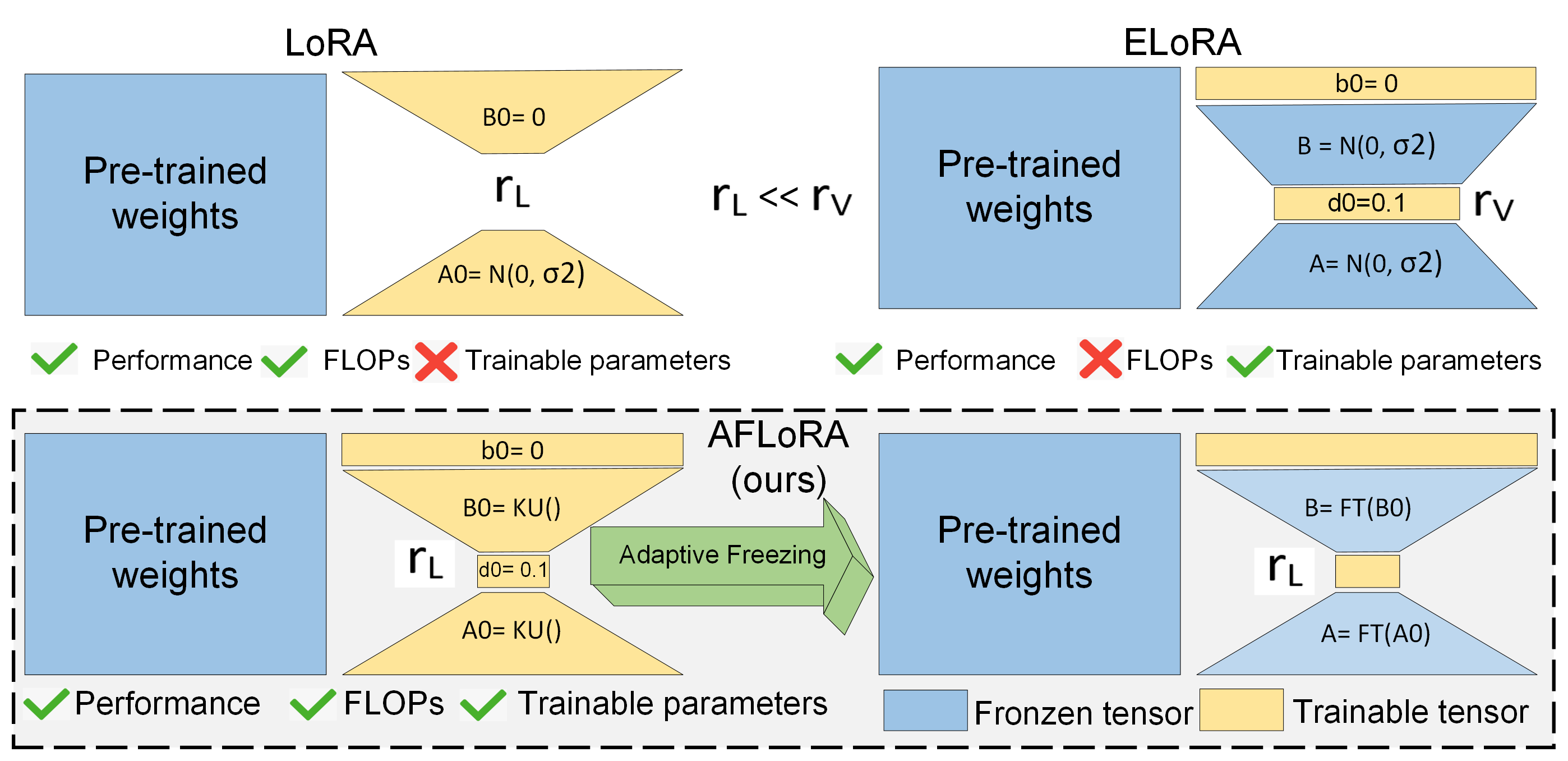
Figure 1: Schematic comparison of LoRA (Hu et al., 2021), ELoRA (Kopiczko et al., 2024), and AFLoRA and their associated advantages and disadvantages in terms of various metrics. $r_{L}$ and $r_{V}$, represent rank of the low rank path used in LoRA and ELoRA methods, respectively. FT and KU refers to fine-tuned weights and Kaiming uniform initialization function, respectively.

Our contributions. To reduce the trainable parameter count and computation costs of fine-tuning, we present Adaptive Freezing of Low Rank Adaptation (AFLoRA). More specifically, we first investigate the rank needed for the frozen LoRA path in ELoRA and observe that reducing the rank of the frozen projection matrices (PM) causes a drop in fine-tuning performance.

Based on this insight, we present AFLoRA, that starts with a low-rank trainable path that includes projection matrices and feature transformation vectors and train the path for some epochs. We then gradually freeze the projection matrices based on a novel freezing score that acts as a proxy for the trainability requirement of a LoRA tensor. In this way, we not only help alleviate the over-fitting issue but also, improve the computation efficiency. To evaluate the benefit of AFLoRA, we perform extensive evaluations on multiple NLP benchmark datasets and compare accuracy, FLOPs, and training time with several existing alternatives. In specific, compared to ELoRA we yield $1.86\times$ and $2.96\times$ improvement in runtime and FLOPs, respectively, while remain comparable as LoRA on these two metrics. Compared to LoRA we require $9.5\times$ fewer average trainable parameters to yield similar or improved performance.

2 Related Works

PEFT (Hu et al., 2021; Kundu et al., 2024) refers to a collection of methodologies that focus on allowing a small number of parameters to fine-tune to yield good performance on a downstream task. For example, prefix-tuning (Li and Liang, 2021) adds trainable prefix tokens to a model’s input or hidden layers while adapter-tuning (Houlsby et al., 2019) inserts small neural network layers, known as adapters, within each layer of a pre-trained model. LoRA (Hu et al., 2021), on the other hand, adds low-rank tensors in parallel to the frozen pre-trained weights. AdaLoRA (Zhang et al., 2023) allows the rank of the LoRA path to be chosen in an adaptive way. Other variants like SoRA Ding et al. (2023) and LoSparse Li et al. (2023) have investigated the impact of sparsity in and alongside the low-rank path, respectively. Recently, efficient low-rank adaptation (ELoRA) (Kopiczko et al., 2024) has proposed to keep the LoRA path frozen, while introducing two trainable feature transformation vectors. Thus, this work only studies an extreme scenario of keeping the LoRA path frozen, and, to the best of our knowledge, no work has investigated the trainability requirement of the projection matrices.

3 Motivational Case Study

To understand the high rank requirement for the frozen projection metrices in ELoRA, we conduct two sets of fine-tuning on SST-2 and MRPC, with ELoRA having rank ($r$) of 1024 and 4, respectively. As we can see in Fig. 2, the model with $r=4$, yields poorer performance, highlighting the need for high rank for the frozen tensors. This high rank causes ELoRA to potentially be FLOPs inefficient.

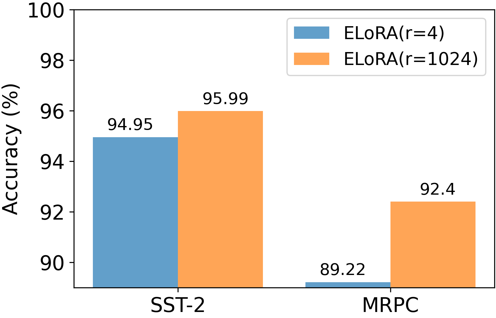
Figure 2: Performance of ELoRA with two different ranks of the frozen projection matrices.

4 AFLoRA: Methodology

Table 1: Comparison of different LoRA variants with DeBERTaV3 on the GLUE benchmark.

Method	#Params. $\downarrow$	CoLA $\uparrow$	SST-2 $\uparrow$	MRPC $\uparrow$	QNLI $\uparrow$	STS-B $\uparrow$	RTE $\uparrow$	MNLI $\uparrow$	QQP $\uparrow$	Avg. $\uparrow$
FFT	184M	69.21	95.64	89.22	93.78	91.59	82.49	89.98/89.95	92.05/89.31	87.82
LoRA (r = 8)	1.33M	69.73	95.57	89.71	93.76	91.86	85.32	90.47/90.46	91.95/89.26	88.38
AdaLoRA	1.27M	70.86	95.95	90.22	94.28	91.39	87.36	90.27/90.30	92.13/88.41	88.83
SoRA (r = 4)	0.47M	71.05	95.57	90.20	93.92	91.76	86.04	90.38/90.43	92.06/89.44	88.71
ELoRA*	0.16M	70.74	95.18	90.93	93.58	91.08	87.36	90.11/90.22	90.69/87.63	88.53
AFLoRA (r = 4)	0.14M**	72.01	96.22	91.91	94.42	91.84	88.09	89.88/90.17	90.81/87.77	89.23

• * The original paper has results with the RoBERTa, we generated the results with our implementation on DeBERTaV3 with rank of 1024.

• ** As the number of trainable parameters is changed during training, we computed this by averaging over the whole training epochs over all datasets.

Module Structure. Inspired by the framework proposed by Kopiczko et al. (2024), we design the LoRA module to encompass four components, namely, the down-projection linear layer ($lora_{A}$), the up-projection linear layer ($lora_{B}$), and two feature transform vectors ($s_{d}$, and $s_{b}$) placed before and after $lora_{B}$. However, unlike Kopiczko et al. (2024), we keep both the projection matrices ($lora_{A}$ and $lora_{B}$) and vectors trainable at the beginning and keep the rank very low. The module processes a given input $X$ through these components to produce an output $Y$. The complete operation for a layer $l$ can be described as follows:

$${Y}={W^{l}_{0}}{X}+\Lambda^{l}_{b}B^{l}\Lambda^{l}_{d}A^{l}{X}$$ (1)

Here, $A^{l}$ and $B^{l}$ are the trainable LoRA tensors of $lora^{l}_{A}$ and $lora^{l}_{B}$, respectively. $\Lambda_{d}$ and $\Lambda_{b}$ are the vectors of $s_{d}$, and $s_{b}$, respectively. $W^{l}_{0}$ represents the frozen pre-trained weights. We use Kaiming Uniform initialization for $A^{l}$ and $B^{l}$, and follow Kopiczko et al. (2024) to initialize the vectors.

Adaptive Freezing. In pruning literature (Han et al., 2015; Molchanov et al., 2019; Zhang et al., 2022), sensitivity is gauged to reflect weight variability, necessitating consideration of both the weights’ magnitudes and their gradients. Small weight values suggest minimal impact, while minor gradient values indicate stability. Taking inspiration from this idea, here we introduce the concept of a "freezing score". However, unlike pruning where both magnitude and gradient play a critical role to identify insignificant weight, we leverage only gradient as a proxy to compute the freezing score. This is because, we assume large magnitude weights with negligible change has same priority to be frozen as that for small magnitude weights. This score quantifies the degree to which weights vary throughout the training process. Consequently, when the expected changes to the weights become negligible, we may consider them to be frozen, thereby saving computational resources and energy.

Following equation describes the freezing score evaluation steps for a low-rank tensor $A^{l}$.

$$I_{A^{l}}=\left|\nabla\mathcal{L}(\boldsymbol{\theta)}\right|,\overline{I}_{A^{l}}^{(t)}=\beta_{1}\overline{I}_{A^{l}}^{(t-1)}+(1-\beta_{1})I_{A^{l}}^{(t)}$$ (2)

$$U_{A^{l}}^{(t)}=\left|I_{A^{l}}^{(t)}-\overline{I}_{A^{l}}^{(t)}\right|,\overline{U}_{A^{l}}^{(t)}=\beta_{2}\overline{U}_{A^{l}}^{(t-1)}+(1-\beta_{2})U_{A^{l}}^{(t)}$$ (3)

$$s_{A^{l}}^{(t)}=mean(\overline{I}_{A^{l}}^{(t)}\circ\overline{U}_{A^{l}}^{(t)})$$ (4)

Here, for each projection tensor at iteration $t$, we compute a smoothed gradient ($\overline{I}_{A^{l}}^{(t)}$) and uncertainly tensor ($\overline{U}_{A^{l}}^{(t)}$), as shown in Eq. 2 and 3, respectively. We then evaluate the freezing score $s_{A^{l}}^{(t)}$, as the mean of the tensor generated via Hadamard product ($\circ$) between $\overline{I}_{A^{l}}^{(t)}$ and $\overline{U}_{A^{l}}^{(t)}$.

To apply thresholding on the LoRA freezing scores, we use the cubic schedule as (Zhang et al., 2022). In specific, we keep the projection matrices trainable for the initial $t_{i}$ training steps, and then progessively freeze them by calculating the freezing fraction $r(t)$ as shown in the Eq. 5. Finally all the projection matrices freeze beyond $T-t_{f}$ steps. Note, at a step $t$, for a computed freezing fraction $k$, we freeze the lowest $k\%$ projection matrices.

$$r(t)=\left\{\begin{array}[]{ll}0&\quad 0\leq t<t_{i}\\ 1-\left(1-\frac{t-t_{i}}{T-t_{i}-t_{f}}\right)^{3}&\quad t_{i}\leq t<T-t_{f}\\ 1&\quad\text{otherwise}\end{array}\right.$$ (5)

where $t$ refers to current #step, $T$ is the total number of fine-tuning steps. We set $t_{i}$ to the steps corresponding to one epoch and set $t_{f}$ to 70% of the total training steps.

5 Experiments

Models & Datasets. We use the PEFT framework of Mangrulkar et al. (2022) and evaluate the fine-tuning performance of DeBERTaV3-base (He et al., 2020) to fine-tune on our framework on the General Language Understanding Evaluation (GLUE) benchmark (Wang et al., 2018). The details of the hyperparameter settings for each dataset are listed in Appendix A.2.

Performance Comparison. We benchmark the performance with AFLoRA and present comparison with LoRA and its variants. For ELoRA, we reproduce the results at our end while the results for other methods are sourced from Ding et al. (2023). As shown in Table 1, AFLoRA can achieve SoTA performance on majority of datasets and on average while requiring similar and $9.5\times$ fewer average trainable parameters as compared to ELoRA and LoRA, respectively.

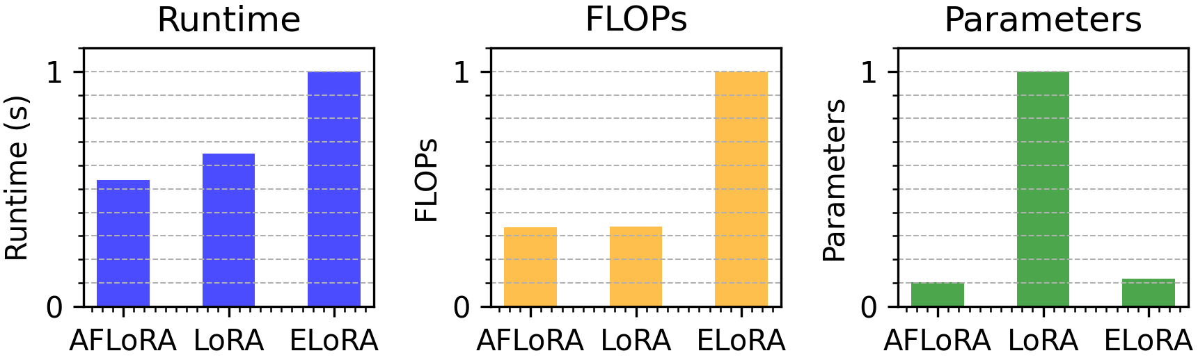
Figure 3: A comparison of various system performance between LoRA, ELoRA, and AFLoRA.

Runtime & FLOPs Comparison. Fig. 3 shows the comparison of the normalized average training runtime, normalized FLOPs, and normalized trainable parameters. For AFLoRA, we average the training time, FLOPs, and trainable parameters over six GLUE datasets (except the MNLI and QQP datasets). Note, for LoRA and ELoRA, the trainable parameters and FLOPs remain fixed for all the dataset. We compute their average runtime same way as ours. Compared to ELoRA we can yield up to $1.86\times$ and $2.96\times$ runtime and FLOPs improvement while remain comparable with LoRA in these two metrices. Compared to LoRA we yield $9.5\times$ parameter reduction, while remain comparable with ELoRA. These results clearly demonstrate AFLoRA as PEFT method that can yield similar parameter efficiency as ELoRA while costing no training overhead in terms of FLOPs or time.

6 Ablations and Discussions

We conducted our ablation studies on six GLUE benchmark datasets, omitting QQP and MNLI, the two most computationally demanding datasets.

Do we really need adaptive freezing? We conducted experiments with all the LoRA PMs frozen (same as ELoRA), all the LoRA PMs trainable, and with our adaptive training of LoRA PMs. We use, $r=4$ for the LoRA path, for all. As we can see in Table 2, keeping the projection matrices trainable yield better average performance compared to keeping them frozen throughout. However, AFLoRA with adaptive freezing yields even better performance than keeping them trainable throughout, potentially highlighting its ability to regularize the fine-tuning against overfitting.

Table 2: Ablation study on the trainability impact of the projection matrices (PM) of the AFLoRA module. We keep the vectors trainable throughout for all.

PM	#Params.	CoLA	SST-2	MRPC	QNLI	STS-B	RTE	Avg.
Trainable	0.45M	70.15	95.99	92.4	94.16	89.90	88.45	88.51
Frozen	0.08M	70.36	94.95	89.22	93.61	91.17	85.92	87.54
AFLoRA (Ours)	0.14M	72.01	96.22	91.91	94.42	91.84	88.09	89.23

Do we need to keep the PMs trainable for all layer types? There are two major layer types, FFN and the attention layers. We place the PMs in both along with the feature transformation vectors. We then study the necessity of keeping the PMs trainable in these two layer types. Note, here, we keep the vectors trainable for all throughout. As shown in Table 3, keeping the PMs trainable (and then adaptive freezing) in the FFN yields better performance compared to the alternatives. Note we keep the PMs in the attention layers frozen to random values. Interestingly, allowing all PMs to initially train and then adaptively freeze yields poorer performance than allowing them only in MLP. This may hint at the FFN weights to play more important role in fine-tune performance.

Table 3: Ablation study on making the PMs for different layer-types trainable.

FFN	Attn	CoLA	SST-2	MRPC	QNLI	STS-B	RTE	Avg.
✓	✓	70.33	95.76	90.93	94.36	91.44	87.37	88.48
		0.15M	0.19M	0.18M	0.19M	0.16M	0.17M	0.17M
✗	✓	71.118	95.986	89.951	94.12	91.39	86.28	88.14
		0.11M	0.13M	0.12M	0.13M	0.12M	0.12M	0.12M
✓	✗	72.01	96.22	91.91	94.42	91.84	88.09	89.02
		0.13M	0.18M	0.13M	0.13M	0.13M	0.13M	0.14M

Ablation with sensitivity choices. Fig. 4 presents ablation with three sensitivity scores based on three different sensitivity choices, namely, $|grad(p)|$ (adopted in AFLoRA), $|p*grad(p)|$, and $|grad(p)/p|$. On average, the freezing score adopted in AFLoRA, consistently yield better accuracy over the other two.

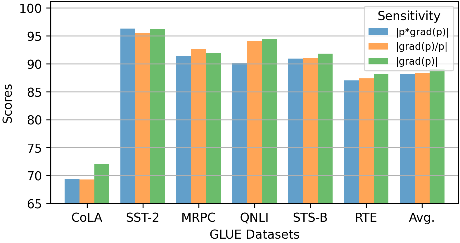
Figure 4: A comparison of performance outcomes utilizing three distinct freezing score methodologies.

Discussion on Freezing Trend. We use the RTE dataset as a case study, to understand the freezing trend of the PMs across different layers. In specific, we illustrate the specific number of iterations required before freezing each component in Fig.5. Interestingly, as can be seen from the figure, analysis reveals that the down-projection matrix parallel the intermediate linear layer require longer training duration prior to being frozen, as compared to the other PMs. This may potentially hint at the low approximation ability of the intermediate layer as compared to the second MLP in the FFN.

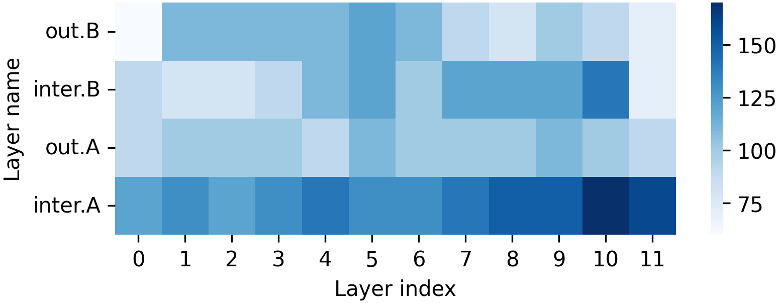
Figure 5: Visualization of freezing iterations for each layer. ‘out’ and ‘inter’ refer to the second and the first MLP layer of the FFN, respectively. ‘A’ and ‘B’ represent the down-projection and up-projection matrix, respectively. The darker the color, the more iterations the matrix has to go through before freezing.

7 Conclusions

In this paper we presented AFLoRA, an adaptive freezing of LoRA adapters that allow near optimal trainability of the LoRA projection matrices and freezes them driven by a "freezing score" after certain fine-tuning steps. Compared to LoRA, AFLoRA can reduce the trainable parameters by up to $9.5\times$ while yielding $0.85\%$ average imporved performance as evaluated on GLUE benchmark.

8 Limitation

In the ablation study with various freezing score metrics, we discovered that alternative scoring methods outperform ours on certain datasets, suggesting possible room for research in refining the freezing scores. This can further improve performance with AFLoRA. Additionally, integration of AFLoRA in the adaptive rank evaluation framework can potentially open a new direction of PEFT that we consider as a future research.

Appendix A Appendix

A.1 Dataset

The details of train/test/dev splits and the evaluation metric of the GLUE (Wang et al., 2018) dataset are reported in Table 4. We use the Huggingface Transformers library Wolf et al. (2020) to source all the datasets.

Table 4: Statistics of the GLUE benchmark datasets."Mcc", "Acc", "F1" and "Pear" represent Matthews correlation coefficient, accuracy, the F1 score and the Pearson correlation coefficient respectively. And "Acc" for MNLI dataset contains the accuracy for the matched and mismatched subset of the datasets.

Dataset	#Train	#Valid	#Test	Metric
CoLA	8.5k	1,043	1,063	Mcc
SST-2	67k	872	1.8k	Acc
MRPC	3.7k	408	1.7k	Acc
QQP	364k	40.4k	391k	Acc/F1
STS-B	5.7k	1.5k	1.4k	Pear
MNLI	393k	9.8k/9.8k	9.8k/9.8k	Acc
QNLI	105k	5.5k	5.5k	Acc
RTE	2.5k	277	3k	Acc

A.2 Hyperparameter configuration

Table 5 shows the main hyper-parameter setup in this paper. Besides them, we use the same optimizer, warmup Ratio, and LR schedule as Hu et al. (2021). We use NVIDIA RTX A6000 (maximum GPU memory=49140MB) to measure the training runtime. For all experiments, we run 5 times using different random seeds and report the average results.

Table 5: Hyperparameter setup for all eight datasets in GLUE benchmark

Hyperparameter	CoLA	SST-2	MRPC	QNLI	STS-B	RTE	MNLI	QQP
# epochs	20	10	20	10	20	20	10	10
Batch size	64
Max Seq. Len.	256
Clf. Lr.*	4E-2	4E-3	8E-2	4E-3	2E-2	4E-2	4E-3	4E-3
Learning rate	1E-2	4E-3	1E-2	1E-3	2E-3	1E-3	1E-3	4E-3
$t_{i}(epoch)$	1
$t_{f}(epoch)$	14	7	14	7	14	14	7	7
$\beta_{1}$	0.85
$\beta_{2}$	0.95

• * "Clf. Lr.*" means the learning rate for the classification head.

A.3 Ablation study on if freezing the two projection matrices in the same layer simultaneously

We study the value of freezing both projection matrices in the same layer simultaneously. The results, depicted in Table 6, demonstrate that freezing the projection matrices separately yields consistently superior performance compared to freezing them simultaneously.

Table 6: Ablation study on whether freezing the two projection matrices in the same layer simultaneously or independently.

	Simultaneously	Independently
CoLA	67.90	72.01
SST-2	95.87	96.22
MRPC	91.67	91.91
STS-B	91.64	91.84
QNLI	94.20	94.42
RTE	87.00	88.09
Avg.	88.05	89.02
#Params	0.146M	0.138M

References

- Aghajanyan et al. (2020) Armen Aghajanyan, Luke Zettlemoyer, and Sonal Gupta. 2020. Intrinsic dimensionality explains the effectiveness of language model fine-tuning. arXiv preprint arXiv:2012.13255.
- Brown et al. (2020) Tom Brown, Benjamin Mann, Nick Ryder, Melanie Subbiah, Jared D Kaplan, Prafulla Dhariwal, Arvind Neelakantan, Pranav Shyam, Girish Sastry, Amanda Askell, et al. 2020. Language models are few-shot learners. Advances in neural information processing systems, 33:1877–1901.
- Devlin et al. (2018) Jacob Devlin, Ming-Wei Chang, Kenton Lee, and Kristina Toutanova. 2018. Bert: Pre-training of deep bidirectional transformers for language understanding. arXiv preprint arXiv:1810.04805.
- Ding et al. (2023) Ning Ding, Xingtai Lv, Qiaosen Wang, Yulin Chen, Bowen Zhou, Zhiyuan Liu, and Maosong Sun. 2023. Sparse low-rank adaptation of pre-trained language models. arXiv preprint arXiv:2311.11696.
- Han et al. (2015) Song Han, Jeff Pool, John Tran, and William Dally. 2015. Learning both weights and connections for efficient neural network. Advances in neural information processing systems, 28.
- He et al. (2020) Pengcheng He, Xiaodong Liu, Jianfeng Gao, and Weizhu Chen. 2020. Deberta: Decoding-enhanced bert with disentangled attention. arXiv preprint arXiv:2006.03654.
- He et al. (2021) Ruidan He, Linlin Liu, Hai Ye, Qingyu Tan, Bosheng Ding, Liying Cheng, Jia-Wei Low, Lidong Bing, and Luo Si. 2021. On the effectiveness of adapter-based tuning for pretrained language model adaptation. arXiv preprint arXiv:2106.03164.
- Houlsby et al. (2019) Neil Houlsby, Andrei Giurgiu, Stanislaw Jastrzebski, Bruna Morrone, Quentin De Laroussilhe, Andrea Gesmundo, Mona Attariyan, and Sylvain Gelly. 2019. Parameter-efficient transfer learning for nlp. In International Conference on Machine Learning, pages 2790–2799. PMLR.
- Hu et al. (2021) Edward J Hu, Yelong Shen, Phillip Wallis, Zeyuan Allen-Zhu, Yuanzhi Li, Shean Wang, Lu Wang, and Weizhu Chen. 2021. Lora: Low-rank adaptation of large language models. arXiv preprint arXiv:2106.09685.
- Kopiczko et al. (2024) Dawid Jan Kopiczko, Tijmen Blankevoort, and Yuki M Asano. 2024. ELoRA: Efficient low-rank adaptation with random matrices. In The Twelfth International Conference on Learning Representations.
- Kundu et al. (2024) Souvik Kundu, Sharath Sridhar Nittur, Maciej Szankin, and Sairam Sundaresan. 2024. Sensi-bert: Towards sensitivity driven fine-tuning for parameter-efficient bert. ICASSP.
- Lester et al. (2021) Brian Lester, Rami Al-Rfou, and Noah Constant. 2021. The power of scale for parameter-efficient prompt tuning. arXiv preprint arXiv:2104.08691.
- Li and Liang (2021) Xiang Lisa Li and Percy Liang. 2021. Prefix-tuning: Optimizing continuous prompts for generation. arXiv preprint arXiv:2101.00190.
- Li et al. (2023) Yixiao Li, Yifan Yu, Qingru Zhang, Chen Liang, Pengcheng He, Weizhu Chen, and Tuo Zhao. 2023. Losparse: Structured compression of large language models based on low-rank and sparse approximation. arXiv preprint arXiv:2306.11222.
- Mangrulkar et al. (2022) Sourab Mangrulkar, Sylvain Gugger, Lysandre Debut, Younes Belkada, Sayak Paul, and Benjamin Bossan. 2022. Peft: State-of-the-art parameter-efficient fine-tuning methods. https://github.com/huggingface/peft.
- Molchanov et al. (2019) Pavlo Molchanov, Arun Mallya, Stephen Tyree, Iuri Frosio, and Jan Kautz. 2019. Importance estimation for neural network pruning. In Proceedings of the IEEE/CVF conference on computer vision and pattern recognition, pages 11264–11272.
- Touvron et al. (2023) Hugo Touvron, Louis Martin, Kevin Stone, Peter Albert, Amjad Almahairi, Yasmine Babaei, Nikolay Bashlykov, Soumya Batra, Prajjwal Bhargava, Shruti Bhosale, Dan Bikel, Lukas Blecher, Cristian Canton Ferrer, Moya Chen, Guillem Cucurull, David Esiobu, Jude Fernandes, Jeremy Fu, Wenyin Fu, Brian Fuller, Cynthia Gao, Vedanuj Goswami, Naman Goyal, Anthony Hartshorn, Saghar Hosseini, Rui Hou, Hakan Inan, Marcin Kardas, Viktor Kerkez, Madian Khabsa, Isabel Kloumann, Artem Korenev, Punit Singh Koura, Marie-Anne Lachaux, Thibaut Lavril, Jenya Lee, Diana Liskovich, Yinghai Lu, Yuning Mao, Xavier Martinet, Todor Mihaylov, Pushkar Mishra, Igor Molybog, Yixin Nie, Andrew Poulton, Jeremy Reizenstein, Rashi Rungta, Kalyan Saladi, Alan Schelten, Ruan Silva, Eric Michael Smith, Ranjan Subramanian, Xiaoqing Ellen Tan, Binh Tang, Ross Taylor, Adina Williams, Jian Xiang Kuan, Puxin Xu, Zheng Yan, Iliyan Zarov, Yuchen Zhang, Angela Fan, Melanie Kambadur, Sharan Narang, Aurelien Rodriguez, Robert Stojnic, Sergey Edunov, and Thomas Scialom. 2023. Llama 2: Open foundation and fine-tuned chat models.
- Wang et al. (2018) Alex Wang, Amanpreet Singh, Julian Michael, Felix Hill, Omer Levy, and Samuel R Bowman. 2018. Glue: A multi-task benchmark and analysis platform for natural language understanding. arXiv preprint arXiv:1804.07461.
- Wolf et al. (2020) Thomas Wolf, Lysandre Debut, Victor Sanh, Julien Chaumond, Clement Delangue, Anthony Moi, Pierric Cistac, Tim Rault, Remi Louf, Morgan Funtowicz, Joe Davison, Sam Shleifer, Patrick von Platen, Clara Ma, Yacine Jernite, Julien Plu, Canwen Xu, Teven Le Scao, Sylvain Gugger, Mariama Drame, Quentin Lhoest, and Alexander Rush. 2020. Transformers: State-of-the-art natural language processing. In Proceedings of the 2020 Conference on Empirical Methods in Natural Language Processing: System Demonstrations, pages 38–45, Online. Association for Computational Linguistics.
- Zhang et al. (2023) Qingru Zhang, Minshuo Chen, Alexander Bukharin, Pengcheng He, Yu Cheng, Weizhu Chen, and Tuo Zhao. 2023. Adaptive budget allocation for parameter-efficient fine-tuning. In The Eleventh International Conference on Learning Representations.
- Zhang et al. (2022) Qingru Zhang, Simiao Zuo, Chen Liang, Alexander Bukharin, Pengcheng He, Weizhu Chen, and Tuo Zhao. 2022. Platon: Pruning large transformer models with upper confidence bound of weight importance. In International Conference on Machine Learning, pages 26809–26823. PMLR.