SAMCT: Segment Any CT Allowing Labor-Free Task-Indicator Prompts

Abstract

Segment anything model (SAM), a foundation model with superior versatility and generalization across diverse segmentation tasks, has attracted widespread attention in medical imaging. However, it has been proved that SAM would encounter severe performance degradation due to the lack of medical knowledge in training and local feature encoding. Though several SAM-based models have been proposed for tuning SAM in medical imaging, they still suffer from insufficient feature extraction and highly rely on high-quality prompts. In this paper, we construct a large CT dataset consisting of 1.1M CT images and 5M masks from public datasets and propose a powerful foundation model SAMCT allowing labor-free prompts. Specifically, based on SAM, SAMCT is further equipped with a U-shaped CNN image encoder, a cross-branch interaction module, and a task-indicator prompt encoder. The U-shaped CNN image encoder works in parallel with the ViT image encoder in SAM to supplement local features. Cross-branch interaction enhances the feature expression capability of the CNN image encoder and the ViT image encoder by exchanging global perception and local features from one to the other. The task-indicator prompt encoder is a plug-and-play component to effortlessly encode task-related indicators into prompt embeddings. In this way, SAMCT can work in an automatic manner in addition to the semi-automatic interactive strategy in SAM. Extensive experiments demonstrate the superiority of SAMCT against the state-of-the-art task-specific and SAM-based medical foundation models on various tasks. The code, data, and models will be released at https://github.com/xianlin7/SAMCT.

1 Introduction

Computed tomography (CT), a medical imaging modality that provides detailed visualization of the internal anatomical structures within the human body, plays a pivotal role in the clinical diagnosis of diseases (Kapoor, McCook, and Torok 2004). In contrast to alternative medical imaging modalities, CT has a faster scanning speed and is widely used to examine different body structures, including head, chest, abdomen, and limbs (Cheng et al. 2023). Through the segmentation of anatomical structures or pathological lesions within CT images, medical practitioners are empowered to precisely discern and pinpoint regions of interest, thereby enhancing the accuracy of diagnoses and making more efficacious treatment strategies. However, pixel-wise segmentation is expertise-dependent, time-consuming, and labor-intensive. Recently, though deep learning-based models, represented by convolutional neural networks (CNN) and vision transformer (ViT), have exhibited remarkable potential in automating CT image segmentation, such models are typically tailored and trained for specific tasks, excelling in the designated tasks but struggling to generalize effectively across a spectrum of different tasks (Ronneberger, Fischer, and Brox 2015; Isensee et al. 2021; Gu et al. 2020). The inherent task-specific nature hinders their widespread deployment in the realm of CT image analysis, where diverse tasks are expected.

Table 1: Comparison of foundation models designed for universal medical image segmentation. Our SAMCT is a comprehensive model that supplements local feature encoding and allows labor-free prompts

Method	Input size	Prompts	Labor-free mode	ViT encoder	CNN encoder	Prompt encoder	Mask decoder
MedSAM (Ma and Wang 2023)	1024×1024	box	✗	fine-tuning	✗	frozen	fine-tuning
SAMed (Zhang and Liu 2023)	512×512	-	-	LoRA tuning	✗	fine-tuning	fine-tuning
MSA (Wu et al. 2023)	1024×1024	point	✗	adapter tuning	✗	frozen	adapter tuning
SAM-Med2D (Cheng et al. 2023)	256×256	point&box&mask	✗	adapter tuning	✗	fine-tuning	fine-tuning
SAMCT	256×256	point/box/task-indicator	✓	adapter tuning	✓	frozen	forzen

The foundation model, a sophisticated neural network trained on extensive datasets, possesses the capacity to capture the fundamental attributes of data and abstract them at a high level (Moor et al. 2023). This extraordinary representation ability equips foundation models with exceptional versatility and competence to generalize effectively, facilitating the amalgamation of diverse segmentation tasks into a singular model (Cheng et al. 2023). The Segment Anything Model (SAM) stands as the most renowned foundational model specifically crafted for segmentation tasks (Kirillov et al. 2023), attracting numerous studies aimed at assessing the performance of SAM on medical images (Mazurowski et al. 2023). However, these works have revealed the apparent inferior performance of SAM in medical images compared to natural scenes, particularly when dealing with targets characterized by low contrast, faint boundaries, intricate geometries, and diminutive dimensions (He et al. 2023b). It is due to the following three reasons: the absence of medical image data in the training phase, the lack of semantic understanding, and the loss of local contextual information due to its large tokenization size (Huang et al. 2023). To adapt SAM to medical scenarios, some works apply visual tuning techniques to SAM on downstream medical datasets (Ma and Wang 2023; Zhang and Liu 2023; Wu et al. 2023) but may make SAM lose its great versatility due to the singularity of training data (Li, Hu, and Yang 2023). Besides, SAM-based methods require accurate point/box/mask prompts to generate accurate segmentation, resulting in a semi-automatic manner, and still fails to escape from extensive labor and expertise (Kirillov et al. 2023; He et al. 2023b).

In this paper, we propose SAMCT, a foundation model supplementing local features to SAM to segment any CT and allowing both manual prompt mode and labor-free prompt mode. Specifically, SAMCT consists of the original SAM, a U-shaped CNN module, and a cross-branch interaction module. To inherit the strong feature representation ability of SAM, the structure and parameters of SAM are kept and frozen. To better recognize the objects with complex shapes, low contrast, and various sizes in CT images, we introduce a U-shaped CNN sub-network to capture local features, which is placed in parallel with the ViT image encoder of SAM. Then, the cross-branch interaction module is strategically positioned between the ViT branch and the U-shaped CNN branch, facilitating the augmentation of their feature representation capacities by exchanging global semantics and local information from one to the other. Furthermore, we extend SAMCT into an automated segmentation model by introducing an optional lightweight task-indicator prompt encoder. It serves as a plug-and-play module, allowing SAMCT to identify the object for segmentation under the prompt of only task indicators associated with target objects (e.g., COVID-19, spleen, liver, etc). In this way, SAMCT can accurately identify various objects even without manual prompts. More importantly, to comprehensively testify SAMCT and benefit future research, we construct a substantial CT dataset named CT5M, comprising 1.1M images and 5M masks from 30 publicly accessible datasets and including 118 objects covering head&neck, chest, abdomen, pelvis, lesion, bone, and vessel. Experimental results demonstrate the superiority of SAMCT against the state-of-the-art (SOTA) foundation models and task-specific models in both versatility and generalization.

Our contributions can be summarized as:

• We propose a modality-specific foundational model, SAMCT, tailored for universal segmentation within the CT modality, achieving superior performance on intricate anatomical structures and ambiguous lesions.

• We design a U-shaped CNN branch and a cross-branch interaction module to augment the feature representation capacity of the image encoder in SAM.

• We propose a labor-free and plug-and-play prompt module, namely the task-indicator prompt encoder, to facilitate pixel-wise segmentation even without labor-intensive and precise prompts, which is particularly valuable in clinical applications.

• We construct and release a large CT dataset by collecting, pre-processing, and standardizing 30 public datasets, consisting of 5821 patients, 1.1M images, and 5M image-mask pairs, and covering 118 objects.

2 Related Work

2.1 Medical Image Segmentation

Deep learning-based methods have been widely explored in medical image segmentation (Minaee et al. 2021) which can be roughly categorized into CNN-based (Chen et al. 2022), Transformer-based (Huang et al. 2022), and CNN-Transformer hybrid (Chen et al. 2021). Among CNN-based models, U-Net is the seminal work due to its prominent ability to preserve fine details (Ronneberger, Fischer, and Brox 2015). Inspired by U-Net, a series of improvements have been proposed, including introducing residual blocks and attention blocks (Chen et al. 2022). With the great success of transformer on computer vision tasks, transformer-based/-hybrid models have been introduced to medical image segmentation. TransUNet has been one of the most representative methods by introducing transformer layers at the bottom of the U-Net encoder (Chen et al. 2021). A common theme across these models is to construct a U-shaped framework with skip connections to preserve important local features.

2.2 SAMs for Medical Imaging

The impressive versatility and generalization of SAM have caused revolutionary changes in the field of medical image segmentation (He et al. 2023b). The promptable segmentation paradigm and large training data make it possible to address multiple medical segmentation tasks by a unified model (Cheng et al. 2023). A series of studies have been conducted to evaluate the performance of SAM in medicine (Mazurowski et al. 2023). Compared with natural scenes, the performance of SAM in medical scenes deteriorates sharply due to the lack of medical training data and sufficient local features (Huang et al. 2023). Mainstream vision tuning methods have been utilized to adapt SAM to medicine, including fine-tuning different components (Ma and Wang 2023; Li, Hu, and Yang 2023), introducing adapters (Wu et al. 2023), and applying low-rank-based (LoRA) strategies (Zhang and Liu 2023). Such methods focus on transferring SAM from natural to medical scenes with limited learnable parameters or affordable structure adjustments. Major differences between SAMCT and SAM-based methods for universal medical image segmentation are summarized in Table 1. In general, containing richer local features (i.e., details) and supporting labor-free prompts make SAMCT special.

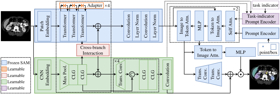
Figure 1: Overview of SAMCT. Modules painted in green, light red, and purple are the U-shaped CNN image encoder, the cross-branch interaction module, and the task-indicator prompt encoder respectively. All modules from SAM are painted in blue and frozen during training. CLG represents the combination of convolution, layer normalization, and Gelu. Trans.Conv. represents transpose convolution.

2.3 Prompts in SAMs

Accurate segmentation of SAMs relies on precise manual prompts, i.e., points, bounding boxes, or masks, which brings great inconvenience to its clinical deployment (He et al. 2023b). There are two ways to reduce the workload of SAMs. One way is to redesign the prompt encoders to generate prompt embeddings without human intervention. Auto-prompting SAM generates prompt embeddings from the image embedding by a down-up FCN subnetwork (Li et al. 2023a). SurgicalSAM develops a prototype-based prompt encoder to generate dense and sparse prompt embeddings (Yue et al. 2023). Despite their effectiveness, such prompt encoders are deeply coupled to the mask decoder, undermining the universality of SAM. The other way is to introduce additional object detectors or segmentation networks to obtain point or bounding box prompts. TongueSAM proposes a prompt generator based on object detection (Cao et al. 2023). UV-SAM produces mask and box prompts from the outputs of Segformer (Zhang et al. 2024). Similarly, AutoSAM uses a Harmonic Dense Net to generate prompt embeddings from input images (Shaharabany et al. 2023). Though these methods can protect the universality of the mask decoder, they need an additional heavy network to generate corresponding prompts for each downstream task, making the foundation model degenerate into a heavy ensemble model. Comparatively, SAMCT is equipped with an optional and lightweight task-indicator prompt encoder, which works as a plug-and-play component and is only related to target objects and independent of SAMCT itself.

3 Method

3.1 Overview

As depicted in Fig. 1, SAMCT is composed of the original SAM, a U-shaped CNN image encoder, a cross-branch interaction module, and an optional task-indicator prompt encoder. All parameters of SAM are frozen during training. To align the encoded feature space in SAM with medical imaging, we parallelize a simple adapter on the feed-forward layer of each transformer in the ViT image encoder of SAM. The adapter consists of a linear projection with $4\times$ channel decrease, a Gelu activation function, and a linear projection with $4\times$ channel increase. The U-shaped CNN image encoder, a branch placed in parallel with the ViT image encoder of SAM, is introduced to capture local features in high-resolution feature maps. Between them, the cross-branch interaction module is developed to transfer local information and global perception from one to the other. The encoded feature embeddings, together with the encoded prompt embeddings from the prompt encoder of SAM, flow into the mask decoder for final segmentation. In terms of the mask decoder, we fuse the full-resolution image features from CNN and the up-sampled ViT image embeddings before computing the final mask by dot product for further local feature enhancement. Combining with SAM, the U-shaped CNN image encoder and the cross-branch interaction module adapt SAM for segmenting any CT. Furthermore, to ease the usage of SAMCT in clinical scenarios, we propose a plug-and-play task-indicator prompt encoder to replace the manual prompt encoder and automatically produce effective prompt embeddings for each specific task.

3.2 U-shaped CNN Image Encoder

The design of the CNN image encoder is inspired by U-Net (Ronneberger, Fischer, and Brox 2015), which is proven to be more consistent with the characteristics of medical imaging as illustrated in Fig. 1. Given any input $x\in\mathbb{R}^{3\times H\times W}$, the HAAM module proposed by AAU-net (Chen et al. 2022) is first used to extract its CNN embedding $F_{c}\in\mathbb{R}^{d_{c}\times H\times W}$. Then, four encoding blocks are executed in sequence to continuously adjust its resolution and obtain deeper semantic features. Each encoding block consists of a max pooling, two sequential convolutions with the stride of 1 and the kernel size of 3$\times$3, a layer normalization, and a Gelu activation. Besides, the previous convolution doubles the input channels while the second convolution maintains its input channels. After such encoding blocks, we obtain the smallest feature map $F_{16}\in\mathbb{R}^{16d_{c}\times\frac{H}{16}\times\frac{W}{16}}$ of the CNN-branch. Then, four decoding blocks are executed sequentially to recover the resolution and capture important local features. Each decoding block starts with a transpose convolution with half the number of channels, a stride of 2, and a kernel size of 2. Then, the output of transpose convolution is concatenated with the same-resolution feature map from the encoding block through skip connection. After concatenation, two sequential convolutions, a layer normalization, and a Gelu activation are applied. During decoding, another four feature maps with different resolutions $F_{32}\in\mathbb{R}^{8d_{c}\times\frac{H}{8}\times\frac{W}{8}},F_{64}\in\mathbb{R}^{4d_{c}\times\frac{H}{4}\times\frac{W}{4}},F_{128}\in\mathbb{R}^{2d_{c}\times\frac{H}{2}\times\frac{W}{2}},F_{256}\in\mathbb{R}^{d_{c}\times H\times W}$ are generated. Finally, a $1\times 1$ convolution is to adjust the channel number to 32 to match that of the full-resolution image embedding in the mask decoder.

3.3 Cross-branch Interaction

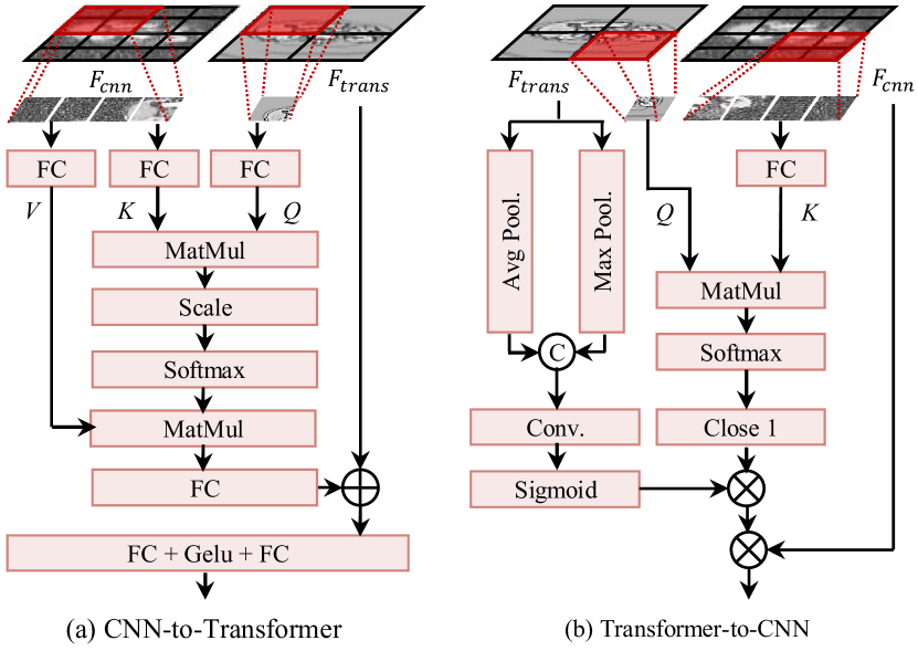
Figure 2: Two flows of the cross-branch interaction module.

Cross-branch interaction module builds two information flows between the ViT image encoder and the CNN image encoder, including the CNN-to-Transformer flow and the Transformer-to-CNN flow as depicted in Fig. 2. The inputs of cross-branch interaction include an image embedding $F_{cnn}$ from a certain scale of the CNN branch and an image embedding $F_{trans}$ from the ViT branch correspondingly. After aligning $F_{cnn}$ and $F_{trans}$, each patch $F_{p}\in\mathbb{R}^{1\times d_{p}}$ in $F_{trans}$ correspond to a $k\times k$ window $F_{w}\in\mathbb{R}^{k^{2}\times d_{w}}$ in $F_{cnn}$ as shown in the red regions of Fig. 2. In the CNN-to-Transformer flow, through three different projections, each patch $F_{p}$ can be recognized as a query (i.e., $Q$) and the corresponding $k\times k$ region $F_{w}$ can be recognized as key (i.e., $K$) and value (i.e., $V$) to build dependency via cross-attention, formulated as:

$$F_{c}=\text{{Softmax}}(\frac{F_{p}E_{q}(F_{w}E_{k})^{T}}{\sqrt{d_{p}}})(F_{w}E_{v}),$$ (1)

where $E_{k},E_{v}\in\mathbb{R}^{d_{w}\times d_{p}}$, and $E_{q}\in\mathbb{R}^{d_{p}\times d_{p}}$ are projection matrices. By combining $F_{p}$ with $F_{c}$ after projection, detailed/local features can flow from the CNN branch to the ViT branch.

In the Transformer-to-CNN flow, $F_{trans}$ can remind $F_{cnn}$ of regions demanding more attention across the entire image space based on its superior global perception. Therefore, we generate a spatial attention map to augment $F_{cnn}$ by a coarse-to-fine attention mechanism. First, we apply max pooling and average pooling onto $F_{trans}$ to generate a rough spatial attention map, where each pixel corresponds to a $k\times k$ window of $F_{cnn}$. To refine the attention in each $k\times k$ window of $F_{cnn}$, we compute the correlation between the patch $F_{p}$ and the corresponding window $F_{w}$ and normalize the value to (0.5, 1.5), formulated as:

$$A_{w}=\text{{Softmax}}(\frac{F_{p}(F_{w}E_{w})^{T}}{\sqrt{d_{p}}}),$$ (2)

$$A^{*}_{w}=\frac{e^{A_{w}-k^{-2}}}{1+e^{A_{w}-k^{-2}}}+0.5,$$

where $E_{w}\in\mathbb{R}^{d_{w}\times d_{p}}$ is a projection matrix to unify the dimensions of $F_{p}$ and $F_{w}$. After broadcasting the coarse attention $A_{p}\in\mathbb{R}^{1\times 1}$ of $F_{p}$ into $A^{*}_{p}\in\mathbb{R}^{k\times k}$, $A^{*}_{w}$ is multiplied by $A^{*}_{p}$ to obtain the refined attention map of $F_{w}$. Finally, multiplying the entire refined attention map with $F_{cnn}$ can supplement global information from the ViT branch to the CNN branch.

3.4 Task-indicator Prompt Encoder

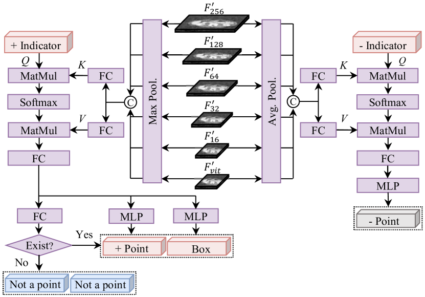
Figure 3: Details of the task-indicator prompt encoder.

Table 2: Composition of CT5M. Datasets with ^∗ are invisible during training and are only used for generalization verification.

Dataset	image	mask	Dataset	image	mask	Dataset	image	mask
HE-BCT∗ (Hssayeni et al. 2020)	1,070	316	LCTSC∗ (Yang et al. 2017)	14,338	38,342	DZ Task07 (Antonelli et al. 2022)	26,719	11,320
INSTANCE (Li et al. 2023b)	2,981	892	COVID-19 Seg∗ (Igor.Slinko 2020)	929	699	CHAOS (Kavur et al. 2021)	2,874	2,341
HaN-Seg (Podobnik et al. 2023)	7,581	24,990	LNDB (Pedrosa et al. 2019)	63,068	2,369	DZ Task09 (Antonelli et al. 2022)	3,650	1,050
Totalsegmentator (Wasserthal et al. 2023)	312,400	3,837,723	ATM∗ (Zhang et al. 2023)	190,724	124,231	KiTS23 (Heller et al. 2023)	95,221	16,826
HaN-OAR (Li and Chen 2020)	6,151	13,356	Pe-CT-SEG (Jordan et al. 2021)	110,083	618,599	DZ Task10 (Antonelli et al. 2022)	13,486	1,280
PDDCA∗ (Raudaschl et al. 2017)	7,367	6,053	DZ Task08 (Antonelli et al. 2022)	21,120	12,852	NIH-Pancreas (Roth et al. 2016)	18,942	6,881
COVID-19-20 (Roth et al. 2022)	13,705	4,956	AMOS22 (Ji et al. 2022)	41,430	129,237	COVID-19 Scan∗ (Ma et al. 2021)	3,520	1,844
MosMed (Morozov et al. 2020)	2,049	785	WORD (Luo et al. 2022)	24,218	59,192	A-ACC-Ki67 (Moawad et al. 2023)	6,008	1,400
MM-WHS∗ (Zhuang et al. 2019)	5,305	17,311	BTCV∗ (Landman et al. 2015)	3,779	12,175	FUMPE (Masoudi et al. 2018)	8,792	2,304
DZ Task06 (Antonelli et al. 2022)	17,657	1,646	LiTS (Bilic et al. 2023)	58,638	26,269	Pr-An-Ed-Ca∗ (Thompson et al. 2023)	23,359	23,191

The task-indicator prompt encoder takes task-specific positive and negative indicators, multi-resolution image embeddings from the CNN image encoder (i.e., $F_{16}$, $F_{32}$, $F_{64}$, $F_{128}$, and $F_{256}$), and the final image embedding $F_{vit}$ from the ViT image encoder as inputs to replace the manual prompt encoder in SAM and effortlessly generate positive point prompt embeddings, bounding box prompt embeddings, and negative point embeddings, as depicted in Fig. 3. First, we pre-process the inputs to map their features to the feature space of interest for the indicator-specific task. Specifically, image embeddings are projected into the task-specific feature space via linear projections, forming a series of new image embeddings $\{F^{\prime}\}=\{F^{\prime}_{16}$, $F^{\prime}_{32}$, $F^{\prime}_{64}$, $F^{\prime}_{128}$, $F^{\prime}_{256}$, $F^{\prime}_{vit}$}. For a given task, a positive task-related indicator $P^{+}\in\mathbb{R}^{1\times d_{p}}$ and a negative task-related indicator $P^{-}\in\mathbb{R}^{1\times d_{p}}$ are learned to generate the corresponding prompt embeddings. In each image embedding, as the maximum value usually reflects the most representative region for the given task (i.e., foreground) and the average value usually corresponds to background, we apply both max pooling and average pooling onto $\{F^{\prime}\}$ and concatenate them to generate the positive image embedding $F^{+}$ and the negative image embedding $F^{-}$ respectively. Then, the negative point embedding ${Pe}^{-}$ is obtained by calculating cross-attention between $P^{-}$ and $F^{-}$, formulated as:

$$A^{-}=\text{{Softmax}}(\frac{P^{-}E_{q^{-}}(F^{-}E_{k^{-}})^{T}}{\sqrt{d_{p}}}),$$ (3)

$${Pe}^{-}=\text{{Gelu}}((A^{-}(F^{-}E_{v^{-}}))E_{-}E_{1})E_{2},$$

where $E_{q^{-}},E_{k^{-}},E_{v^{-}},E_{-},E_{1}$, and $E_{2}$ are projection matrices. Following Eq. 3, we can calculate $A^{+}$, the positive point embedding $Pe^{+}$, and the positive bounding box embedding $Be^{+}$. It is noted that not all inputs have foreground and providing positive prompts may be counter-productive. To address this, a classifier is added to the positive flow, formulated as

$$p=\text{{Softmax}}(A^{+}(F^{+}E_{v^{+}})E_{+}E_{c}),$$ (4)

where $E_{c}\in\mathbb{R}^{d_{p}\times 2}$ is a classification matrix. When $p$ indicates no foreground existing, the not-a-point embedding $Ne$ is used instead of the $Pe^{+}$ and $Be^{+}$ to prompt the mask decoder. $Ne$ is from the original SAM and frozen during training.

3.5 Training Strategies

Parameters of the shared parts between SAMCT and SAM inherit from SAM trained on SA-1B (Kirillov et al. 2023). During training SAMCT, only newly introduced parameters are updated through the standard Dice and binary cross-entropy losses. When training the task-indicator prompt encoder for any specific task, an additional cross-entropy loss is adopted to penalize $p$. When foreground exists, the prompts during training contain a randomly sampled positive point, a randomly sampled negative point, and a randomly shifted bounding box. Otherwise, the prompts only contain two randomly sampled negative points. For image-mask pairs converted from 3D data, as there exist many full background pairs, during most training rounds, we randomly select $10\%$ ($\leq$1000 pairs) of them for each object. The performance of SAMCT is evaluated under the prompts of a center positive point and a bounding box.

Table 3: Object Mapping. H: Head and Neck, C: Chest, A: Abdomen, P: Pelvis, B:Bone, L: lesion, V: vessel.

Object	ID	Object	ID	Object	ID	Object	ID
brainstem	H1	left submandibular gland	H2	right submandibular gland	H3	optic chiasm	H4
left optic nerve	H5	right optic nerve	H6	left parotid gland	H7	right parotid gland	H8
spinal cord	H9	esophagus	H10	brain	H11	buccal mucosa	H12
oral cavity	H13	anterior segment (left eyeball)	H14	anterior segment (right eyeball)	H15	posterior segment (left eyeball)	H16
posterior segment (right eyeball)	H17	left lacrimal gland	H18	right lacrimal gland	H19	lips	H20
pituitary gland	H21	face	H22	left eye	H23	right eye	H24
left lens	H25	right lens	H26	left temporal lobes	H27	right temporal lobes	H28
left inner ear	H29	right inner ear	H30	left middle ear	H31	right middle ear	H32
cricopharyngeal inlet	H33	thyroid	H34	larynx-glottis	H35	larynx-supraglottic	H36
left ventricle	C1	right ventricle	C2	left atrium	C3	right atrium	C4
myocardium	C5	right lung	C6	left lung	C7	trachea	C8
body	C9	left breast	C10	right breast	C11	thymus	C12
pancreas	A1	spleen	A2	right kidney	A3	left kidney	A4
gallbladder	A5	liver	A6	stomach	A7	right adrenal gland	A8
left adrenal gland	A9	bladder	A10	prostate	A11	rectum	A12
duodenum	A13	colon	A14	large Intestine	A15	large Intestine	A16
gonads	A17	skin	A18	left autochthon	A19	right autochthon	A20
utero cervix	P1	left gluteus maximus	P2	right gluteus maximus	P3	left gluteus medius	P4
right gluteus medius	P5	left gluteus minimus	P6	right gluteus minimus	P7	left iliopsoas	P8
right iliopsoas	P9	mandible	B1	left head of femur	B2	right head of femur	B3
temporomandibular joint (left)	B4	temporomandibular joint (right)	B5	arytenoid	B6	left clavicula	B7
right clavicula	B8	left humerus	B9	right humerus	B10	left rib	B11
right rib	B12	left scapula	B13	right scapula	B14	vertebrae	B15
spinal canal	B16	left hip	B17	right hip	B18	sacrum	B19
hemorrhage	L1	COVID-19	L2	lung tumor	L3	pancreas tumor	L4
colon cancer	L5	pulmonary embolism	L6	pulmonary nodule	L7	liver tumor	L8
kidney tumor	L9	cyst	L10	adrenocortical carcinoma	L11	aorta	V1
pulmonary artery	V2	inferior vena cava	V3	portal and splenic vein	V4	left carotid artery	V5
right carotid artery	V6	hepatic vessel	V7	left iliac artery	V8	right iliac artery	V9
left iliac vena	V10	right iliac vena	V11

4 Experiments

In this section, CT5M is first described in Sec. 4.1. The versatility and generalization of SAMCT trained on CT5M are evaluated on 30 datasets across 118 objects in Sec. 4.2. Then, SAMCT is compared against both foundation models in Sec. 4.3 and SOTA specific models in Sec. 4.4. Component-wise ablation study of SAMCT are presented in Sec. 4.5. Finally, the effectiveness of the task-indicator prompt encoder is verified in Sec. 4.6.

4.1 Dataset: CT5M

CT5M is collected from 30 publicly available datasets as summarized in Table 2. As both annotation protocols and data formats of datasets are different, a series of preprocessing operations are adopted to standardize the collected public datasets. For 2D data, all data is converted to the .PNG format for consistent data loading. For volumetric data, all 3D data is converted to 2D slices across the coronal plane to match the inputs of SAM-based models. As the intensity range of CT is usually (-1024, 2048), directly compressing such a large range to (0, 255) may lose valuable information. Therefore, under the guidance of experts, we choose different density windows for objects. Specifically, the intensity ranges of bone, tissue, lung, and hemorrhage are set as (-400, 1100), (-200, 300), (-1300, 300), and (-20, 100) respectively.

The collection of masks/objects has been carefully screened and checked to ensure that data is not duplicated and annotation rules are consistent. For instance, the adrenal glands are labeled as left and right adrenal glands in the AMOS dataset, while they are labeled as a whole in the WORD dataset. At this point, we only retain the fine left and right adrenal gland masks to remove annotation ambiguity. After the above preprocessing, CT5M collects 5M masks with foreground regions from 1.1M images of 30 publicly available datasets.

According to the scanning position and object attribute, we divide objects in CT5M into seven categories, including head and neck (H), chest (C), abdomen (A), pelvis (P), lesion (L), bone (B), and vessel (V). Totally 118 objects from the above seven categories are included in CT5M. Details of objects and their mapping abbreviations are summarized in Table 3.

To conduct plentiful generalization and versatility verification, nine out of the preprocessed 30 datasets (i.e., datasets marked with $*$ in Table 2) were set as training invisible, and the rest were selected as training visible. For training invisible datasets, all data is used as the testing set to evaluate the generalization ability of SAMCT. As for each training visible dataset, data is divided into training, validation, and testing sets. The segmentation performance of SAMCT on such visible testing sets reflects its versatility. Data partitioning of training visible datasets follows publicly available data splits. For datasets without public data partitioning or with only training set labels, they are randomly divided into training, validation, and testing sets in a 7:1:2 ratio. For datasets with only training and validation set labels, the validation set is divided into validation and testing sets in a 1:1 ratio.

4.2 Versatility and Generalization on CT5M

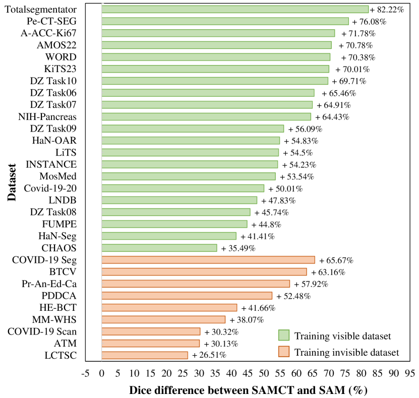
Figure 4: Comparison between SAMCT and SAM across 21 training visible datasets (versatility) and 9 training invisible datasets (generalization). SAMCT consistently outperforms SAM with large margins.

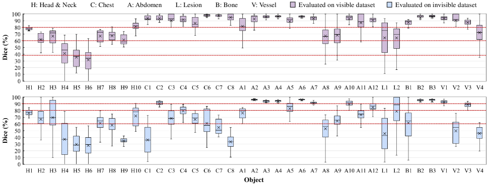
Figure 5: Dice boxplot of SAMCT on visible and invisible datasets across 39 objects. Objects are represented by groups of category letters and ID numbers, and the object mapping table is provided in Table  3.

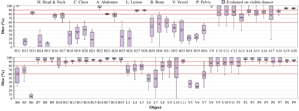
Figure 6: Dice boxplot of SAMCT on visible datasets across the rest 79 objects. Objects are represented by groups of category letters and ID numbers, and the object mapping table is provided in Table  3.

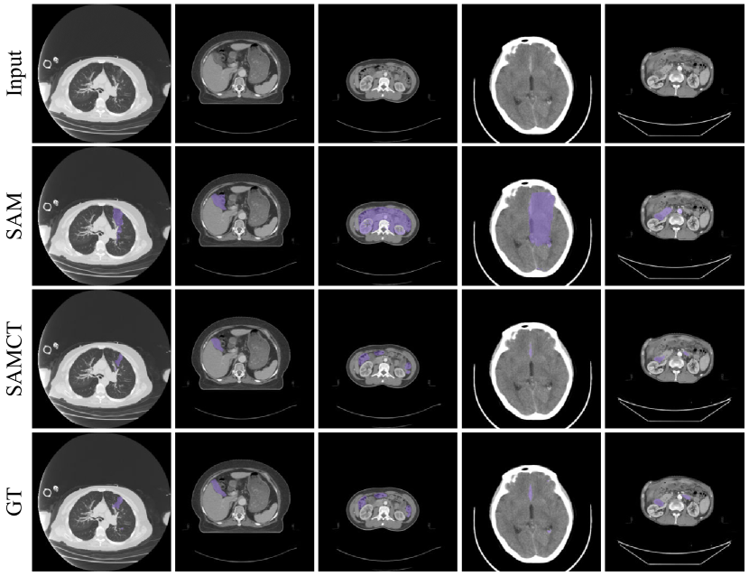
Figure 7: Qualitative comparisons between SAM and SAMCT across 5 different objects. GT represents the ground truth.

Setting. To train a powerful CT foundation model for auxiliary annotation and clinical applications, we trained SAMCT on the complete training data of CT5M and evaluated its versatility and generalization. During training, prompts were randomly sampled from positive points, negative points, and shifted bounding boxes generated from the masks. SAMCT was trained by an Adam optimizer with an initial learning rate of 0.0006 and a batch size of 48 for 50 epochs where the learning rate is adjusted to 0.0001 on the 10th epoch. Random rotation, random scaling, cropping, contrast adjustment, and gamma augmentation were applied for data augmentation.

Table 4: Dice comparison of foundation models on three representative training visible datasets, including COVID-19-20 (Roth et al. 2022), INSTANCE (Li et al. 2023b), and WORD (Luo et al. 2022), covering 16 objects. Note: ICH: intracranial hemorrhage, Liv: liver, Spl: spleen, LKid: left kidney, RKid: right kidney, Sto: stomach, Gall: gallbladder, Eso: esophagus, Pan: pancreas, Dou: duodenum, Col: colon, Rec: rectum, B: bladder, LHF: left head of femur, RHF: left head of femur, and Avg: the average Dice across 16 objects.

Method	COVID-19	ICH	Liv	Spl	Lkid	Rkid	Sto	Gal	Eso	Pan	Duo	Col	Rec	Bla	LHF	RHF	Avg
SAM (Kirillov et al. 2023)	15.55	10.26	41.88	22.55	20.00	19.62	22.76	2.02	1.66	6.87	5.69	16.66	10.39	17.85	24.06	23.93	16.36
SAM-Med2D (Cheng et al. 2023)	69.69	73.11	95.24	94.16	94.12	94.26	92.14	78.14	78.88	80.94	73.15	79.76	89.27	94.27	94.35	94.33	85.99
MedSAM (Ma and Wang 2023)	67.65	69.36	94.59	95.51	95.25	95.45	93.23	84.99	81.84	82.94	78.38	80.92	89.09	94.74	95.05	94.38	87.09
SAMed (Zhang and Liu 2023)	77.33	74.36	95.24	93.68	93.52	92.82	92.92	83.18	82.07	84.63	79.57	83.34	90.43	94.07	94.03	93.42	87.79
MSA (Wu et al. 2023)	76.54	77.58	96.04	95.33	95.19	95.23	93.57	83.75	83.74	84.59	79.72	85.35	91.54	94.89	95.29	95.42	88.99
SAMCT	77.59	77.66	96.35	95.86	95.61	95.82	93.99	83.87	85.03	86.02	82.14	86.29	91.29	95.33	95.85	96.09	89.67

Quantitative Results. Comparison between SAMCT and SAM is depicted in Fig. 4. Any bar in green has a positive value in Fig. 4 indicates that SAMCT outperforms SAM when tested on a training visible dataset, where CHAOS (Kavur et al. 2021) is of the least performance improvements among training visible datasets, with an average increase of $35.49\%$ in Dice and Totalsegmentator (Wasserthal et al. 2023) is of the most performance improvements with an average increase of $82.22\%$ in Dice. It demonstrates the brilliant versatility of SAMCT on various downstream tasks. As for the generalization performance of SAMCT, all training invisible datasets own noticeable performance improvements, where LCTSC (Yang et al. 2017) is of the least improvements with an average increase of $26.51\%$ in Dice and COVID-19 Seg (Igor.Slinko 2020) is of the most performance improvements with an average increase of $65.67\%$ in Dice. It proves the prominent generalization ability of SAMCT.

To analyze the object-specific performance of SAMCT, we calculate and plot the average Dice score of each object in Figs. 5 and 6. For training visible datasets, most objects in chest, abdomen, bone, and pelvis have an average Dice score greater than $90\%$. Specifically, 44 out of 118 objects have an average Dice score greater than 90$\%$ and 68 out of 118 objects have an average Dice score greater than $80\%$, validating the surprising versatility of SAMCT. Among 4,236,340 training image-mask pairs, the numbers of masks for H4, H5, H6, H12, H14, and H15 are only 146, 235, 241, 448, 186, and 201, respectively, resulting in relatively poor performance of SAMCT. Similarly, B5 and some other objects in head and neck exhibit poorer performance due to relatively limited training data. For training invisible datasets, 16 and 10 out of 39 objects have an average Dice score greater than $80\%$ and $90\%$, making SAMCT a powerful tool for clinically-assisted annotation.

Qualitative Results. Qualitative segmentation results of SAM and SAMCT are illustrated in Fig. 7. Visually, segmenting various medical objects via one model is challenging, especially for those with low contrast, blurry boundaries, small sizes, and complex shapes. Compared to SAM, SAMCT can accurately identify such hard objects, validating the effectiveness of constructing the large CT dataset (i.e., CT5M), the U-shaped CNN image encoder, and the cross-branch interaction in SAMCT.

4.3 Comparison with Foundation Models

Setting. Experiments are conducted on a subset of CT5M, consisting of COVID-19-20 (Roth et al. 2022), INSTANCE (Li et al. 2023b), and WORD (Luo et al. 2022) and covering 16 objects. For a fair comparison, all models are initialized with SAM and prompted by the joint of random point and random box prompts in training. During inference, all models generate masks under the prompt of the joint center point and bounding box. All models were trained by an Adam optimizer with an initial learning rate of $1e^{-4}$ and a batch size of 8. A separate BTCV (Landman et al. 2015) dataset with overlapping objects of WORD, i.e., liver, spleen, left kidney, right kidney, stomach, gallbladder, esophagus, and pancreas, are used for generalization verification.

Results. Quantitative comparison results of different foundation models on three representative training visible datasets are summarized in Table 4. Among SAM-based models for medicine, all models can greatly improve the performance of SAM by learning more medical knowledge, where MedSAM (Ma and Wang 2023) and MSA (Wu et al. 2023) achieve the best performance in gallbladder and rectum segmentation, respectively. Besides, MSA achieves the best average Dice across 16 objects among comparison models. Comparatively, SAMCT achieves the second-best performance in the segmentation of gallbladder and rectum and outperforms all comparison models on the other 14 objects, leading to the best average Dice score of $89.67\%$. Quantitative comparison results of different foundation models on the training invisible BTCV (Landman et al. 2015) dataset are summarized in Table 5. SAM-based medical models are still much superior compared to SAM on generalization, especially for small-size objects, e.g., gallbladder and esophagus, and low-contrast objects, e.g., stomach. Specifically, MSA and MedSAM achieve the best performance in segmenting esophagus and right kidney, with the Dice scores of $84.15\%$ and $90.69\%$, respectively. Compared to MSA and MedSAM, though SAMCT performs slightly worse on esophagus and right kidney, it is superior on the other 6 objects, leading to an improvement of $5.06\%$ and $1.75\%$ in average Dice across 8 objects. It should be noted that the best comparison models for training visible and invisible validation are different (i.e., MSA and MedSAM respectively) while SAMCT consistently achieves the best overall performance, demonstrating the brilliant versatility and generalization ability of SAMCT.

4.4 Comparison with Task-Specific Models

Setting. Comparison models include SAMCT trained on a subset of CT5M (denoted as SAMCT-Sub obtained in Sec. 4.3), SAMCT trained on CT5M (denoted as SAMCT-CT5M obtained in Sec. 4.2), and 13 SOTA task-specific models. Task-specific models consist of four 2D CNN-based methods, i.e., U-Net (Ronneberger, Fischer, and Brox 2015), CPFNet (Feng et al. 2020), CA-Net (Gu et al. 2020), and AAU-net (Chen et al. 2022), four 2D transformer-based methods, i.e., TransFuse (Zhang, Liu, and Hu 2021), TransUNet (Chen et al. 2021), MISSFormer (Huang et al. 2022), and H2Former (He et al. 2023a), and five 3D methods, i.e., nnU-Net (Isensee et al. 2021), SwinUNETR (Hatamizadeh et al. 2021), UNETR (Hatamizadeh et al. 2022), nnFormer (Zhou et al. 2023), and MedNeXt (Roy et al. 2023). All task-specific models were trained on INSTANCE (Li et al. 2023b) and WORD (Luo et al. 2022) respectively following the same settings with SAMCT.

Table 5: Dice comparison of foundation models on the training invisible BTCV (Landman et al. 2015) dataset.

Method	Liv	Spl	Lkid	Rkid	Sto	Gal	Eso	Pan	Avg
SAM (Kirillov et al. 2023)	56.51	30.05	27.34	27.96	28.34	4.01	2.54	32.99	26.22
SAM-Med2D (Cheng et al. 2023)	83.54	91.60	90.10	90.22	75.57	76.47	82.74	57.39	80.95
MSA (Wu et al. 2023)	81.90	92.79	89.74	89.58	80.39	70.77	84.15	60.75	81.26
SAMed (Zhang and Liu 2023)	81.73	91.85	87.37	88.33	80.57	77.67	80.57	66.42	81.81
MedSAM (Ma and Wang 2023)	88.33	90.44	90.52	90.69	81.29	83.48	84.06	67.73	84.57
SAMCT	89.98	95.29	90.98	90.56	85.23	84.15	83.74	70.63	86.32

Table 6: Comparison of SAMCT and SOTA task-specific models on the training visible INSTANCE (Li et al. 2023b) and WORD (Luo et al. 2022) datasets.

Method	INSTANCE			WORD
	Dice	HD	IoU	Dice	HD	IoU
U-Net (Ronneberger, Fischer, and Brox 2015)	51.91	22.75	44.03	86.53	17.04	78.47
CPFNet (Feng et al. 2020)	52.30	22.45	43.58	83.74	18.41	74.64
CA-Net (Gu et al. 2020)	55.07	22.30	45.29	85.86	17.35	77.59
AAU-net (Chen et al. 2022)	56.91	20.30	48.24	86.63	16.46	78.42
TransFuse (Chen et al. 2022)	44.42	24.40	35.54	74.39	20.87	62.44
TransUnet (Chen et al. 2021)	51.75	22.10	43.42	85.38	17.37	76.84
MISSFormer (Huang et al. 2022)	58.18	21.35	48.26	84.16	17.99	75.16
H2Former (He et al. 2023a)	58.22	19.70	48.83	85.79	17.82	77.31
SwinUNETR (Hatamizadeh et al. 2021)	60.00	18.85	49.99	73.23	14.29	62.66
nnFormer (Zhou et al. 2023)	60.61	18.45	50.76	78.94	13.73	67.55
UNETR (Hatamizadeh et al. 2022)	60.97	18.75	50.81	75.27	13.63	65.38
nnU-Net (Isensee et al. 2021)	63.18	18.45	52.91	84.52	12.09	75.27
MedNeXt (Roy et al. 2023)	64.14	18.05	53.80	83.73	12.77	74.06
SAMCT-Sub	77.66	15.90	65.76	91.40	12.29	84.73
SAMCT-CT5M	64.49	19.45	52.88	87.23	4.33	87.57

Table 7: Dice comparison of SAMCT and SOTA specific models on the training invisible BTCV (Landman et al. 2015) dataset.

Method	Liv	Spl	Lkid	Rkid	Sto	Gal	Eso	Pan	Avg
CPFNet (Feng et al. 2020)	64.25	4.96	3.13	1.34	24.75	0.00	6.24	0.00	13.08
U-Net (Ronneberger, Fischer, and Brox 2015)	77.22	19.46	22.80	15.80	12.89	3.52	7.92	1.50	20.14
CA-Net (Gu et al. 2020)	70.77	28.18	10.82	16.04	23.46	0.54	31.02	3.42	23.03
AAU-net (Chen et al. 2022)	78.18	30.96	29.60	32.18	19.61	0.14	25.29	1.50	27.18
TransUNet (Chen et al. 2021)	68.67	9.46	1.71	0.74	19.08	3.58	2.43	1.60	13.41
TransFuse (Zhang, Liu, and Hu 2021)	77.13	4.04	4.73	3.76	14.55	3.33	0.40	0.01	13.49
MISSFormer (Huang et al. 2022)	65.45	21.74	8.75	2.99	15.35	3.68	9.26	2.68	16.24
H2Former (He et al. 2023a)	77.34	21.57	0.84	2.47	36.95	0.15	13.28	4.32	19.62
SwinUNETR (Hatamizadeh et al. 2021)	84.24	68.03	69.36	74.58	54.11	32.29	38.19	30.44	56.41
nnFormer (Zhou et al. 2023)	85.16	72.20	69.89	75.76	54.60	44.08	44.04	33.59	59.91
UNETR (Hatamizadeh et al. 2022)	84.49	66.32	71.66	76.83	55.22	30.32	36.60	32.98	56.80
nnU-Net (Isensee et al. 2021)	91.03	78.55	84.93	85.87	67.63	59.89	75.09	54.09	74.64
MedNeXt (Roy et al. 2023)	90.09	82.35	79.26	80.34	63.58	55.91	67.96	47.73	70.90
SAMCT-Sub	89.98	95.29	90.98	90.56	85.23	84.15	83.74	70.63	86.32
SAMCT-CT5M	96.33	96.13	93.38	93.13	91.14	82.99	82.72	91.42	90.91

Results. Quantitative comparison results of different methods on visible INSTANCE (Li et al. 2023b) and WORD (Luo et al. 2022) are summarized in Table 6. Among task-specific methods, MedNeXt (Roy et al. 2023) achieves the best performance on INSTANCE and nnU-Net (Isensee et al. 2021) achieves the best performance on WORD. Comparatively, SAMCT trained on either partial or complete CT5M achieves better performance than all task-specific methods across the two datasets. Quantitative comparison results of different methods on the invisible BTCV (Landman et al. 2015) dataset are summarized in Table 7. Obviously, task-specific methods perform poorly on invisible data due to domain shift. Comparatively, the performance of SAMCT is much better, with average Dice scores of $86.32\%$ and $90.91\%$ by SAMCT-Sub and SAMCT-CT5M, respectively. Benefiting from the construction of CT5M, though SAMCT-CT5M performs slightly worse in visible datasets due to the lower proportion of training targets compared to SAMCT-Sub, its performance on invisible datasets is much greater than that of SAMCT-Sub.

Table 8: Component-wise ablation study of SAMCT on the COVID-19-20 (Roth et al. 2022) dataset. CNN, CBI, and Adapter represent the U-shaped CNN image encoder, cross-branch interaction, and adapters in the ViT image encoder.

CNN	CBI	Adapter	Dice	HD	IOU
$\bullet$	$\bullet$	$\bullet$	76.20	27.56	62.43
$\bullet$	$\bullet$	$\circ$	75.35	28.28	61.39
$\bullet$	$\circ$	$\bullet$	75.63	26.03	61.62
$\circ$	$\circ$	$\bullet$	74.90	31.23	61.21

4.5 Component-Wise Ablation Study

Component-wise ablation study of SAMCT is summarized in Table 8. Generally, removing any component is harmful, validating the effective designs of SAMCT.

4.6 Comparison with Various Prompt Modes

Setting. We conduct a comparison between task-indicator prompt and various manual prompts, including the randomly sampled point prompt, the center point prompt, the random box prompt with an offset of less than $5\%$ width/height, the bounding box prompt, and the joint center point and bounding box prompt. SAMCT-CT5M is evaluated on WORD (Luo et al. 2022) under the above prompts. The task-indicator prompt encoder is a plug-in module independent of SAMCT and trained on the frozen SAMCT-CT5M with an initial learning rate of 0.0003 and a batch size of 12.

Results. Quantitative comparison under various prompts is summarized in Table 9. In terms of the random point prompt and the center point prompt, the former achieves better results in segmenting liver, spleen, and left kidney while the latter is better on segmenting right kidney, left head of femur, and right head of femur. In other words, the position of point prompts has a crucial impact on the performance of SAM-based methods, and no point type has been proven to be the best for all. In contrast, the segmentation results generated under different box prompts are relatively stable and better than various point prompts. Besides, using the joint center point and bounding box prompt consistently achieves the best performance among manual prompt modes. Comparatively, the proposed task-indicator prompt consistently outperforms any point prompt, achieving better performance than the random box prompt in segmenting liver, left kidney, right kidney, and left head of femur, approaching the best manual prompt in segmenting liver, spleen, left head of femur, and right head of femur, and even outperforming the best manual prompt in segmenting left kidney and right kidney. Though the task-indicator prompt cannot completely surpass the best manual prompt, it is labor-free and more easy-to-use in clinical applications. In addition, as a plug-and-play module, it is very lightweight with only 1.7M parameters, being highly extendable to other foundation models.

Table 9: Dice comparison of different prompts on objects from the WORD dataset. Cpoint+bbox represents using the joint center point and bounding box prompt.

Prompt Mode	Liv	Spl	Lkid	Rkid	LHF	RHF
random ponit	90.18	93.82	93.50	91.40	90.11	91.54
center point	86.71	93.6	92.77	93.60	90.69	91.94
random box	95.27	94.57	93.62	93.66	92.90	93.66
bounding box	95.46	94.67	93.77	93.90	93.05	93.72
cpoint+bbox	95.49	94.82	94.23	94.22	93.77	93.98
task-indicator	95.30	94.03	94.29	94.50	92.96	92.99

5 Conclusion

In this work, we present a large CT image dataset and a novel segmentation foundation model named SAMCT for various CT-related segmentation tasks. Different from existing research on tuning SAM on medical data, SAMCT has three unique components, including a U-shaped CNN image encoder for local feature supplement, a cross-branch interaction module for knowledge transfer, and a task-indicator prompt encoder for labor-free interaction. It deserves mentioning that the task-indicator prompt provides a new paradigm for labor-free prompts, converting semi-automatic interaction in SAM into fully-automatic interaction in SAMCT, which is more convenient and favorable in clinical applications. Extensive comparison experiments demonstrate the extraordinary versatility and generalization ability of SAMCT, outperforming SOTA both medical foundation models and task-specific models on various tasks, even without manual prompts.

References

- Antonelli et al. (2022) Antonelli, M.; Reinke, A.; Bakas, S.; Farahani, K.; Kopp-Schneider, A.; Landman, B. A.; Litjens, G.; Menze, B.; Ronneberger, O.; Summers, R. M.; et al. 2022. The medical segmentation decathlon. Nature Communications, 13(1): 4128.
- Bilic et al. (2023) Bilic, P.; Christ, P.; Li, H. B.; Vorontsov, E.; Ben-Cohen, A.; Kaissis, G.; Szeskin, A.; Jacobs, C.; Mamani, G. E. H.; Chartrand, G.; et al. 2023. The liver tumor segmentation benchmark (LiTS). Medical Image Analysis, 84: 102680.
- Cao et al. (2023) Cao, S.; Ruan, Q.; Wu, Q.; and Zhang, Z. 2023. TongueSAM: An universal tongue segmentation model based on SAM with zero-shot. arXiv preprint arXiv:2308.06444.
- Chen et al. (2022) Chen, G.; Li, L.; Dai, Y.; Zhang, J.; and Yap, M. H. 2022. AAU-net: an adaptive attention U-net for breast lesions segmentation in ultrasound images. IEEE Transactions on Medical Imaging.
- Chen et al. (2021) Chen, J.; Lu, Y.; Yu, Q.; Luo, X.; Adeli, E.; Wang, Y.; Lu, L.; Yuille, A. L.; and Zhou, Y. 2021. Transunet: Transformers make strong encoders for medical image segmentation. arXiv preprint arXiv:2102.04306.
- Cheng et al. (2023) Cheng, J.; Ye, J.; Deng, Z.; Chen, J.; Li, T.; Wang, H.; Su, Y.; Huang, Z.; Chen, J.; Jiang, L.; et al. 2023. SAM-Med2D. arXiv preprint arXiv:2308.16184.
- Feng et al. (2020) Feng, S.; Zhao, H.; Shi, F.; Cheng, X.; Wang, M.; Ma, Y.; Xiang, D.; Zhu, W.; and Chen, X. 2020. CPFNet: Context pyramid fusion network for medical image segmentation. IEEE Transactions on Medical Imaging, 39(10): 3008–3018.
- Gu et al. (2020) Gu, R.; Wang, G.; Song, T.; Huang, R.; Aertsen, M.; Deprest, J.; Ourselin, S.; Vercauteren, T.; and Zhang, S. 2020. CA-Net: Comprehensive attention convolutional neural networks for explainable medical image segmentation. IEEE Transactions on Medical Imaging, 40(2): 699–711.
- Hatamizadeh et al. (2021) Hatamizadeh, A.; Nath, V.; Tang, Y.; Yang, D.; Roth, H. R.; and Xu, D. 2021. Swin unetr: Swin transformers for semantic segmentation of brain tumors in mri images. In International MICCAI Brainlesion Workshop, 272–284. Springer.
- Hatamizadeh et al. (2022) Hatamizadeh, A.; Tang, Y.; Nath, V.; Yang, D.; Myronenko, A.; Landman, B.; Roth, H. R.; and Xu, D. 2022. Unetr: Transformers for 3d medical image segmentation. In Proceedings of the IEEE/CVF Winter Conference on Applications of Computer Vision, 574–584.
- He et al. (2023a) He, A.; Wang, K.; Li, T.; Du, C.; Xia, S.; and Fu, H. 2023a. H2Former: An efficient hierarchical hybrid transformer for medical image segmentation. IEEE Transactions on Medical Imaging.
- He et al. (2023b) He, S.; Bao, R.; Li, J.; Grant, P. E.; and Ou, Y. 2023b. Accuracy of segment-anything model (sam) in medical image segmentation tasks. arXiv preprint arXiv:2304.09324.
- Heller et al. (2023) Heller, N.; Isensee, F.; Trofimova, D.; Tejpaul, R.; Zhao, Z.; Chen, H.; Wang, L.; Golts, A.; Khapun, D.; Shats, D.; et al. 2023. The KiTS21 challenge: Automatic segmentation of kidneys, renal tumors, and renal cysts in corticomedullary-phase CT. arXiv preprint arXiv:2307.01984.
- Hssayeni et al. (2020) Hssayeni, M. D.; Croock, M. S.; Salman, A. D.; Al-Khafaji, H. F.; Yahya, Z. A.; and Ghoraani, B. 2020. Computed tomography images for intracranial hemorrhage detection and segmentation. Intracranial Hemorrhage Segmentation Using A Deep Convolutional Model. Data, 5(1): 14.
- Huang et al. (2022) Huang, X.; Deng, Z.; Li, D.; Yuan, X.; and Fu, Y. 2022. Missformer: An effective transformer for 2d medical image segmentation. IEEE Transactions on Medical Imaging.
- Huang et al. (2023) Huang, Y.; Yang, X.; Liu, L.; Zhou, H.; Chang, A.; Zhou, X.; Chen, R.; Yu, J.; Chen, J.; Chen, C.; Chi, H.; Hu, X.; Fan, D.-P.; Dong, F.; and Ni, D. 2023. Segment anything model for medical images? arXiv preprint arXiv:2304.14660.
- Igor.Slinko (2020) Igor.Slinko. 2020. COVID-19 CT images segmentation.
- Isensee et al. (2021) Isensee, F.; Jaeger, P. F.; Kohl, S. A.; Petersen, J.; and Maier-Hein, K. H. 2021. nnU-Net: a self-configuring method for deep learning-based biomedical image segmentation. Nature Methods, 18(2): 203–211.
- Ji et al. (2022) Ji, Y.; Bai, H.; Yang, J.; Ge, C.; Zhu, Y.; Zhang, R.; Li, Z.; Zhang, L.; Ma, W.; Wan, X.; et al. 2022. AMOS: A large-scale abdominal multi-organ benchmark for versatile medical image segmentation. arXiv preprint arXiv:2206.08023.
- Jordan et al. (2021) Jordan, P.; Adamson, P. M.; Bhattbhatt, V.; Beriwal, S.; Shen, S.; Radermecker, O.; Bose, S.; Strain, L. S.; Offe, M.; Fraley, D.; et al. 2021. Pediatric chest/abdomen/pelvic CT exams with expert organ contours (Pediatric-CT-SEG).
- Kapoor, McCook, and Torok (2004) Kapoor, V.; McCook, B. M.; and Torok, F. S. 2004. An introduction to PET-CT imaging. Radiographics, 24(2): 523–543.
- Kavur et al. (2021) Kavur, A. E.; Gezer, N. S.; Barış, M.; Aslan, S.; Conze, P.-H.; Groza, V.; Pham, D. D.; Chatterjee, S.; Ernst, P.; Özkan, S.; et al. 2021. CHAOS challenge-combined (CT-MR) healthy abdominal organ segmentation. Medical Image Analysis, 69: 101950.
- Kirillov et al. (2023) Kirillov, A.; Mintun, E.; Ravi, N.; Mao, H.; Rolland, C.; Gustafson, L.; Xiao, T.; Whitehead, S.; Berg, A. C.; Lo, W.-Y. L.; Dollár, P.; and Girshick, R. 2023. Segment anything. arXiv preprint arXiv:2304.02643.
- Landman et al. (2015) Landman, B.; Xu, Z.; Igelsias, J.; Styner, M.; Langerak, T.; and Klein, A. 2015. MICCAI multi-atlas labeling beyond the cranial vault–workshop and challenge. In Proc. MICCAI Multi-Atlas Labeling Beyond Cranial Vault—Workshop Challenge, volume 5, 12.
- Li et al. (2023a) Li, C.; Khanduri, P.; Qiang, Y.; Sultan, R. I.; Chetty, I.; and Zhu, D. 2023a. Auto-prompting SAM for mobile friendly 3D medical image segmentation. arXiv preprint arXiv:2308.14936.
- Li and Chen (2020) Li, H.; and Chen, M. 2020. Automatic structure segmentation for radio therapy planning challenge 2020. In Proceedings of the International Conference on Medical Image Computing and Computer-Assisted Intervention, Lima, Peru, 4–8.
- Li et al. (2023b) Li, X.; Luo, G.; Wang, K.; Wang, H.; Li, S.; Liu, J.; Liang, X.; Jiang, J.; Song, Z.; Zheng, C.; et al. 2023b. The state-of-the-art 3D anisotropic intracranial hemorrhage segmentation on non-contrast head CT: The INSTANCE challenge. arXiv preprint arXiv:2301.03281.
- Li, Hu, and Yang (2023) Li, Y.; Hu, M.; and Yang, X. 2023. Polyp-sam: Transfer sam for polyp segmentation. arXiv preprint arXiv:2305.00293.
- Luo et al. (2022) Luo, X.; Liao, W.; Xiao, J.; Chen, J.; Song, T.; Zhang, X.; Li, K.; Metaxas, D. N.; Wang, G.; ; and Zhang, S. 2022. WORD: A large scale dataset, benchmark and clinical applicable study for abdominal organ segmentation from CT image. Medical Image Analysis, 82: 102642–102642.
- Ma and Wang (2023) Ma, J.; and Wang, B. 2023. Segment anything in medical images. arXiv preprint arXiv:2304.12306.
- Ma et al. (2021) Ma, J.; Wang, Y.; An, X.; Ge, C.; Yu, Z.; Chen, J.; Zhu, Q.; Dong, G.; He, J.; He, Z.; et al. 2021. Toward data-efficient learning: A benchmark for COVID-19 CT lung and infection segmentation. Medical Physics, 48(3): 1197–1210.
- Masoudi et al. (2018) Masoudi, M.; Pourreza, H.-R.; Saadatmand-Tarzjan, M.; Eftekhari, N.; Zargar, F. S.; and Rad, M. P. 2018. A new dataset of computed-tomography angiography images for computer-aided detection of pulmonary embolism. Scientific Data, 5(1): 1–9.
- Mazurowski et al. (2023) Mazurowski, M. A.; Haoyu, D.; Gu, H.; Yang, J.; Konz, N.; and Zhang, Y. 2023. Segment anything model for medical image analysis: an experimental study. Medical Image Analysis, 89: 102918.
- Minaee et al. (2021) Minaee, S.; Boykov, Y.; Porikli, F.; Plaza, A.; Kehtarnavaz, N.; and Terzopoulos, D. 2021. Image segmentation using deep learning: A survey. IEEE Transactions on Pattern Analysis and Machine Intelligence, 44(7): 3523–3542.
- Moawad et al. (2023) Moawad, A.; Ahmed, A.; Elmohr, M.; Eltaher, M.; Habra, M.; Fisher, S.; Perrier, N.; Zhang, M.; Fuentes, D.; and Elsayes, K. 2023. Voxel-level segmentation of pathologically-proven Adrenocortical carcinoma with Ki-67 expression (Adrenal-ACC-Ki67-Seg).
- Moor et al. (2023) Moor, M.; Banerjee, O.; Abad, Z. S. H.; Krumholz, H. M.; Leskovec, J.; Topol, E. J.; and Rajpurkar, P. 2023. Foundation models for generalist medical artificial intelligence. Nature, 616(7956): 259–265.
- Morozov et al. (2020) Morozov, S.; Andreychenko, A.; Pavlov, N.; Vladzymyrskyy, A.; Ledikhova, N.; Gombolevskiy, V.; Blokhin, I.; Gelezhe, P.; Gonchar, A.; and Chernina, V. 2020. MosMedData: Chest CT scans with COVID-19 related findings dataset. arXiv preprint arXiv:2005.06465.
- Pedrosa et al. (2019) Pedrosa, J.; Aresta, G.; Ferreira, C.; Rodrigues, M.; Leitão, P.; Carvalho, A. S.; Rebelo, J.; Negrão, E.; Ramos, I.; Cunha, A.; et al. 2019. LNDb: A lung nodule database on computed tomography. arXiv preprint arXiv:1911.08434.
- Podobnik et al. (2023) Podobnik, G.; Strojan, P.; Peterlin, P.; Ibragimov, B.; and Vrtovec, T. 2023. HaN-Seg: The head and neck organ-at-risk CT and MR segmentation dataset. Medical Physics, 50(3): 1917–1927.
- Raudaschl et al. (2017) Raudaschl, P. F.; Zaffino, P.; Sharp, G. C.; Spadea, M. F.; Chen, A.; Dawant, B. M.; Albrecht, T.; Gass, T.; Langguth, C.; Lüthi, M.; et al. 2017. Evaluation of segmentation methods on head and neck CT: Auto-segmentation challenge 2015. Medical Physics, 44(5): 2020–2036.
- Ronneberger, Fischer, and Brox (2015) Ronneberger, O.; Fischer, P.; and Brox, T. 2015. U-net: Convolutional networks for biomedical image segmentation. In Medical Image Computing and Computer-Assisted Intervention, 234–241. Springer.
- Roth et al. (2016) Roth, H. R.; Farag, A.; Turkbey, E. B.; Lu, L.; Liu, J.; and Summers, R. M. 2016. Data from pancreas-CT.
- Roth et al. (2022) Roth, H. R.; Xu, Z.; Tor-Díez, C.; Jacob, R. S.; Zember, J.; Molto, J.; Li, W.; Xu, S.; Turkbey, B.; Turkbey, E.; et al. 2022. Rapid artificial intelligence solutions in a pandemic—The COVID-19-20 lung CT lesion segmentation challenge. Medical Image Analysis, 82: 102605.
- Roy et al. (2023) Roy, S.; Koehler, G.; Ulrich, C.; Baumgartner, M.; Petersen, J.; Isensee, F.; Jaeger, P. F.; and Maier-Hein, K. H. 2023. Mednext: transformer-driven scaling of convnets for medical image segmentation. In International Conference on Medical Image Computing and Computer-Assisted Intervention, 405–415. Springer.
- Shaharabany et al. (2023) Shaharabany, T.; Dahan, A.; Giryes, R.; and Wolf, L. 2023. AutoSAM: Adapting SAM to medical images by overloading the prompt encoder. arXiv preprint arXiv:2306.06370.
- Thompson et al. (2023) Thompson, R. F.; Kanwar, A.; Merz, B.; Cohen, E.; Fisher, H.; Rana, S.; Claunch, C.; and Hung, A. 2023. Stress-testing pelvic autosegmentation algorithms using anatomical edge cases (Prostate Anatomical Edge Cases).
- Wasserthal et al. (2023) Wasserthal, J.; Breit, H.-C.; Meyer, M. T.; Pradella, M.; Hinck, D.; Sauter, A. W.; Heye, T.; Boll, D. T.; Cyriac, J.; Yang, S.; et al. 2023. TotalSegmentator: Robust segmentation of 104 anatomical structures in CT images. arXiv preprint arXiv:2208.05868.
- Wu et al. (2023) Wu, J.; Fu, R.; Fang, H.; Liu, Y.; Wang, Z.; Xu, Y.; Jin, Y.; and Arbel, T. 2023. Medical sam adapter: Adapting segment anything model for medical image segmentation. arXiv preprint arXiv:2304.12620.
- Yang et al. (2017) Yang, J.; Sharp, G.; Veeraraghavan, H.; van Elmpt, W.; Dekker, A.; Lustberg, T.; and Gooding, M. 2017. Data from lung CT segmentation challenge (LCTSC).
- Yue et al. (2023) Yue, W.; Zhang, J.; Hu, K.; Xia, Y.; Luo, J.; and Wang, Z. 2023. SurgicalSAM: Efficient class promptable surgical instrument segmentation. arXiv preprint arXiv:2308.08746.
- Zhang and Liu (2023) Zhang, K.; and Liu, D. 2023. Customized segment anything model for medical image segmentation. arXiv preprint arXiv:2304.13785.
- Zhang et al. (2023) Zhang, M.; Wu, Y.; Zhang, H.; Qin, Y.; Zheng, H.; Tang, W.; Arnold, C.; Pei, C.; Yu, P.; Nan, Y.; et al. 2023. Multi-site, multi-domain airway tree modeling. Medical Image Analysis, 90: 102957.
- Zhang et al. (2024) Zhang, X.; Liu, Y.; Lin, Y.; Liao, Q.; and Li, Y. 2024. UV-SAM: Adapting segment anything model for urban village identification. arXiv preprint arXiv:2401.08083.
- Zhang, Liu, and Hu (2021) Zhang, Y.; Liu, H.; and Hu, Q. 2021. Transfuse: Fusing transformers and cnns for medical image segmentation. In Medical Image Computing and Computer Assisted Intervention, 14–24. Springer.
- Zhou et al. (2023) Zhou, H.-Y.; Guo, J.; Zhang, Y.; Han, X.; Yu, L.; Wang, L.; and Yu, Y. 2023. nnFormer: Volumetric medical image segmentation via a 3D transformer. IEEE Transactions on Image Processing.
- Zhuang et al. (2019) Zhuang, X.; Li, L.; Payer, C.; Štern, D.; Urschler, M.; Heinrich, M. P.; Oster, J.; Wang, C.; Smedby, Ö.; Bian, C.; et al. 2019. Evaluation of algorithms for multi-modality whole heart segmentation: An open-access grand challenge. Medical Image Analysis, 58: 101537.