Ionized Gas in an Annular Region

Abstract

We consider a plasma that is created by a high voltage difference $\lambda$, which is known as a Townsend discharge. We consider it to be confined to the region $\Omega$ between two concentric spheres, two concentric cylinders, or more generally between two star-shaped surfaces. We first prove that if the plasma is initially relatively dilute, then either it may remain dilute for all time or it may not, depending on a certain parameter $\kappa(\lambda,\Omega)$. Secondly, we prove that there is a connected one-parameter family of steady states. This family connects the non-ionized gas to a plasma, either with a sparking voltage $\lambda^{*}$ or with very high ionization, at least in the cylindrical or spherical cases.

Keywords:

hyperbolic-parabolic-elliptic coupled system, stationary solutions, nonlinear stability, nonlinear instability, bifurcation

2020 Mathematics Subject Classification:

35M33, 35B32, 35B35, 76X05

1 Introduction

This paper concerns a model for the ionization of a gas, such as air, due to a strong applied electric field. The high voltage thereby creates a plasma, which may induce very hot electrical arcs. A century ago Townsend experimented with a pair of parallel plates to which he applied a strong voltage that produces cascades of free electrons and ions. This phenomenon is called the Townsend discharge or avalanche. The minimum voltage for this to occur is called the sparking voltage. The collision of gas particles within the plasma is sometimes called the $\alpha$-mechanism. For more details of the physical phenomenon, we refer the reader to [19].

In the most classical experiments the gas fills the region between two paralel plates. In this paper the gas resides in a smooth bounded domain $\Omega$ in $\mathbb{R}^{d}$, where $d$ is either $2$ or $3$ and where $\Omega:=\Omega_{2}\backslash\overline{\Omega}_{1}$, both $\Omega_{1}$ and $\Omega_{2}$ being simply connected bounded open sets with $\overline{\Omega}_{1}\subset\Omega_{2}$. Their boundaries are smooth; one of them is the anode ${\mathcal{A}}$ and the other is the cathode ${\mathcal{C}}$. A more specific geometric assumption is made below. The case of $\Omega\subset\mathbb{R}^{2}$ is a mathematical way to consider a gas inside a cylinder of base $\Omega$ that is uniform in the direction normal to $\Omega$.

Many models have been proposed to describe this ionization phenomenon (see [1, 7, 8, 9, 12, 13, 15, 16]). In 1985 Morrow [16] was probably the first to provide a realistic model of its detailed mechanism. His model consists of continuity equations for the electrons and ions coupled to the Poisson equation for the electrostatic potential. For simplicity in this paper we consider only electrons and a single species of positive ions. We do not consider other mechanisms such as ’secondary emission’, ’attachment’ or ’recombination’. Thus inside the plasma $\Omega$ the model is as follows. Let $\rho_{i},u_{i},\rho_{e},u_{e}$ and$-\Phi$ denote the the ion density, ion velocity, electron density, electron velocity and electrostatic potential, respectively. Of course, $\rho_{i}$ and $\rho_{e}$ are nonnegative. They satisfy the equations

$$\partial_{t}\rho_{i}+\nabla\cdot(\rho_{i}{\bm{u}}_{i})=k_{e}h(|\nabla\Phi|)\rho_{e},$$ (1.1a)

$$\partial_{t}\rho_{e}+\nabla\cdot(\rho_{e}{\bm{u}}_{e})=k_{e}h(|\nabla\Phi|)\rho_{e},$$ (1.1b)

$$\Delta\Phi=\rho_{i}-\rho_{e},$$ (1.1c)

$${\bm{u}}_{i}:=k_{i}\nabla\Phi,\quad{\bm{u}}_{e}:=-k_{e}\nabla\Phi-k_{e}\frac{\nabla\rho_{e}}{\rho_{e}},$$ (1.1d)

where $$h(s):=ase^{-{b}/{s}}$$.

The first two equations express the transport of ions and electrons, while their right sides express the rate per unit volume of ion–electron pairs created by the impacts of the electrons. Specifically, the coefficient $a\exp(-b|\nabla\Phi|^{-1})$ is the first Townsend ionization coefficient $\alpha$, which was determined empirically, as discussed in Section 4.1 of [19]. It can be found explicitly in equation (A1) of [16], for instance. The last equations (1.1d) express the impulse of the electric field ${\bf E}=\nabla\Phi$ on the particles in opposite directions. The last term expresses the motion of the electrons due to the gradient of their density, while the ions barely move when impacted by electrons. $k_{e}$ and $k_{i}$ are physical constants. Substituting the constitutive velocity relations (1.1d) into the continuity equations (1.1a) and (1.1b), we observe that the system is of hyperbolic-parabolic-elliptic type.

Of course we have to specify the boundary conditions. The boundary has two disconnected parts: $\partial\Omega={\mathcal{C}}\cup{\mathcal{A}}$. We prescribe the initial and boundary conditions

$$(\rho_{i},\rho_{e})(0,x)=(\rho_{i0},\rho_{e0})(x),\quad x\in\Omega,$$ (1.1e)

$$\rho_{i}(t,x)=\rho_{e}(t,x)=\Phi(t,x)=0,\quad t>0,\ x\in{\mathcal{A}},$$ (1.1f)

$$\rho_{e}(t,x)=0,\quad\Phi(t,x)=\lambda>0,\quad t>0,\ x\in{\mathcal{C}},$$ (1.1g)

where ${\mathcal{A}}$ and ${\mathcal{C}}$ satisfy ${\mathcal{A}}\cup{\mathcal{C}}=\partial\Omega$, and denote the anode and cathode, respectively. The cathode is negatively charged, producing a voltage difference $\lambda$. The boundary conditions mean that at each instant electrons are repelled by the cathode and absorbed by the anode, while the ions are repelled from the anode. Of course the non-negativity of the mass densities $\rho_{i0}$ and $\rho_{e0}$ is a natural condition. For compatibility at the zeroth and first orders, it is required to assume that the initial data satisfy

$$\rho_{i0}(x)=\rho_{e0}(x)=\nabla\Phi(0,x)\cdot\nabla\rho_{i0}(x)=0,\quad x\in{\mathcal{A}},$$ (1.2a)

$$\rho_{e0}(x)=0,\quad x\in{\mathcal{C}},$$ (1.2b)

$$\rho_{i0}\geq 0,\ \rho_{e0}\geq 0,\quad x\in\Omega.$$ (1.2c)

Townsend defined the sparking voltage as the threshold of voltage at which gas discharge occurs and continues. Mathematically, the sparking voltage $\lambda^{*}$ is defined (roughly) as the lowest voltage for which a certain natural operator $A$ has zero as its lowest eigenvalue. See (2.4) and (2.8) for the precise definition.

Morrow’s model is physically reliable. Indeed, the article [7] by Degond and Lucquin-Desreux derives the model from the general Euler-Maxwell system by scaling assumptions, in particular by assuming a very small mass ratio between the electrons and ions. In an appropriate limit the Morrow model is obtained at the end of their paper in equations (160) and (163), which we have specialized to assume constant temperature and no neutral particles. We are also ignoring the $\gamma$-mechanism, which refers to the secondary emission of electrons caused by the impacts of the ions with the cathode.

Suzuki and Tani in [22] gave the first mathematical analysis of the Morrow model with both the $\alpha$ and $\gamma$-mechanisms. Typical shapes of the cathode and anode in physical and numerical experiments are a sphere or a plate. So they proved the time-local solvability of an initial boundary value problem over domains with a pair of boundaries that are plates or spheres. In another paper [23] they did a deeper analysis between two parallel plates while ignoring the $\gamma$-mechanism. They proved that there exists a sparking voltage at which the trivial solution (with $\rho_{i}=\rho_{e}=0$) goes from stable to unstable. This fact means that gas discharge (electrical breakdown) can occur and continue for a voltage greater than the sparking voltage. Of course, it is expected that non-trivial solutions bifurcate around the sparking voltage.

In [20] we proved the global bifurcation of non-trivial solutions between two parallel plates and took advantage of the positivity of the densities $\rho_{i}$ and $\rho_{e}$. Although Townsend’s original theory required a $\gamma$-mechanism, we showed that such a mechanism is not necessary for gas discharge to occur. In the subsequent paper [21] we did include a $\gamma$-mechanism and we again found sufficient conditions for the global bifurcation of non-trivial solutions between two parallel plates. A notable point is that there are some circumstances under which a sparking voltage does not exist. This is in contrast to Townsend’s original theory in which such a voltage did exist so long as both the $\alpha$ and $\gamma$-mechanisms are taken into account.

So far as we know, there is no rigorous mathematical study that analyzes gas discharge in domains other than plates. Of course, there are many physical studies of gas discharges with different configurations of anode and cathode but without any analysis of partial differential equations. The article [14] investigated the gas discharge on cylinders or so-called wire to wire domains that are regions exterior to a pair of parallel cylinders. The analysis is similar in spirit to Townsend’s theory. On the other hand, Durbin and Turyn [9] numerically simulated non-trivial steady states of ionization in coaxial concentric and accentric cylinders by using a similar model to Morrow’s. We do an analysis of this configuration in Sections 4 and 5 for $d=2$. Morrow [17] also simulated the ionization in concentric spheres ($d=3$) using his model. We also refer the reader to [24], which reviews the recent progress of numerical simulations for the gas ionization.

2 Main results

2.1 Geometric assumption and notation

For mathematical convenience, we will decompose the electrostatic potential as

$$\Phi=V+\lambda H,$$

where $V$ solves $\Delta V=\rho_{i}-\rho_{e}$ and vanishes on $\partial\Omega$, and $H$ is a solution to the Laplace equation $\Delta H=0$ with the boundary conditions $H=0$ on ${\mathcal{A}}$ and $H=1$ on ${\mathcal{C}}$. Clearly the harmonic function $H$ depends entirely on the domain $\Omega$ and the choice of ${\mathcal{A}}$ and ${\mathcal{C}}$. The maximum principle implies

$$0<H<1\quad \text{in $\Omega$},$$ (2.1a)

$$\nabla H\cdot\bm{n}<0\quad \text{on ${\mathcal{A}}$},$$ (2.1b)

$$\nabla H\cdot\bm{n}>0\quad \text{on ${\mathcal{C}}$},$$ (2.1c)

where $\bm{n}$ is the unit normal vector of $\partial\Omega$ pointing away from $\Omega$.

We make the following fundamental assumption on the shape of $\Omega$, expressed in terms of the harmonic function:

$$|\nabla H|>0\quad \text{in $\Omega$}.$$ (2.2)

This is a condition depending only on $\Omega$. In fact, a sufficient condition for (2.2) to hold is that there exists a point $x_{0}\in\Omega_{1}$ such that both $\Omega_{1}$ and $\Omega_{2}$ are starshaped with respect to it. This fact is proven in Theorem 1 of Section 9.5 in [10]. (See Figure 1.)

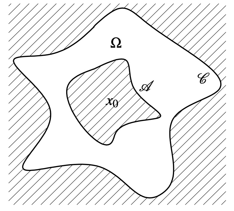
Figure 1: domain $\Omega$

From (2.1) and (2.2), we also see that

$$\bm{n}=-\frac{\nabla H}{|\nabla H|}\quad\text{on ${\mathcal{A}}$},\quad\bm{n}=\frac{\nabla H}{|\nabla H|}\quad\text{on ${\mathcal{C}}$}.$$ (2.3)

It is obvious that the associated stationary problem of (1.1) has the trivial stationary solution

$$(\rho_{i},\rho_{e},\Phi)=(0,0,\lambda H).$$

A simple example is the three-dimensional radial case, the region between two concentric spheres of radius $r_{a}$ for the anode and $r_{c}$ for the cathode. In that case, $H(r)=\frac{r_{c}(r-r_{a})}{r(r_{c}-r_{a})}$ where $r=|x|$.

Notation. For a non-negative integer $k$ and a number $\alpha\in(0,1)$, $C^{k,\alpha}(\overline{\Omega})$ is the Hölder space. We sometimes abbreviate $C^{0,\alpha}(\overline{\Omega})$ by $C^{\alpha}(\overline{\Omega})$. In addition, $C^{k,\alpha}_{0}(\overline{\Omega})$ is a subset of $C^{k,\alpha}(\overline{\Omega})$, whose elements vanish on the boundary $\partial\Omega$. For $1\leq p\leq\infty$, $L^{p}(\Omega)$ is the Lebesgue space. For a non-negative integer $k$, $H^{k}(\Omega)$ is the $k$-th order Sobolev space in $L^{2}$ sense, equipped with the norm $\|\cdot\|_{k}$. Note that $H^{0}(\Omega)=L^{2}(\Omega)$ and we define $\|\cdot\|:=\|\cdot\|_{0}$. The inner product of $L^{2}(\Omega)$ is denoted by $\langle f,g\rangle$ for $f,g\in L^{2}(\Omega)$. Moreover, $H_{0}^{1}(\Omega)$ is closures of $C_{0}^{\infty}(\Omega)$ with respect to $H^{1}$-norm. In the case that $\Omega$ is an annulus or a spherical shell, all the spaces with the subscript $r$, for instance $C^{k,\alpha}_{r}(\overline{\Omega})$, $L^{p}_{r}(\Omega)$, and $H^{k}_{r}(\Omega)$, are subsets whose elements are radial. We denote by $C^{m}([0,T];X)$ the space of the $m$-times continuously differentiable functions on the interval $[0,T]$ with values in a Banach space $X$, and by $H^{m}(0,T;X)$ the space of $H^{m}$–functions on $(0,T)$ with values in a Banach space $X$. Furthermore, we denote by $c$ and $C$ generic positive constants and by $C_{\alpha,\,\beta,\,\cdots}$ a generic positive constant depending on special parameters $\alpha$, $\beta$, $\ldots$.

2.2 Dilute plasma

The stability of the trivial stationary solution $(\rho_{i},\rho_{e},\Phi)=(0,0,\lambda H)$ depends on the following function which involves both the domain $\Omega$ and the rate of pair creation. We define the stability index

$$\kappa(\lambda):=\inf_{u\in H^{1}_{0}(\Omega),u\not\equiv 0}\frac{\displaystyle\int_{\Omega}|\nabla u|^{2}-g(\lambda|\nabla H|)u^{2}dx}{\displaystyle\int_{\Omega}u^{2}dx}$$ (2.4)

for $\lambda>0$, where

$$g(s):=h(s)-\tfrac{s^{2}}{4}=ase^{-\frac{b}{s}}-\tfrac{s^{2}}{4}\ .$$ (2.5)

The sign of $\kappa(\lambda)$ depends on the rate of ion-electron pair creation. For instance, $\kappa(\lambda)<0$ if $a$ is large enough. We also define the self-adjoint linear operator

$$A=-\Delta-g(\lambda|\nabla H|)$$ (2.6)

on $L^{2}(\Omega)$ with domain $H^{2}(\Omega)\cap H^{1}_{0}(\Omega)$. Clearly

$$\kappa(\lambda)\text{ is the lowest eigenvalue of }A.$$

It is well-known that it is a simple eigenvalue and its eigenfunction $\varphi_{1}$ does not vanish in $\Omega$.

It will be convenient to consider $\Phi$ as uniquely determined by $\rho_{i}$ and $\rho_{e}$. We also denote ${\mathcal{R}}=(\rho_{i},\rho_{e})$ and ${\mathcal{R}}_{0}=(\rho_{i0},\rho_{e0})$. We also define the Hilbert space

$$X=H^{2}(\Omega)\times H^{2}(\Omega).$$

Our first theorem asserts that the trivial solution $\rho_{i}=\rho_{e}=V=0$ is asymptotically stable if $\kappa(\lambda)>0$.

Theorem 2.1 (Stability).

Let the stability index $\kappa(\lambda)$ be positive. There exists $\varepsilon>0$ such that if the initial data ${\mathcal{R}}_{0}\in X$ with $\|{\mathcal{R}}_{0}\|_{X}<\varepsilon$ satisfies the compatibility conditions (1.2), then the problem (1.1) has a unique solution ${\mathcal{R}}\in C([0,\infty);X)$ that also satisfies

$$\rho_{i}\in C^{1}([0,\infty);H^{1}(\Omega)),\quad\rho_{i}\geq 0,$$ (2.7a)

$$\rho_{e}\in L^{2}(0,\infty);H^{3}(\Omega))\ \cap\ H^{1}(0,\infty);H^{1}(\Omega)),\quad\rho_{e}\geq 0.$$ (2.7b)

Moreover, there is a constant $C$ such that $\sup_{0\leq t<\infty}\|{\mathcal{R}}(t)\|_{X}\leq C\|{\mathcal{R}}_{0}\|_{X}$ . Furthermore, $\|{\mathcal{R}}(t)\|_{X}$ converges to zero exponentially fast as $t\to\infty$.

Our second theorem asserts that the trivial solution is unstable if $\kappa(\lambda)<0$.

Theorem 2.2 (Instability).

Let the stability index $\kappa(\lambda)$ be negative. There exists $\varepsilon>0$ such that for all $\delta>0$, there exists initial data with $\|{\mathcal{R}}_{0}\|_{X}<\delta$, as well as a time $T>0$ and a solution ${\mathcal{R}}\in C([0,T];X)$ for which $\|{\mathcal{R}}(T)\|_{X}\geq\varepsilon$.

If there are no electrons initially, then there will be no electrons in the future. It has been observed physically that if the initial electron density $\rho_{e0}$ vanishes, then there is no gas discharge. If in addition there are few ions initially, then the ions will also eventually disappear because they will be absorbed by the anode. This is the content of the following proposition.

Proposition 2.3 (No electrons).

Let $\lambda>0$ but make no assumption on $\kappa(\lambda)$. There exists $\varepsilon>0$ such that if the initial data ${\mathcal{R}}_{0}\in X$ satisfy $\rho_{e0}=0$, $\|\rho_{i0}\|_{H^{1}}<\varepsilon$, and the compatibility condition (1.2), then the problem (1.1) has a unique solution ${\mathcal{R}}\in C([0,\infty);X)$ that satisfies (2.7). Furthermore, there exists $T_{0}>0$ such that

$${\mathcal{R}}(t,x)=\bm{0}\quad\text{for}\ \ (t,x)\in[T_{0},\infty)\times\Omega.$$

2.3 Sparking voltage

Definition. The sparking voltage is

$$\lambda^{*}:=\inf\{\lambda>0\ |\ \kappa(\lambda)=0,\ \kappa^{\prime}(\lambda)<0\}.$$ (2.8)

As asserted in the two theorems above, any solution that is initially small converges to the trivial solution as $t$ tends to infinity in case $\lambda<\lambda^{*}$; while it leaves a neighborhood of the trivial solution in case $\lambda>\lambda^{*}$. This means that $\lambda^{*}$ is the threshold of voltage at which gas discharge occurs and continues.

Lemma 2.4.

There exists a sparking voltage $0<\lambda^{*}<\infty$ if $a$ is sufficiently large and $b$ is sufficiently small.

Proof.

The function $g(s)$ defined in (2.5) is either negative for all positive $s$ or it is positive in a finite interval $(s_{1},s_{2})$ in which it has a single local maximum $M$. This can be seen clearly by looking for the function’s zeros. If $s$ is a zero of $g(s)$, then $t=\frac{b}{4a}e^{t}$ where $t=\frac{b}{s}$. The equation for $t$ clearly has at most two zeros. In fact, it has two zeros that are very far apart if the constant $b$ is much smaller than $a$. Furthermore, the maximum $M\to\infty$ as $a\to\infty$. So for large $a$ and small $b$, $g(s)$ has a wide and tall positive hump.

The domain $\Omega$ is fixed. By (2.2) there exist constants $\omega_{1},\omega_{2}$ such that $0<\omega_{1}<|\nabla H(x)|<\omega_{2}$ for all $x\in\Omega$. The operator $-\Delta$ in $\Omega$ with Dirichlet boundary conditions has a smallest eigenvalue $\sigma_{1}>0$ with an eigenfunction $\phi_{1}$. We may normalize $\int_{\Omega}\phi_{1}^{2}\ dx=1$. So $\int|\nabla\phi_{1}|^{2}\ dx=\sigma_{1}$. Fix any number $G>\sigma_{1}$. Due to the wide and tall hump of $g$, we can choose an interval $(\zeta_{1},\zeta_{2})$ between the pair of zeros of $g$ such that

$$g(\zeta_{1})=g(\zeta_{2})=G\quad\text{ and }\quad\frac{\zeta_{2}}{\zeta_{1}}>\frac{\omega_{2}}{\omega_{1}}.$$

Then $g(s)>G$ for all $s\in(\zeta_{1},\zeta_{2})$. Next, we choose $0<\epsilon<\frac{\zeta_{2}}{\omega_{2}}-\frac{\zeta_{1}}{\omega_{1}}$. Let $\lambda_{0}=\frac{\zeta_{1}}{\omega_{1}}+\epsilon$. Then $\zeta_{1}<\lambda_{0}\omega_{1}<\lambda_{0}\omega_{2}<\zeta_{2}$. Because $0<\lambda_{0}\omega_{1}<\lambda_{0}|\nabla H(x)|<\lambda_{0}\omega_{2}$, we have $g(\lambda_{0}|\nabla H(x)|)>G$, for all $x\in\Omega$. Hence

$$\int_{\Omega}\{|\nabla\phi_{1}|^{2}-g(\lambda_{0}|\nabla H|)\ \phi_{1}^{2}\ dx\}<\sigma_{1}-G<0.$$

Choosing $u=\phi_{1}$, it follows that $\kappa(\lambda_{0})<0$. On the other hand, if $\lambda$ is very small, then we see from $\lim_{s\to 0}g(s)=0$ that $\kappa(\lambda)$ is very near $\sigma_{1}$ and is therefore positive. Furthermore, $\kappa$ is a $C^{1}$-function of $\lambda$, so there must be a zero of $\kappa(\cdot)$ between $0$ and $\lambda_{0}$, at which $\kappa^{\prime}(\cdot)<0$ holds. The sparking voltage $\lambda^{*}$ is the smallest positive zero with $\kappa^{\prime}(\lambda^{*})<0$. ∎

2.4 Stationary solutions

Assume now that the sparking voltage $\lambda^{*}>0$ exists. Regarding the voltage $\lambda$ on the cathode ${\mathcal{C}}$ as a bifurcation parameter, we can expect that a one-parameter family of non-trivial stationary solutions may arise from the point $(\lambda,\rho_{i},\rho_{e},\Phi)=(\lambda^{*},0,0,\lambda^{*}H)$. The result on local bifurcation is summarized in Theorem 2.5.

Theorem 2.5 (Local Bifurcation).

Let the positive number $\lambda^{*}$ be defined by (2.8). Then there exists a small number $\eta>0$, as well as $\lambda\in C^{2}([-\eta,\eta];\mathbb{R})$ and $\bm{z}\in C^{2}([-\eta,\eta]\ ;\ C^{1,\alpha}(\overline{\Omega})\times C^{2,\alpha}_{0}(\overline{\Omega})\times C^{3,\alpha}_{0}(\overline{\Omega}))$ such that $\lambda(0)=\lambda^{*}$, $\bm{z}(0)=0$, and such that the associated stationary problem of (1.1) with $\lambda=\lambda(s)$ has a non-trivial solution

$$(\rho_{i},\rho_{e},\Phi)(s)=(s\varphi_{i},s\varphi_{e},s\varphi_{v}+\lambda(s)H)+s\bm{z}(s)$$

for $s\in[-\eta,\eta]$, where $\varphi_{i}\in C^{1,\alpha}(\overline{\Omega})$ is positive, $\varphi_{e}\in C^{2,\alpha}_{0}(\overline{\Omega})$ is positive, and $\varphi_{v}\in C^{3,\alpha}_{0}(\overline{\Omega})$.

On the other hand, in the radial case we can deduce global bifurcation. By the radial case we mean that $\Omega$ is either an annulus $\{(x,y)\in\mathbb{R}^{2};\ r_{1}^{2}<r^{2}:=x^{2}+y^{2}<r_{2}^{2}\}$ or a spherical shell $\{(x,y,z)\in\mathbb{R}^{3};\ r_{1}^{2}<r^{2}:=x^{2}+y^{2}+z^{2}<r_{2}^{2}\}$. The advantage of the radial case is that the system has solutions that depend only on the radial coordinate $r$. When dealing with such solutions, the transport operator, which involves $\nabla\rho_{i}$, depends only on the single derivative $\partial_{r}\rho_{i}$ and not on $\partial_{\theta}\rho_{i}$, so that it is effectively an elliptic operator. Ellipticity is required for compactness in the global bifurcation proof. It is an open problem to prove global bifurcation if $\Omega$ is not radial.

Theorem 2.6 (Global Bifurcation).

Let $\lambda^{*}>0$ satisfy (2.8) and let $\Omega$ be either an annulus ($d=2$) or a spherical shell ($d=3$). Then there exists a unique continuous one-parameter family ${\mathscr{K}}$ (that is, a curve) of radial stationary solutions $(\rho_{i},\rho_{e},\Phi)$ of the problem (1.1). Both densities are positive, $\rho_{i}\in C^{1}_{r},\ \rho_{e}\in C^{2}_{r},\ \Phi\in C^{3}_{r}$, the curve begins at the trivial stationary solution $(\rho_{i},\rho_{e},\Phi)=(0,0,\lambda^{*}H)$ with voltage $\lambda^{*}$ and it “ends” with one of the following two alternatives:

Either (i) the density $\rho_{i}+\rho_{e}$ becomes unbounded along ${\mathscr{K}}$,

Or (ii) the curve ends at a different trivial stationary solution with some voltage $\lambda^{\#}\neq\lambda^{*}$.

Typical bifurcation diagrams are drawn in Figures 2 and 3. More details are given in Theorem 5.11.

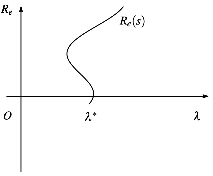
Figure 2: alternative (i)

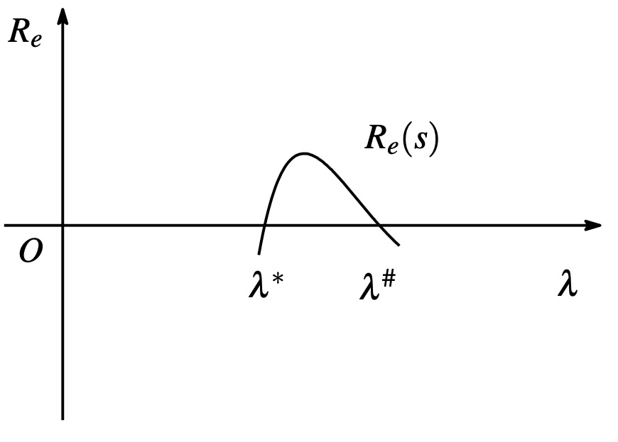
Figure 3: alternative (ii)

This paper is organized as follows. In Section 3 we first make a simple change of variables and some preliminary estimates. The assumption (2.2) on $\Omega$ plays a key role. Then we use the energy method to prove Theorem 2.1 (stability). Next we prove Theorem 2.2 with the stability index being negative, by making use of the lowest eigenfunction of $A$, which leads to a growing mode. For the case of no electrons, we prove by means of the energy method that eventually there are also no ions either (Proposition 2.3).

In Section 4 we easily prove the existence of a local bifurcation curve ${\mathscr{K}}$ of stationary solutions. In Section 5 we prove that ${\mathscr{K}}$ extends to a global curve. It is required to prove Fredholm and compactness conditions. Because the equation for the ion density is not elliptic, the proof of these conditions is restricted to the radial case, that is, a circular cylinder or a spherical shell. Finally we make explicit use of the positivity of the densities in order to show that either ${\mathscr{K}}$ goes from the sparking voltage $\lambda^{*}$ to another voltage $\lambda^{\#}$ or else the densities become unbounded along ${\mathscr{K}}$.

3 Stability analysis of the trivial solution

This section provides the stability analysis of the trivial solution $(\rho_{i},\rho_{e},\Phi)=(0,0,\lambda H)$. It is convenient to rewrite the initial–boundary value problem (1.1) in terms of the modified functions

$$R_{i}:=\rho_{i}e^{-pH},\quad R_{e}:=\rho_{e}e^{\frac{\lambda}{2}H},\quad V:=\Phi-\lambda H,$$ (3.1)

where $p>0$ is a fixed constant to be determined in the proof of Lemma 3.2. We recall that $g(s):=ase^{-\frac{b}{s}}-{s^{2}}/{4}$. As a result, we can rewrite the original problem as

$$\partial_{t}R_{i}+k_{i}\nabla(V+\lambda H)\cdot\nabla R_{i}+pk_{i}\lambda|\nabla H|^{2}R_{i}={k_{e}}h(|\lambda\nabla H|)e^{{-pH}-\frac{\lambda}{2}H}R_{e}+k_{i}f_{i}[R_{i},R_{e},V],$$ (3.2a)

$$\partial_{t}R_{e}-k_{e}\Delta R_{e}-k_{e}g(|\lambda\nabla H|)R_{e}=k_{e}f_{e}[R_{e},V],$$ (3.2b)

$$\Delta V=e^{pH}R_{i}-e^{-\frac{\lambda}{2}H}R_{e}$$ (3.2c)

with the initial and boundary conditions

$$(R_{i},R_{e})(0,x)=(R_{i0},R_{e0})(x),\quad R_{i0}(x)\geq 0,\ R_{e0}(x)\geq 0,$$ (3.2d)

$$R_{i}(t,x)=R_{e}(t,x)=V(t,x)=0,\quad t>0,\ x\in{\mathcal{A}},$$ (3.2e)

$$R_{e}(t,x)=V(t,x)=0,\quad t>0,\ x\in{\mathcal{C}},$$ (3.2f)

where the nonlinear terms $f_{i}$ and $f_{e}$ are defined as

$$f_{i}[R_{i},R_{e},V]:= -(\Delta V+p\nabla V\cdot\nabla H)R_{i}-\frac{k_{e}}{k_{i}}\left\{h(|\lambda\nabla H|)-h(|\nabla V+\lambda\nabla H|)\right\}e^{-pH-\frac{\lambda}{2}H}R_{e},$$

$$f_{e}[R_{e},V]:= \nabla V\cdot\nabla R_{e}-\frac{\lambda}{2}R_{e}\nabla V\cdot\nabla H+R_{e}\Delta V-\left\{h(|\lambda\nabla H|)-h(|\nabla V+\lambda\nabla H|)\right\}R_{e}.$$

The compatibility condition (1.2) can be rewritten as follows:

$$R_{i0}(x)=R_{e0}(x)=(\nabla V(0,x)+\lambda\nabla H(x))\cdot\nabla R_{i0}(x)=0,\quad x\in{\mathcal{A}},$$ (3.3a)

$$R_{e0}(x)=0,\quad x\in{\mathcal{C}},$$ (3.3b)

$$R_{i0}\geq 0,\ R_{e0}\geq 0,\quad x\in\Omega.$$ (3.3c)

The trivial stationary solution is

$$(R_{i},R_{e},V)=(0,0,0).$$

The advantage of using the new unknown functions $R_{i}$ and $R_{e}$ lies in the following two facts. The first one is that the rewritten hyperbolic equation has the dissipative term $pk_{i}\lambda|\nabla H|^{2}R_{i}$ thanks to the assumption (2.2), even though the original hyperbolic equation does not have any dissipative structure. Secondly, the linear part of the rewritten parabolic equation is self-adjoint in $H^{1}_{0}(\Omega)$. These two facts play important roles in the proofs of both the nonlinear stability and instability of the trivial stationary solution. Note that the equations are linear in $(R_{i},R_{e})$ for each $V$.

Now we make a series of straightforward observations. For notational convenience, we define

$$N(T):=\sup_{0\leq t\leq T}\|{\mathcal{R}}(t)\|_{X}=\sup_{0\leq t\leq T}(\|R_{i}(t)\|_{2}+\|R_{e}(t)\|_{2}).$$

By elliptic theory from (3.2c), $V$ is easily estimated as

$$\|V(t)\|_{2+k}{\lesssim_{p}}\|R_{i}(t)\|_{k}+\|R_{e}(t)\|_{k}\quad\text{for}\ \ t\geq 0,\ \ k=0,1,2,$$ (3.4)

$$\|\partial_{t}V(t)\|_{2}{\lesssim_{p}}\|\partial_{t}R_{i}(t)\|+\|\partial_{t}R_{e}(t)\|\quad\text{for}\ \ t\geq 0.$$ (3.5)

The notation $\lesssim_{p}$ means that the constant after $\leq$ may depend on $p$, but not on $T,V,R_{e},R_{i},$ etc. The constant $p$ was introduced in (3.1). Therefore, assuming that $N(T)$ is sufficiently small, and due to (2.1), (2.2), and (3.4) and the boundedness of $\Omega$, there is a constant $c_{1}>0$ depending on $\lambda$ such that

$$(\nabla V+\lambda\nabla H)\cdot\bm{n}\leq-c_{1}\quad \text{on ${\mathcal{A}}$},$$ (3.6)

$$(\nabla V+\lambda\nabla H)\cdot\bm{n}\geq c_{1}\quad \text{on ${\mathcal{C}}$},$$ (3.7)

$$|\nabla H|\geq c_{1}\quad \text{in $\Omega$}.$$ (3.8)

Assuming $N(T)<1$, we can pointwise estimate both nonlinear terms $f_{i}$ and $f_{e}$ in (3.2) as

$$|f_{i}[R_{i},R_{e},V]|\lesssim_{p}(|\nabla V|+|\Delta V|)(|R_{i}|+|R_{e}|)\lesssim_{p}N(T)(|R_{i}|+|R_{e}|),$$ (3.9)

$$|f_{e}[R_{e},V]|\lesssim(|\nabla V|+|\Delta V|)(|R_{e}|+|\nabla R_{e}|){\lesssim_{p}}N(T)(|R_{e}|+|\nabla R_{e}|).$$ (3.10)

The derivatives of $f_{i}$ and $f_{e}$ are also estimated as

$$|\partial_{t}f_{i}[R_{i},R_{e},V]| \lesssim_{p}N(T)(|\partial_{t}R_{i}|+|\partial_{t}R_{e}|+|\partial_{t}\nabla V|+|\partial_{t}\nabla^{2}V|),$$ (3.11)

$$|\nabla f_{i}[R_{i},R_{e},V]| \lesssim_{p}N(T)(|\nabla R_{i}|+|\nabla R_{e}|+|\nabla^{2}V|+|\nabla^{3}V|),$$ (3.12)

$$|\nabla^{2}f_{i}[R_{i},R_{e},V]| \lesssim_{p}|\nabla^{3}V||\nabla R_{i}|+N(T)\sum_{j=1}^{2}(|\nabla^{j}R_{i}|+|\nabla^{j}R_{e}|+|\nabla^{j}V|+|\nabla^{j+1}V|),$$ (3.13)

$$|\partial_{t}f_{e}[R_{e},V]| {\lesssim_{p}}|\partial_{t}\nabla V||\nabla R_{e}|+N(T)(|\partial_{t}R_{e}|+|\partial_{t}\nabla R_{e}|+|\partial_{t}\nabla V|+|\partial_{t}\nabla^{2}V|).$$ (3.14)

Using the estimates (3.9) and (3.10) together with (3.2a), (3.2b), (3.4), and (3.5), we also see for $N(T)<1$ that

$$\|\partial_{t}R_{i}(t)\|+\|\partial_{t}R_{e}(t)\|+\|\partial_{t}V(t)\|_{2}\lesssim_{p}N(T).$$ (3.15)

3.1 Nonlinear stability for $\kappa>0$

Our goal in this subsection is to prove Theorem 2.1. In particular, the smallness assumption on the initial data is required to determine the sign of characteristic of hyperbolic equation (3.2a) as (3.7) and (3.6). This easily leads to the local-in-time solvability of problem (3.2).

Lemma 3.1.

For any $\lambda>0$, there exist an amplitude $\varepsilon>0$ and a time $T>0$ such that if the initial data $(R_{i0},R_{e0})\in H^{2}(\Omega)\times H^{2}(\Omega)$ satisfy $\|R_{i0}\|_{2}+\|R_{e0}\|_{2}<\varepsilon$ and the compatibility condition (3.3), then the problem (3.2) has a unique solution $(R_{i},R_{e},V)$ that satisfies

$$R_{i}\in C([0,T];H^{2}(\Omega))\cap C^{1}([0,\infty);H^{1}(\Omega)),\quad R_{i}\geq 0,$$ (3.16a)

$$R_{e}\in C([0,T];H^{2}(\Omega))\cap L^{2}(0,T;H^{3}(\Omega))\cap H^{1}(0,T;H^{1}(\Omega)),\quad R_{e}\geq 0,$$ (3.16b)

$$V\in C([0,T];H^{4}(\Omega)).$$ (3.16c)

Proof.

We omit the easy proof because it is similar to that of Theorem 2.2 and Remark 2.3 in [22]. ∎

Lemma 3.2.

Let $\kappa(\lambda)>0$. Suppose that $(R_{i},R_{e},V)$ satisfies (3.16) and is a solution to the problem (3.2). There exist $\delta>0$ and $\gamma>0$ such that if $N(T)\leq\delta$, then the following estimate holds for $t\in[0,T]$:

$$e^{{\gamma}t}(\|R_{i}(t)\|_{2}^{2}+\|R_{e}(t)\|_{2}^{2})+\int_{0}^{t}e^{{\gamma}\tau}(\|R_{i}(\tau)\|_{2}^{2}+\|R_{e}(\tau)\|_{2}^{2})\,d\tau\lesssim\|R_{i0}\|_{2}^{2}+\|R_{e0}\|_{2}^{2}.$$ (3.17)

Recall that $\|\cdot\|_{k}$ denotes the norm of $H^{k}(\Omega)$. We emphasize that the constant in $\lesssim$ is independent of $T$.

Proof of Theorem 2.1, assuming Lemma 3.2.

The global-in-time solution $(R_{i},R_{e},\!V)$ with (3.16) is constructed by a standard continuation argument using the time local solvability established in Lemma 3.1 and the a priori estimate in Lemma 3.2. Once the global solution is constructed, it is obvious that the resulting global solution satisfies the estimate (3.17) for all $t\in[0,\infty)$. We conclude that the global solution decays exponentially fast in $X$ as $t$ goes to infinity. Of course, it follows from (3.4) that $\|V(t)\|_{4}$ also decays exponentially. These facts together with (3.1) immediately ensure Theorem 2.1. ∎

Now we begin the rather long proof of Lemma 3.2.

Proof of Lemma 3.2..

First we estimate $R_{e}$ in $L^{2}$. We multiply (3.2b) by $2e^{\gamma t}R_{e}$ for some $\gamma\in(0,1)$, integrate it by parts over $[0,t]\times\Omega$, and use the boundary conditions (3.2e) and (3.2f) as well as the estimate (3.10) to obtain

$$e^{\gamma t}\int_{\Omega}{R}_{e}^{2}\,dx+2k_{e}\int_{0}^{t}\!\!\int_{\Omega}e^{\gamma\tau}\left(|\nabla R_{e}|^{2}-g(|\lambda\nabla H|){R}_{e}^{2}\right)\,dxd\tau$$

$$=\int_{\Omega}{R}_{e0}^{2}\,dx+\gamma\int_{0}^{t}\!\!\int_{\Omega}e^{\gamma\tau}R_{e}^{2}\,dxd\tau+2k_{e}\int_{0}^{t}\!\!\int_{\Omega}e^{\gamma\tau}f_{e}R_{e}\,dxd\tau$$

$$\leq\|R_{e0}\|^{2}+(\gamma+{C_{p}N(T)})\int_{0}^{t}e^{\gamma\tau}\|R_{e}(\tau)\|^{2}_{1}\,d\tau,$$ (3.18)

where the constant $C_{p}>0$ depends on $p$. Because $\kappa(\lambda)>0$, there exists a constant $c_{2}>0$ such that

$$\int_{\Omega}|\nabla u|^{2}-g(|\lambda\nabla H|)u^{2}dx\geq c_{2}\|u\|_{1}^{2}\quad\text{for}\ \ u\in H^{1}_{0}(\Omega).$$ (3.19)

Applying this inequality (3.19) to the second term on the left side of (3.18) and then taking $\gamma>0$ and $N(T)$ sufficiently small, we arrive at

$$e^{\gamma t}\|R_{e}(t)\|^{2}+\int_{0}^{t}e^{\gamma\tau}\|R_{e}(\tau)\|_{1}^{2}\,d\tau\lesssim\|R_{0e}\|^{2}.$$ (3.20)

Here we have taken $\gamma$ independent of $p$. Next we multiply (3.2b) by $2e^{\gamma t}\partial_{t}R_{e}$, integrate it by parts over $[0,t]\times\Omega$, use the boundary conditions (3.2e) and (3.2f) as well as the estimate (3.10) and the Schwarz inequality, and take $N(T)$ small to obtain

$$e^{\gamma t}k_{e}\int_{\Omega}|\nabla{R}_{e}|^{2}\,dx+2\int_{0}^{t}\!\!\int_{\Omega}e^{\gamma\tau}|\partial_{t}R_{e}|^{2}\,dxd\tau$$

$$=k_{e}\int_{\Omega}|\nabla{R}_{e0}|^{2}\,dx+\gamma k_{e}\int_{0}^{t}\!\!\int_{\Omega}e^{\gamma\tau}|\nabla R_{e}|^{2}\,dxd\tau+2k_{e}\int_{0}^{t}\!\!\int_{\Omega}e^{\gamma\tau}(g(|\lambda\nabla H|)R_{e}+f_{e})\partial_{t}R_{e}\,dxd\tau$$

$$\leq\int_{0}^{t}\!\!\int_{\Omega}e^{\gamma\tau}|\partial_{t}R_{e}|^{2}\,dxd\tau+C\|\nabla R_{e0}\|^{2}+C\int_{0}^{t}e^{\gamma\tau}\|R_{e}(\tau)\|^{2}_{1}\,d\tau.$$ (3.21)

From this estimate and (3.20), it follows that

$$e^{\gamma t}\|\nabla R_{e}(t)\|^{2}+\int_{0}^{t}e^{\gamma\tau}\|\partial_{t}R_{e}(\tau)\|^{2}\,d\tau\lesssim\|R_{0e}\|_{1}^{2}.$$ (3.22)

Furthermore, we apply $\partial_{t}$ to (3.2b), multiply the resulting equation by $2e^{\gamma t}\partial_{t}R_{e}$, and integrate it by parts over $[0,t]\times\Omega$ to obtain

$$e^{\gamma t}\int_{\Omega}|\partial_{t}{R}_{e}|^{2}\,dx+2k_{e}\int_{0}^{t}\!\!\int_{\Omega}e^{\gamma\tau}\left(|\partial_{t}\nabla R_{e}|^{2}-g(|\lambda\nabla H|)|\partial_{t}{R}_{e}|^{2}\right)\,dxd\tau$$

$$=\int_{\Omega}|\partial_{t}{R}_{e}|^{2}(0,x)\,dx+\gamma\int_{0}^{t}\!\!\int_{\Omega}e^{\gamma\tau}|\partial_{t}R_{e}|^{2}\,dxd\tau+2k_{e}\int_{0}^{t}\!\!\int_{\Omega}e^{\gamma\tau}(\partial_{t}f_{e})(\partial_{t}R_{e})\,dxd\tau$$

$$\leq\|R_{e0}\|_{2}^{2}+(\gamma+{C_{p}N(T)})\int_{0}^{t}e^{\gamma\tau}(\|\partial_{t}R_{e}(\tau)\|_{1}^{2}+\|\partial_{t}R_{i}(\tau)\|^{2})\,d\tau,$$ (3.23)

where we have also used (3.2b), (3.5), and (3.14) as well as the Schwarz and Sobolev inequalities. Then using (3.19) and taking $\gamma$ and $N(T)$ small, we arrive at

$$e^{\gamma t}\|\partial_{t}R_{e}(t)\|^{2}+\int_{0}^{t}e^{\gamma\tau}\|\partial_{t}R_{e}(\tau)\|_{1}^{2}\,d\tau\lesssim\|R_{0e}\|_{2}^{2}+\int_{0}^{t}e^{\gamma\tau}\|\partial_{t}R_{i}(\tau)\|^{2}\,d\tau.$$ (3.24)

Hereafter we fix $\gamma>0$ so that (3.20), (3.22), and (3.24) hold. We note that $\gamma$ is independent of $p$.

Now let us estimate $R_{i}$. Choose $p>0$ so large that $2p\lambda k_{i}c_{1}>\gamma$, where $c_{1}$ is the constant in (3.8). We multiply (3.2a) by $2e^{\gamma t}R_{i}$, integrate by parts over $[0,t]\times\Omega$, and use the boundary condition (3.2e) to obtain

$$e^{\gamma t}\int_{\Omega}R_{i}^{2}\,dx+\int_{0}^{t}\!\!\int_{\Omega}e^{\gamma\tau}(2p\lambda k_{i}|\nabla H|^{2}-\gamma)R_{i}^{2}\,dxd\tau+k_{i}\int_{0}^{t}\!\!\int_{{\mathcal{C}}}e^{\gamma\tau}R_{i}^{2}\nabla(V+\lambda H)\cdot\bm{n}\,dSd\tau$$

$$=\int_{\Omega}R_{i0}^{2}\,dx+k_{i}\int_{0}^{t}\!\!\int_{\Omega}e^{\gamma\tau}R_{i}^{2}\Delta V\,dxd\tau+2\int_{0}^{t}\!\!\int_{\Omega}e^{\gamma\tau}\left({k_{e}}h(|\lambda\nabla H|)e^{-pH-\frac{\lambda}{2}H}R_{e}+k_{i}f_{i}\right)R_{i}\,dxd\tau$$

$$\lesssim_{p}\|R_{i0}\|^{2}+(\mu+N(T))\int_{0}^{t}e^{\gamma\tau}\|R_{i}(\tau)\|^{2}\,d\tau+\mu^{-1}\int_{0}^{t}e^{\gamma\tau}\|R_{e}(\tau)\|^{2}\,d\tau,$$ (3.25)

where $\mu$ is a positive constant, and we have used (3.4) and (3.9) as well as the Schwarz and Sobolev inequalities. From (3.8) and $2p\lambda k_{i}c_{1}>\gamma$, it is seen that the coefficient $(2p\lambda k_{i}|\nabla H|^{2}-\gamma)$ in the second term on the left hand side of (3.25) is positive. Owing to (3.7), the third term on the left side of (3.25) (the integral over ${\mathcal{C}}$) is non-negative and thus can be dropped. Then letting $\mu$ and $N(T)$ be sufficiently small and using (3.20), we arrive at

$$e^{\gamma t}\|R_{i}(t)\|^{2}+\int_{0}^{t}e^{\gamma\tau}\|R_{i}(\tau)\|^{2}\,d\tau\lesssim_{p}\|R_{i0}\|^{2}+\|R_{e0}\|^{2}.$$ (3.26)

Next we apply the temporal derivative $\partial_{t}$ to (3.2a), multiply the resulting equation by $2e^{\gamma t}\partial_{t}R_{i}$, and integrate by parts over $[0,t]\times\Omega$ to obtain

$$e^{\gamma t}\int_{\Omega}|\partial_{t}R_{i}|^{2}\,dx+\int_{0}^{t}\!\!\int_{\Omega}e^{\gamma\tau}(2p\lambda k_{i}|\nabla H|^{2}-\gamma)|\partial_{t}R_{i}|^{2}\,dxd\tau+k_{i}\int_{0}^{t}\!\!\int_{{\mathcal{C}}}e^{\gamma\tau}|\partial_{t}R_{i}|^{2}\nabla(V+\lambda H)\cdot\bm{n}\,dSd\tau$$

$$=\int_{\Omega}|\partial_{t}R_{i}|^{2}|(0,x)\,dx+k_{i}\int_{0}^{t}\!\!\int_{\Omega}e^{\gamma\tau}|\partial_{t}R_{i}|^{2}\Delta V\,dxd\tau-k_{i}\int_{0}^{t}\!\!\int_{\Omega}e^{\gamma\tau}(\partial_{t}\nabla V\cdot\nabla R_{i})\partial_{t}R_{i}\,dxd\tau$$

$$\quad+2\int_{0}^{t}\!\!\int_{\Omega}e^{\gamma\tau}\left({k_{e}}h(|\lambda\nabla H|)e^{-pH-\frac{\lambda}{2}H}\partial_{t}R_{e}+k_{i}\partial_{t}f_{i}\right)\partial_{t}R_{i}\,dxd\tau$$

$$\lesssim_{p}\|R_{i0}\|_{1}^{2}+\|R_{e0}\|^{2}+(\mu+N(T))\int_{0}^{t}e^{\gamma\tau}\|\partial_{t}R_{i}(\tau)\|^{2}\,d\tau+\mu^{-1}\int_{0}^{t}e^{\gamma\tau}\|\partial_{t}R_{e}(\tau)\|^{2}\,d\tau,$$ (3.27)

where we have used (3.4), (3.5), and (3.11) as well as the Schwarz and Sobolev inequalities. From (3.8) and $2p\lambda k_{i}c_{1}>\gamma$, it is seen that the coefficient $(2p\lambda k_{i}|\nabla H|^{2}-\gamma)$ in the second term on the left hand side of (3.25) is positive. Owing to (3.7), the third term on the left hand side of (3.25) is non-negative and thus can be dropped. Then letting $\mu$ and $N(T)$ be sufficiently small and using (3.22), we see that

$$e^{\gamma t}\|\partial_{t}R_{i}(t)\|^{2}+\int_{0}^{t}e^{\gamma\tau}\|\partial_{t}R_{i}(\tau)\|^{2}\,d\tau\lesssim_{p}\|R_{i0}\|_{1}^{2}+\|R_{e0}\|_{1}^{2}.$$ (3.28)

It remains to take the spatial derivatives. That is, we will prove the estimate

$$e^{\gamma t}\|\nabla^{k}R_{i}(t)\|^{2}+\int_{0}^{t}e^{\gamma\tau}\|\nabla^{k}R_{i}(\tau)\|^{2}\,d\tau\lesssim_{p}\|R_{i0}\|_{2}^{2}+\|R_{e0}\|_{2}^{2}+\int_{0}^{t}e^{\gamma\tau}\|R_{e}(\tau)\|^{2}_{2}\,d\tau$$ (3.29)

for $k=1,2$. Lemma 3.2 follows from (3.29). Indeed, in order to complete the proof of Lemma 3.2, we regard the parabolic equation (3.2b) as the Poisson equation to obtain the elliptic estimate

$$\|R_{e}\|_{2}\lesssim\|\partial_{t}R_{e}\|+\|R_{e}\|_{1}.$$ (3.30)

Combining (3.20), (3.22), (3.24), (3.26), and (3.28), and then applying (3.30), we have

$$e^{\gamma t}\left(\|R_{i}(t)\|^{2}+\|R_{e}(t)\|_{2}^{2}\right)+\int_{0}^{t}e^{\gamma\tau}\left(\|R_{i}(\tau)\|^{2}+\|R_{e}(\tau)\|_{2}^{2}\right)\,d\tau\lesssim_{p}\|R_{i0}\|_{2}^{2}+\|R_{e0}\|_{2}^{2}.$$

This estimate and (3.29) immediately yield (3.17). ∎

Proof of (3.29).

In order to take spatial derivatives we must be careful about the boundary. So we use local coordinates near the anode ${\mathcal{A}}$. We will cover ${\mathcal{A}}$ by a fixed number of small balls $V_{j},j=1,...,N$ and cover the rest of $\Omega$ by one open set $V_{0}$. The we will choose a partial of unity $\{\zeta_{j}\}$ for $V_{0},V_{1},...,V_{N}$. Furthermore we will choose maps $\bm{\Phi_{j}}$ that locally flatten the boundary.

Now we make this procedure explicit. For any $\varepsilon_{0}>0$, dimension $d=2,3$, and $0\leq j\leq N$, we choose the domain $V_{j}$, the functions $\zeta_{j}$, ${\zeta}_{j}^{\prime}$, the bijection map $\bm{\Phi}_{j}:\mathbb{R}^{d}\to\mathbb{R}^{d}$ and its inverse map $\bm{\Psi}_{j}:\mathbb{R}^{d}\to\mathbb{R}^{d}$, to satisfy the following properties.

1. For $0\leq j\leq N$, both $\bm{\Psi}_{j}$ and $\bm{\Phi}_{j}$ belong to $C^{3}(\mathbb{R}^{d})$ and $|\mathop{\rm det}\nolimits\nabla\bm{\Phi}_{j}|=1$, $|\mathop{\rm det}\nolimits\nabla\bm{\Psi}_{j}|=1$. Moreover, $\nabla\bm{\Phi}_{j}=T_{j}+S_{j}$, and $\nabla\bm{\Psi}_{j}={}^{t}T_{j}+S_{j}^{\star}$, where $T_{j}$ is a constant orthonormal matrix and $S_{j},S_{j}^{\star}\in C^{2}(\mathbb{R}^{d})$ are $n\times n$ matrix functions with $\|S_{j}\|_{L^{\infty}}+\|S_{j}^{\star}\|_{L^{\infty}}\leq\varepsilon_{0}$. Furthermore, $\nabla^{2}\bm{\Phi}_{j},\nabla^{2}\bm{\Psi}_{j}\in W^{1,\infty}({\mathbb{R}}^{d})$.

2. $V_{0}\subset\Omega$, while for $j\neq 0$, we assume $\Omega\cap V_{j}=\bm{\Phi}_{j}(\mathbb{R}^{d}_{+})\cap V_{j}$, and ${\mathcal{A}}\cap V_{j}=\bm{\Phi}_{j}(\partial\mathbb{R}^{d}_{+})\cap V_{j}$.

3. ${\rm supp}\zeta_{j}\subset{\rm supp}\zeta^{\prime}_{j}\subset V_{j}$ and $\zeta^{\prime}_{j}=1$ on ${\rm supp}\zeta_{j}$. There exist constants $\sigma>0$ and $L>0$ such that $\sum_{j=0}^{N}\zeta_{j}(x)=1$ for $x\in\Omega_{\sigma}$, $\sum_{j=1}^{N}\zeta_{j}(x)=1$ for $x\in{\mathcal{A}}_{\sigma}$, and ${\rm supp}\nabla\zeta_{j}\subset\{x\,|\,|x|\leq L\}$ for $j=0,\ldots,N$, where $\Omega_{\sigma}=\{x\in\mathbb{R}^{d};{\rm dist}(x,\Omega)\leq\sigma\}$ and ${\mathcal{A}}_{\sigma}=\{x\in\mathbb{R}^{d};{\rm dist}(x,{\mathcal{A}})\leq\sigma\}$.

4. For $j\neq 0$, $\tilde{\bm{n}}(x)\cdot\nabla_{x}f=-(\partial_{y_{d}}f+\bm{r}_{j}(y)\cdot\nabla_{y}f)$ for $x\in\Omega\cap V_{j}$ and $y=\bm{\Psi}_{j}(x)$, where $\tilde{\bm{n}}:=-\nabla H/|\nabla H|$, the restriction of $\tilde{\bm{n}}$ on ${\mathcal{A}}$ is a normal unit vector of ${\mathcal{A}}$ (see (2.3)), and the vector $\bm{r}_{j}=(r_{j1},\cdots,r_{jd})\in C^{2}(\bm{\Psi}_{j}(\Omega\cap V_{j}))\cap W^{2,\infty}(\bm{\Psi}_{j}(\Omega\cap V_{j}))$ satisfies $\|\bm{r}_{j}\|_{L^{\infty}}\leq\varepsilon_{0}$.

Hereafter we set $\varepsilon_{0}=\frac{1}{2}$.

First let us consider the estimate of $R_{i}$ away from the anode ${\mathcal{A}}$ by using the cut-off function $\zeta_{0}$. We apply a first or second derivative $\partial^{\alpha}=\partial^{\alpha}_{x}$ to the problem (3.2a) to obtain an equation for $\partial^{\alpha}R_{i}$, namely:

$$\partial_{t}(\partial^{\alpha}{R}_{i})+k_{i}\nabla(V+\lambda H)\cdot\nabla(\partial^{\alpha}{R}_{i})+pk_{i}\lambda|{\nabla}{H}|^{2}(\partial^{\alpha}{R}_{i})$$

$$=\partial^{\alpha}\left\{{k_{e}}h(|\lambda{\nabla}{H}|)e^{-p{H}-\frac{\lambda}{2}{H}}{R}_{e}\right\}+k_{i}\partial^{\alpha}{f}_{i}+{\cal R}_{\alpha},$$

where the commutators ${\cal R}_{\alpha}$ are defined by

$${\cal R}_{\alpha} :=k_{i}[\partial^{\alpha},\nabla(V+\lambda H)\cdot{\nabla}]{R}_{i}+pk_{i}\lambda[\partial^{\alpha},|{\nabla}{H}|^{2}]{R}_{i}.$$

We multiply this equation by $2e^{\gamma t}\zeta_{0}^{2}\partial^{\alpha}{R}_{i}$ and integrate by parts over $[0,t]\times\Omega$ to obtain he following estimate (which is analogous to (3.25)):

$$e^{\gamma t}\int_{\Omega}\zeta_{0}^{2}|\partial^{\alpha}R_{i}|^{2}\,dx+\int_{0}^{t}\!\!\int_{\Omega}e^{\gamma\tau}\zeta_{0}^{2}(2p\lambda k_{i}|\nabla H|^{2}-\gamma)|\partial^{\alpha}R_{i}|^{2}\,dxd\tau$$

$$\quad+k_{i}\int_{0}^{t}\!\!\int_{{\mathcal{C}}}e^{\gamma\tau}\zeta_{0}^{2}|\partial^{\alpha}R_{i}|^{2}\nabla(V+\lambda H)\cdot\bm{n}\,dSd\tau$$

$$=\int_{\Omega}\zeta_{0}^{2}|\partial^{\alpha}R_{i0}|^{2}\,dx+k_{i}\int_{0}^{t}\!\!\int_{\Omega}e^{\gamma\tau}\zeta_{0}^{2}|\partial^{\alpha}R_{i}|^{2}\nabla\cdot\left\{\zeta_{0}^{2}\nabla(V+\lambda H)\right\}\,dxd\tau$$

$$\quad+2\int_{0}^{t}\!\!\int_{\Omega}e^{\gamma\tau}\zeta_{0}^{2}\left[\partial^{\alpha}\left\{{k_{e}}h(|\lambda{\nabla}{H}|)e^{-p{H}-\frac{\lambda}{2}{H}}{R}_{e}\right\}+k_{i}\partial^{\alpha}f_{i}+{\cal R}_{\alpha}\right]\partial^{\alpha}R_{i}\,dxd\tau$$

$$\leq\tilde{C}\|R_{i0}\|_{2}^{2}+\tilde{C}\int_{0}^{t}e^{\gamma\tau}\|\nabla^{|\alpha|}R_{i}(\tau)\|^{2}\,d\tau+C_{p}\int_{0}^{t}e^{\gamma\tau}\|R_{i}(\tau)\|_{|\alpha|-1}^{2}\,d\tau$$

$$\quad+C_{p}N(T)\int_{0}^{t}e^{\gamma\tau}\|R_{i}(\tau)\|^{2}_{|\alpha|}\,d\tau+C_{p}\int_{0}^{t}e^{\gamma\tau}\|R_{e}(\tau)\|_{2}^{2}\,d\tau,$$ (3.31)

where we have used (3.4), (3.12), and (3.13) as well as the Schwarz and Sobolev inequalities. Here $\tilde{C}>0$ is a constant independent of $p$. We note that the coefficient $(2p\lambda k_{i}|\nabla H|^{2}-\gamma)$ in the second term on the left hand side of (3.31) is positive. Furthermore, owing to (3.7), the third term on the left hand side of (3.31) is non-negative and thus can be dropped.

Next we deal with the estimate of $R_{i}$ near the anode ${\mathcal{A}}$. In the region $V_{j}$ for a fixed $j$ we use the local coordinate $y=\bm{\Psi}_{j}(x)$. We choose $\varepsilon_{0}=\frac{1}{2}$. We define

$$(\hat{R}_{i},\hat{R}_{e},\hat{V})(t,y):=(R_{e},R_{i},V)(t,\bm{\Phi}_{j}(y)),\quad(\hat{H},\hat{\zeta}_{j},\hat{\zeta}_{j}^{\prime})(y):=(H,\zeta,\zeta^{\prime})(\bm{\Phi}_{j}(y)),$$

$$\hat{\nabla}:=\nabla\bm{\Psi}_{j}\nabla_{y}.$$

Then from (3.2) and property (iv) of the local coordinate we have the transformed equation

$$\begin{aligned} &\partial_{t}\hat{R}_{i}+k_{i}\lambda|\hat{\nabla}\hat{H}|(\partial_{y_{d}}\hat{R}_{i}+\bm{r}_{j}\cdot\nabla_{y}\hat{R}_{i})+k_{i}\hat{\nabla}\hat{V}\cdot\hat{\nabla}\hat{R}_{i}+pk_{i}\lambda|\hat{\nabla}\hat{H}|^{2}\hat{R}_{i}\\ &={k_{e}}h(|\lambda\hat{\nabla}\hat{H}|)e^{-p\hat{H}-\frac{\lambda}{2}\hat{H}}\hat{R}_{e}+k_{i}\hat{f}_{i},\end{aligned}$$ (3.32a)

$$\hat{R}_{i}(0,y)=\hat{R}_{i0}(y):=R_{i0}(\bm{\Phi}_{j}(y)),$$ (3.32b)

$$\hat{R}_{i}(t,y_{1},y_{2},0)=0,$$ (3.32c)

where $t>0$ and $y\in\bm{\Psi}_{j}(\Omega\cap V_{j})$. We note that for $c_{1}$ defined in (3.8),

$$|\hat{\nabla}\hat{H}(y)|=|\nabla_{x}H(\bm{\Phi}_{j}(y))|\geq c_{1}>0,\quad y\in\bm{\Psi}_{j}(\Omega\cap V_{j}).$$

For notational convenience, we may express $\hat{\nabla}\hat{V}\cdot\hat{\nabla}$ as

$$\hat{\nabla}\hat{V}\cdot\hat{\nabla}=\sum_{l=1}^{d}a_{l}(\nabla_{y}\bm{\Psi}_{j},\hat{\nabla}\hat{V})\partial_{y_{l}},\quad\text{where}\quad|a_{l}(\nabla_{y}\bm{\Psi}_{j},\hat{\nabla}\hat{V})|\lesssim|\hat{\nabla}\hat{V}|.$$

We finally apply the spatial derivatives $\partial^{\alpha}=\partial^{\alpha}_{y}$ (say for dimension 3) to the problem (3.32) to obtain

$$\begin{aligned} &\partial_{t}(\partial^{\alpha}\hat{R}_{i})+k_{i}\lambda|\hat{\nabla}\hat{H}|\{\partial_{y_{3}}(\partial^{\alpha}\hat{R}_{i})+\bm{r}_{j}\cdot\nabla_{y}(\partial^{\alpha}\hat{R}_{i})\}+k_{i}\hat{\nabla}\hat{V}\cdot\hat{\nabla}(\partial^{\alpha}\hat{R}_{i})+pk_{i}\lambda|\hat{\nabla}\hat{H}|^{2}(\partial^{\alpha}\hat{R}_{i})\\ &=\partial^{\alpha}\left\{{k_{e}}h(|\lambda\hat{\nabla}\hat{H}|)e^{-p\hat{H}-\frac{\lambda}{2}\hat{H}}\hat{R}_{e}\right\}+k_{i}\partial^{\alpha}\hat{f}_{i}+{\cal R}_{\alpha}^{\prime},\end{aligned}$$ (3.33a)

$$\partial^{\alpha}\hat{R}_{i}(0,y)=\partial^{\alpha}\hat{R}_{i0}(y),$$ (3.33b)

$$\partial^{\alpha}\hat{R}_{i}(t,y_{1},y_{2},0)=\left\{\begin{array}[]{ll}{\cal B}={\cal B}(t,y_{1},y_{2},0)&\text{if $\alpha=(0,0,2)$},\\ 0&\text{otherwise},\end{array}\right.$$ (3.33e)

where the commutators ${\cal R}_{\alpha}^{\prime}$ and the boundary data ${\cal B}$ are defined by

$${\cal R}_{\alpha}^{\prime} :=k_{i}\lambda\left[\partial^{\alpha},|\hat{\nabla}\hat{H}|\partial_{y_{3}}\right]\hat{R}_{i}+k_{i}\lambda\left[\partial^{\alpha},|\hat{\nabla}\hat{H}|\bm{r}_{j}\cdot\nabla_{y}\right]\hat{R}_{i}+k_{i}\left[\partial^{\alpha},\hat{\nabla}\hat{V}\cdot\hat{\nabla}\right]\hat{R}_{i}$$

$$\quad+pk_{i}\lambda\left[\partial^{\alpha},|\hat{\nabla}\hat{H}|^{2}\right]\hat{R}_{i},$$

$${\cal B} :=\frac{k_{e}\partial_{y_{3}}\left\{h(|\hat{\nabla}\hat{V}+\lambda\hat{\nabla}\hat{H}|)e^{-p\hat{H}-\frac{\lambda}{2}\hat{H}}\hat{R}_{e}\right\}}{k_{i}\left\{\lambda|\hat{\nabla}\hat{H}|(1+r_{j3})+a_{3}\right\}}(t,y_{1},y_{2},0).$$

Here we have used (3.32a), (3.32c), $\hat{R}_{e}(t,y_{1},y_{2},0)=0$, $\|\bm{r}_{j}\|_{L^{\infty}}\leq\frac{1}{2}$, and $|a_{3}|\lesssim|\hat{\nabla}\hat{V}|\lesssim N(T)\ll 1$ in deriving $\partial_{y_{3}}\hat{R}_{i}(t,y_{1},y_{2},0)=0$. We have used (3.33a) with $\alpha=(0,0,1)$ and (3.33e) with $|\alpha|=1$ in deriving $\partial_{y_{3}}^{2}\hat{R}_{i}(t,y_{1},y_{2},0)=\cal B$. The standard trace theorem gives

$$\|\hat{\zeta}_{j}^{\prime}{\cal B}(t,y_{1},y_{2},0)\|_{L^{2}(\mathbb{R}^{2}_{+})}\lesssim\|R_{e}\|_{2},$$ (3.34)

where we have also used $\|\bm{r}_{j}\|_{L^{\infty}}\leq\frac{1}{2}$ and $|a_{3}|\lesssim|\hat{\nabla}\hat{V}|\lesssim N(T)\ll 1$ to ensure the positivity of the denominator of $\cal B$.

Now we multiply (3.33a) by $2e^{\gamma t}\hat{\zeta}_{j}^{2}\partial^{\alpha}\hat{R}_{i}$ and integrate by parts over $[0,t]\times\mathbb{R}^{3}_{+}$ to obtain

$$e^{\gamma t}\int_{\mathbb{R}^{3}_{+}}\hat{\zeta}_{j}^{2}|\partial^{\alpha}\hat{R}_{i}|^{2}\,dy+\int_{0}^{t}\!\!\int_{\mathbb{R}^{3}_{+}}e^{\gamma\tau}\hat{\zeta}_{j}^{2}(2p\lambda k_{i}|\hat{\nabla}\hat{H}|^{2}-\gamma)|\partial^{\alpha}\hat{R}_{i}|^{2}\,dyd\tau$$

$$=\int_{\Omega}\hat{\zeta}_{j}^{2}|\partial_{\alpha}\hat{R}_{i0}|^{2}\,dy+k_{i}\int_{0}^{t}\!\!\int_{\mathbb{R}^{2}}e^{\gamma\tau}\hat{\zeta}_{j}^{2}\left\{\lambda|\hat{\nabla}\hat{H}|(1+r_{j3})+a_{3}\right\}|\partial^{\alpha}\hat{R}_{i}|^{2}(t,y_{1},y_{2},0)dy_{1}dy_{2}d\tau$$

$$\quad+k_{i}\int_{0}^{t}\!\!\int_{\mathbb{R}^{3}_{+}}e^{\gamma\tau}|\partial^{\alpha}\hat{R}_{i}|^{2}\sum_{l=1}^{3}\partial_{y_{l}}\left[\hat{\zeta}_{j}^{2}\left\{\lambda|\hat{\nabla}\hat{H}|(\delta_{3l}+r_{jl})+a_{l}\right\}\right]\,dyd\tau$$

$$\quad+2\int_{0}^{t}\!\!\int_{\mathbb{R}^{3}_{+}}e^{\gamma\tau}\hat{\zeta}_{j}^{2}\left(\partial^{\alpha}\left\{{k_{e}}h(|\lambda\hat{\nabla}\hat{H}|)e^{-p\hat{H}-\frac{\lambda}{2}\hat{H}}\hat{R}_{e}\right\}+k_{i}\partial^{\alpha}\hat{f}_{i}+{\cal R}_{\alpha}^{\prime}\right)\partial^{\alpha}\hat{R}_{i}\,dyd\tau$$

$$\leq\tilde{C}\|R_{i0}\|_{2}^{2}+\tilde{C}\int_{0}^{t}e^{\gamma\tau}\|\nabla^{|\alpha|}R_{i}(\tau)\|^{2}\,d\tau+C_{p}\int_{0}^{t}e^{\gamma\tau}\|R_{i}(\tau)\|_{|\alpha|-1}^{2}\,d\tau$$

$$\quad+C_{p}N(T)\int_{0}^{t}e^{\gamma\tau}\|R_{i}(\tau)\|^{2}_{|\alpha|}\,d\tau+C_{p}\int_{0}^{t}e^{\gamma\tau}\|R_{e}(\tau)\|_{2}^{2}\,d\tau,$$ (3.35)

where we have used (3.4), (3.12), (3.13), (3.33e), (3.34), and ${\rm supp}\zeta^{\prime}_{j}=1$ on ${\rm supp}\zeta_{j}$ as well as the Schwarz and Sobolev inequalities. Here $\tilde{C}>0$ is a constant independent of $p$. We note that the coefficient $(2p\lambda k_{i}|\nabla\hat{H}|^{2}-\gamma)$ in the second term on the left hand side of (3.31) is positive.

We are finally able to prove (3.29). We recall that the second terms on the left sides of (3.31) and (3.35) provide good contributions, while the third term on the left side of (3.31), which is an integral over ${\mathcal{C}}$, can be dropped. We sum up $\eqref{apes14}$ and $\eqref{apes13}$ for $j=1,\ldots,N$ and $\alpha$ with $|\alpha|=1$. Then we take $p$ sufficiently large to absorb the term $\tilde{C}\int_{0}^{t}e^{\gamma\tau}\|\nabla^{|\alpha|}R_{i}(\tau)\|^{2}\,d\tau$ into the good contribution on the left hand side of the resulting inequality, and also let $N(T)$ be small relative to $p$. Using (3.26), we finally arrive at (3.29) with $k=1$. In a similar fashion we obtain (3.29) for $k=2$. ∎

3.2 Nonlinear instability for $\kappa<0$

This subsection provides the proof of Theorem 2.2. The key assumption is that $\kappa(\lambda)<0$. Recall that the self-adjoint operator $A=-\Delta-g(\lambda\nabla H)$ has its lowest eigenvalue $-\mu_{1}=\kappa(\lambda)$ with an eigenfunction denoted by $\varphi_{1}$. Then $\varphi_{1}$ does not vanish so we may assume it is positive in $\Omega$ and $\|\varphi_{1}\|=1$.

For convenience, we choose initial data ${\mathcal{R}}_{0}=(\delta\psi_{i},\delta\psi_{e})\in X$ that satisfies the compatibility condition (3.3), as well as

$$\psi_{i},\psi_{e}\geq 0,\quad\psi_{e}\not\equiv 0,\quad\|\psi_{i}\|_{1}^{2}+\|\psi_{e}\|_{1}^{2}=1.$$ (3.36)

Lemma 3.3.

Let $\kappa(\lambda)<0$. There exists $\varepsilon_{0}>0$ such that if the solution $(R_{i},R_{e})$ of problem (3.2) with $(R_{i0},R_{e0})=(\delta\psi_{i},\delta\psi_{e})$ for some $\delta\in(0,\varepsilon_{0})$ satisfies $N(T)\leq\varepsilon_{0}$ and if

$$\left\|R_{e}(t)-\delta e^{k_{e}tA}\psi_{e}\right\|\leq\delta e^{-\kappa(\lambda)k_{e}t}\quad\text{for}\ \ t\in[0,T],$$

then there is a constant $m>0$ such that

$$\|R_{i}(t)\|_{2}+\|R_{e}(t)\|_{2}\lesssim\delta e^{-\kappa(\lambda)k_{e}t},$$ (3.37)

$$\left\|R_{e}(t)-\delta e^{k_{e}tA}\psi_{e}\right\|<m\delta^{2}e^{-2\kappa(\lambda)k_{e}t}\quad\text{for}\ \ t\in[0,T].$$ (3.38)

Proof.

Note that $\|e^{k_{e}tA}\psi_{e}\|\leq\delta e^{-\kappa(\lambda)k_{e}t}$, so that

$$\|R_{e}(t)\|\lesssim\delta e^{-\kappa(\lambda)k_{e}t}.$$ (3.39)

By a similar energy method as in the proof of Lemma 3.2, the inequality (3.37) can be shown as follows. Let $\gamma=0$ but $p$ be the same constant as in the proof of Lemma 3.2. Using (3.39) in stead of (3.19) to estimate the term $g(|\lambda\nabla H|){R}_{e}^{2}$ in (3.18), we obtain

$$\|R_{e}(t)\|^{2}+\int_{0}^{t}\|R_{e}(\tau)\|_{1}^{2}\,d\tau\lesssim\delta^{2}e^{-2\kappa(\lambda)k_{e}t},$$

where we have also used $\|R_{e0}\|\leq\delta$. It also follows from the same method of the derivation of (3.22) that

$$\|\nabla R_{e}(t)\|^{2}+\int_{0}^{t}\|\partial_{t}R_{e}(\tau)\|^{2}\,d\tau\lesssim\delta^{2}e^{-2\kappa(\lambda)k_{e}t}.$$

Following the derivation of (3.24) but using the above inequality in stead of (3.19), we arrive at

$$\|\partial_{t}R_{e}(t)\|^{2}+\int_{0}^{t}\|\partial_{t}R_{e}(\tau)\|_{1}^{2}\,d\tau\lesssim\delta^{2}e^{-2\kappa(\lambda)k_{e}t}+\int_{0}^{t}\|\partial_{t}R_{i}(\tau)\|^{2}\,d\tau.$$

Furthermore, we just follows the derivations of (3.26), (3.28), and (3.29) to obtain

$$\|R_{i}(t)\|^{2}+\int_{0}^{t}\|R_{i}(\tau)\|^{2}\,d\tau\lesssim\delta^{2}e^{-2\kappa(\lambda)k_{e}t},$$

$$\|\partial_{t}R_{i}(t)\|^{2}+\int_{0}^{t}\|\partial_{t}R_{i}(\tau)\|^{2}\,d\tau\lesssim\delta^{2}e^{-2\kappa(\lambda)k_{e}t},$$

$$\|\nabla^{k}R_{i}(t)\|^{2}+\int_{0}^{t}\|\nabla^{k}R_{i}(\tau)\|^{2}\,d\tau\lesssim\delta^{2}e^{-2\kappa(\lambda)k_{e}t}+\int_{0}^{t}\|R_{e}(\tau)\|^{2}_{2}\,d\tau\quad\text{for $k=1,2$.}$$

Combining these inequalities in the same way as in the last paragraph of the proof of Lemma 3.2, we conclude (3.37).

To prove (3.38), we use Duhamel’s principle to write

$$R_{e}(t)=e^{k_{e}tA}\delta\psi_{e}+k_{e}\int_{0}^{t}e^{k_{e}(t-\tau)A}f_{e}(\tau)d\tau.$$

It follows that

$$\left\|R_{e}(t)-\delta e^{k_{e}tA}\psi_{e}\right\| =k_{e}\int_{0}^{t}\|e^{k_{e}(t-\tau)A}f_{e}(\tau)\|d\tau$$

$$\lesssim\int_{0}^{t}e^{-\kappa(\lambda)k_{e}(t-\tau)}(\|R_{i}(\tau)\|_{2}^{2}+\|R_{e}(\tau)\|_{2}^{2})d\tau<m\delta^{2}e^{-2\kappa(\lambda)k_{e}t}$$

by (3.10) and (3.37), where $m$ is a positive constant independent of $t$. ∎

Proof of Theorem 2.2.

The assertion of Theorem 2.2 is equivalent to the existence of $\varepsilon>0$ such that for all $\delta>0$, there exists initial data with $\|R_{i0}\|_{2}+\|R_{e0}\|_{2}<\delta$, as well as a time $T>0$ and a solution $(R_{i},R_{e})\in C([0,T];X)$ of the rewritten problem (3.2), for which $\|R_{i}(T)\|_{2}+\|R_{e}(T)\|_{2}\geq\varepsilon$. In what follows, we prove this equivalent assertion.

In terms of $\varepsilon_{0}$ and $m$ given in Lemma 3.3, we also define $\nu$ and $T$ and take positive constants $\varepsilon$ and $\delta$ to satisfy

$$\nu=\langle\psi_{e},\varphi_{1}\rangle,\quad\varepsilon<\min\left\{1,\varepsilon_{0},\frac{\nu}{3m},\frac{\nu^{2}}{6m}\right\},\quad\delta<\min\left\{\frac{\varepsilon_{0}}{2},\varepsilon\right\},$$

$$T=\sup\left\{t;\ \left\|R_{e}(\tau)-\delta e^{k_{e}\tau A}\psi_{e}\right\|\leq\delta e^{-\kappa(\lambda)k_{e}\tau},\ \|R_{i}(\tau)\|_{2}+\|R_{e}(\tau)\|_{2}<\varepsilon\ \text{for}\ \tau\in(0,t)\!\right\},$$

where $\nu\in(0,1]$ by (3.36). Then we choose any $T_{*}$ so that

$$2\varepsilon<\delta\nu e^{-\kappa(\lambda)k_{e}T_{*}}<3\varepsilon.$$

Let us show that either $T_{*}<T$ or $N(T)=\varepsilon$ holds. Suppose, contrary to our claim, that $T_{*}\geq T$ and $N(T)<\varepsilon$ hold. From the definition of $T$, the following equality holds:

$$\delta e^{-\kappa(\lambda)k_{e}T}=\left\|R_{e}(T)-\delta e^{k_{e}AT}\psi_{e}\right\|<m\delta^{2}e^{-2\kappa(\lambda)k_{e}T},$$

where the above inequality holds by the virtue of Lemma 3.3. This gives $1/m<\delta e^{-\kappa(\lambda)k_{e}T}$. On the other hand, the definitions of $T_{*}$ and $\varepsilon$ yield $\delta e^{-\kappa(\lambda)k_{e}T_{*}}<3\varepsilon/\nu\leq 1/m$. These two inequalities lead to $T_{*}<T$ which contradicts our assumption $T_{*}\geq T$.

If $N(T)=\varepsilon$ holds, the proof is complete. Thus, it remains to deal with the case $T_{*}<T$ for which (3.38) holds from Lemma 3.3. By (3.38), the triangle inequality, and Parseval’s equality, we obtain

$$\|R_{e}(T_{*})\|\geq\delta e^{-\kappa(\lambda)k_{e}T_{*}}\langle\psi_{e},\varphi_{1}\rangle-m\delta^{2}e^{-2\kappa(\lambda)k_{e}T_{*}}.$$

By the conditions on $\nu$, $T_{*}$, and $\varepsilon$, this expression is estimated from below by

$$\delta e^{-\kappa(\lambda)k_{e}T_{*}}\langle\psi_{e},\varphi_{1}\rangle-m\delta^{2}e^{-2\kappa(\lambda)k_{e}T_{*}} =\delta\nu e^{-\kappa(\lambda)k_{e}T_{*}}\left(1-\frac{m}{\nu^{2}}\delta\nu e^{-\kappa(\lambda)k_{e}T_{*}}\right)$$

$$\geq 2\varepsilon\left(1-3\frac{m}{\nu^{2}}\varepsilon\right)>\varepsilon.$$

Consequently, we conclude $\|R_{e}(T_{*})\|\geq\varepsilon$. ∎

3.3 Electron-free case

This subsection is devoted to the proof of Proposition 2.3, which asserts that the set $\{(\rho_{i0},\rho_{e0})\in H^{2}(\Omega)\times H^{2}(\Omega)\,;\,\text{$\rho_{e0}\equiv 0$ and \eqref{com} holds}\}$ is a local stable manifold of the system (3.2a)–(3.2c) for any $\lambda>0$. Similarly to the proof of Theorem 2.1 in subsection 3.1, we can establish the unique existence of time-global solutions to problem (3.2) by combining the time-local solvability stated in Lemma 3.1 and the following a priori estimate.

Lemma 3.4.

Let $\lambda>0$. Suppose that $(R_{i},R_{e},V)$ satisfying (3.16) is a solution to problem (3.2) in a time interval $[0,T]$ with the initial data $R_{e0}\equiv 0$. There exist constants $\delta>0$ and $\gamma>0$ such that if $N(T)\leq\delta$, then there hold that

$$R_{e}(t,x)=0\quad\text{for}\ \ (t,x)\in[0,T]\times\Omega,$$ (3.40)

$$e^{{\gamma}t}\|R_{i}(t)\|_{2}^{2}+\int_{0}^{t}e^{{\gamma}\tau}\|R_{i}(\tau)\|_{2}^{2}\,d\tau\lesssim\|R_{i0}\|_{2}^{2}\quad\text{for}\ \ t\in[0,T].$$ (3.41)

Proof.

We multiply (3.2b) by $2R_{e}$, integrate it by parts over $[0,t]\times\Omega$, and use $R_{e0}\equiv 0$ and the boundary conditions (3.2e) and (3.2f) to obtain

$$\int_{\Omega}{R}_{e}^{2}\,dx+2k_{e}\int_{0}^{t}\!\!\int_{\Omega}|\nabla R_{e}|^{2}\,dxd\tau =2k_{e}\int_{0}^{t}\!\!\int_{\Omega}g(|\lambda\nabla H|){R}_{e}^{2}\,dxd\tau+2k_{e}\int_{0}^{t}\!\!\int_{\Omega}f_{e}R_{e}\,dxd\tau$$

$$\leq\mu\int_{0}^{t}\|\nabla R_{e}(\tau)\|^{2}\,d\tau+C_{\mu}\int_{0}^{t}\|R_{e}(\tau)\|^{2}\,d\tau,$$

where $\mu>0$ and $C_{\mu}$ is constant depending on $\mu$. We have used (3.10) and Schwarz’s inequality in deriving the inequality. Then letting $\mu<2k_{e}$ and applying Gronwall’s inequality, we obtain (3.40).

It remains to prove (3.41), knowing that $R_{e}\equiv 0$. Even for the case $\lambda>0$, the inequalities (3.26) and (3.29) are true. Thus we obtain (3.41). ∎

Proof of Proposition 2.3.

It suffices to prove that the ions disappear; that is, $R_{i}=\rho_{i}e^{-pH}$ eventually vanishes. We showed above that $R_{e}\equiv 0$. Hence, it suffices to prove that there exists some time $T_{0}>0$ such that $R_{i}(T_{0},x)=0$ for any $x\in\Omega$, because the problem (3.2) with the initial time $t=T_{0}$ and the initial data $R_{i}(T_{0},x)=R_{e}(T_{0},x)=0$ has a unique solution $(R_{i},R_{e},V)=(0,0,0)$. We note that $N(\infty)$ can be made arbitrarily small by taking $\|R_{i0}\|_{2}$ suitably small.

We claim that

$$0<\Phi(t,x):=(V+\lambda H)(t,x)<\lambda,\quad t\geq 1,\ x\in\Omega.$$ (3.42)

Indeed, we apply the maximum principle to the linear elliptic equation (3.2c) together with (3.2e), (3.2f), $R_{e}\equiv 0$ and $R_{i}\geq 0$ so as to obtain $V\leq 0$. Since $H<1$ in $\Omega$, we have $(V+\lambda H)(t,x)<\lambda$.

It remains to show that $(V+\lambda H)(t,x)>0$ in $\Omega$. First we note that $(V+\lambda H)(t,x)=0$ if $x\in{\mathcal{A}}$. We will make use of the characteristics of the hyperbolic equation (3.2a). For a suitably small $\varepsilon>0$, we let ${\mathcal{A}}_{\varepsilon}=\{x\in\Omega;{\rm dist}(x,{\mathcal{C}})<\varepsilon\}$. Given $x\in{\mathcal{A}}_{\varepsilon}$ and $t\geq 1$, let $y(\cdot)$ be the characteristic (parameterized by $s$) defined by

$$\frac{dy}{ds}=\nabla(V+\lambda H)(s,y(s))\text{ with }y(t)=x.$$

It satisfies $y(t_{0})\in{\mathcal{A}}$ for some $t_{0}\in(0,t)$. Furthermore, it is seen from (3.8) and (3.15) that

$$\frac{d}{ds}(V+\lambda H)(s,y(s))=(\partial_{t}V)(s,y(s))+|\nabla V+\lambda\nabla H|^{2}(s,y(s))\geq\frac{1}{2}c_{1}^{2}>0.$$

These facts mean that $(V+\lambda H)(t,x)=(V+\lambda H)(t,y(t))>(V+\lambda H)(t_{0},y(t_{0}))=0$ for $t\geq 1$ and $x\in{\mathcal{A}}_{\varepsilon}$. On the other hand, the maximum principle ensures that $H(x^{*})\geq c_{2}>0$ for any $x^{*}\in\Omega\backslash{\mathcal{A}}_{\varepsilon}$, where $c_{2}$ depends on $\varepsilon$. Using this and $|V|\lesssim N(\infty)\ll 1$, we conclude that $(V+\lambda H)(t,x^{*})>0$ for $t\geq 1$ and $x^{*}\in\Omega\backslash{\mathcal{A}}_{\varepsilon}$. Thus the claim (3.42) has been proven.

Now we fix $T=c^{-1}\lambda+1$ and define

$$Q:=\left\{(t,x)\,\left|\,1\leq t\leq T,\ 0\leq(V+\lambda H)(t,x)\leq c(t-1)\right\}\right.,$$

where $c$ is a small positive constant to be chosen later. From (3.42), we see that $(V+\lambda H)(t,x)=0$ holds if and only if $x\in{\mathcal{A}}$. The boundary $\partial Q$ has three parts (where $t=T$, where $V+\lambda H=0$ and where $V+\lambda H=c(t-1)$. That is,

$$\partial Q=S_{1}\cup S_{2}\cup S_{3},$$

where

$$S_{1} :=\left\{(t,x)\,\left|\,1<t<T,\ x\in{\mathcal{A}}\right.\right\},\quad S_{3}:=\{T\}\times\Omega,$$

$$S_{2} :=\left\{(t,x)\,\left|\,1<t<T,\ (V+\lambda H)(t,x)=c(t-1)\right.\right\}.$$

From (3.8) and the implicit function theorem, we see that $S_{2}$ is a $C^{1}$-surface. The surface $S_{2}$ has the normal vector $[\partial_{t}V-c,\ \ \nabla(V+\lambda H)]$ in time-space coordinates. Now we multiply the hyperbolic equation (3.2a) by $2{R}_{i}$ and integrate over the domain $Q$ to obtain

$$\int\!\!\int_{Q}\partial_{t}({R}_{i}^{2})+\nabla\cdot\left\{k_{i}\nabla({V}+\lambda{H}){R}_{i}^{2}\right\}\,dxd\tau =-k_{i}\int\!\!\int_{Q}(\Delta{V}+2p\nabla{V}\cdot\nabla{H}-2p\lambda|\nabla{H}|^{2}){R}_{i}\,dxd\tau$$

$$\lesssim\int\!\!\int_{Q}{R}_{i}^{2}\,dxd\tau,$$

where we have used the bounds (3.4) and $H\in W^{1,\infty}(\Omega)$ in deriving the inequality. The left side equals an integral over $\partial Q$. Because the integral over $S_{1}$ vanishes, we obtain

$$\int_{S_{2}}k_{i}\left\{|\nabla({V}+\lambda{H})|^{2}+\partial_{t}V-c\right\}R_{i}^{2}\,ds+\int_{\Omega}R_{i}^{2}\left(T,x\right)\,dx\lesssim\int\!\!\int_{Q}{R}_{i}^{2}\,dxd\tau.$$ (3.43)

However we see from (3.15) that $|\partial_{t}V|\ll 1$ if $N(\infty)\ll 1$. This fact with (3.8) ensures that the first term in (3.43) is non-negative for $c\leq c_{0}$ for suitably small $c_{0}$. The inequality is valid for all $c_{0}^{-1}\lambda+1\leq T<\infty$. Applying Gronwall’s inequality, we deduce that $\|R_{i}(T)\|^{2}=0$ which means $\rho_{i}(T,x)=0$ for all $x\in\Omega$ and all such $T$. The proof is complete. ∎

4 Local bifurcation

This section is devoted to showing Theorem 2.5 which asserts the local bifurcation of non-trivial stationary solutions. The proof is based on the application of the classical Crandall and Rabinowitz Theorem as in [4, Theorem 1.7] and [11, Theorem I.5.1]. To apply the theorem to our situation, we write the stationary system as

$${\mathscr{G}}_{j}(\lambda,\rho_{i},R_{e},V)=0\quad\text{for $j=1,2,3,$}$$

where $R_{e}:=\rho_{e}e^{\frac{\lambda}{2}H}$ and

$${\mathscr{G}}_{1}(\lambda,\rho_{i},R_{e},V):=k_{i}\nabla\cdot\left\{\rho_{i}\nabla(V+\lambda H)\right\}-k_{e}h\left(|\nabla(V+\lambda H)|\right)e^{-\frac{\lambda}{2}H}R_{e}=0,$$

$${\mathscr{G}}_{2}(\lambda,R_{e},V):=-\Delta R_{e}-\nabla V\cdot\nabla R_{e}+\left\{\frac{\lambda}{2}\nabla V\cdot\nabla H-\Delta V+\frac{\lambda^{2}}{4}|\nabla H|^{2}-h\left(|\nabla(V+\lambda H)|\right)\right\}R_{e}=0,$$

$${\mathscr{G}}_{3}(\lambda,\rho_{i},R_{e},V):=\Delta V-\rho_{i}+e^{-\frac{\lambda}{2}H}R_{e}=0.$$

This follows directly from the original system (3.2a)–(3.2c) and from $g(s)=ase^{-\frac{b}{s}}-\tfrac{s^{2}}{4}$. Because the operator ${\mathcal{G}}_{1}$ is not elliptic, we cannot directly apply Crandall and Rabinowitz’s Theorem. Therefore our first step is to use ${\mathscr{G}}_{1}$, together with $\rho_{i}=0$ on ${\mathcal{A}}$, to explicitly solve for $\rho_{i}$ as a function of $R_{e}$ and $V$. For this purpose we define the pair of spaces

$$X=C^{2,\alpha}_{0}(\overline{\Omega})\times C^{3,\alpha}_{0}(\overline{\Omega}),\quad Y=C^{\alpha}(\overline{\Omega})\times C^{1,\alpha}(\overline{\Omega}),$$

where the subscript $0$ refers to functions (not their derivatives) that vanish on $\partial\Omega$ and $\alpha\in(0,1)$ is a fixed number indicating Hölder continuity.

Lemma 4.1.

Let the triplet $(\lambda,R_{e},V)$ belong to $(0,\infty)\times X$. Reverting to the notation $\Phi=V+\lambda H$ for brevity, assume that

$$\nabla\Phi\neq 0\text{ in }\Omega,\quad\bm{n}\cdot\nabla\Phi>0\text{ on }{\mathcal{C}},\quad\bm{n}\cdot\nabla\Phi<0\text{ on }{\mathcal{A}},$$ (4.1)

where $\bm{n}$ denotes the unit normal vector outward from $\Omega$. Then there exists a unique solution $\rho_{i}\in C^{1,\alpha}(\Omega)$ of the transport equation ${\mathcal{G}}_{1}(\lambda,\rho_{i},R_{e},V)=0$ in $\Omega$ with $\rho_{i}=0$ on ${\mathcal{A}}$.

Proof.

The conditions (4.1) mean that the electric field ${\bf E}=\nabla\Phi$ has no critical points in $\Omega$, while it points outward on ${\mathcal{C}}$ and inward on ${\mathcal{A}}$. In terms of $\Phi$, the equation to be solved for $\rho_{i}$ is

$$k_{i}\nabla\cdot\{\rho_{i}\nabla\Phi\}=k_{e}h(|\nabla\Phi)|)e^{-\frac{\lambda}{2}H}R_{e}.$$

The characteristics of this transport equation are defined by $\frac{dy}{ds}=\nabla\Phi(y)$ with $y(0)=x$ for $x\in\overline{\Omega}$. We denote them by $y(s;x)$. Of course, the three expressions in (4.1) are not only non-zero but are bounded away from zero. These assumptions on $\Phi$ imply that each characteristic runs from ${\mathcal{A}}$ to ${\mathcal{C}}$ and the set of characteristics covers all of $\overline{\Omega}$. This is a consequence of the assumption that $\Phi\in C^{2,\alpha}(\overline{\Omega})$ together with standard facts about ODEs. The transport equation may be written briefly as the linear equation $\nabla\Phi\cdot\nabla\rho_{i}+b\rho_{i}=f$, where $b=\Delta\Phi$ and $f=\frac{k_{e}}{k_{i}}h(|\nabla\Phi)|)e^{-\frac{\lambda}{2}H}R_{e}$. On each characteristic $y(s;x)$, it takes the form $\frac{d\rho_{i}}{ds}+b\rho_{i}=f$, which is easily solved. Because $R_{e}\in C^{2,\alpha}$ and $\Phi\in C^{3,\alpha}$, we have $b\in C^{1,\alpha}$ and $g\in C^{2,\alpha}$, so that the unique solution $\rho_{i}$ belongs to $C^{1,\alpha}$. ∎

From now on, we treat $\rho_{i}=\rho_{i}(\lambda,R_{e},V)$ as a function of $(\lambda,R_{e},V)$. Indeed, it is seen from (2.1) and (2.2) that (4.1) holds if $|V|\ll 1$. For the application of Crandall-Rabinowitz Theorem to our stationary problem, we define the operators

$${\mathcal{F}}=({\mathcal{F}}_{2},{\mathcal{F}}_{3}),\quad{\mathcal{F}}_{2}={\mathcal{G}}_{2}(\lambda,R_{e},V),\quad{\mathcal{F}}_{3}(\lambda,R_{e},V)={\mathcal{G}}_{3}(\lambda,\rho_{i}(\lambda,R_{e},V),R_{e},V)$$

and the sets

$$U:=\{(R_{e},V)\in X\,;\,\|(R_{e},V)\|_{X}<\varepsilon_{0}\},\quad J:=(\tfrac{1}{2}\lambda^{*},2\lambda^{*}),$$

where we have chosen the positive constant $\varepsilon_{0}$ so small that (4.1) holds. We are now in a position to show Theorem 2.5.

Proof of Theorem 2.5.

It is clear that ${\mathcal{F}}\in C^{3}(J\times U)$ and ${\mathcal{F}}(\lambda,0,0)=0$ for any $\lambda\in J$. Let $\mathscr{L}=\partial_{(R_{e},V)}\mathscr{F}(\lambda^{*},0,0)$ be the linearized operator around a trivial solution. Then it is easy to see that

$$\mathscr{L}_{2}(S_{e}) :=-\Delta S_{e}-g(|\lambda^{*}\nabla H|)S_{e},$$

$$\mathscr{L}_{3}(S_{e},W) :=\Delta W-S_{i}+e^{-\frac{\lambda^{*}}{2}H}S_{e},$$

where in the last equation $S_{i}$ denotes the solution of

$$k_{i}\nabla(\lambda^{*}H)\cdot\nabla S_{i}=k_{e}h\left(|\nabla(\lambda^{*}H)|\right)e^{-\frac{\lambda_{*}}{2}H}S_{e}\ \text{ in }\Omega,\quad S_{i}=0\ \text{ on }{\mathcal{A}},$$ (4.2)

as in Lemma 4.1. To prove Theorem 2.5 by applying the Crandall-Rabinowitz Theorem, it is suffices to show the following four assertions:

1. The nullspace $N(\mathscr{L})$ is one-dimensional and generated by $u^{*}=(\varphi_{e}^{*},\varphi_{v}^{*})$, where $\varphi_{e}^{*}$ is a positive function;

2. Problem (4.2) with $S_{e}=\varphi_{e}^{*}$ has a unique solution $\varphi_{i}^{*}\in C^{1,\alpha}(\overline{\Omega})$, which is positive.

3. The quotient space $Y\backslash R(\mathscr{L})$ is one-dimensional;

4. The following transversality condition is valid:

   $$\partial_{\lambda}\partial_{(R_{e},V)}\mathscr{F}(\lambda^{*},0,0)[1,\varphi_{e}^{*},\varphi_{v}^{*}]\notin R(\mathscr{L}).$$

We show each of these assertions one by one.

(i) The first thing to prove is that ${\rm dim}N(\mathscr{L})=1$. The domain of the operator $\mathscr{L}_{2}$ is independent of $W$. We recall that $\kappa(\lambda^{*})=0$, where $\kappa$ was defined in (2.4). As mentioned earlier, zero is the lowest and simple eigenvalue value of the self-adjoint operator $A$ on $L^{2}(\Omega)$ with domain $H^{2}(\Omega)\cap H^{1}_{0}(\Omega)$. We denote by $\varphi_{e}^{*}\in H^{2}(\Omega)\cap H^{1}_{0}(\Omega)$ the corresponding positive eigenfunction. Then all the solutions of the equation $\mathscr{L}_{2}=0$ are $S_{e}=c\varphi_{e}^{*}$ in $H^{2}(\Omega)\cap H^{1}_{0}(\Omega)$ for $c\in\mathbb{R}$. But $\varphi_{e}^{*}$ belongs to $C^{2,\alpha}(\overline{\Omega})$. Therefore, $N(\mathscr{L}_{2})$ is spanned by $\varphi_{e}^{*}$.

The linear equation ${\mathcal{L}}_{3}=0$ with $S_{e}=c\varphi_{e}^{*}$ has a unique solution $W=c\varphi_{v}^{*}\in C^{3,\alpha}_{0}(\overline{\Omega})$, where $S_{i}$ is the solution given by (4.2) exactly as in Lemma 4.1. Thus we conclude that $N(\mathscr{L})$ is generated by the pair $u^{*}=(\varphi_{e}^{*},\varphi_{v}^{*})$, where $\varphi_{e}^{*}$ is a positive function. Hence ${\rm dim}N(\mathscr{L})=1$.

(ii) As shown in (i), the problem (4.2) with $S_{e}=\varphi_{e}^{*}$ has a unique solution $\varphi_{i}^{*}\in C^{1,\alpha}(\overline{\Omega})$. Let us show that $\varphi_{i}^{*}$ is positive. Each characteristic of the transport equation in (4.2) runs from ${\mathcal{A}}$ and ${\mathcal{C}}$. Furthermore, $\varphi_{i}^{*}|_{{\mathcal{A}}}=0$ holds, and the right hand side of the transport equation is positive, since $S_{e}=\varphi_{e}^{*}$ is positive. From these, we deduce that $\varphi_{i}^{*}$ is positive.

(iii) The next thing to prove is that the range $R(\mathscr{L})$ has codimension 1. In fact we will show that

$$R({\mathcal{L}})=\{(f_{e},f_{v})\in Y\,;\,\langle f_{e},\varphi_{e}^{*}\rangle=0\}.$$ (4.3)

We begin by representing the range of the operator $\mathscr{L}_{2}$ as

$$R(\mathscr{L}_{2})=\{f_{e}\in C^{\alpha}(\overline{\Omega});\langle f_{e},\varphi_{e}^{*}\rangle=0\}.$$ (4.4)

In order to make use of duality, we temporarily convert to Hilbert spaces. Let $X^{\bullet}$ be the same as $X$ and $Y^{\bullet}$ the same as $Y$ except that $C^{k,\alpha}$ is replaced by $H^{k}$. We define $\mathscr{L}^{\bullet}:X^{\bullet}\to Y^{\bullet}$ as the unique linear extension of $\mathscr{L}^{\bullet}$ of $\mathscr{L}$ to $X^{\bullet}$. Note that $\mathscr{L}_{2}^{\bullet}$ is a self-adjoint operator and its domain is independent of $S_{i}$ and $W$. By standard operator theory from the fact that $N(\mathscr{L}_{2}^{\bullet})=\langle\varphi_{e}^{*}\rangle$, we have $R(\mathscr{L}_{2}^{\bullet})=\{f_{e}\in L^{2}(\Omega);\langle f_{e},\varphi_{e}^{*}\rangle=0\}.$ Because $Y\subset Y^{\bullet}$, the condition $\langle f_{e},\varphi_{e}^{*}\rangle=0$ is necessary for the solvability of the problem $\mathscr{L}_{2}^{\bullet}(S_{e})=f_{e}\in C^{\alpha}(\overline{\Omega})$. On the other hand, if $f_{e}\in\{f_{e}\in C^{\alpha}(\overline{\Omega});\langle f_{e},\varphi_{e}^{*}\rangle=0\}$, we have a unique solution $S_{e}\in H^{2}(\Omega)\cap H^{1}_{0}(\Omega)$ of $\mathscr{L}_{2}^{\bullet}(S_{e})=f_{e}$. But $S_{e}\in C^{2,\alpha}(\overline{\Omega})$ by standard elliptic estimates. These facts lead to the representation (4.4). For any $f_{v}\in C^{1,\alpha}(\overline{\Omega})$, the equation ${\mathcal{L}}_{3}(S_{e},W)=f_{v}$ has a unique solution $S_{v}\in C_{0}^{3,\alpha}(\overline{\Omega})$. Thus we have proven (4.3).

(iv) The transversality condition is verified as follows. The conditions (2.4) and (2.8) imply that the inner product

$$\langle\partial_{\lambda}\partial_{(R_{e},V)}\mathscr{F}_{2}(\lambda^{*},0,0)[1,\varphi_{e}^{*},\varphi_{v}^{*}],\varphi_{e}^{*}\rangle=k_{e}\{\partial_{\lambda}\langle-\Delta\varphi_{e}^{*}-g(|\lambda\nabla H|)\varphi_{e}^{*},\varphi_{e}^{*}\rangle\}|_{\lambda=\lambda^{*}}=k_{e}\kappa^{\prime}(\lambda^{*})$$

is negative. Making use of (4.4), we arrive at the transversality condition. ∎

5 Global bifurcation for the radial cases

In this section, our purpose is to prove Theorem 2.6. The proof has two parts. First we will apply a general global bifurcation theorem and then we will make use of the positivity of the densities. Here we are forced to assume that the domain $\Omega$ is either a circular annulus $\{(x,y)\in\mathbb{R}^{2};r_{1}^{2}<r^{2}:=x^{2}+y^{2}<r_{2}^{2}\}$ or a spherical shell $\{(x,y,z)\in\mathbb{R}^{3};r_{1}^{2}<r^{2}:=x^{2}+y^{2}+z^{2}<r_{2}^{2}\}$. The theory of global bifurcation goes back to Rabinowitz [11, 18] using topological degree. A different version using analytic continuation goes back to Dancer [3, 6]. The specific version that is most convenient to use here is Theorem 6 in [5], which is the following.

Theorem 5.1 ([5]).

Let $X$ and $Y$ be Banach spaces, $\mathscr{O}$ be an open subset of ${\mathbb{R}}\times X$ and $\mathscr{F}:\mathscr{O}\to Y$ be a real-analytic function. Suppose that

1. $(\lambda,0)\in\mathscr{O}$ and $\mathscr{F}(\lambda,0)=0$ for all $\lambda\in\mathbb{R}$;

2. for some $\lambda^{*}\in\mathbb{R}$, $N(\partial_{u}\mathscr{F}(\lambda^{*},0))$ and $Y\backslash R(\partial_{u}\mathscr{F}(\lambda^{*},0))$ are one-dimensional, with the null space generated by $u^{*}$, which satisfies the transversality condition

   $$\partial_{\lambda,u}^{2}\mathscr{F}(\lambda^{*},0)(1,u^{*})\notin R(\partial_{u}\mathscr{F}(\lambda^{*},0)),$$

   where $\partial_{u}$ and $\partial_{\lambda,u}^{2}$ mean Fréchet derivatives for $(\lambda,u)\in\mathscr{O}$, and $N(\mathscr{L})$ and $R(\mathscr{L})$ denote the null space and range of a linear operator $\mathscr{L}$ between two Banach spaces;

3. $\partial_{u}\mathscr{F}(\lambda,u)$ is a Fredholm operator of index zero, for any $(\lambda,u)\in\mathscr{O}$ that satisfies the equation $\mathscr{F}(\lambda,u)=0$;

4. for some sequence $\{\mathscr{O}_{j}\}_{j\in\mathbb{N}}$ of bounded closed subsets of $\mathscr{O}$ with $\mathscr{O}=\cup_{j\in\mathbb{N}}\mathscr{O}_{j}$, the set $\{(\lambda,u)\in\mathscr{O};\mathscr{F}(\lambda,u)=0\}\cap\mathscr{O}_{j}$ is compact for each $j\in\mathbb{N}$.

Then there exists in $\mathscr{O}$ a continuous curve ${{\mathscr{K}}}=\{(\lambda(s),u(s));s\in\mathbb{R}\}$ of $\mathscr{F}(\lambda,u)=0$ such that:

1. $(\lambda(0),u(0))=(\lambda^{*},0)$;

2. $u(s)=su^{*}+o(s)$ in $X$ as $s\to 0$;

3. there exists a neighborhood $\mathscr{W}$ of $(\lambda^{*},0)$ and $\varepsilon>0$ sufficiently small such that

   $$\{(\lambda,u)\in\mathscr{W};u\neq 0\text{ and }\mathscr{F}(\lambda,u)=0\}=\{(\lambda(s),u(s));0<|s|<\varepsilon\};$$

4. ${\mathscr{K}}$ has a real-analytic reparametrization locally around each of its points;

5. one of the following five alternatives occurs:

   1. for every $j\in\mathbb{N}$, there exists $s_{j}>0$ such that $(\lambda(s),u(s))\notin\mathscr{O}_{j}$ for all $s\in\mathbb{R}$ with $|s|>s_{j}$;

   2. there exists $T>0$ such that $(\lambda(s),u(s))=(\lambda(s+T),u(s+T))$ for all $s\in\mathbb{R}$.

Moreover, such a curve of solutions of $\mathscr{F}(\lambda,u)=0$ having the properties (C1)-(C5) is unique (up to reparametrization).

To apply the theorem to our situation, we write the stationary system as

$$\mathscr{F}_{j}(\lambda,\rho_{i},R_{e},V)=0\quad\text{for $j=1,2,3,$}$$ (5.1)

where $R_{e}:=\rho_{e}e^{\frac{\lambda}{2}H}$ and we denote ${\mathcal{F}}=({\mathcal{F}}_{1},{\mathcal{F}}_{2},{\mathcal{F}}_{3})=({\mathscr{G}}_{1},{\mathscr{G}}_{2},{\mathscr{G}}_{3})$, where (as above)

$$\mathscr{F}_{1}(\lambda,\rho_{i},R_{e},V):= k_{i}\nabla\cdot\left\{\rho_{i}\nabla(V+\lambda H)\right\}-k_{e}h\left(|\nabla(V+\lambda H)|\right)e^{-\frac{\lambda}{2}H}R_{e},$$

$$\mathscr{F}_{2}(\lambda,\rho_{i},R_{e},V):= -\Delta R_{e}-\nabla V\cdot\nabla R_{e}+\left\{\frac{\lambda}{2}\nabla V\cdot\nabla H-\Delta V+\frac{\lambda^{2}}{4}|\nabla H|^{2}-h\left(|\nabla(V+\lambda H)|\right)\right\}R_{e},$$

$$\mathscr{F}_{3}(\lambda,\rho_{i},R_{e},V):= \Delta V-\rho_{i}+e^{-\frac{\lambda}{2}H}R_{e}.$$

Furthermore, we define the two spaces of radial functions:

$$X:\ \rho_{i}\in\{f\in C^{1}_{r}(\overline{\Omega});f|_{{\mathcal{C}}}=0\},\ \ R_{e}\in\{f\in C^{2}_{r}(\overline{\Omega});f|_{{\mathcal{C}}}=f|_{{\mathcal{A}}}=0\},$$

$$V\in\{f\in C^{3}_{r}(\overline{\Omega});f|_{{\mathcal{C}}}=f|_{{\mathcal{A}}}=0\};$$

$$Y:\ \mathscr{F}_{1}\in C^{0}_{r}(\overline{\Omega}),\ \ \mathscr{F}_{2}\in C^{0}_{r}(\overline{\Omega}),\ \ \mathscr{F}_{3}\in C^{1}_{r}(\overline{\Omega}),$$

where $C^{k}_{r}(\overline{\Omega}):=\{f\in C^{k}(\overline{\Omega});\text{$f$ is radial}\}$ for $k=0,1,2,3$. Note that if $f$ and $\bm{u}=(u_{1},\ldots,u_{d})$ are radial for $d=2,3$, then the following holds:

$$\Delta f=\frac{1}{r^{d-1}}\partial_{r}(r^{d-1}\partial_{r}f),\quad\nabla f=\frac{x}{r}\partial_{r}f,\quad\nabla\cdot\bm{u}=\frac{1}{r^{d-1}}\partial_{r}(r^{d-1}u_{1}),\quad\text{where $r^{2}:=\sum_{i=1}^{d}|x_{i}|^{2}$.}$$ (5.2)

We also use the sets

$$\mathscr{O}:= \{(\lambda,\rho_{i},R_{e},V)\in(0,\infty)\times X;\ |\nabla(V+\lambda H)|>0\}\ =\ \bigcup_{j\in{\mathbb{N}}}\mathscr{O}_{j},\text{ where }$$

$$\mathscr{O}_{j}:= \{(\lambda,\rho_{i},R_{e},V)\in(0,\infty)\times X;\ \lambda+\|(\rho_{i},R_{e},V)\|_{X}\leq j,\ \lambda\geq\tfrac{1}{j},\ |\nabla(V+\lambda H)|\geq\tfrac{1}{j}\}.$$

Note that $\mathscr{O}$ is an open set and each $\mathscr{O}_{j}$ is a closed bounded subset of $\mathscr{O}$.

5.1 Application of Theorem 5.1

In this subsection, we apply Theorem 5.1 to our stationary problem. Hypothesis (H1) is obvious. The conditions (H2)–(H4) are validated in Lemmas 5.2–5.4 below, respectively.

Lemma 5.2.

Let $\lambda^{*}>0$ be defined by (2.8), and $\mathscr{L}=\partial_{(\rho_{i},R_{e},V)}\mathscr{F}(\lambda^{*},0,0,0)$ be the linearized operator around a trivial solution. Then

(i) The nullspace $N(\mathscr{L})$ is one-dimensional and generated by $u^{*}=(\varphi_{i}^{*},\varphi_{e}^{*},\varphi_{v}^{*})$, where $\varphi_{i}^{*}$ and $\varphi_{e}^{*}$ are positive functions.

(ii) The quotient space $Y\backslash R(\mathscr{L})$ is one-dimensional.

(iii) The following transversality condition is valid:

$$\partial_{\lambda}\partial_{(\rho_{i},R_{e},V)}\mathscr{F}(\lambda^{*},0,0,0)[1,\varphi_{i}^{*},\varphi_{e}^{*},\varphi_{v}^{*}]\notin R(\mathscr{L}).$$

Proof.

It is clear that $\mathscr{L}=(\mathscr{L}_{1},\mathscr{L}_{2},\mathscr{L}_{3})$, where

$$\mathscr{L}_{1}(S_{i},S_{e}) :=k_{i}\nabla(\lambda^{*}H)\cdot\nabla S_{i}-k_{e}h\left(|\nabla(\lambda^{*}H)|\right)e^{-\frac{\lambda_{*}}{2}H}S_{e},$$

$$\mathscr{L}_{2}(S_{e}) :=-\Delta S_{e}-g(|\lambda^{*}\nabla H|)S_{e},$$

$$\mathscr{L}_{3}(S_{i},S_{e},W) :=\Delta W-S_{i}+e^{-\frac{\lambda^{*}}{2}H}S_{e}.$$

(i). First we will show that ${\rm dim}N(\mathscr{L})=1$. The domain of the second operator $\mathscr{L}_{2}$ is independent of $R_{i}$ and $W$. We recall that $\kappa(\lambda^{*})=0$, where the stability index $\kappa(\cdot)$ was defined in (2.4). As mentioned earlier, zero is the lowest eigenvalue value of the self-adjoint operator $A$ on $L^{2}(\Omega)$ with domain $H^{2}(\Omega)\cap H^{1}_{0}(\Omega)$ and it is simple. We denote by $\varphi_{e}^{*}\in H^{2}(\Omega)\cap H^{1}_{0}(\Omega)$ the corresponding normalized positive eigenfunction. Then all the solutions of the equation $\mathscr{L}_{2}=0$ are $A_{e}:=\{c\varphi_{e}^{*};\,c\in\mathbb{R}\}\subset H^{2}(\Omega)\cap H^{1}_{0}(\Omega)$. But $\varphi_{e}^{*}$ belongs to $C^{2}_{r}(\overline{\Omega})$ since $\Omega$ is either a circular annulus or a spherical shell. Therefore, $N(\mathscr{L}_{2})=A_{e}$.

Next we observe that the first linear equation $\mathscr{L}_{1}=0$ with $S_{e}=c\varphi_{e}^{*}$ has a unique solution $S_{i}=c\varphi_{i}^{*}\in\{f\in C^{1}_{r}(\overline{\Omega});f|_{{\mathcal{C}}}=0\}$, where $\varphi_{i}^{*}$ can be written explicitly in terms of $\varphi_{e}^{*}$. For instance, in case the anode ${\mathcal{A}}=\{r=r_{1}\}$ and the cathode ${\mathcal{C}}=\{r=r_{2}\}$, we have the solution

$$\varphi_{i}^{*}(r)=\frac{k_{e}}{k_{i}}r^{1-d}\{\partial_{r}(\lambda^{*}H)(r)\}^{-1}\int_{r_{1}}^{r}s^{d-1}h(|\partial_{r}(\lambda^{*}H)(s)|)e^{-\frac{\lambda^{*}}{2}H(s)}\varphi_{e}^{*}(s)\,ds>0.$$ (5.3)

The third linear equation ${\mathcal{L}}_{3}=0$ with $(S_{i},S_{e})=c(\varphi_{i}^{*},\varphi_{e}^{*})$ has a unique solution $W=c\varphi_{v}^{*}\in\{f\in C^{3}_{r}(\overline{\Omega});f|_{{\mathcal{C}}}=f|_{{\mathcal{A}}}=0\}$. Thus we conclude that $N(\mathscr{L})$ is generated by $u^{*}=(\varphi_{i}^{*},\varphi_{e}^{*},\varphi_{v}^{*})$, where $\varphi_{i}^{*}$ and $\varphi_{e}^{*}$ are positive functions. Hence ${\rm dim}N(\mathscr{L})=1$.

(ii). Next we prove ${\rm dim}(Y\backslash R(\mathscr{L}))=1$. In fact we will show that

$$R({\mathcal{L}}^{*})=\{(f_{i},f_{e},f_{v})\in Y\,;\,\langle f_{e},\varphi_{e}^{*}\rangle=0\}.$$ (5.4)

We begin by representing the range of the second operator $\mathscr{L}_{2}$ as

$$R(\mathscr{L}_{2})=\{f_{e}\in C^{0}_{r}(\overline{\Omega});\langle f_{e},\varphi_{e}^{*}\rangle=0\}.$$ (5.5)

In order to make use of duality, we temporarily convert to Hilbert spaces. Let $X^{\bullet}$ be the same as $X$ except that $C^{k}_{r}$ is replaced by $H^{k}_{r}:=\{f\in H^{k}(\Omega);\text{$f$ is radial}\}$ for $k=1,2,3$. Let $Y^{\bullet}$ be the same as $Y$ except that $C^{k}_{r}$ is replaced by $H^{k}_{r}$ for $k=0,1$. We denote $L^{2}_{r}=H^{0}_{r}$. We define $\mathscr{L}^{\bullet}:X^{\bullet}\to Y^{\bullet}$ as the unique linear extension of $\mathscr{L}^{\bullet}$ of $\mathscr{L}$ to $X^{\bullet}$. Note that $\mathscr{L}_{2}^{\bullet}$ is a self-adjoint operator and its domain is independent of $S_{i}$ and $W$. By standard operator theory from the fact that $N(\mathscr{L}_{2}^{\bullet})=\langle\varphi_{e}^{*}\rangle$, we have

$$R(\mathscr{L}_{2}^{\bullet})=\{f_{e}\in L^{2}_{r}(\Omega);\langle f_{e},\varphi_{e}^{*}\rangle=0\}.$$

Because $Y\subset Y^{\bullet}$, the condition $\langle f_{e},\varphi_{e}^{*}\rangle=0$ is necessary for the solvability of the problem $\mathscr{L}_{2}^{\bullet}=f_{e}\in C^{0}_{r}(\overline{\Omega})$. On the other hand, if $f_{e}\in\{f_{e}\in C^{0}_{r}(\overline{\Omega});\langle f_{e},\varphi_{e}^{*}\rangle=0\}$, we have a unique solution $S_{e}\in\{f\in H^{2}(\Omega)\cap H^{1}_{0}(\Omega);\text{$f$ is radial}\}$ to the problem $\mathscr{L}_{2}^{\bullet}=f_{e}$. But $S_{e}\in C^{2}_{r}(\overline{\Omega})$ by standard elliptic estimates. These facts lead to the representation (5.5). On the other hand, for any $f_{i}\in C^{0}_{r}(\overline{\Omega})$, the equation ${\mathcal{L}}_{1}(S_{i},S_{e})=f_{i}$ has a unique solution $S_{i}\in\{f\in C^{1}_{r}(\overline{\Omega});f|_{{\mathcal{C}}}=0\}$. For any $f_{v}\in C^{1}_{r}(\overline{\Omega})$, the third equation ${\mathcal{L}}_{3}(S_{i},S_{e},W)=f_{v}$ has a unique solution $S_{v}\in\{f\in C^{3}_{r}(\overline{\Omega});f|_{{\mathcal{C}}}=f|_{{\mathcal{A}}}=0\}$. Therefore we have (5.4).

(iii). The transversality condition is verified as follows. We observe by using (2.4) and (2.8) that

$$\langle\partial_{\lambda}\partial_{(\rho_{i},R_{e},V)}\mathscr{F}_{2}(\lambda^{*},0,0,0)[1,\varphi_{i}^{*},\varphi_{e}^{*},\varphi_{v}^{*}],\varphi_{e}^{*}\rangle =k_{e}\{\partial_{\lambda}\langle-\Delta\varphi_{e}^{*}-g(|\lambda\nabla H|)\varphi_{e}^{*},\varphi_{e}^{*}\rangle\}|_{\lambda=\lambda^{*}}$$

$$=k_{e}\kappa^{\prime}(\lambda^{*})<0.$$

Making use of (5.4), we arrive at the transversality condition. ∎

Lemma 5.3.

For arbitrary $(\lambda,\rho_{i}^{0},R_{e}^{0},V^{0})\in{\mathscr{O}}$, the Fréchet derivative $\mathscr{L}^{0}=\partial_{(\rho_{i},R_{e},V)}\mathscr{F}(\lambda,\rho_{i}^{0},R_{e}^{0},V^{0})$ is a linear Fredholm operator of index zero.

Proof.

Recalling (5.2) we see that $\inf_{r}|\partial_{r}(V+\lambda H)|=\inf_{x}|\nabla(V+\lambda H)|>0$ for any fixed choice of $(\lambda,\rho_{i}^{0},R_{e}^{0},V^{0})$. The linearized operator $\mathscr{L}^{0}=(\mathscr{L}_{1}^{0},\mathscr{L}_{2}^{0},\mathscr{L}_{3}^{0})$ has the form

$$\mathscr{L}_{1}^{0}= \mathscr{L}_{1}^{0}(S_{i},S_{e},W)=k_{i}\partial_{r}(V^{0}+\lambda H)\partial_{r}S_{i}+b_{1}S_{i}+b_{2}\partial_{r}^{2}W+b_{3}S_{e}+b_{4}\partial_{r}W,$$ (5.6)

$$\mathscr{L}_{2}^{0}= \mathscr{L}_{2}^{0}(S_{i},S_{e},W)=-\partial_{r}^{2}S_{e}+a_{1}\partial_{r}S_{e}+b_{5}S_{e}+b_{6}\partial_{r}^{2}W+b_{7}\partial_{r}W,$$ (5.7)

$$\mathscr{L}_{3}^{0}= \mathscr{L}_{3}^{0}(S_{i},S_{e},W)=\partial_{r}^{2}W+a_{2}\partial_{r}W+a_{3}S_{i}+a_{4}S_{e},$$ (5.8)

where the coefficients $a_{1},...,a_{4}$ belong to $C^{1}_{r}(\overline{\Omega})$ and the coefficients $b_{1},...,b_{7}$ belong to $C^{0}_{r}(\overline{\Omega})$.

(i). First we will prove that the linear operator $\mathscr{L}^{0}$ satisfies the estimate

$$C\|(S_{i},S_{e},W)\|_{X}\leq\|\mathscr{L}^{0}(S_{i},S_{e},W)\|_{Y}+\|(S_{i},S_{e},W)\|_{Y}$$ (5.9)

for all $(S_{i},S_{e},W)\in X$ and for some constant $C$ depending only on $(\lambda,\rho_{i}^{0},R_{e}^{0},V^{0})$. Indeed, keeping in mind that $|\partial_{r}V^{0}+\lambda|\geq 1/j$, we see from (5.6) and (5.8) that

$$\|\partial_{r}S_{i}\|_{C^{0}_{r}} =\|\{k_{i}\partial_{r}(V^{0}+\lambda H)\}^{-1}$$

$$\qquad\times(b_{1}S_{i}+b_{2}(-\mathscr{L}_{3}^{0}+a_{2}\partial_{r}W+a_{3}S_{i}+a_{4}S_{e})+b_{3}S_{e}+b_{4}\partial_{r}W-\mathscr{L}_{1}^{0})\|_{C^{0}_{r}}$$

$$\leq C(\|S_{i}\|_{C^{0}_{r}}+\|S_{e}\|_{C^{0}_{r}}+\|W\|_{C^{1}_{r}}+\|\mathscr{L}_{3}^{0}\|_{C^{0}_{r}}+\|\mathscr{L}_{1}^{0}\|_{C^{0}_{r}})$$

$$\leq C\|\mathscr{L}^{0}(S_{i},S_{e},W)\|_{Y}+C\|(S_{i},S_{e},W)\|_{Y}.$$ (5.10)

By writing (5.7) as

$$\partial_{r}^{2}S_{e}-a_{1}\partial_{r}S_{e}=-\mathscr{L}_{2}^{0}+b_{5}S_{e}+b_{6}(-\mathscr{L}_{3}+a_{2}\partial_{r}W+a_{3}S_{i}+a_{4}S_{e})+a_{7}\partial_{r}W,$$

and $a_{1}\partial_{r}S_{e}=\partial_{r}(a_{1}S_{e})-(\partial_{r}a_{1})S_{e}$, we see that

$$\|\partial_{r}^{2}S_{e}\|_{C^{0}_{r}}\leq\|\mathscr{L}^{0}(S_{i},S_{e},W)\|_{Y}+\|(S_{i},S_{e},W)\|_{Y}.$$ (5.11)

Finally, (5.8) leads to

$$\|\partial_{r}^{2}W\|_{C^{1}_{r}}=\|a_{2}\partial_{r}W+a_{3}S_{i}+a_{4}S_{e}-\mathscr{L}_{3}^{0}\|_{C^{1}_{r}}\leq C\|\mathscr{L}^{0}(S_{i},S_{e},W)\|_{Y}+C\|(S_{i},S_{e},W)\|_{Y}.$$ (5.12)

Combining (5.10)–(5.12) yields the estimate (5.9).

(ii). Secondly, we will show that the nullspace of $\mathscr{L}^{0}$ has finite dimension. Indeed, if not, there would exist a sequence $\{u_{n}=(S_{in},S_{en},W_{n})\}\subset X$ such that $(u_{n},u_{m})_{L^{2}(\Omega)}=0$ for any $n,m\in\mathbb{N}$ and $\|u_{n}\|_{X}=1$ using Gram–Schmidt orthonormalization. Due to $X$ being a compact subspace of $Y$, there would exist a subsequence, still denoted by $\{u_{n}\}$, and $u\in Y$ such that $u_{n}\to u$ in $Y$ as $n\to\infty$. Furthermore, we see from (5.9) that $C\|u_{n}-u_{m}\|_{X}\leq\|u_{n}-u_{m}\|_{Y}$, which implies that $u_{n}\to u$ in $X$ as $n\to\infty$ and $\|u\|_{X}=1$. On the other hand, taking the limit $n,m\to\infty$ of $(u_{n},u_{m})_{L^{2}(\Omega)}=0$, we would get $u=0$, which is a contradiction.

(iii). Thirdly, we claim that the range of $\mathscr{L}^{0}$ is closed. In order to prove the claim, we let $\mathscr{L}^{\bullet}$, $X^{\bullet}$ and $Y^{\bullet}$ be the same as in the proof of Lemma 5.2. Just as in the proof of (5.9), there is a constant $C>0$ such that

$$C\|u\|_{X^{\bullet}}\leq\|\mathscr{L}^{\bullet}u\|_{Y^{\bullet}}+\|u\|_{Y^{\bullet}}\quad\forall\ u\in X^{\bullet}.$$ (5.13)

Let $N=N(\mathscr{L}^{\bullet})$ be the nullspace, which of course is closed in $X^{\bullet}$. Then $N^{\perp}$ is itself a Hilbert space with the norm of $X^{\bullet}$. We will prove that there is a constant $C^{\prime}$ such that

$$C^{\prime}\|u\|_{X^{\bullet}}\leq\|\mathscr{L}^{\bullet}u\|_{Y^{\bullet}}\quad\forall u\in N^{\perp}.$$ (5.14)

Indeed, if this assertion were false, then $\exists\ u_{n}\in N^{\perp}$ such that $\|\mathscr{L}^{\bullet}u_{n}\|_{Y^{\bullet}}<\frac{1}{n}\|u_{n}\|_{X^{\bullet}}$. We could choose $\|u_{n}\|_{X^{\bullet}}=1$ and $\|\mathscr{L}^{\bullet}u_{n}\|_{Y^{\bullet}}\to 0$. A subsequence of $u_{n}$ would converge weakly in $N^{\perp}$ to some $w\in N^{\perp}$, therefore strongly in ${Y^{\bullet}}$. Hence $\mathscr{L}^{\bullet}w=0$. We would have $w\in N\cap N^{\perp}$, so that $w=0$. But by (5.13) we have $C\|u_{n}\|_{X^{\bullet}}\leq\|\mathscr{L}^{\bullet}u_{n}\|_{Y^{\bullet}}+\|u_{n}\|_{Y^{\bullet}}$. Letting $n\to\infty$, we would obtain $0<C\cdot 1\leq 0+\|w\|_{Y^{\bullet}}$. This contradicts $w=0$. Thus (5.14) is proven.

Let $f$ belong to the closure of the range of $\mathscr{L}^{\bullet}$. This means that $\exists\ z_{n}\in N^{\perp}$ such that $\|\mathscr{L}^{\bullet}z_{n}-f\|_{Y^{\bullet}}\to 0$. Applying (5.14) to $z_{n}-z_{m}$, we see that $z_{n}$ converges in ${X^{\bullet}}$ to some $z$. Since $\mathscr{L}^{\bullet}$ is continuous, $\mathscr{L}^{\bullet}z=f$. Therefore $f$ belongs to the range of $\mathscr{L}^{\bullet}$. Now let $g\in Y$ belong to the closure of the range of $\mathscr{L}^{0}$. That is, there is a sequence $\ w_{n}\in X$ such that $\|\mathscr{L}^{0}w_{n}-g\|_{Y}\to 0$. In particular, $\|\mathscr{L}^{\bullet}w_{n}-g\|_{Y^{\bullet}}\leq C\|\mathscr{L}^{0}w_{n}-g\|_{Y}\to 0$. Since the range of $\mathscr{L}^{\bullet}$ is closed, we know that there exists $w\in X^{\bullet}$ such that $\mathscr{L}^{\bullet}w=g$. Therefore $\mathscr{L}^{0}w=\mathscr{L}^{\bullet}w=g$. But since $g\in Y$, the regularity of solutions implies that $w\in X$. Thus $g$ belongs to the range of $\mathscr{L}^{0}$, so that the range of $\mathscr{L}^{0}$ is indeed closed.

Because $\mathscr{L}^{0}$ has a finite-dimensional nullspace and a closed range, it is a semi-Fredholm operator. Lemma 5.2 ensures that at the bifurcation point the nullspace of $\partial_{(\rho_{i},R_{e},V)}\mathscr{F}(\lambda^{*},0,0,0)$ has dimension one and the codimension of its range is is also one, so that its index is zero. Since $\mathscr{O}$ is connected and the index is a topological invariant [2, Theorem 4.51, p166], $\mathscr{L}^{0}$ also has index zero. This means that the codimension of $\mathscr{L}^{0}$ is also finite. This completes the proof of Lemma 5.3. ∎

Our next task is to verify (H4), which is a statement about the full nonlinear system.

Lemma 5.4.

For each $j\in\mathbb{N}$, the set $K_{j}=\{(\lambda,\rho_{i},R_{e},V)\in{\mathscr{O}_{j}};\ \mathscr{F}(\lambda,\rho_{i},R_{e},V)=0\}$ is compact in ${\mathbb{R}}\times X$.

Proof.

Let $\{(\lambda_{n},\rho_{in},R_{en},V_{n})\}$ be any sequence in $K_{j}$. It suffices to show that it has a convergent subsequence whose limit also belongs to $K_{j}$. By the assumed bound $|\lambda_{n}|+\|(\rho_{in},R_{en},V_{n})\|_{X}\leq j$, there exists a subsequence, still denoted by $\{(\lambda_{n},\rho_{in},R_{en},V_{n})\}$, and $(\lambda,\rho_{i},R_{e},V)$ such that

$$\lambda_{n}\to\lambda\text{ in }\mathbb{R},\quad\rho_{in}\to\rho_{i}\text{ in }C^{0}_{r}(\overline{\Omega}),\quad R_{en}\to R_{e}\text{ in }C^{1}_{r}(\overline{\Omega}),\quad V_{n}\to V\text{ in }C^{2}_{r}(\overline{\Omega}).$$ (5.15)

Furthermore,

$$\inf_{r}|\partial_{r}(V+\lambda H)|=\inf_{x}|\nabla(V+\lambda H)|\geq\tfrac{1}{j}.$$

Since $\mathscr{O}_{j}$ is closed in $X$, it remains to show that

$$\mathscr{F}_{j}(\lambda,\rho_{i},R_{e},V)=0\quad\text{for $j=1,2,3,$}$$

$$\rho_{in}\to\rho_{i}\ \text{in}\ C^{1}_{r}(\overline{\Omega}),\quad R_{en}\to R_{e}\ \text{in}\ C^{2}_{r}(\overline{\Omega}),\quad V_{n}\to V\ \text{in}\ C^{3}_{r}(\overline{\Omega}).$$

We may suppose that the cathode ${\mathcal{C}}$ and anode ${\mathcal{A}}$ are $\{r=r_{1}\}$ and $\{r=r_{2}\}$ for some $r_{2}>r_{1}>0$, respectively, since the other case can be treated similarly. We recall (5.2). The first equation $\mathscr{F}_{1}(\lambda_{n},\rho_{in},R_{en},V_{n})=0$ with $\rho_{in}|_{{\mathcal{C}}}=0$ is equivalent to

$$\rho_{in}(r)=\frac{k_{e}}{k_{i}}r^{1-d}\{\partial_{r}(V_{n}+\lambda_{n}H)(r)\}^{-1}\int_{r_{1}}^{r}s^{d-1}h(|\partial_{r}(V_{n}+\lambda_{n}H)(s)|)e^{-\frac{\lambda_{n}}{2}H(s)}R_{en}(s)\,ds.$$

Taking the limit and using (5.15), we see that

$$\rho_{i}(r)=\frac{k_{e}}{k_{i}}r^{1-d}\{\partial_{r}(V+\lambda H)(r)\}^{-1}\int_{r_{1}}^{r}s^{d-1}h(|\partial_{r}(V+\lambda H)(s)|)e^{-\frac{\lambda}{2}H(s)}R_{e}(s)\,ds,$$

where the right side converges in $C^{1}_{r}(\overline{\Omega})$. Hence we see that $\mathscr{F}_{1}(\lambda,\rho_{i},R_{e},V)=0$ and $\rho_{in}\to\rho_{i}$ in $C^{1}_{r}(\overline{\Omega})$.

Taking the limit and using (5.15) in the third equation $\mathscr{F}_{3}(\lambda_{n},\rho_{in},R_{en},V_{n})=0$ immediately leads to

$$r^{1-d}\partial_{r}(r^{d-1}\partial_{r}V)=\rho_{i}-e^{-\frac{\lambda}{2}H}R_{e}.$$

Hence $\mathscr{F}_{3}(\lambda,\rho_{i},R_{e},V)=0$ and $V_{n}\to V$ in $C^{3}_{r}(\overline{\Omega})$.

The second equation $\mathscr{F}_{2}(\lambda_{n},\rho_{in},R_{en},V_{n})=0$ can be written as

$$\partial_{r}\{r^{d-1}(\partial_{r}R_{en}-R_{en}\partial_{r}V_{n})\}=r^{d-1}\left\{\frac{\lambda_{n}}{2}\partial_{r}V_{n}\partial_{r}H+\frac{\lambda_{n}^{2}}{4}|\partial_{r}H|^{2}-h\left(|\partial_{r}(V_{n}+\lambda H)|\right)\right\}R_{en}.$$

Because the right side converges in $C^{1}_{r}(\overline{\Omega})$, we see that $\partial_{r}R_{en}-R_{en}\partial_{r}V_{n}$ converges in $C^{2}_{r}(\overline{\Omega})$. On the other hand, $R_{en}\partial_{r}V_{n}$ converges in $C^{1}_{r}(\overline{\Omega})$. Hence $\partial_{r}R_{en}$ converges in $C^{1}_{r}(\overline{\Omega})$, which means that $R_{en}$ converges in $C^{2}_{r}(\overline{\Omega})$. It is now clear that $\mathscr{F}_{2}(\lambda,\rho_{i},R_{e},V)=0$ holds. ∎

As we have checked all the conditions of Theorem 5.1, the first global bifurcation theorem is valid, as follows.

Theorem 5.5.

There exists in $\mathscr{O}$ a continuous curve ${{\mathscr{K}}}=\{(\lambda(s),\rho_{i}(s),R_{e}(s),V(s));s\in\mathbb{R}\}$ of stationary solutions to problem (5.1) such that

1. $(\lambda(0),\rho_{i}(0),R_{e}(0),V(0))=(\lambda^{*},0,0,0)$, where $\lambda^{*}$ is defined in (2.8);

2. $(\rho_{i}(s),R_{e}(s),V(s))=s(\varphi_{i}^{*},\varphi_{e}^{*},\varphi_{v}^{*})+o(s)$ in the space $X$ as $s\to 0$, where $(\varphi_{i}^{*},\varphi_{e}^{*},\varphi_{v}^{*})$ are the basis in Lemma 5.2;

3. there exists a neighborhood $\mathscr{W}$ of $(\lambda^{*},0,0,0)$ and $\varepsilon<1$ such that

   $$\{(\lambda,\rho_{i},R_{e},V)\in\mathscr{W};(\rho_{i},R_{e},V)\neq(0,0,0),\ \mathscr{F}(\lambda,\rho_{i},R_{e},V)=0\}\\ =\{(\lambda(s),\rho_{i}(s),R_{e}(s),V(s));0<|s|<\varepsilon\};$$

4. ${\mathscr{K}}$ has a real-analytic reparametrization locally around each of its points;

5. at least one of the following five alternatives occurs:

   1. $\varliminf_{s\to\infty}\lambda(s)=0$;

   2. $\varliminf_{s\to\infty}(\inf_{x\in\Omega}|\nabla(V(x,s)+\lambda(s)H(x))|)=0$;

   3. $\varlimsup_{s\to\infty}\lambda(s)=\infty$;

   4. $\varlimsup_{s\to\infty}(\|\rho_{i}\|_{C^{1}}+\|R_{e}\|_{C^{2}}+\|V\|_{C^{3}})(s)=\infty$;

   5. there exists $T>0$ such that

      $$(\lambda(s),\rho_{i}(s),R_{e}(s),V(s))=(\lambda(s+T),\rho_{i}(s+T),R_{e}(s+T),V(s+T))$$

      for all $s\in\mathbb{R}$.

Moreover, the curve of solutions to problem (5.1) having the properties (C1)–(C5) is unique (up to reparametrization).

Conditions (C1)–(C3) are an expression of the local bifurcation, while (C4)–(C5) are assertions about the global curve ${\mathscr{K}}$. Alternatives (c) and (d) assert that ${\mathscr{K}}$ may be unbounded. Alternative (e) asserts that ${\mathscr{K}}$ might form a closed curve (a ‘loop’).

5.2 Positive Densities

For the physical problem $\rho_{i}$ and $R_{e}$ are densities of particles and so they must be non-negative. In this section we investigate the part of the curve ${\mathscr{K}}$ that corresponds to such densities.

A simple observation is the following proposition, which states that either $\rho_{i}$ and $R_{e}$ remain positive or the curve of positive solutions forms a half-loop going from $\lambda^{*}$ to another voltage $\lambda^{\#}$. Here $\lambda^{*}$ is defined in (2.8), and $\lambda^{\#}\neq\lambda^{*}$ is some voltage such that $\kappa(\lambda^{\#})=0$. We call $\lambda^{\#}$ the anti-sparking voltage. Actually, if $a$ is large and $b$ is small in the definition of $g$, there exists such a voltage $\lambda^{\#}$ with $\kappa^{\prime}(\lambda^{\#})<0$. The bifurcation diagram of the half-loop case is sketched in Figure 3.

Proposition 5.6.

For the global bifurcation curve $(\lambda(s),\rho_{i}(s),R_{e}(s),V(s))$ in Proposition 5.5, one of the following two alternatives occurs:

1. $\rho_{i}(s,x)>0$ and $R_{e}(s,x)>0$   for all $0<s<\infty$ and $x\in\Omega$.

2. there exists a voltage $\lambda^{\#}\neq\lambda^{*}$ as well as a finite parameter value $s^{\#}>0$ such that

   1. $\rho_{i}(s,x)>0$ and $R_{e}(s,x)>0$  for all $s\in(0,s^{\#})$ and $x\in\Omega$;

   2. $(\lambda(s^{\#}),\rho_{i}(s^{\#}),R_{e}(s^{\#}),V(s^{\#}))=(\lambda^{\#},0,0,0)$;

   3. $(\rho_{i}(s),R_{e}(s))=(s^{\#}-s)(\varphi_{i},\varphi_{e})+o(|s-s^{\#}|)$ as $s\nearrow s^{\#}$, where $\varphi_{i}$ and $\varphi_{e}$ are the same as in Theorem 2.5;

   4. $\rho_{i}(s,x)<0$ and $R_{e}(s,x)<0$  for $0<s-s^{\#}\ll 1$ and $x\in\Omega$.

Proof.

Let us suppose that the anode ${\mathcal{A}}$ and cathode ${\mathcal{C}}$ are $\{r=r_{1}\}$ and $\{r=r_{2}\}$, respectively, since the other case can be treated similarly. We define

$$s^{\#}:=\inf\{s>0:R_{e}(s,r)=0\ \text{for some $r=|x|\in(r_{1},r_{2})$}\}.$$ (5.16)

We shall show that $s^{\#}$ satisfies (ii). By (C2) in Theorem 5.5, $s^{\#}>0$. If $s^{\#}=\infty$, then alternative (i) occurs. Indeed, $|\nabla(V+\lambda H)|=\partial_{r}(V+\lambda H)$ is positive owing to $(\lambda(s),\rho_{i}(s),R_{e}(s),V(s))\in\mathscr{O}$. The following formula yields the positivity of $\rho_{i}$.

$$\rho_{i}(r)=\frac{k_{e}}{k_{i}}r^{1-d}\{\partial_{r}(V+\lambda H)(r)\}^{-1}\int_{r_{1}}^{r}t^{d-1}h(|\partial_{r}(V+\lambda H)(t)|)e^{-\frac{\lambda}{2}H(t)}R_{e}(t)\,dt.$$ (5.17)

In case $s^{\#}<\infty$, we must prove (ii). First consider $R_{e}(s^{\#},\cdot)$. Certainly $R_{e}(s^{\#},\cdot)$ takes the value zero, which is its minimum, at some point $r_{0}\in[r_{1},r_{2}]$. In case $r_{0}\in(r_{1},r_{2})$, $\partial_{r}R_{e}(s^{\#},r_{0})=0$ also holds. Solving the ODE $\mathscr{F}_{2}(\lambda,\rho_{i},R_{e},V)=0$ with $R_{e}(s^{\#},r_{0})=\partial_{r}R_{e}(s^{\#},r_{0})=0$, we see by uniqueness that $R_{e}(s^{\#},\cdot)\equiv 0$. On the other hand, in case $r_{0}$ is one of the endpoints $\{r_{1},r_{2}\}$, by (5.16) there exists a sequence $\{(s_{n},r_{n})\}$ such that $R_{e}(s_{n},r_{n})=0$ with $s_{n}\searrow s^{\#}$ and $r_{n}\to r_{0}$. Rolle’s theorem ensures that there also exists some $\tilde{r}_{n}$ between $r_{0}$ and $r_{n}$ such that $\partial_{r}R_{e}(s_{n},\tilde{r}_{n})=0$. Letting $n\to\infty$, we see that $\tilde{r}_{n}\to r_{0}$ and thus $\partial_{r}R_{e}(s^{\#},r_{0})=0$. Hence we again deduce by uniqueness that $R_{e}\equiv 0$. Thus $R_{e}\equiv 0$ in any case. By (5.17), we also have $\rho_{i}\equiv 0$ and thus $V\equiv 0$. Hence $(\rho_{i},R_{e},V)(s^{\#})=(0,0,0)$ is the trivial solution. So (1) and (2) in the theorem are valid.

Continuing to assume that $s^{\#}<\infty$, we now know that $\rho_{i}$, $R_{e}$ and $V$ are identically zero at $s=s^{\#}$. We define $\lambda^{\#}=\lambda(s^{\#})$. Suppose that $\lambda^{\#}=\lambda^{*}$. Then the curve ${\mathscr{K}}$ would go from the point $P=(\lambda^{*},0,0,0)$ at $s=0$ to the same point $P$ at $s={s^{\#}}$. However, by (C3) and (C4) of Proposition 5.5, ${\mathscr{K}}$ is a simple curve at $P$ and is real-analytic. So the only way ${\mathscr{K}}$ could go from $P$ to $P$ would be if it were a loop with the part with $s$ approaching $s^{\#}$ from below coinciding with the part with $s$ approaching $0$ from below. By (C2) of Theorem 5.5, $\rho_{i}(s,\cdot)$ and $R_{e}(s,\cdot)$ would be negative for $-1\ll s-s^{\#}<0$, which of course contradicts their positivity. Hence $\lambda^{\#}\neq\lambda^{*}$.

It remains to prove (3) and (4). The bifurcation curve ${\mathscr{K}}$ meets $(\lambda^{\#},0,0,0)$. The nullspace $\mathscr{N}^{\#}=N[\partial_{(\rho_{i},R_{e},V)}\mathscr{F}(\lambda(s^{\#}),0,0,0)]$ must be non-trivial because ${\mathscr{K}}$ crosses the line of trivial solutions. For a vector $(\varphi_{i},\varphi_{e},\varphi_{v})$ that belongs to $\mathscr{N}^{\#}$, its second component $\varphi_{e}$ must be non-negative and belong to the nullspace of $A-\kappa(\lambda^{\#})I$ where $A$ is defined in (2.6). Thus $\varphi_{e}$ is the ground state (the lowest eigenfunction) of $A$, which is simple and positive. All the higher eigenfunctions are orthogonal to $\varphi_{e}$ so that they must change sign within $\Omega$ and are therefore excluded. So $\mathscr{N}^{\#}$ is one-dimensional and $\varphi_{i}>0$ is given by (5.3). Thus the curve ${\mathscr{K}}$ crosses $(\lambda^{\#},0,0,0)$ transversely. Hence $R_{e}(s)=(s-s^{\#})\varphi_{e}+(|s-s^{\#}|)$ as $s\to s^{\#}$ and similarly for $\rho_{i}$. This completes the proof. ∎

Let us investigate in greater detail the case that the global positivity alternative (i) in Proposition 5.6 occurs. The next three lemmas show that if any one of the alternatives (a), (b) or (c) in Theorem 5.5 occurs, then alternative (d) also occurs. To be specific hereafter, we suppose that the anode ${\mathcal{A}}$ and cathode ${\mathcal{C}}$ are $\{r=r_{1}\}$ and $\{r=r_{2}\}$, respectively. Note that the condition $|\nabla(V+\lambda H)|\geq\tfrac{1}{j}$ in the definition of ${\mathcal{O}}_{j}$ can be written as $\partial_{r}(V+\lambda H)\geq\tfrac{1}{j}$.

Lemma 5.7.

Assume alternative (i) in Proposition 5.6. If $\varliminf_{s\to\infty}\lambda(s)=0$, then $\sup_{s>0}\|V(s)\|_{C^{2}}$ is unbounded.

Proof.

Suppose on the contrary that $\sup_{s>0}\|V(s)\|_{C^{2}}$ is bounded. Because $\varliminf_{s\to\infty}\lambda(s)=0$ and $\partial_{r}(V+\lambda H)(s,r)>0$, there exists a sequence $\{s_{n}\}_{n\in\mathbb{N}}$ and a function $V^{*}(\cdot)$ such that

$$\left\{\begin{array}[]{lllll}\lambda(s_{n})&\to&0&\text{in}&\mathbb{R},\\ V(s_{n},\cdot)&\to&V^{*}(\cdot)&\text{in}&C^{1}_{r}(\overline{\Omega}),\end{array}\right.$$ (5.20)

$$V^{*}|_{{\mathcal{C}}}=V^{*}|_{{\mathcal{A}}}=0,$$ (5.21)

$$\partial_{r}V^{*}\geq 0.$$ (5.22)

The boundary condition (5.21) means that $\int_{r_{1}}^{r_{2}}\partial_{r}V^{*}(r)\,dr=0$. This together with (5.22) implies $\partial_{r}V^{*}\equiv 0$. Using (5.21) again, we have $V^{*}\equiv 0$.

It follows that for suitably large $n$ the expressions $|\lambda(s_{n})|$, $\|V(s_{n})\|_{C^{1}}$, and $\|h(|\nabla(V(s_{n})+\lambda(s_{n})H)|)\|_{C^{0}}$ are arbitrarily small. We multiply $\mathscr{F}_{2}(\lambda(s_{n}),\rho_{i}(s_{n}),R_{e}(s_{n}),V(s_{n}))=0$ by $R_{e}(s_{n})$ and integrate by parts over $\Omega$. Then using Poincaré’s inequality and taking $n$ suitably large, we obtain

$$\int_{\Omega}|\nabla R_{e}|^{2}(s_{n})\,dx$$

$$=-\int_{\Omega}R_{e}(s_{n})\nabla V(s_{n})\cdot\nabla R_{e}(s_{n})\,dx$$

$$\quad-\int_{\Omega}\left\{\frac{\lambda(s_{n})}{2}\nabla V(s_{n})\cdot\nabla H+\frac{\lambda^{2}(s_{n})}{4}|\nabla H|^{2}-h(|\nabla(V(s_{n})+\lambda(s_{n})H)|)\right\}R_{e}^{2}(s_{n})\,dx$$

$$\leq\frac{1}{2}\int_{\Omega}|\nabla R_{e}|^{2}(s_{n})\,dx.$$

Hence $\partial_{r}R_{e}(s_{n})\equiv 0$. Since $R_{e}$ vanishes at the endpoints, we conclude that $R_{e}(s_{n})\equiv 0$, which contradicts the assumed positivity. ∎

Lemma 5.8.

Assume alternative (i) in Proposition 5.6. If $\varliminf_{s\to\infty}\lambda(s)=\infty$, then $\sup_{s>0}\|V(s)\|_{C^{2}}$ is unbounded.

Proof.

Suppose that $\sup_{s>0}\|V(s)\|_{C^{2}}$ is bounded. We take a subsequence as above. For suitably large $n$, the expressions $\frac{1}{\lambda(s_{n})}$ and $\|h(|\nabla(V(s_{n})+\lambda(s_{n})H)|)/\lambda^{2}(s_{n})\|_{C^{0}}$ are arbitrarily small. Write $s=s_{n}$ for brevity. Multiplying $\mathscr{F}_{2}(\lambda(s),\rho_{i}(s),R_{e}(s),V(s))=0$ by $R_{e}(s)/\lambda^{2}(s)$ and then integrating by parts over $\Omega$, we obtain

$$\int_{\Omega}\frac{|\nabla R_{e}|^{2}(s)}{\lambda^{2}(s)}+\frac{1}{4}|\nabla H|^{2}R_{e}^{2}(s)\,dx$$

$$=\frac{1}{{2\lambda^{2}(s)}}\int_{\Omega}\left\{\Delta V(s)-\lambda(s)\nabla V(s)\cdot\nabla H+2h(|\nabla(V(s_{n})+\lambda(s_{n})H)|)\right\}R_{e}^{2}(s)\,dx$$

$$\leq\frac{1}{8}\int_{\Omega}|\nabla H|^{2}R_{e}^{2}(s)\,dx,$$

since $\Delta V(s)$ is bounded. Once again this leads to $R_{e}(s)\equiv 0$, which contradicts the assumed positivity. ∎

Lemma 5.9.

Assume alternative (i) in Proposition 5.6. If

$$\varliminf_{s\to\infty}(\inf_{x\in\Omega}|\nabla(V(x,s)+\lambda(s)H(x))|)=0,$$

then $\sup_{s>0}\{\|\rho_{i}(s)\|_{C^{0}}+\|R_{e}(s)\|_{C^{2}}+\|V(s)\|_{C^{2}}\}$ is unbounded.

Proof.

Assume the contrary. Thus $\sup_{s>0}\{\|\rho_{i}(s)\|_{C^{0}}+\|R_{e}(s)\|_{C^{2}}+\|V(s)\|_{C^{2}}\}$ is bounded. From Lemma 5.8 and the hypothesis $\varliminf_{s\to\infty}(\inf_{r\in(r_{1},r_{2})}\partial_{r}(V+\lambda H)(r))=0$, we see that there exists a sequence $\{s_{n}\}$ and $(\lambda^{*},\rho_{i}^{*},R_{e}^{*},V^{*})$ with $\lambda^{*}<\infty$ such that

$$\left\{\begin{array}[]{llllll}\lambda(s_{n})&\to&\lambda^{*}&\text{in}&\mathbb{R},\\ \rho_{i}(s_{n})&\rightharpoonup&\rho_{i}^{*}&\text{in}&L^{\infty}_{r}(\overline{\Omega})&\text{weakly-star},\\ R_{e}(s_{n})&\to&R_{e}^{*}&\text{in}&C^{1}_{r}(\overline{\Omega}),\\ \partial_{r}^{2}R_{e}(s_{n})&\rightharpoonup&\partial_{r}^{2}R_{e}^{*}&\text{in}&L^{\infty}_{r}(\overline{\Omega})&\text{weakly-star},\\ V(s_{n})&\to&V^{*}&\text{in}&C^{1}_{r}(\overline{\Omega}),\\ \partial_{r}^{2}V(s_{n})&\rightharpoonup&\partial_{r}^{2}V^{*}&\text{in}&L^{\infty}_{r}(\overline{\Omega})&\text{weakly-star},\end{array}\right.$$ (5.29)

$$R_{e}^{*}|_{{\mathcal{C}}}=R_{e}^{*}|_{{\mathcal{A}}}=V^{*}|_{{\mathcal{C}}}=V^{*}|_{{\mathcal{A}}}=0,$$ (5.30)

$$\rho_{i}^{*}\geq 0,\quad R_{e}^{*}\geq 0,$$ (5.31)

$$\inf_{r\in(r_{1},r_{2})}\partial_{r}(V^{*}+\lambda^{*}H)(r)=0.$$ (5.32)

We shall show that the limit satisfies

$$\mathscr{F}_{j}(\lambda^{*},\rho_{i}^{*},R_{e}^{*},V^{*})=0\quad\text{for a.e. $x$ and $j=1,2,3$.}$$

Indeed, the equation $\mathscr{F}_{1}(\lambda(s_{n}),\rho_{i}(s_{n}),R_{e}(s_{n}),V(s_{n}))=0$ with $\rho_{i}(s_{n},\cdot)|_{{\mathcal{A}}}=0$ is equivalent to

$$r^{d-1}\{\partial_{r}(V(s_{n},r)+\lambda(s_{n})H(r))\}\rho_{i}(s_{n},r)$$

$$=\frac{k_{e}}{k_{i}}\int_{r_{1}}^{r}t^{d-1}h((\partial_{r}V(s_{n},t)+\lambda(s_{n})\partial_{r}H(t)))e^{-\frac{\lambda(s_{n})}{2}H(t)}R_{e}(s_{n},t)\,dt.$$

Multiplying by a test function $\varphi\in C^{0}([r_{1},r_{2}])$ and integrating over $[r_{1},r_{2}]$, we obtain

$$\int_{r_{1}}^{r_{2}}r^{d-1}\{\partial_{r}(V(s_{n},r)+\lambda(s_{n})H(r))\}\rho_{i}(s_{n},r)\varphi\,dr$$

$$=\int_{r_{1}}^{r_{2}}\frac{k_{e}}{k_{i}}\left(\int_{r_{1}}^{r}t^{d-1}h(\partial_{r}V(s_{n},t)+\lambda(s_{n})\partial_{r}H(t))e^{-\frac{\lambda(s_{n})}{2}H(t)}R_{e}(s_{n},t)\,dt\right)\varphi\,dr.$$ (5.33)

We note that

$${}\left|\int_{r_{1}}^{r_{2}}r^{d-1}\left[\partial_{r}(V(s_{n},r)+\lambda(s_{n})H(r))\rho_{i}(s_{n},r)-\partial_{r}(V^{*}(r)+\lambda^{*}H(r))\}\rho_{i}^{*}(r)\right]\varphi\,dr\right|$$

$$\leq\left|\int_{r_{1}}^{r_{2}}r^{d-1}\left\{\partial_{r}(V(s_{n},r)+\lambda(s_{n})H(r))-\partial_{r}(V^{*}(r)+\lambda^{*}H(r))\right\}\rho_{i}(s_{n},r)\varphi\,dr\right|$$

$$\quad+\left|\int_{r_{1}}^{r_{2}}r^{d-1}(\rho_{i}(s_{n},r)-\rho_{i}^{*}(r))\varphi{\partial_{r}(V^{*}(r)+\lambda^{*}H(r))}\,dr\right|.$$

So passing to the limit $n\to\infty$ in (5.33) and making use of (5.29), we obtain

$$\int_{r_{1}}^{r_{2}}r^{d-1}\{\partial_{r}(V^{*}(r)+\lambda^{*}H(r))\}\rho_{i}^{*}(r)\varphi\,dr$$

$$=\int_{r_{1}}^{r_{2}}\frac{k_{e}}{k_{i}}\left(\int_{r_{1}}^{r}t^{d-1}h(\partial_{r}V^{*}(t)+\lambda^{*}\partial_{r}H(t))e^{-\frac{\lambda^{*}}{2}H(t)}R_{e}^{*}(t)\,dt\right)\varphi\,dr,\quad\forall\varphi\in C^{0}([r_{1},r_{2}]).$$

This immediately yields

$$r^{d-1}\{\partial_{r}(V^{*}+\lambda^{*}H)(r)\}\rho_{i}^{*}(r)=\frac{k_{e}}{k_{i}}\int_{r_{1}}^{r}t^{d-1}h(\partial_{r}V^{*}(t)+\lambda^{*}\partial_{r}H(t))e^{-\frac{\lambda^{*}}{2}H(t)}R_{e}^{*}(t)\,dt\quad a.e.,$$ (5.34)

which is equivalent to $\mathscr{F}_{1}(\lambda^{*},\rho_{i}^{*},R_{e}^{*},V^{*})=0$ a.e.

We can write $\mathscr{F}_{2}(\lambda(s_{n}),\rho_{i}(s_{n}),R_{e}(s_{n}),V(s_{n}))=0$ and $R_{e}(s_{n},\cdot)|_{{\mathcal{A}}}=R_{e}(s_{n},\cdot)|_{{\mathcal{C}}}=0$ weakly in the form

$$\int_{\Omega}\nabla R_{e}(s_{n})\cdot\nabla\varphi\,dx+\frac{(\lambda(s_{n}))^{2}}{4}\int_{\Omega}|\nabla H|^{2}R_{e}(s_{n})\varphi\,dx=-\int_{0}^{L}G_{2n}\varphi\,dx,\quad\text{ $\forall\varphi\in H^{1}_{0r}(\Omega)$},$$

where

$$G_{2n}:=-\nabla V(s_{n})\cdot\nabla R_{e}(s_{n})+\left\{\frac{\lambda(s_{n})}{2}\nabla V(s_{n})\cdot\nabla H-\Delta V(s_{n})-h\left(|\nabla(V(s_{n})+\lambda(s_{n})H)|\right)\right\}R_{e}(s_{n}).$$

Noting that

$${}\left|\int_{\Omega}\{\Delta V(s_{n})R_{e}(s_{n})-(\Delta V^{*})R_{e}^{*}\}\varphi\,dx\right|$$

$$\leq\left|\int_{\Omega}\Delta V(s_{n})(R_{e}(s_{n})-R_{e}^{*})\varphi\,dx\right|+\left|\int_{0}^{L}(\Delta V(s_{n})-\Delta V^{*}){R_{e}^{*}\varphi}\,dx\right|,$$

taking the limit $n\to\infty$ in the weak form, and using (5.29), we have

$$\int_{\Omega}\nabla R_{e}^{*}\cdot\nabla\varphi\,dx+\frac{(\lambda^{*})^{2}}{4}\int_{\Omega}|\nabla H|^{2}R_{e}^{*}\varphi\,dx=-\int_{0}^{L}G_{2n}^{*}\varphi\,dx\quad\text{for $\forall\varphi\in H^{1}_{0r}(\Omega)$},$$

where

$$G_{2}^{*}:=-\nabla V^{*}\cdot\nabla R_{e}^{*}+\left\{\frac{\lambda^{*}}{2}\nabla V^{*}\cdot\nabla H-\Delta V^{*}-h\left(|\nabla(V^{*}+\lambda^{*}H)|\right)\right\}R_{e}^{*}\in L^{2}_{r}(\Omega).$$

This means that $R_{e}\in H^{1}_{r}(\Omega)$ is a weak solution of $\mathscr{F}_{2}=0$. Furthermore, a standard theory of elliptic equations ensures that $R_{e}\in H^{2}_{r}(\Omega)\cap H^{1}_{0r}(\Omega)$ is also a strong solution to $\mathscr{F}_{2}(\lambda^{*},\rho_{i}^{*},R_{e}^{*},V^{*})$ $=0$. Similarly it is easily seen that $\mathscr{F}_{3}(\lambda^{*},\rho_{i}^{*},R_{e}^{*},V^{*})=0$.

We now set

$$r_{*}:=\inf\{r\in(r_{1},r_{2});\partial_{r}(V^{*}+\lambda^{*}H)(r)=0\}.$$

We claim that $r_{*}=r_{1}$. On the contrary, suppose $r_{*}>r_{1}$. The equation (5.34), which would hold for a sequence $r_{\nu}\to r_{*}$, yields the inequality

$$0=(r_{*})^{d-1}\partial_{r}(V^{*}+\lambda^{*}H)(r_{*})\|\rho_{i}\|_{L^{\infty}}\geq\frac{k_{e}}{k_{i}}\int_{r_{1}}^{r_{*}}t^{d-1}h(\partial_{r}(V^{*}+\lambda^{*}H))e^{-\frac{\lambda^{*}}{2}H}R_{e}^{*}\,dt.$$

Together with the positivity (5.31) this would imply that $(h(\partial_{r}(V^{*}+\lambda^{*}H))e^{-\frac{\lambda^{*}}{2}H}R_{e}^{*})(r)=0$ for $r\in[r_{1},r_{*}]$. From the definition of $r_{*}$, we see that

$$\partial_{r}(V^{*}+\lambda^{*}H)(r)>0\quad\text{for $r\in[r_{1},r_{*})$,}$$ (5.35)

so that $h(\partial_{r}(V^{*}+\lambda^{*}H))>0$ on $[r_{1},r_{*})$. Therefore, $R_{e}^{*}\equiv 0$ in $[r_{1},r_{*})$. Hence from (5.34) and (5.35), $\rho_{i}^{*}=0$ a.e. in $[r_{1},r_{*})$. Now from the equation $\mathscr{F}_{3}(\lambda^{*},\rho_{i}^{*},R_{e}^{*},V^{*})=0$ and $\Delta H=0$, we would see that $r^{d-1}\partial_{r}(V^{*}+\lambda^{*}H)$ is a constant in $[r_{1},r_{*}]$. Thus $r^{d-1}\partial_{r}(V^{*}+\lambda^{*}H)=0$ in $[r_{1},r_{*}]$. This contradicts the definition of $r_{*}$. Therefore $r_{*}=r_{1}$.

Let us now suppose that there exists $t_{0}>r_{1}$ for which $\partial_{r}(V^{*}+\lambda^{*}H)(t_{0})>0$. Then we define

$$t^{*}:=\sup\{r<t_{0};\partial_{r}(V^{*}+\lambda^{*}H)(r)=0\}.$$

Note that $t^{*}\in[r_{1},t_{0})$ and $\partial_{r}(V^{*}+\lambda^{*}H)(t^{*})=0$. On the other hand, we multiply the equation $\mathscr{F}_{1}(\lambda^{*},\rho_{i}^{*},R_{e}^{*},V^{*})=0\ a.e.$ by $r^{d-1}$, integrate the result over $[t^{*},t]$ for any $t\in[t^{*},t_{0}]$, and use $\mathscr{F}_{3}(\lambda^{*},\rho_{i}^{*},R_{e}^{*},V^{*})=0$ to obtain

$$t^{2d-2}\{\partial_{r}(V^{*}+\lambda^{*}H)\}\left(\frac{1}{t^{d-1}}\partial_{r}(t^{d-1}\partial_{r}V^{*})+e^{-\frac{\lambda^{*}}{2}H}R_{e}^{*}\right)$$

$$=\frac{k_{e}}{k_{i}}t^{d-1}\int_{t^{*}}^{t}t^{d-1}h(\partial_{r}(V^{*}+\lambda^{*}H))e^{-\frac{\lambda^{*}}{2}H}R_{e}^{*}\,d\tau\quad\text{for a.e. $t\in[t^{*},t_{0}]$}.$$ (5.36)

By (5.31), (5.32), and $\Delta H=0$, the left hand side is estimated from below as

$$t^{2d-2}\{\partial_{r}(V^{*}+\lambda^{*}H)\}\left(\frac{1}{t^{d-1}}\partial_{r}(r^{d-1}\partial_{r}V^{*})+e^{-\frac{\lambda^{*}}{2}H}R_{e}^{*}\right)$$

$$\geq t^{d-1}\partial_{r}(V^{*}+\lambda^{*}H)\partial_{r}(r^{d-1}\partial_{r}(V^{*}+\lambda^{*}H))=\frac{1}{2}\partial_{r}\left[\left\{r^{d-1}\partial_{r}(V^{*}+\lambda^{*}H)\right\}^{2}\right]\ a.e.$$

since $\partial_{r}V^{*}$ is absolutely continuous with respect to $r$. The integrand on the right hand side of (5.36) is estimated from above by $Ce^{-b(\partial_{r}(V^{*}+\lambda^{*}H))^{-1}}$, due to the behavior of $h$. Consequently, substituting these expressions into (5.36), integrating the result over $[t^{*},r]$, and using $\partial_{r}(V^{*}+\lambda^{*}H)(t^{*})=0$, we have

$$\left(\partial_{r}(V^{*}+\lambda^{*}H)\right)^{2}(r)\leq C\int_{t^{*}}^{r}\int_{t^{*}}^{t}e^{-b(\partial_{r}(V^{*}+\lambda^{*}H))^{-1}}\,d\tau dt\quad\text{for $r\in[t^{*},t_{0}]$}.$$ (5.37)

Now we define $r_{n}$ as

$$r_{n}:=\inf\left\{r\leq t_{0};\ \ \partial_{r}(V^{*}+\lambda^{*}H)(r)=\frac{1}{n}\right\}.$$

Notice that $t^{*}<r_{n}$ and $\partial_{r}(V^{*}+\lambda^{*}H)(r)\leq 1/n$ for any $r\in[t^{*},r_{n}]$, since the continuous function $\partial_{r}(V^{*}+\lambda^{*}H)$ vanishes at $r=t^{*}$. Then we evaluate (5.37) at $r=r_{n}$ to obtain

$$\frac{1}{n^{2}}\leq C\int_{t^{*}}^{r_{n}}\int_{t^{*}}^{t}e^{-b(\partial_{r}(V^{*}+\lambda^{*}H))^{-1}}\,d\tau dt\leq Ce^{-{bn}}.$$

For suitably large $n$, this clearly does not hold. So once again we have a contradiction.

Our conclusion is that $r_{*}=r_{1}$ and $\partial_{r}(V^{*}+\lambda^{*}H)\equiv 0$ . Hence $\Delta V^{*}\equiv 0$ so that the equation $\mathscr{F}_{2}(\lambda^{*},\rho_{i}^{*},R_{e}^{*},V^{*})=0$ yields $\Delta(e^{-\lambda^{*}H/2}R_{e}^{*})=0$. Solving this with (5.30) yields $R_{e}^{*}\equiv 0$. Then from $\mathscr{F}_{3}(\lambda^{*},\rho_{i}^{*},R_{e}^{*},V^{*})=0$ we obtain $\rho_{i}^{*}\equiv 0$. Solving $\mathscr{F}_{3}(\lambda^{*},\rho_{i}^{*},R_{e}^{*},V^{*})=0$ with (5.30) and $\rho_{i}^{*}\equiv R_{e}^{*}\equiv 0$, we also have $V^{*}\equiv 0$. Consequently $\lambda^{*}=0$ holds and $\varliminf_{s\to 0}\lambda(s)=0$. This contradicts Lemma 5.7, since $\sup_{s>0}\|V(s)\|_{C^{2}}$ is bounded. ∎

Let us reduce Condition (d) in Theorem 5.5 to a simpler condition. We prefer to write the result directly in terms of the ion density $\rho_{i}$ and the electron density $\rho_{e}=R_{e}e^{-\frac{\lambda}{2}H}$.

Lemma 5.10.

Assume the global positivity alternative (i) in Proposition 5.6.  If the maximum of the densities $\sup_{s>0}\{\|\rho_{i}(s)\|_{C^{0}}+\|\rho_{e}(s)\|_{C^{0}}\}$ is bounded, then $\sup_{s>0}\{\|\rho_{i}(s)\|_{C^{1}}+\|R_{e}(s)\|_{C^{2}}+\|V(s)\|_{C^{3}}\}$ is also bounded.

Proof.

It is clear from $\mathscr{F}_{3}=0$ together with the definition $\rho_{e}=R_{e}e^{-\frac{\lambda}{2}H}$, that

$$\sup_{s>0}\|V(s)\|_{C^{2}}\leq C\sup_{s>0}\{\|\rho_{i}(s)\|_{C^{0}}+\|\rho_{e}(s)\|_{C^{0}}\}<+\infty.$$ (5.38)

Then from Lemma 5.8 we have

$$\sup_{s>0}|\lambda(s)|<+\infty.$$ (5.39)

From (5.39) and the boundness of $\|\rho_{e}(s)\|_{C^{0}}$, we also have

$$\sup_{s>0}\|R_{e}(s)\|_{C^{0}}<+\infty.$$ (5.40)

Applying a standard estimate of one-dimensional elliptic equations to $\mathscr{F}_{2}=0$ with (5.38)–(5.40), we infer that $\sup_{s>0}\|R_{e}(s)\|_{C^{2}}<+\infty$. Now Lemma 5.9 implies that $\varliminf_{s\to\infty}(\inf_{r\in(r_{1},r_{2})}\partial_{r}(V(r,s)+\lambda(s)H(r)))>0$. Together with (5.17), this leads to $\sup_{s>0}\|\rho_{i}(s)\|_{C^{1}}<+\infty$. Finally the finiteness of $\sup_{s>0}\|V(s)\|_{C^{3}}$ follows from $\mathscr{F}_{3}(\lambda(s),\rho_{i}(s),R_{e}(s),V(s))=0$. ∎

We conclude with the following main result, essentially Theorem 2.6, which asserts that either $\rho_{i}$ and $\rho_{e}$ are positive along all of ${\mathscr{K}}$ with $0<s<\infty$ and $\rho_{i}+\rho_{e}$ is unbounded or else there is a half-loop of positive solutions going from $\lambda^{*}$ to $\lambda^{\#}$.

Theorem 5.11.

One of the following two alternatives occurs:

1. For all $s\in(0,\infty)$, both $\rho_{i}(s,x)$ and $\rho_{e}(s,x)$ are positive for all $x\in\Omega$. Furthermore,

   $$\varlimsup_{s\to\infty}\{\|\rho_{i}(s)\|_{C^{0}}+\|\rho_{e}(s)\|_{C^{0}}\}=\infty.$$

2. There exists $s^{\#}>0$ such that the following conditions hold:

   1. Both $\rho_{i}(s,x)$ and $\rho_{e}(s,x)$ are positive for any $s\in(0,s^{\#})$ and $x\in\Omega$;

   2. $(\lambda(s^{\#}),\rho_{i}(s^{\#}),\rho_{e}(s^{\#}),V(s^{\#}))=(\lambda^{\#},0,0,0)$.

Proof.

(B) is implied by the second alternative (ii) in Proposition 5.6. So let us suppose that (B) does not hold. Then the first alternative (i) in Proposition 5.6 must hold. Now in Proposition 5.5 there are five alternatives. Alternative (e) cannot happen because $\rho_{i}$ and $R_{e}$ are negative on part of the loop. Lemmas 5.7–5.9 assert that any one of (a) or (b) or (c) implies that $\sup_{s>0}\{\|\rho_{i}(s)\|_{C^{0}}+\|R_{e}(s)\|_{C^{2}}+\|V(s)\|_{C^{2}}\}$ is unbounded. Then Lemma 5.10 leads to the unboundedness of $\sup_{s>0}\{\|\rho_{i}(s)\|_{C^{0}}+\|\rho_{e}(s)\|_{C^{0}}\}$. This means that (A) holds. ∎

DECLARATIONS:

Funding and/or Conflict of Interest / Competing Interests:

The work of M. Suzuki was supported by JSPS KAKENHI Numbers 21K03308.

No additional funding was received by either author.

There are no competing or conflicting interests to declare.

References

- [1] I. Abbas and P. Bayle, A critical analysis of ionising wave propagation mechanisms in breakdown, J. Phys. D: Appl. Phys. 13 (1980), 1055–1068.
- [2] Y. A. Abramovich and C. D. Aliprantis, An invitation to operator theory, Graduate Studies in Mathematics 50, American Mathematical Society, Providence, 2002.
- [3] B. Buffoni and J. F. Toland, Analytic theory of global bifurcation. An introduction., Princeton Series in Applied Mathematics. Princeton University Press, Princeton, NJ, 2003.
- [4] M. Crandall and P. H. Rabinowitz, Bifurcation from simple eigenvalues, J. Functional Analysis 8 (1971), 321–340.
- [5] A. Constantin, W. Strauss and E. Varvaruca, Global bifurcation of steady gravity water waves with critical layers, Acta Math. 217 (2016), 195–262.
- [6] E. N. Dancer, Bifurcation theory for analytic operators, Proc. London Math. Soc. 26 (1973), 359–384.
- [7] P. Degond and B. Lucquin-Desreux, Mathematical models of electrical discharges in air at atmospheric pressure: a derivation from asymptotic analysis, Int. J. Compu. Sci. Math. 1 (2007), 58–97.
- [8] S. K. Dhali and P. F. Williams, Twodimensional studies of streamers in gases, J. Appl. Phys. 62 (1987), 4694–4707.
- [9] P. A. Durbin and L. Turyn, Analysis of the positive DC corona between coaxial cylinders, J. Phys. D: Appl. Phys. 20 (1987), 1490–1496.
- [10] L.C. Evans, Partial differential equations, Second edition, Graduate Studies in Mathematics 19, American Mathematical Society, Providence, 2010.
- [11] H. Kielhöfer, Bifurcation theory, An introduction with applications to partial differential equations, Second edition, Applied Mathematical Sciences 156, Springer, New York, 2012.
- [12] A. A. Kulikovsky, Positive streamer between parallel plate electrodes in atmospheric pressure air, IEEE Trans. Plasma Sci. 30 (1997), 441–450.
- [13] A. A. Kulikovsky, The role of photoionization in positive streamer dynamics, J. Phys. D: Appl. Phys. 33 (2000), 1514–1524.
- [14] S. Z. Li and H. S. Uhm Investigation of electrical breakdown characteristics in the electrodes of cylindrical geometry, Phys. Plasmas 11 (2004), 3088–3095.
- [15] A. Luque, V. Ratushnaya and U. Ebert, Positive and negative streamers in ambient air: modeling evolution and velocities, J. Phys. D: Appl. Phys. 41 (2008), 234005.
- [16] R. Morrow, Theory of negative corona in oxygen, Phys. Rev. A 32 (1985), 1799–1809.
- [17] R. Morrow, The theory of positive glow corona, J. Phys. D: Appl. Phys. 30 (1997), 3093–3114.
- [18] P. H. Rabinowitz, Some global results for nonlinear eigenvalue problems, J. Funct. Anal. 7 (1971), 487–513.
- [19] Y. P. Raizer, Gas Discharge Physics, Springer, 2001.
- [20] W. A. Strauss and M. Suzuki, Large amplitude stationary solutions of the Morrow model of gas ionization, Kinetic and Related Models 12 (2019), 1297–1312.
- [21] W. A. Strauss and M. Suzuki, Steady states of gas ionization with secondary emission, Methods Appl. Anal. 29 (2022), 1–30.
- [22] M. Suzuki and A. Tani, Time-local solvability of the Degond–Lucquin-Desreux–Morrow model for gas discharge, SIAM Math. Anal. 50 (2018), 5096–5118.
- [23] M. Suzuki and A. Tani, Bifurcation analysis of the Degond–Lucquin-Desreux–Morrow model for gas discharge, J. Differential Equations 268 (2020), 4733–4755.
- [24] F. Tochikubo and A. Komuro, Review of numerical simulation of atmospheric-pressure non-equilibrium plasmas: streamer discharges and glow discharges, Japanese J. Appl. Phys. 60 (2021), 040501.