Ultrafast pseudomagnetic fields from electron-nuclear quantum geometry

Abstract

Recent experiments demonstrate precise control over coherently excited phonon modes using high-intensity terahertz lasers, opening new pathways towards dynamical, ultrafast design of magnetism in functional materials. While the phonon Zeeman and inverse Faraday effects enable a theoretical description of phonon-induced magnetism, they lack efficient angular momentum transfer from the phonon to the electron sector. In this work, we put forward a coupling mechanism based on electron-nuclear quantum geometry. This effect is rooted in the phase accumulation of the electronic wavefunction under a circular evolution of nuclear coordinates. An excitation pulse then induces a transient level splitting between electronic orbitals that carry angular momentum. When converted to effective magnetic fields, values on the order of tens of Teslas are easily reached.

Introduction. — Coupling between angular momenta of electrons and nuclei has been discovered more than a century ago: a body with otherwise zero magnetization becomes magnetic when spinning—a phenomenon called Barnett effect [1, 2]. Reciprocally, the Einstein-de-Haas effect refers to the observation that a change in magnetization can result in mechanical rotation of an object as a whole [3, 4]. These findings were pivotal for our understanding of magnetism. More recently, experiments demonstrated ultrafast variants of the Barnett and Einstein-de-Haas effects. Photoexcitation can demagnetize several ferromagnets on ultrafast time scales [5], where circularly polarized phonons take up angular momentum from the electronic system [6, 7]. Reciprocally, the excitation of circularly polarized phonons by infrared light has been demonstrated to lead to effective magnetic fields [8, 9, 10] allowing to switch magnetization in nanostructures [10] and to the phenomenon of dynamic multiferroicity [9].

The time scale and effectiveness of angular momentum exchange between the nuclear degrees of freedom and the electronic system crucially depends on the coupling constant $K$ between nuclear ($\boldsymbol{L}_{\mathrm{ph}}$) and electronic ($\boldsymbol{l}_{\mathrm{el}}$) angular momenta: $H=K\,\boldsymbol{L}_{\mathrm{ph}}\cdot\boldsymbol{l}_{\mathrm{el}}$. If the nuclei are driven to perform a circular motion imposing a certain finite $\braket{\boldsymbol{L}_{\mathrm{ph}}}$, the coupling to the electronic system translates into an effective magnetic field $\boldsymbol{B}^{\mathrm{eff}}=K\,\braket{\boldsymbol{L}_{\mathrm{ph}}}$. Clearly, the magnitude of $K$ (or, $\boldsymbol{B}^{\mathrm{eff}}$) is set by the microscopic mechanism giving rise to the coupling of nuclear and electronic angular momenta in a specific system. One mechanism to couple $\boldsymbol{l}_{\mathrm{el}}$ and $\boldsymbol{L}_{\mathrm{ph}}$ is the phonon Zeeman effect, i.e., genuine magnetic fields resulting from orbital magnetic moments of the driven phonons [11, 12, 13, 14, 15, 16]. Corresponding phonon magnetic moments are on the order of the phonon magneton, which is typically $3-4$ orders of magnitude smaller than the electronic one: The phonon Zeeman field is given as $B_{z}=\mu_{0}\mu_{\mathrm{ph}}/V_{\mathrm{uc}}$ with $\mu_{\mathrm{ph}}$ the phonon magnetic moment per unit volume $V_{\mathrm{uc}}$. A conservative estimate via Ampère’s law yields $B_{z}\sim 1\,\mathrm{mT}$ (see Supplementary Material (SM) [17] and, e.g., Ref. [12]). In contrast to the above estimate, experiments on $f$-electron compounds [18, 19, 20] and on SrTiO₃ [9] reported phonon-induced effective magnetic fields several orders of magnitude larger than what is expected from the phonon magneton alone.

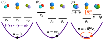
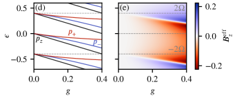
Figure 1: Model of atomic $p$-orbitals in a spherically symmetric harmonic potential. In the case where the potential is centered around zero (a), all levels in the $p$ shell are degenerate. Upon statically displacing the potential origin $\boldsymbol{u}=u\boldsymbol{e}_{x}$ (b), one of the three levels ($p_{x}$) changes its energy compared to the other levels ($p_{y}$, $p_{z}$). When the potential origin dynamically revolves around zero (c), i.e., $\boldsymbol{u}=u\hat{R}_{z}^{\Omega t}\boldsymbol{e}_{x}=u(\cos\Omega t,\sin\Omega t,0)^{T}$, the two levels in the rotation plane ($p_{x}$, $p_{y}$) experience Zeeman splitting, with the effective magnetic field $B_{z}^{\mathrm{eff}}$ depending on the rotation frequency $\Omega$ and the coupling strength $g$. The energy splitting in Floquet formalism, as a function of $g$ (in units where $u=1$) is depicted in panel (d), where we plot the Floquet eigenstates’ quasienergies and indicate the orbital polarization by color ($p_{z}$: black, $p_{+}$: red, $p_{-}$: blue). Panel (e) displays the energy dependent effective magnetic field obtained from projection of the (energy dependent) Floquet Hamiltonian on $l_{z}$ as a function of $g$. The pump frequency is set to $2\Omega=0.4$, as indicated by the dashed gray lines. Note that in panel (e), the energies refer to the physical energy scale, while in panel (d) we display Floquet quasienergies.

In principle, transfer of angular momentum from the nuclear to the electronic sector provides for an enhancement of the magnetic fields by a factor of $m_{n}/m_{e}\sim 10^{3}$ [21, 20]. Genuine magnetic fields might as well be amplified by momentum space topology of the electronic wave function [22, 23, 15]. In quantum mechanics, intrinsic magnetization can further arise from the inverse Faraday effect [24, 5, 25, 26, 13]. Pseudomagnetic fields, on the other hand, are known to exhibit enormous values for spatially inhomogeneous, static strain fields [27] and therefore pose another candidate for effective magnetic field enhancement. In this Letter, we show that driving nuclei on circular orbits can lead to pseudomagnetic fields of energy scales dictated by the electron-phonon coupling, translating to several tens of Teslas in perovskite crystals. These pseudomagnetic fields have their origin in quantum geometry of the electronic system on the manifold of nuclear coordinates.

Model. — To understand the origin of these pseudomagnetic fields we consider a simple spherically symmetric, quadratic Jahn-Teller model. Such a minimal model can be derived from a set of three degenerate electronic $p$ orbitals in a harmonic potential [see Fig. 1 (a)]. Expanding the potential $V(\boldsymbol{r})=k/2\,(\boldsymbol{r}-\boldsymbol{u})^{2}$ in the displacement $\boldsymbol{u}$, one obtains a linear term and an overall energy shift:

$$V(\boldsymbol{r})=\frac{k}{2}\boldsymbol{r}^{2}-k\boldsymbol{r}\cdot\boldsymbol{u}+\frac{k}{2}\boldsymbol{u}^{2}\,.$$ (1)

Negative parity of the $p$-states forbids first order perturbation theory contributions of the term $k\boldsymbol{r}\cdot\boldsymbol{u}$. Upon introduction of an $s$-like state at lower energies, we observe that a second-order contribution is symmetry-allowed and the perturbation in the $p$-electron sector becomes (for details see SM [17])

$$H^{(2)}_{ij} {}=g\braket{p_{i}}{\boldsymbol{r}\cdot\boldsymbol{u}}{s}\!\braket{s}{\boldsymbol{r}\cdot\boldsymbol{u}}{p_{j}}=gu_{i}u_{j}=g\big{[}\boldsymbol{u}^{2}-(\boldsymbol{l}\cdot\boldsymbol{u})^{2}\big{]}_{ij}$$ (2)

$${}=\mathrm{const.}-g\big{[}(\boldsymbol{l}\cdot\boldsymbol{u})^{2}\big{]}_{ij}\,,$$

where $\boldsymbol{l}$ is the orbital angular momentum operator and $g$ the coupling constant (we absorbed the norm of $\boldsymbol{u}$ into $g$ rendering $|\boldsymbol{u}|=1$). This effective Hamiltonian shifts the energy of the $p$ orbital along the $\boldsymbol{u}$ axis relative to the two other (real) $p$ orbitals [cf. Fig. 1 (b)]. We note that $H^{(2)}$ resembles a magnetic anisotropy of an $L=1$ angular momentum. If we now assume a periodically driven displacement, e.g., $\boldsymbol{u}=(\cos\Omega t,\sin\Omega t,0)^{T}$, we can treat the system in Floquet space. Following Refs. [28, 29, 30], we construct an effective Hamiltonian (in high-frequency or low-amplitude approximation) as

$$H^{\mathrm{eff}}=h_{0}+h_{2}\frac{1}{h_{0}-2\Omega}h_{2}^{\dagger}+h_{2}^{\dagger}\frac{1}{h_{0}+2\Omega}h_{2}\,,$$ (3)

where the Floquet hopping $h_{n}$ is defined as

$$h_{n}=\frac{1}{T}\int_{0}^{T}\!\!\mathrm{d}t\,e^{-in\Omega t}H^{(2)}\big{(}\boldsymbol{u}(t)\big{)}\,,$$ (4)

with $T=2\pi/\Omega$ the period of the drive. Note that all terms except $h_{0}$ and $h_{\pm 2}$ vanish due to the quadratic nature of $H^{(2)}$. We project  the effective Hamiltonian to the orbital angular momentum operators $\boldsymbol{l}$ and find

$$\boldsymbol{B}^{\mathrm{eff}}=\frac{\operatorname{\mathrm{Tr}}(H^{\mathrm{eff}}\boldsymbol{l})}{2}=\boldsymbol{e}_{z}B^{\mathrm{eff}}_{z}\,,\quad B^{\mathrm{eff}}_{z}=\frac{2\Omega g^{2}}{g^{2}-16\Omega^{2}}\,.$$ (5)

Apart from the effective magnetic field, $H^{\mathrm{eff}}$ induces dynamical crystal field splitting that discerns the $p_{z}$ orbital from the $p_{x}$ and $p_{y}$ orbitals. These properties are visualized in Fig. 1 (c), and a numerical calculation of the Floquet quasienergies is presented in panel (d). There, we additionally indicate the orbital polarization demonstrating how $B_{z}^{\mathrm{eff}}$ splits the $p_{\pm}$ sector. We note that in the antiadiabatic limit ($\Omega\gg g$), Eq. 5 predicts a quartic dependency of $B_{z}^{\mathrm{eff}}$ on the nuclear displacements $\boldsymbol{u}$: $B_{z}^{\mathrm{eff}}\propto g^{2}\propto\boldsymbol{u}^{4}$.

Floquet perturbation theory in the $\Omega\to\infty$ limit allows us to construct the eigenstates of the Floquet Hamiltonian [28]. Within this limit, we complement the above picture of an effective Hamiltonian with the quantum geometric one. The non-equilibrium analog to Berry’s phase for a state $\ket{\phi_{\alpha}(t)}$, the Aharonov-Anandan phase [32, 33, 29], is to leading order in $1/\Omega$ given as

$$\gamma^{\mathrm{AA}}_{\pm}=\int_{0}^{T}\!\!\mathrm{d}t\,\bra{\phi_{\pm}(t)}i\partial_{t}\ket{\phi_{\pm}(t)}=\pm\frac{\pi g^{2}}{4\Omega^{2}}$$ (6)

in the $p_{\pm}$ subspace. It enters the Floquet quasienergies as $\gamma^{\mathrm{AA}}_{\pm}/T$ and therefore generates the same $\Omega\to\infty$ result as the consideration through $H^{\mathrm{eff}}$:

$$\frac{\gamma^{\mathrm{AA}}_{-}}{T}=\frac{-g^{2}}{8\Omega}\sim\frac{2\Omega g^{2}}{g^{2}-16\Omega^{2}}\,,$$ (7)

therefore manifesting dynamical quantum geometry as the origin of the effective magnetic field in this maximally symmetric, quadratic Jahn-Teller model. Even for weak coupling strength $g\approx 10\,\mathrm{meV}$ and pump frequencies in the regime $\Omega\approx 20\,\mathrm{meV}\approx 5\,\mathrm{THz}$, the effective magnetic field reaches $B_{z}^{\mathrm{eff}}\approx 0.6\,\mathrm{meV}\approx\mu_{B}\,12\,\mathrm{T}$, which is expected to be larger when going beyond the high frequency limit.

Figure 1 (e) displays the numerical calculation of $B_{z}^{\mathrm{eff}}$ in the (molecular) spherical model Eq. 2. We obtain the energy dependency of the effective magnetic field from projecting the energy-dependent effective Hamiltonian to the angular momentum operators $\boldsymbol{l}$. This formulation extends Eq. 3 in that it takes all orders of $1/\Omega$ into account via inversion of the Floquet Green’s function’s $n=0$ block (cf. [30] and SM [17]), i.e., $H^{\mathrm{eff}}(\epsilon)=(\mathcal{G}(\epsilon)_{0,0})^{-1}$. In both panels (d) and (e), we set $\|\boldsymbol{u}\|=1$ and $\Omega=0.2$. The coupling strength $g$ therefore acts as an energy scale. We highlight that $B_{z}^{\mathrm{eff}}$ reaches values on the order of $g$ and $\Omega$.

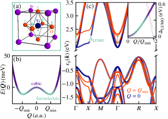
Figure 2: Electron-phonon coupling of the ferroelectric mode in SrTiO₃. Panel (a) displays the crystal structure in the cubic phase and additionally highlights the displacements of Ti and O atoms in the (unstable) ferroelectric phase (cyan arrows). In panel (b) we plot the energy $E(\boldsymbol{Q})$ of the electronic system as a function of the ferroelectric mode amplitude $Q$. Panel (c) presents the ab-initio electronic structure of SrTiO₃ in the cubic phase (thick blue lines, $Q=0$) and the ferroelectric phase (orange lines, $Q=Q_{\mathrm{min}}$). In the inset, we demonstrate the quadratic behavior of the valence band gap $\Delta_{\mathrm{LUMO}}$ as a function of the ferroelectric mode amplitude $Q/Q_{\mathrm{min}}$.

Material Realization. — The idealized spherical model as such might be difficult to realize in materials. The best discrete approximation of spherical symmetry is the icosahedral point group $I_{h}$. Buckyball fullerenes fall under this category—and with additional non-carbon atoms trapped in the graphene cages, so-called endofullerenes [34, 35, 36, 37] can host polar phonon modes at low energies. Strikingly, the main characteristics of the spherical model survive in environments with even lower point group symmetry. Suppose an octahedral ($O_{h}$) structure with (i) three degenerate $d$-orbital states in the $T_{2g}$ sector and (ii) three degenerate $T_{1u}$ optical phonon modes. Such systems are realized, e.g., in the conduction bands of crystals in the perovskite family. From symmetry analysis (see SM [17]), the quadratic Jahn-Teller Hamiltonian as a matrix in orbital space ($d_{yz}$, $d_{xz}$, $d_{xy}$) and as a function of phonon displacement $\boldsymbol{u}=(x,y,z)^{T}=\boldsymbol{u}(t)$ reads

$$H_{\mathrm{JT}}(t)=\gamma\boldsymbol{u}^{2}+\alpha\,\begin{pmatrix}\boldsymbol{u}^{2}-3x^{2}&\beta xy&\beta xz\\ \beta xy&\boldsymbol{u}^{2}-3y^{2}&\beta yz\\ \beta xz&\beta yz&\boldsymbol{u}^{2}-3z^{2}\end{pmatrix}\,.$$ (8)

To obtain meaningful values for $\alpha$ and $\beta$, we look at the polar optical $T_{1u}$ phonon modes in SrTiO₃. These modes are known to be controllable with terahertz radiation [38, 39, 9, 40] and strongly couple to the $T_{2g}$ electron sector: Figure 2 (c) displays the ab-initio band structure of SrTiO₃ in its symmetric coordination (blue) and under the influence of the polar $T_{1u}$ (ferroelectric) displacement (orange). A significant gap $\Delta_{\mathrm{LUMO}}$ at $\boldsymbol{k}=\Gamma$ opens when the atoms are displaced to the ferroelectric minimum $Q_{\mathrm{min}}$ (see inset). Panel (a) shows the real space displacements of the ferroelectric mode, where the titanium atoms move opposite to the oxygen octahedra creating a net polarization. At the ferroelectric minimum $Q_{\mathrm{min}}$, the titanium atoms are displaced by roughly $0.026\,\text{\AA}$ relative to the oxygen octahedra. We further show that the Higgs-like potential for the ferroelectric mode is shallow [see panel (b)], underlining that amplitudes on the order of the ferroelectric minimum $Q_{\mathrm{min}}$ can be reached by terahertz pumping [39, 9]. The values of $\alpha$ and $\beta$ [cf. Eq. 8] are adjusted by fitting the ab-initio gap sizes $\Delta_{\mathrm{LUMO}}$ at $\boldsymbol{k}=\Gamma$ to the eigenvalues of the Hamiltonian $H_{\mathrm{JT}}$ for a fine grid of displacement vectors $\boldsymbol{u}$. In units where $Q_{\mathrm{min}}=1$, we obtain $\alpha=6.55\cdot 10^{-2}\,\mathrm{eV}$ and $\beta=0.97$.

Using these parameters, Fig. 3 (a) demonstrates that rotation of the ferroelectric axis generates giant pseudomagnetic fields in the “molecular limit” (i.e., considering a single unit cell) of SrTiO₃ (with the rotation frequency set to $\Omega=0.02\,\mathrm{eV}\approx 5\,\mathrm{THz}$). Upon varying the coupling strength $\alpha$ (we fix $u=Q_{\mathrm{min}}\equiv 1$), we observe the same qualitative behavior as in the spherical model [cf. Fig. 1 (e)], rendering the influence of the symmetry reduction to $O_{h}$ minuscule. In reality, the $d$-electron block is strongly influenced by hopping of the electrons. Electron dispersion could lead to a significant reduction of the effective magnetic field given that their band width is approximately $1.5\,\mathrm{eV}$ [cf. Fig. 2 (c)] and only high-symmetry points are expected to contribute strongly to $B_{z}^{\mathrm{eff}}$. We incorporate the electron hopping into the Hamiltonian by adding

$$H_{\mathrm{kin}}=\operatorname{\mathrm{diag}}\begin{pmatrix}t_{2}\cos(k_{x})+t_{1}\cos(k_{y})+t_{1}\cos(k_{z})\\ t_{1}\cos(k_{x})+t_{2}\cos(k_{y})+t_{1}\cos(k_{z})\\ t_{1}\cos(k_{x})+t_{1}\cos(k_{y})+t_{2}\cos(k_{z})\\ \end{pmatrix}$$ (9)

as time independent part to the time dependent Hamiltonian Eq. 8, with $t_{1}=-0.34\,\mathrm{eV}$ and $t_{2}=-0.04\,\mathrm{eV}$ (obtained by simple fitting to the ab-initio band structure, see SM [17]). Subsequently we calculate the Floquet effective Hamiltonian at each $\boldsymbol{k}$-point in the Brillouin zone and sum up these contributions to form the local magnetic Hamiltonian $H_{\mathrm{mag}}$:

$$H_{\mathrm{mag}}(\epsilon)=\int\frac{\mathrm{d}\boldsymbol{k}}{V_{\mathrm{BZ}}}\,\big{(}\mathcal{G}(\boldsymbol{k},\epsilon)_{0,0}\big{)}^{-1}\,,$$ (10)

where $\mathcal{G}_{0,0}$ denotes the $n=0$ block of the Floquet Green’s function (for further details see SM [17]). We project $H_{\mathrm{mag}}$ to the orbital angular momentum operator and obtain the local effective magnetic field as $\boldsymbol{B}^{\mathrm{eff}}(\epsilon)=\operatorname{\mathrm{Tr}}[H_{\mathrm{mag}}(\epsilon)\boldsymbol{l}]/2$.

Figure 3: Effective magnetic field in conduction band sector of SrTiO₃ in (a) the molecular model and (b) the dispersive model that emerge upon periodic driving with $\Omega\approx 5\,\mathrm{THz}$ for varying electron-phonon coupling strength $\alpha$ [cf. Eq. 8]. The kinetic energy of the $d$ electrons substantially broadens the energy range $\epsilon$ in which significant effective magnetic fields $B_{z}^{\mathrm{eff}}$ are reached, while at the same time it smears away features present in the molecular limit (the conduction band edge is situated at $\epsilon=0$). Panel (c) displays the resultatnt Hall conductivity $\sigma_{H}$ from $p$-$d$ transitions across the band gap (that is modeled with $\Delta_{p\text{-}d}=3\,\mathrm{eV}$). Notably, nonzero values of $\sigma_{H}$ extend across the $d$-electron band width of approx. $1.5\,\mathrm{eV}$.

Figure 3 (b) shows that the local $B_{z}^{\mathrm{eff}}$ reaches values of roughly ten Tesla. Furthermore, most of the low energy structure visible in the molecular model [cf. Fig. 3 (a)] disappears upon inclusion of the electron dispersion.

In addition to the pseudomagnetic field generated by rotation of the ferroelectric mode, we calculate the $n=0$ Floquet optical conductivity [41, 42, 43] (homodyne component, i.e., “on-shell” response at the probe frequency) under the assumption of dipole transitions from a low-energy $p$-shell to the $T_{2g}$ electrons. Figure 3 (c) displays the resulting Hall conductivity $\sigma_{H}=\sigma_{xy}-\sigma_{yx}$ that has extended nonzero regions across the whole $T_{2g}$ electron band width. To calculate $\sigma_{H}$, we approximate the band gap of SrTiO₃ with $\Delta_{p\text{-}d}=3\,\mathrm{eV}$ and further neglect the electron-phonon coupling as well as the dispersion in the $p$-orbital sector (see Fig. 2 (c) and SM [17]).

Summary and discussion. — We propose a mechanism to obtain giant pseudomagnetic fields for electrons in both molecules and crystals. These fields are generated by the Aharonov-Anandan phase, a non-adiabatic extension to the concept of Berry’s phase, which the electron wave function collects through evolution along the trajectories of rotating nuclear degrees of freedom.

Through the example of a spherically symmetric quadratic Jahn-Teller model, we illustrate that the pseudomagnetic field strength is proportional to the inverse pump frequency $1/\Omega$ in the high-frequency limit. Even then, fields in the range of tens of Teslas are in reach for terahertz pump pulses. We further demonstrate that upon reducing the symmetry of the spherical model to $O_{h}$ and plugging in material parameters for the perovskite SrTiO₃, the resulting effective magnetic fields remain in the Tesla realm for pump frequencies in the intermediate frequency regime $\Omega\approx 5\,\mathrm{THz}$.

Such effective pseudomagnetic fields on the scale of several Teslas are by orders of magnitude bigger than magnetic fields from the phonon Zeeman and inverse Faraday effects. It it therefore tempting to compare our results to the experimental reports of dynamical multiferroicity [11] in SrTiO₃ by Basini et.al. [9]—the authors interpret the measured Kerr rotation in terms of effective magnetizations $\sim 0.1\,\mu_{B}\mathrm{T}/\mathrm{u.c.}$. This value for the apparent magnetization (via Kerr rotation) is smaller than the value of $B^{\mathrm{eff}}$ we obtain from the effective splitting, which is plausible for the following reasons: First, the $p$-orbital dispersion in the optical measurement will further smear out the Hall conductivity $\sigma_{H}$. Second, a measurement of $\sigma_{H}$ away from a resonance significantly reduces the pseudomagnetic field strength. Third, the phonon mode could be delocalized due to quantum nuclear effects, i.e., the average amplitude might only be a fraction of the ferroelectric minimum $Q_{\mathrm{min}}$ and also the phase will not be sharply defined.

According to Eq. 5, we expect a quartic dependence of $B_{z}^{\mathrm{eff}}$ on the driving electric field under the assumption of classical nuclei in a quadratic potential, which is at variance with the observations of a quadratic dependence by Basini et.al. [9]. Clearly, STO is a quantum paraelectric, where nuclear motion is governed by strong anharmonicities and quantum effects. These two effects demands further investigation in order to finally clarify whether in SrTiO₃, electron-nuclear quantum geometry can be seen as the source of dynamical multiferroicity [11, 38, 9, 44]. Apart from perovsikes close to ferroelectric phases [45, 9], we generically expect similar pseudomagnetic fields from electron-nuclear quantum geometry in materials with significant electron-phonon coupling of (polar) phonon modes to degenerate electronic levels, such as guest atoms in clathrate cages [46, 47, 48] or endofullerenes [34, 35, 36, 37]. Notably, the pseudomagnetic fields can be switched on ultrafast picosecond time scales.

Supplementary Information:
Ultrafast pseudomagnetic fields from electron-nuclear quantum geometry

S1 Circularly polarized phonons and Ampère’s law

We estimate an upper limit for the strength of magnetic fields generated by circularly polarized phonons by considering them as classically rotating charges. The magnetic moment of a single charge $q$ revolving at radius $r$ with frequency $\Omega$ is given as

$$\mu_{\mathrm{ph}}=I\,A=q\Omega\,\pi r^{2}\,,$$ (S1)

Assuming extreme conditions $q=2e$, $r=0.1\,\mathrm{\text{\AA}}$ and $\Omega/2\pi=6\,\mathrm{THz}$ as well as a very small unit cell of $V_{\mathrm{uc}}=5\,\mathrm{\text{\AA}^{3}}$, we obtain

$$B_{z}=\mu_{0}\,\frac{\mu_{\mathrm{ph}}}{V_{\mathrm{uc}}}\approx 1\,\mathrm{mT}\,.$$ (S2)

S2 The spherical model

To set up perturbation theory for $\boldsymbol{r}\cdot\boldsymbol{u}$, we must consider the expectation values of $\boldsymbol{r}$. Due to rotational invariance, it is sufficient to consider $r_{x}$:

$$\braket{p_{i}}{r_{x}}{p_{j}}\propto\int_{r<r_{\mathrm{max}}}\mathrm{d}^{3}\boldsymbol{r}~{}r_{i}r_{j}r_{x}=0\,,\quad\braket{p_{i}}{r_{x}}{s}\propto\int_{r<r_{\mathrm{max}}}\mathrm{d}^{3}\boldsymbol{r}~{}r_{i}r_{x}\propto\delta_{i,x}\,.$$ (S3)

It follows that $\braket{p_{i}}{\boldsymbol{r}}{s}\propto\boldsymbol{e}_{i}$ and therefore

$$H_{ij}^{(2)}=\tilde{g}\bra{p_{i}}\boldsymbol{r}\cdot\boldsymbol{u}\ket{s}\!\!\bra{s}\boldsymbol{r}\cdot\boldsymbol{u}\ket{p_{j}}=g\,(\boldsymbol{e}_{i}\cdot\boldsymbol{u})\,(\boldsymbol{e}_{j}\cdot\boldsymbol{u})=g\,u_{i}u_{j}\,,$$ (S4)

with $g$ and $\tilde{g}$ constants that allow us to absorb the energy denominator from second order perturbation theory. We wish to write Eq. S4 in a rotationally invariant form and make use of the fact that the squared angular momentum operators in $p$ orbital space span a basis of the diagonal components of (hermitian) operators acting on $p$ orbitals. The (squared) angular momentum operators read

$$l_{i}=i\varepsilon_{ijk}\ket{p_{j}}\!\!\bra{p_{k}}\,,\quad l_{i}^{2}=\mathbb{1}-\ket{p_{i}}\!\!\bra{p_{i}}\,.$$ (S5)

Due to rotational symmetry, we choose $\boldsymbol{u}$ to point in $\boldsymbol{e}_{x}$ direction without loss of generality. Equation S4 then becomes

$$H^{(2)} {}=\sum_{ij}H_{ij}^{(2)}\ket{p_{i}}\!\!\bra{p_{j}}=\sum_{ij}gu^{2}\,\delta_{i,x}\delta_{j,x}\ket{p_{i}}\!\!\bra{p_{j}}=gu^{2}\ket{p_{x}}\!\!\bra{p_{x}}=gu^{2}\big{(}\mathbb{1}-l_{x}^{2}\big{)}$$ (S6)

$${}=g\boldsymbol{u}^{2}-g\big{(}\boldsymbol{u}\cdot\boldsymbol{l}\big{)}^{2}\,,$$

with the second line being the basis independent way of writing $H^{(2)}$, and thus the one that can be applied for arbitrary $\boldsymbol{u}$.

S3 Floquet perturbation theory of the spherical model

The Hamiltonian for the spherical quadratic Jahn-Teller model (cf. Eq. 2 of the main text) reads

$$H^{(2)}=-g(\boldsymbol{u}\cdot\boldsymbol{l})^{2}=-g\begin{pmatrix}\boldsymbol{u}^{2}-x^{2}&xy&xz\\ xy&\boldsymbol{u}^{2}-y^{2}&yz\\ xz&yz&\boldsymbol{u}^{2}-z^{2}\\ \end{pmatrix}\,,$$ (S7)

with the basis states $\ket{p_{x}}$, $\ket{p_{y}}$, $\ket{p_{z}}$. Since it is spherically symmetric, we choose to rotate with $\boldsymbol{\Omega}\parallel\boldsymbol{e}_{z}$, i.e.,

$$\boldsymbol{u}(t)=\begin{pmatrix}\cos(\Omega t)\\ \sin(\Omega t)\\ 0\end{pmatrix}\,.$$ (S8)

The resulting time-dependent Hamiltonian reads

$$H^{(2)}(t)=-g\begin{pmatrix}1-\cos^{2}(\Omega t)&\cos(\Omega t)\sin(\Omega t)&0\\ \cos(\Omega t)\sin(\Omega t)&1-\sin^{2}(\Omega t)&0\\ 0&0&1\\ \end{pmatrix}\,.$$ (S9)

In Floquet space, we determine the “hoppings” as

$$h_{n}=\frac{1}{T}\int_{0}^{T}\!\!\mathrm{d}t\,e^{-in\Omega t}\,H^{(2)}(t)=-g\begin{cases}\operatorname{\mathrm{diag}}(1/2,1/2,1)&\text{for}~{}n=0\\ -\sigma_{z}/4\pm i\sigma_{x}/4&\text{for}~{}n=\pm 2\\ 0&\text{else}\end{cases}\,,\quad\text{with}~{}\sigma_{z}=\begin{pmatrix}1&0&0\\ 0&-1&0\\ 0&0&0\\ \end{pmatrix}\,,\quad\sigma_{x}=\begin{pmatrix}0&1&0\\ 1&0&0\\ 0&0&0\\ \end{pmatrix}\,.$$ (S10)

Since only zeroth and second order terms contribute, we can treat Floquet space in terms of $2\Omega$. The Floquet Hamiltonian therefore can be represented in matrix form as

$$H_{F}=\begin{pmatrix}\ddots&h_{2}\\ h_{2}^{\dagger}&h_{0}+4\Omega&h_{2}\\ &h_{2}^{\dagger}&h_{0}+2\Omega&h_{2}\\ &&h_{2}^{\dagger}&h_{0}&h_{2}\\ &&&h_{2}^{\dagger}&h_{0}-2\Omega&h_{2}\\ &&&&h_{2}^{\dagger}&h_{0}-4\Omega&h_{2}\\ &&&&&h_{2}^{\dagger}&\ddots\\ \end{pmatrix}\,.$$ (S11)

The high-frequency perturbation theory [28] for the $\ket{p_{\pm}}=1/\sqrt{2}\big{(}\ket{p_{x}}\pm i\ket{p_{y}}\big{)}$ states becomes

$$\ket{p_{\pm}^{(1)}(t)}=\sum_{n\neq 0}\frac{h_{-n}\,e^{in\Omega t}}{n\Omega}\ket{p_{\pm}}=\bigg{(}\frac{h_{2}e^{-i2\Omega t}}{-2\Omega}+\frac{h_{-2}e^{i2\Omega t}}{2\Omega}\bigg{)}\ket{p_{\pm}}\,.$$ (S12)

From this expression, we can calculate the Aharonov-Anandan phase [32, 33, 29] as

$$\frac{\gamma^{\mathrm{AA}}_{\pm}}{T}=\frac{1}{T}\int_{0}^{T}\mathrm{d}t\braket{p_{\pm}^{(1)}(t)}{i\partial_{t}}{p_{\pm}^{(1)}(t)}=\bra{p_{\pm}}\bigg{(}\frac{1}{2\Omega}\big{[}h_{2}^{\dagger},h_{2}\big{]}\bigg{)}\ket{p_{\pm}}=\pm\frac{g^{2}}{8\Omega}\,.$$ (S13)

As we shall see below, it perfectly coincides with the magnetic fields generated in the effective Hamiltonian picture.

S4 Floquet Green’s functions and effective Hamiltonians

The resolvent operator in Floquet space can be defined as the matrix inverse of $H_{F}$ [cf. Eq. S11]:

$$\mathcal{G}(\omega)=\frac{1}{\omega-H_{F}}\,.$$ (S14)

We define the effective Hamiltonian as the re-inversion of the $n=0$ Floquet block of $\mathcal{G}$, i.e.,

$$H^{\mathrm{eff}}(\omega)=\big{(}\mathcal{G}_{0,0}(\omega)\big{)}^{-1}\,.$$ (S15)

This creates, in addition to the time-averaged Hamiltonian $h_{0}$, self-energy like terms that, upon inversion, yield the correct propagator. In order to circumvent points where $\mathcal{G}_{0,0}$ is not invertible, we add an imagniary broadening to $\omega$, i.e., $\omega\leftarrow\omega+i\eta$ with $\eta=2\cdot 10^{-2}\,\mathrm{eV}$. To leading order in $1/\Omega$ and for $\omega=0$, we can express $H^{\mathrm{eff}}$ as

$$H^{\mathrm{eff}}=h_{0}+h_{2}\,\frac{1}{h_{0}-2\Omega}\,h_{2}^{\dagger}+h_{2}^{\dagger}\,\frac{1}{h_{0}+2\Omega}\,h_{2}\,,$$ (S16)

i.e., propagating to the next Floquet block and back. For the spherical model, we construct $H^{\mathrm{eff}}$ explicitly and project it to the orbital angular momentum operator $l_{z}$:

$$h_{2}\frac{1}{h_{0}\pm 2\Omega}h_{2}^{\dagger} {}=\frac{g^{2}}{16}\,(\sigma_{z}\mp i\sigma_{x})\,\frac{1}{g/2\pm 2\Omega}\,(\sigma_{z}\pm i\sigma_{x})=\frac{g^{2}}{8g\pm 32\Omega}(\sigma_{z}^{2}+\sigma_{x}^{2}\pm i\sigma_{z}\sigma_{x}\mp i\sigma_{x}\sigma_{z})$$ (S17)

$${}=\frac{g^{2}}{4g\pm 16\Omega}(\mathbb{1}\pm\sigma_{y})\,,$$

$$B^{\mathrm{eff}}_{z}=\frac{\operatorname{\mathrm{Tr}}(l_{z}H^{\mathrm{eff}})}{2} {}=\frac{\operatorname{\mathrm{Tr}}(\sigma_{y}H^{\mathrm{eff}})}{2}=\frac{g^{2}}{4g-16\Omega}-\frac{g^{2}}{4g+16\Omega}=\frac{g^{2}(4g+16\Omega)-g^{2}(4g-16\Omega)}{(4g)^{2}-(16\Omega)^{2}}=\frac{2g^{2}\Omega}{g^{2}-16\Omega^{2}}\,.$$ (S18)

Note that we restricted ourselves to the two-dimensional $\ket{p_{x,y}}$ subspace, as $h_{2}$ limits us to contributions in that sector.

In addition to the molecular picture above, we also perform calculations for periodic systems. In general, $H^{\mathrm{eff}}$ then becomes a $\boldsymbol{k}$-dependent quantity, as the Green’s function is diagonal in $\boldsymbol{k}$:

$$\mathcal{G}(\boldsymbol{k},\omega)=\frac{1}{\omega-H_{F}(\boldsymbol{k})}\,,$$ (S19)

where in our case $H_{F}(\boldsymbol{k})_{m,n}=(H_{F})_{m,n}+H(\boldsymbol{k})\delta_{m,n}$. For controlling local degrees of freedom, i.e., orbitals, it is useful to calculate an average (local) effective Hamiltonian. Brillouin zone integration yields something very similar to density of states broadening, i.e.,

$$H^{\mathrm{eff}}=\int\frac{\mathrm{d}\boldsymbol{k}}{V_{\mathrm{BZ}}}\,\big{(}\mathcal{G}_{0,0}(\boldsymbol{k},\omega)\big{)}^{-1}\,.$$ (S20)

On this effective Hamiltonian, we can apply the same tracing procedure as above ($B_{z}^{\mathrm{eff}}=\operatorname{\mathrm{Tr}}[H^{\mathrm{eff}}l_{z}]/2$) to get the effective magnetic field. In numerical simulations, we size the momentum mesh as to contain $80^{3}$ regularly spaced points in the BZ.

S5 The quadratic $T_{2g}\otimes T_{1u}$ Jahn-Teller model

To go beyond the spherical model, we deduct the quadratic Jahn-Teller model of electronic states in the $T_{2g}$ irreducible representation (irrep) coupled to phonon modes in the $T_{1u}$ irrep (of the $O_{h}$ point group). We first note that the electronic space can be decomposed into

$$T_{2g}\otimes T_{2g}=A_{1g}\oplus E_{g}\oplus T_{1g}\oplus T_{2g}\,.$$ (S21)

Furthermore, we find that the product of two $T_{1u}$ modes yields the same decomposition, i.e., $T_{1u}\otimes T_{1u}=T_{2g}\otimes T_{2g}$. As the overall Jahn-Teller Hamiltonian must be a scalar (transform in $A_{1g}$), only direct products of identical irreps contribute. To determine their prefactors, we carried out Clebsch-Gordon decompositions (using GTPack [50, 51]) and arrived at:

$$H_{\mathrm{JT}}=\alpha^{A_{1g}}\,H_{\mathrm{el}}^{A_{1g}}C_{\mathrm{ph}}^{A_{1g}}+\alpha^{E_{g}}\,\frac{1}{\sqrt{2}}\Big{(}H_{\mathrm{el}}^{E_{g};1}C_{\mathrm{ph}}^{E_{g};1}+H_{\mathrm{el}}^{E_{g};2}C_{\mathrm{ph}}^{E_{g};2}\Big{)}+\alpha^{T_{2g}}\frac{1}{\sqrt{3}}\sum_{i=1}^{3}H_{\mathrm{el}}^{T_{2g};i}C_{\mathrm{ph}}^{T_{2g};i}+\alpha^{T_{1g}}\frac{1}{\sqrt{3}}\sum_{i=1}^{3}H_{\mathrm{el}}^{T_{1g};i}C_{\mathrm{ph}}^{T_{1g};i}\,.$$ (S22)

The electron (phonon) Hamiltonians $H^{\mathrm{irrep}}_{\mathrm{el}}$ ($C^{\mathrm{irrep}}_{\mathrm{ph}}$) are tabulated in Table SI.

Table SI: Table of quadratic Hamiltonian contributions in different irreducible representations for electrons in the $T_{2g}$ and phonons in the $T_{1u}$ block. Each row contains a contribution to an irrep, with the first column labeling the irrep, the second column corresponding to the electronic Hamiltonian contribution $H_{\mathrm{el}}^{\mathrm{irrep}}$ and the third one to the phononic one; $C_{\mathrm{ph}}^{\mathrm{irrep}}$. We label the electronic states as $\ket{1}=\ket{p_{x}}$, $\ket{2}=\ket{p_{y}}$, $\ket{3}=\ket{p_{z}}$.

irrep	$H^{\mathrm{irrep}}_{\mathrm{el}}$	$C_{\mathrm{ph}}^{\mathrm{irrep}}$
$A_{1g}$	$\mathbb{1}$	$x^{2}+y^{2}+z^{2}$
$E_{g};1$	$1/\sqrt{2}\,\big{(}-\ket{1}\!\!\bra{1}+\ket{3}\!\!\bra{3}\big{)}$	$1/\sqrt{2}\,\big{(}z^{2}-x^{2}\big{)}$
$E_{g};2$	$1/\sqrt{3}\,\big{(}\sqrt{2}\ket{2}\!\!\bra{2}-\ket{1}\!\!\bra{1}/\sqrt{2}-\ket{3}\!\!\bra{3}/\sqrt{2}\big{)}$	$1/\sqrt{3}\,\big{(}x^{2}/\sqrt{2}-\sqrt{2}y^{2}+z^{2}/\sqrt{2}\big{)}$
$T_{1g};1$	$\ket{2}\!\!\bra{1}-\ket{1}\!\!\bra{2}$	$0$
$T_{1g};2$	$\ket{2}\!\!\bra{3}-\ket{3}\!\!\bra{2}$	$0$
$T_{1g};3$	$\ket{1}\!\!\bra{3}-\ket{3}\!\!\bra{1}$	$0$
$T_{2g};1$	$\ket{2}\!\!\bra{1}+\ket{1}\!\!\bra{2}$	$xy$
$T_{2g};2$	$\ket{3}\!\!\bra{2}+\ket{2}\!\!\bra{3}$	$yz$
$T_{2g};3$	$\ket{1}\!\!\bra{3}+\ket{3}\!\!\bra{1}$	$xz$

After collecting all the terms and simplifying, one arrives at

$$H_{\mathrm{tot}} \begin{aligned} &{}=\alpha_{1}\,\frac{x^{2}+y^{2}+z^{2}}{3}\begin{pmatrix}1&0&0\\ 0&1&0\\ 0&0&1\end{pmatrix}+\alpha_{2}\,\frac{z^{2}-x^{2}}{2\sqrt{2}}\begin{pmatrix}-1&0&0\\ 0&0&0\\ 0&0&1\end{pmatrix}+\alpha_{2}\,\frac{x^{2}-2y^{2}+z^{2}}{6\sqrt{2}}\begin{pmatrix}-1&0&0\\ 0&2&0\\ 0&0&-1\end{pmatrix}+{}\\ &\phantom{{}={}}\alpha_{3}\,\frac{yz}{\sqrt{3}}\begin{pmatrix}0&0&0\\ 0&0&1\\ 0&1&0\end{pmatrix}+\alpha_{3}\,\frac{xz}{\sqrt{3}}\begin{pmatrix}0&0&1\\ 0&0&0\\ 1&0&0\end{pmatrix}+\alpha_{3}\,\frac{xy}{\sqrt{3}}\begin{pmatrix}0&1&0\\ 1&0&0\\ 0&0&0\end{pmatrix}\\ &{}=\gamma\boldsymbol{u}^{2}+\alpha\,\begin{pmatrix}\boldsymbol{u}^{2}-3x^{2}&\beta xy&\beta xz\\ \beta xy&\boldsymbol{u}^{2}-3y^{2}&\beta yz\\ \beta xz&\beta yz&\boldsymbol{u}^{2}-3z^{2}\end{pmatrix}\,.\end{aligned}$$ (S23)

After dropping contributions proportional to $\mathbb{1}$ one can verify that Eq. 8 is obtained. We further note that the quadratic $T_{2g}\otimes T_{1u}$ Jahn-Teller Hamiltonian $H_{\mathrm{JT}}$ in fact only differs from the spherical model $H^{(2)}$ by the factor $\beta$, when the amplitude $\|\boldsymbol{u}\|$ is assumed constant—for $\beta=3$, we recover all nontrivial terms.

Notably, the hopping matrix elements in an electronic Hamiltonian can be derived in a similar manner. Close to $\boldsymbol{k}=\Gamma$, we assume a quadratic dependency on momenta $\boldsymbol{k}$, rendering the symmetry analysis equivalent to the one above. On the diagonal, therefore obtain

$$H_{\mathrm{kin}}\approx\operatorname{\mathrm{diag}}\begin{pmatrix}A\boldsymbol{k}^{2}+Bk_{x}^{2}\\ A\boldsymbol{k}^{2}+Bk_{y}^{2}\\ A\boldsymbol{k}^{2}+Bk_{z}^{2}\\ \end{pmatrix}\to\operatorname{\mathrm{diag}}\begin{pmatrix}t_{2}\cos k_{x}+t_{1}\cos k_{y}+t_{1}\cos k_{z}\\ t_{1}\cos k_{x}+t_{2}\cos k_{y}+t_{1}\cos k_{z}\\ t_{1}\cos k_{x}+t_{1}\cos k_{y}+t_{2}\cos k_{z}\\ \end{pmatrix}\,,$$ (S24)

where we identify $A=\gamma+\alpha$ and $B=-3\alpha$. This diagonal $T_{2g}$ Hamiltonian is the one from Eq. 9 of the main text.

S6 ab-initio parameters for SrTiO₃

All Density Functional (Perturbation) Theory calculations are carried out using Quantum ESPRESSO [52, 53]. For the transformation of the electronic energies and electron-phonon couplings to the Wannier basis, we use Wannier90 [54] and the EPW code [55, 56]. We have applied the Perdew-Burke-Ernzerhof (PBE) functional [57] in combination with Ultrasoft pseudopotentials [58] from the SSSP library [59, 60]. Furthermore, we used a lattice constant of 3.936 Å, set the plane-wave cutoff to 120 Ry and used $4\times 4\times 4$ points for both the $\boldsymbol{k}$ and the $\boldsymbol{q}$ meshes.

To fit the parameters for the quadratic electron phonon-coupling at the $\Gamma$-point using Eq. 8 of the main text, we use a $8\times 8\times 8$ mesh of displacements from $Q_{x,y,z}\in\{0,\dots,Q_{\mathrm{min}}\}$. One eighth of the full cube is sufficient due to $O_{h}$ symmetry.

We show the fit of $H_{\mathrm{kin}}$ to the electronic band structure obtained from DFT in Fig. S1.

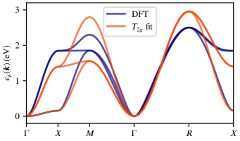
Figure S1: Fit of the diagonal $T_{2g}$ Hamiltonian Eq. S24 to the DFT band structure (cf. Fig. 2 (c) of the main text). The resulting parameters are $t_{1}=-0.34\,\mathrm{eV}$ and $t_{2}=-0.04\,\mathrm{eV}$. For quantitative agreement with the features at higher energies, one would need to include further ranged- as well as off-diagonal hopping parameters.

S7 Floquet optical conductivity

The optical response function in Floquet theory can be written as [33, 41, 42]

$$\sigma_{\mu\nu}^{(n)}=\frac{i}{\omega}\sum_{\alpha}f_{\alpha}\langle\langle\phi_{\alpha,0}|j_{\mu}\mathcal{G}(\omega+\epsilon_{\alpha}+n\Omega)j_{\nu}+j_{\nu}\mathcal{G}^{\dagger}(-\omega+\epsilon_{\alpha})j_{\mu}|\phi_{\alpha,n}\rangle\rangle\,,$$ (S25)

where the index $n$ corresponds to responses at frequency $\omega+n\Omega$ and we omit the diamagnetic contribution. We use the following notation for the Floquet expectation value of an operator $\mathcal{O}$:

$$\langle\langle\phi_{\alpha,n}|\mathcal{O}|\phi_{\beta,m}\rangle\rangle=\frac{1}{T}\int_{0}^{T}\!\!\mathrm{d}t\,\braket{\phi_{\alpha,n}(t)}{\mathcal{O}}{\phi_{\beta,m}(t)}\,,$$ (S26)

with $\ket{\phi_{\alpha,n}(t)}$ being the $n$-th Floquet block of the Floquet state $\alpha$. We here restrict ourselves to considering the $n=0$ component of $\sigma^{(n)}$ [Eq. S25], i.e. the so-called homodyne component. In addition, we use dipole operators instead of current operators, i.e., we make the substitution $j_{\mu}=\partial_{t}d_{\mu}=-i\omega d_{\mu}$. This simplification is made possible because are interested in interband transitions from the valence states to the conduction band and not in how momentum space itself affects the optical transitions.

The occupation therefore is $f_{\alpha}=0$ for conduction bands and $f_{\alpha}=1$ for valence bands. As the dipole operators don’t change Floquet indices, Eq. S25 is simplified through the insertion of a one as follows:

$$\sigma_{\mu\nu} {}\equiv\sigma^{(0)}_{\mu\nu}=i\omega\sum_{\alpha\in\mathrm{valence}}\sum_{\beta,n}\big{[}\langle\langle\phi_{\alpha,0}|d_{\mu}\mathcal{G}(\omega+\epsilon_{\alpha})|\phi_{\beta,n}\rangle\rangle\langle\langle\phi_{\beta,n}|d_{\nu}|\phi_{\alpha,0}\rangle\rangle+\langle\langle\phi_{\alpha,0}|d_{\nu}\mathcal{G}^{\dagger}(-\omega+\epsilon_{\alpha})|\phi_{\beta,n}\rangle\rangle\langle\langle\phi_{\beta,n}|d_{\mu}|\phi_{\alpha,0}\rangle\rangle\big{]}$$ (S27)

$${}=i\omega\sum_{\alpha\in\mathrm{valence}}\sum_{\beta}\big{[}\langle\langle\phi_{\alpha,0}|d_{\mu}\mathcal{G}(\omega+\epsilon_{\alpha})|\phi_{\beta,0}\rangle\rangle\langle\langle\phi_{\beta,0}|d_{\nu}|\phi_{\alpha,0}\rangle\rangle+\langle\langle\phi_{\alpha,0}|d_{\nu}\mathcal{G}^{\dagger}(-\omega+\epsilon_{\alpha})|\phi_{\beta,0}\rangle\rangle\langle\langle\phi_{\beta,0}|d_{\mu}|\phi_{\alpha,0}\rangle\rangle\big{]}$$

$${}=i\omega\sum_{\alpha\in\mathrm{valence}}\operatorname{\mathrm{Tr}}\big{[}d_{\nu}|\phi_{\alpha,0}\rangle\rangle\langle\langle\phi_{\alpha,0}|d_{\mu}\mathcal{G}_{0,0}(\omega+\epsilon_{\alpha})+d_{\mu}|\phi_{\alpha,0}\rangle\rangle\langle\langle\phi_{\alpha,0}|d_{\nu}\mathcal{G}_{0,0}^{\dagger}(-\omega+\epsilon_{\alpha})\big{]}$$

$${}=i\omega\sum_{i\in\{x,y,z\}}\operatorname{\mathrm{Tr}}\big{[}d_{\nu}\ket{p_{i}}\!\!\bra{p_{i}}d_{\mu}\mathcal{G}_{0,0}(\omega+\epsilon_{p})+d_{\mu}\ket{p_{i}}\!\!\bra{p_{i}}d_{\nu}\mathcal{G}^{\dagger}_{0,0}(-\omega+\epsilon_{p})\big{]}\,,$$

with the trace extending over all conduction band $n=0$ states. The dipole operators in $p$-orbital and $d$-orbital space read

$$\mathsf{d}_{x}=\begin{pmatrix}0&0&0\\ 0&0&1\\ 0&1&0\\ \end{pmatrix}\,,\quad\mathsf{d}_{y}=\begin{pmatrix}0&0&1\\ 0&0&0\\ 1&0&0\\ \end{pmatrix}\,,\quad\mathsf{d}_{z}=\begin{pmatrix}0&1&0\\ 1&0&0\\ 0&0&0\\ \end{pmatrix}\,,$$ (S28)

where rows correspond to $p_{x},p_{y},p_{z}$ and columns to $d_{yz},d_{xz},d_{xy}$. The products of dipole operators over the $p$ subspace the last line of Eq. S27 are constructed as matrix multiplications of the above operators and their transpose, i.e.,

$$\sum_{i\in\{x,y,z\}}d_{\nu}\ket{p_{i}}\!\!\bra{p_{i}}d_{\mu}=\mathsf{d}_{\nu}^{T}\mathsf{d}_{\mu}\,.$$ (S29)

Notably, the off-diagonal combinations (in $\mu,\nu$) of those matrix products correspond to entries of the orbital angular momentum operator (in the $d$ orbitals):

$$\mathsf{d}_{x}^{T}\mathsf{d}_{y}-\mathsf{d}_{y}^{T}\mathsf{d}_{x}=\begin{pmatrix}0&-1&0\\ 1&0&0\\ 0&0&0\end{pmatrix}=i\,l_{z}=i\,\begin{pmatrix}0&i&0\\ -i&0&0\\ 0&0&0\end{pmatrix}\,.$$ (S30)

As we assume a flat valence band manifold, i.e., $\epsilon_{p}\equiv\mathrm{const.}$, Eq. S27 becomes

$$\sigma_{\mu\nu}=i\omega\operatorname{\mathrm{Tr}}\big{[}\mathsf{d}_{\nu}^{T}\mathsf{d}_{\mu}\mathcal{G}_{0,0}(\omega+\epsilon_{p})+\mathsf{d}_{\mu}^{T}\mathsf{d}_{\nu}\mathcal{G}_{0,0}^{\dagger}(-\omega+\epsilon_{p})\big{]}\,.$$ (S31)

When we consider the Hall conductivity, we observe how the relation to the orbital angular momentum operator Eq. S30 enters:

$$\sigma_{H}^{z}=\sigma_{xy}-\sigma_{yx}=\omega\operatorname{\mathrm{Tr}}\big{[}l_{z}\big{(}\mathcal{G}_{0,0}(\omega+\epsilon_{p})-\mathcal{G}_{0,0}(-\omega+\epsilon_{p})\big{)}\big{]}\,.$$ (S32)

Lastly, we note that we can simplify Eq. S31 by decomposing the conduction band manifold trace into an orbital contribution and a momentum one to yield

$$\sigma_{\mu\nu}=i\omega\int\frac{\mathrm{d}\boldsymbol{k}}{V_{\mathrm{BZ}}}\operatorname{\mathrm{Tr}}\big{[}\mathsf{d}_{\nu}^{T}\mathsf{d}_{\mu}\mathcal{G}_{(0,0)}(\boldsymbol{k},\omega+\epsilon_{p})+\mathsf{d}_{\mu}^{T}\mathsf{d}_{\nu}\mathcal{G}^{\dagger}_{(0,0)}(\boldsymbol{k},-\omega+\epsilon_{p})\big{]}\,.$$ (S33)

Equation S33 is what we numerically implement to obtain the spectrum in Fig. 3 (b) of the main text. Note that as in Section S4, we must employ spectral broadening $i\eta=i\,2\cdot 10^{-2}\,\mathrm{eV}$ in order to smoothen poles; and the momentum resolution is $160^{3}$ points on a regular grid. We furthermore set $\epsilon_{p}=-3\,\mathrm{eV}$, roughly corresponding to the band gap of SrTiO₃.

Supplementary References

• T. Oka and S. Kitamura, Floquet Engineering of Quantum Materials, Annual Review of Condensed Matter Physics 10, 387 (2019)

• Y. Aharonov and J. Anandan, Phase change during a cyclic quantum evolution, Physical Review Letters 58, 1593 (1987)

• T. Oka and H. Aoki, Photovoltaic Hall effect in graphene, Physical Review B 79, 081406 (2009)

• A. Kumar, M. Rodriguez-Vega, T. Pereg-Barnea, and B. Seradjeh, Linear response theory and optical conductivity of Floquet topological insulators, Physical Review B 101, 174314 (2020)

• A. Cupo, J. T. Heath, E. Cobanera, J. D. Whitfield, C. Ramanathan, and L. Viola, Optical conductivity signatures of Floquet electronic phases, Physical Review B 108, 024308 (2023)

• R. M. Geilhufe and W. Hergert, GTPack: A Mathematica Group Theory Package for Application in Solid-State Physics and Photonics, Frontiers in Physics 6, 86 (2018)

• W. Hergert and R. M. Geilhufe, Group Theory in Solid State Physics and Photonics: Problem Solving with Mathematica (Wiley-VCH, 2018) isbn: 978-3-527-41133-7

• P. Giannozzi et al., Quantum ESPRESSO: A modular and open-source software project for quantum simulations of materials, J. Phys. Condens. Matter 21, 395502 (2009), arXiv:0906.2569

• P. Giannozzi et al., Advanced capabilities for materials modelling with Quantum ESPRESSO, J. Phys. Condens. Matter 29, 465901 (2017), arXiv:1709.10010

• A. A. Mostofi, J. R. Yates, G. Pizzi, Y.-S. Lee, I. Souza, D. Vanderbilt, and N. Marzari, An updated version of wannier90: A tool for obtaining maximally-localised Wannier functions, Comput. Phys. Commun. 185, 2309 (2014)

• J. Noffsinger, F. Giustino, B. D. Malone, C.-H. Park, S. G. Louie, and M. L. Cohen, EPW: A program for calculating the electron–phonon coupling using maximally localized Wannier functions, Comput. Phys. Commun. 181, 2140 (2010), arXiv:1005.4418

• S. Poncé, E. Margine, C. Verdi, and F. Giustino, EPW: Electron–phonon coupling, transport and superconducting properties using maximally localized Wannier functions, Comput. Phys. Commun. 209, 116 (2016), arXiv:1604.03525

• J. P. Perdew, K. Burke, and M. Ernzerhof, Generalized gradient approximation made simple, Phys. Rev. Lett. 77, 3865 (1996)

• D. Vanderbilt, Soft self-consistent pseudopotentials in a generalized eigenvalue formalism, Phys. Rev. B 41, 7892 (1990)

• G. Prandini, A. Marrazzo, I. E. Castelli, N. Mounet, and N. Marzari, Precision and efficiency in solid-state pseudopotential calculations, npj Comput. Mater. 4, 1 (2018), arXiv:1806.05609

• G. Prandini, A. Marrazzo, I. E. Castelli, N. Mounet, E. Passaro, and N. Marzari, A standard solid state pseudopotentials (SSSP) library optimized for precision and efficiency, Materials Cloud Archive 2021.76, 10.24435/materialscloud:rz-77 (2021)