Aligned Yet Large Dipoles: a SMEFT Study

Abstract

We study a non-universal flavor scenario at the level of the Standard Model Effective Field Theory, according to which the matrix of Wilson coefficients $c_{uW}$ of an up-type electroweak quark dipole operator is aligned with the up-type Yukawa coupling. Such an alignment usually follows from the assumption of Minimal Flavor Violation (MFV), away from which we step by allowing the entries of $c_{uW}$ to be sizable along the first quark generations. A particular example, which we refer to as “inverse hierarchy MFV”, features Wilson coefficients inversely proportional to quark masses, and arises from BSM models respecting MFV and containing heavy fields that replicate the mass hierarchy of SM quarks. We then analyze the phenomenology driven by $c_{uW}$ at colliders and at lower-energy flavor experiments. We show that precision measurements of the process $pp\rightarrow Wh\rightarrow\gamma\gamma\ell\nu$ at FCC-$hh$ could set an upper bound on $|c_{uW}|\lesssim\mathcal{O}(10^{-2})(\Lambda/\text{TeV})^{2}$, with $\Lambda$ the cutoff of the effective field theory. This bound is an order of magnitude stronger than the existing LHC bounds. Moreover, we estimate that $Wh\rightarrow b\bar{b}\ell\nu$ at HL-LHC could also give competitive bounds. In the low-energy regime, we consider bounds arising from rare kaon decays, which turn out to be loose, $|c_{uW}^{11}|<\mathcal{O}(1)(\Lambda/\text{TeV})^{2}$. We finally demonstrate that our flavor and operator assumptions can be derived from a weakly-coupled UV model, which we choose to simultaneously illustrate the UV origin of inverse hierarchy MFV.

1 Introduction

New high-energy physics (NP), which is expected for several compelling, theoretical and observational reasons, could manifest itself in a variety of ways. Under the assumption that it couples significantly to the Standard Model (SM) degrees of freedom, two main scenarios have been considered: the new particles are light enough to be produced at colliders, or they are too heavy. In the latter case, NP models can be matched onto effective field theories (EFTs), which can often be taken to be the Standard Model Effective Field Theory (SMEFT) Buchmuller:1985jz ; Grzadkowski:2010es ; Murphy:2020rsh ; Li:2020gnx ; Li:2020xlh ; Harlander:2023psl (see Alonso:2015fsp ; Falkowski:2019tft ; Cohen:2020xca for exceptions), whose cutoff corresponds to the scale of NP.

Taken at face value, the SMEFT has, already at dimension-6 order, a great number of free parameters. Although one may consider all parts of this parameter space as equally probable up to theoretical constraints on its physical region (see e.g.,  Arzt:1994gp ; Einhorn:2013kja ; Craig:2019wmo ; Adams:2006sv ; Zhang:2018shp ; Remmen:2019cyz ; Zhang:2020jyn ), the properties of the SM and many experimental measurements suggest that NP has a highly non-trivial structure. This is especially true in the flavor sector, where the existence of three generations of matter, together with the very hierarchical quark masses and mixings, suggest that a mechanism is at play at higher energies. Different foundational paradigms have been proposed in that direction, which require for instance new family-dependent “horizontal” broken symmetries Froggatt:1978nt ; Leurer:1992wg ; Leurer:1993gy , extra dimensions of space Arkani-Hamed:1999ylh ; Grossman:1999ra ; Dvali:2000ha ; Gherghetta:2000qt ; Huber:2000ie or SM couplings to a strong sector that generate strongly hierarchical fermion kinetic terms Nelson:2000sn ; Davidson:2007si . All those constructions predict very strong hierarchies in the flavored coefficients of the SMEFT Isidori:2009px ; Efrati:2015eaa ; Aharony:2010ch ; Csaki:2009wc ; Bordone:2019uzc ; Faroughy:2020ina ; Greljo:2022cah which, for the physicist interested in producing the associated new particles in experiments, is very fortunate: were the flavored SMEFT coefficients random, they would impose bounds on the scale of NP (or, to be precise, on the scale of flavor violation) much beyond the reach of foreseeable colliders Gabbiani:1996hi ; UTfit:2007eik ; Isidori:2010kg ; Crivellin:2013hpa ; Pruna:2014asa ; Feruglio:2015yua ; Silvestrini:2018dos ; Aebischer:2020dsw ; Ardu:2021koz . This is mostly due to the natural suppression of flavor-changing neutral currents (FCNC) in the SM Glashow:1970gm , whose compatibility with observations sets strong bounds on the NP scale for arbitrary flavored SMEFT coefficients. This conclusion is avoided in the aforementioned NP scenarios, which, in IR model-independent language, set the flavored SMEFT coefficients to values that make FCNC compatible with a cutoff at a couple of TeVs. One can also contemplate structures which prevent large FCNC in NP models that do not address the origin of quark masses and mixing hierarchies. For instance, symmetries have been invoked to avoid strong FCNC constraints in two-Higgs doublet models (2HDM) Glashow:1976nt .

The same suppression of FCNC can be obtained without reference to a specific NP scenario, upon assuming the existence of suitable building blocks in the flavor sector appropriately distributed over the flavored SMEFT coefficients. The most prominent assumption is that of Minimal Flavor Violation (MFV) Chivukula:1987py ; Hall:1990ac ; Buras:2000dm ; DAmbrosio:2002vsn ; Isidori:2010kg , where it is assumed that only the SM Yukawa couplings break the $U(3)^{5}$ flavor symmetry between all generations of matter. This implies a Cabibbo-Kobayashi-Maskawa (CKM) and Yukawa suppression of flavor-violating processes (see Feldmann:2008ja ; Kagan:2009bn for refinements accounting for the large top Yukawa), and captures for instance the low-energy effects of flavor-blind NP. Less stringent assumptions have also been explored, for instance that of an approximate $U(2)^{3}$ symmetry of the light quark generations Agashe:2005hk ; Barbieri:2012uh ; Isidori:2012ts , on which the strongest flavor bounds apply. $U(1)^{9}$ symmetries have also been discussed Antaramian:1992ya ; Hall:1993ca , while extensive studies of flavor symmetries and spurions in the SMEFT can be found in Faroughy:2020ina ; Degrande:2021zpv ; Kobayashi:2021pav ; Greljo:2022cah .

When the minimal number of spurions is considered, all those flavor assumptions generate flavored SMEFT coefficients somewhat aligned with those of the SM Yukawas, i.e., reproducing in part the mass and mixing hierarchies. However, this is not the only way of mitigating the strength of flavor constraints on the NP scale. In this work, we are interested in flavor scenarios with very suppressed FCNC, whose predictions nevertheless deviate significantly from the aforementioned scenarios, in particular from MFV. In addition to FCNC, MFV suppresses chirality flips of the light generations by their small Yukawas. Therefore, even without noticeable FCNC, violation of that scaling represents an unambiguous signal that NP is not flavor blind; this is what we are after in this work.

A natural flavor setting which realizes the above is found in aligned scenarios, where new flavor spurions can be diagonalized in the same flavor basis as the up-quark (or down-quark) Yukawa. In other words, they break the flavor group down to a subgroup larger or equal to the one that leaves the up (or down) Yukawa invariant. In these setups, which have been studied earlier Knapen:2015hia ; Egana-Ugrinovic:2018znw , for instance in 2HDM Pich:2009sp ; Ferreira:2010xe ; Botella:2015yfa ; Gori:2017qwg ; Penuelas:2017ikk ; Altmannshofer:2017uvs ; Egana-Ugrinovic:2019dqu or in connection with light scalars and naturalness Batell:2017kty ; Batell:2021xsi , chirality-flipping transitions can be generated by new spurions instead of quark masses and therefore might be more likely. A drawback is that, although alignment ensures a CKM suppression of FCNC, it is much weaker than MFV as it gives up the Yukawa suppression. As a result, the NP scale is generically bounded to be well above the TeV scale. Another limitation is the naturalness of the up quark mass, to which the new spurions contribute at loop level.

In this work, we scrutinize one scenario where the main previous criticism is absent, i.e., a flavor-violating scenario in which the strongest constraint on the NP scale comes from measurements at hadron colliders and involves large chirality-flipping processes for the light quark generations. This is achieved upon considering an electroweak (EW) dipole operator in the up-quark sector of the SMEFT at dimension six, under the assumption of flavor alignment in the same up-quark sector. The dipole operators have a left-right structure, hence they allow one to explore the impact of chirality-flipping NP. Moreover, within the class of left-right operators in the SMEFT at dimension six, dipoles stand out as those which i) can be probed using low-background events, ii) can generate energy-growing amplitudes and impact the high-energy tails of kinematic distributions, and iii) are not suppressed by chirality-flipping spurions in the lepton sector. Furthermore, the focus on the up sector is motivated by the stronger suppression associated to down quark masses. As we demonstrate, our setup generates very mild FCNC, namely the associated bounds are much weaker than those obtained from collider probes. Regarding the latter, we focus on diphotonic $Wh$ productions at hadron colliders, which arise from a dipole operator, have particularly clean backgrounds, and receive negligible contributions from third-generation couplings. Thereby, it is well adapted to the study of large first- or second-generation couplings.

This article is organized as follows. In Sec. 2, we detail our flavor (and CP) assumption, its realization on the SMEFT, and on the EW dipoles in particular. We also briefly comment on its relation with an alternative flavor assumption, which we dub inverse hierarchy MFV (IHMFV). In Sec. 3, we present the projected bounds on the dipole Wilson coefficient from $Wh$ processes at hadron colliders, which we take to be FCC-hh; the results show sensitivity to strongly-coupled UV completions and to the upper edge of weakly-coupled ones. In Sec. 4, we show that flavor bounds on this setup are much weaker than collider ones, and we discuss naturalness constraints on quark masses. Finally, we exhibit in Sec. 5 a UV-complete model that realizes a very particular version of alignment and IHMFV, and whose EFT contains EW dipoles as the only flavorful dimension-6 operators. We conclude in Sec. 6. The work is completed by three appendices. App. A gives details about the collider analysis of Sec. 3, while App. B presents some of the $\chi$PT techniques underlying Sec. 4. Finally, App. C exhibits the whole set of dimension-6 SMEFT operators generated by the model of Sec. 5 at one-loop so as to highlight that they do not lead to noticeable flavor-changing effects.

2 Flavor-Aligned Electroweak Dipoles

In the following, we focus on the collider and flavor effects of the following dimension-6 electroweak quark dipole operators,

$$\mathcal{L}_{\rm SMEFT}\supset\frac{c_{uW}}{\Lambda^{2}}\mathcal{O}_{uW}+\frac{c_{dW}}{\Lambda^{2}}\mathcal{O}_{dW}\text{ with }\begin{cases}\mathcal{O}_{uW}\equiv&W_{\mu\nu}^{a}\bar{Q}_{L}\tau^{a}\sigma^{\mu\nu}u_{R}\widetilde{H}\\ \mathcal{O}_{dW}\equiv&W_{\mu\nu}^{a}\bar{Q}_{L}\tau^{a}\sigma^{\mu\nu}d_{R}H\end{cases}\ ,$$ (1)

where $\tau^{a}=\sigma^{a}/2$, with $\sigma^{a}$ the Pauli matrices, $\widetilde{H}=i\sigma^{2}H^{*}$, and we omit the flavor indices for conciseness. More precisely, we assume that only one of these operators is present at a time, mostly the up-quark dipole for definiteness, although very similar collider results apply for the down-quark dipole. We present in Sec. 5 an example of a UV model which only generates one of the two dipoles, and also fulfills automatically the flavor assumption that we present now.

2.1 Flavor Alignment and CP Quasi-Conservation

The Wilson coefficients $c_{uW}$ and $c_{dW}$ are flavorful, i.e. they have spurious transformations under the global flavor symmetry of the Yukawa-less SM Lagrangian, U$(3)^{5}=\otimes_{\psi}\text{U}(3)_{\psi}$, that acts on the fermion fields flavor space. Succinctly, each fermion gauge multiplet transforms independently as a fundamental of the associated $SU(3)$ and is the only field in the SM carrying the associated $U(1)$ charge. This flavor symmetry is broken down to its baryon and lepton numbers subgroups $U(1)_{B}\times U(1)_{e}\times U(1)_{\mu}\times U(1)_{\tau}$ by the SM Yukawas (and to various subgroups by the SMEFT Wilson coefficients), but it can be formally extended to the full SM+dipole Lagrangian, provided the different coupling constants transform as depicted in Tab. 1 (ignoring the abelian factors for conciseness).

	$SU(3)_{Q}$	$SU(3)_{u}$	$SU(3)_{d}$	$SU(3)_{L}$	$SU(3)_{e}$
$Y_{u}$	$\mathbf{3}$	$\mathbf{\bar{3}}$	$\mathbf{1}$	$\mathbf{1}$	$\mathbf{1}$
$Y_{d}$	$\mathbf{3}$	$\mathbf{1}$	$\mathbf{\bar{3}}$	$\mathbf{1}$	$\mathbf{1}$
$Y_{e}$	$\mathbf{1}$	$\mathbf{1}$	$\mathbf{1}$	$\mathbf{3}$	$\mathbf{\bar{3}}$
$c_{uW}$	$\mathbf{3}$	$\mathbf{\bar{3}}$	$\mathbf{1}$	$\mathbf{1}$	$\mathbf{1}$
$c_{dW}$	$\mathbf{3}$	$\mathbf{1}$	$\mathbf{\bar{3}}$	$\mathbf{1}$	$\mathbf{1}$

Table 1: Transformation properties of the SM Yukawa couplings and of the electroweak quark dipoles under the (non-abelian) flavor group $SU(3)^{5}$.

There, we also included the transformations of the SM Yukawas, appearing as follows in the Yukawa sector of the SM,

$$\mathcal{L}_{\rm Yuk}=-\bar{Q}_{L}Y_{u}u_{R}\widetilde{H}-\bar{Q}_{L}Y_{d}d_{R}H-\bar{L}_{L}Y_{e}e_{R}H+{\rm h.c.}\ .$$ (2)

Below, restricting to quark quantum numbers, we will also represent the flavor transformations as $Y_{u}\sim(\mathbf{3},\mathbf{\bar{3}},\mathbf{1})$, etc.

As reminded above, the stringent bounds on flavor-changing processes, particularly on FCNC, restrict the scale of flavor violation or the flavor structure of NP and, in turn, that of the higher-dimensional operators in the SMEFT framework. This applies in particular to the dipoles. Therefore, we make a particular flavor assumption, whose effectiveness will be discussed in Sec. 4: we consider flavor alignment in either the up or down sector, depending on which dipole operator we focus on. More precisely, if we focus on the up dipole, we assume that there exists a single new flavor-breaking spurion $\kappa_{u}$ with the same flavor charges as $Y_{u}$, and that only $Y_{d}$ breaks the $U(1)^{3}$ group that is left invariant by $Y_{u}$. What that means in practice is that there exists a flavor basis, dubbed the up-basis, in which both $Y_{u}$ and $\kappa_{u}$ are diagonal. As we will show below, this assumption is sufficient to suppress FCNC to a satisfactory level.

However, although one could consider extending this assumption to the whole SMEFT, we stress that its effectiveness depends on the dipole being the only operator communicating with the new spurion. For instance, an operator

$${\cal O}^{(1)}_{qq}=c_{qq,ijkl}^{(1)}\,\bar{Q}_{L,i}\gamma_{\mu}Q_{L,j}\,\bar{Q}_{L,k}\gamma^{\mu}Q_{L,l}$$ (3)

with $c_{qq,ijkl}^{(1)}=\left(\kappa_{u}\kappa_{u}^{\dagger}\right)_{ij}\delta_{kl}$, has the appropriate spurion transformation and generates large $\Delta S=1$ FCNC (i.e., those which violate strangeness by one unit), unless the eigenvalues of $\kappa_{u}\kappa_{u}^{\dagger}$ along the light generations are much smaller than one. (This is achieved in MFV, where $\kappa_{u}\propto Y_{u}$.) A similar statement would apply for $\Delta C=1$ currents (those which violate charmness by one unit), were we considering the down dipole. We will expand more on this in the next section about IHMFV.

Moreover, we need to make an assumption about CP violation (CPV): an arbitrary phase for the diagonal entries of $\kappa_{u}$ in the up-basis would generate tree-level quark electric dipole moments (EDMs), which are strongly constrained (see, e.g., Pospelov:2005pr ; Dekens:2013zca ; Panico:2018hal ; Kley:2021yhn ; Brod:2022bww ; Alarcon:2022ero ; Falkowski:2023hsg , and He:2014xla ; Hagiwara:2017ban ; Aebischer:2018quc ; Aebischer:2018csl ; Fuchs:2020uoc ; Bahl:2020wee ; Bakshi:2021ofj ; Degrande:2021zpv ; Bonnefoy:2021tbt ; Bahl:2022yrs ; Kondo:2022wcw ; Bonnefoy:2023bzx ; Barger:2023wbg for more discussions of CPV in the SMEFT). This is due to the strong suppression of CPV in the SM Kobayashi:1973fv ; Jarlskog:1985cw ; Jarlskog:1985ht . We therefore assume that, in the absence of $Y_{d}$, the flavor group is broken to $U(1)^{3}$ and CP is preserved. In other words, all CP-odd flavor invariants formed out of $Y_{u}$ and $\kappa_{u}$ vanish. Furthermore, we assume that there are no flavor-singlet CP-odd spurions.

Finally, let us stress that our flavor assumption does not imply that $Y_{u}$ and $c_{uW}$ are diagonal in the same up basis, i.e. that $c_{uW}=\kappa_{u}$, but it does imply that they almost are. For instance, assuming a polynomial expansion along the spurions,

$$c_{uW}=P(X_{u},X_{d})\kappa_{u}+Q(X_{u},X_{d})Y_{u}\ ,$$ (4)

where $P,Q$ are polynomials of arbitrary degree and $X_{u}\equiv Y_{u}Y_{u}^{\dagger},\,\,X_{d}\equiv Y_{d}Y_{d}^{\dagger}$, the presence of $Y_{d}$ slightly misaligns $c_{uW}$ from $Y_{u}$ and $\kappa_{u}$. Nevertheless, our claim regarding FCNC holds, as will be explained later. Furthermore, since the off-diagonal entries of $X_{d}$ in the up basis are suppressed by both CKM elements and down-type Yukawas, they are very subdominant in the collider results that we present later. Therefore, we often neglect them in what follows and take $c_{uW}=\kappa_{u}$, so that, in the up basis,

$$Y_{u}=Y_{u}^{D}\;,\quad Y_{d}=V_{\text{CKM}}Y_{d}^{D}\;,\quad c_{uW}=c_{uW}^{D}\ ,$$ (5)

where $V_{\text{CKM}}$ is the CKM matrix, $Y_{u}^{D}=\text{diag}\left(y_{u},y_{c},y_{t}\right)$, $Y_{d}^{D}=\text{diag}\left(y_{d},y_{s},y_{b}\right)$, $c_{uW}^{D}=\text{diag}\left(c_{uW}^{ii}\right)$. To conclude this section, it is important to note that discussions on alignment can be generalized to other models, e.g. to the scalar singlet extension of the SMEFT for which flavor alignment was considered in Refs. Batell:2021xsi ; Batell:2017kty . We defer the detailed investigation of such extensions for future work.

2.2 An Alternative: Inverse Hierarchy MFV

Before presenting the phenomenological analysis of our flavor-aligned assumption on the quark EW dipoles, let us present a closely related assumption, which we refer to as Inverse Hierarchy MFV. It yields a scenario where NP effects predominantly arise in connection to the first two generations, instead of the third as in MFV, so that the lightest quarks have the largest dipole Wilson coefficients.

MFV Chivukula:1987py ; Hall:1990ac ; Buras:2000dm ; DAmbrosio:2002vsn ; Isidori:2010kg is defined by requiring that any flavorful coefficient in the SMEFT, i.e. any Wilson coefficient associated with a higher-dimensional operator that is not a singlet under the flavor symmetry, has to be built out of linear combinations of products of Yukawa matrices to make the overall operator formally (or spuriously) flavor-invariant. For the EW quark dipole operators, it is realized when one sets $P=0$ in Eq. (4). As a consequence, flavor-changing processes are suppressed by CKM entries and SM quark Yukawas. For operators with odd powers of a given fermion multiplet, flavor-changing processes $i\to j$ are suppressed at least by the largest of the Yukawas $y_{ij}$, as well as some more Yukawas (which could be ${\cal O}(1)$ for the top quark) and CKM entries. This is easily seen for the dipole from Eq. (4) and (5) with $\kappa_{u}=0$, and it implies that $c_{uW}^{11}\ll c_{uW}^{22}\ll c_{uW}^{33}$ (and similarly for the down case). It is a particular case of the flavor alignment discussed in the previous section.

Another definition of MFV which is sometimes used is that the Yukawa matrices are the only spurions of the flavor symmetry. However, although the above MFV prescription certainly abides by this criterion, it does not exhaust all possibilities. In particular, one is now allowed to consider inverse powers of the Yukawa matrices: defining $\widetilde{Y}\propto\left(Y^{\dagger}\right)^{-1}$ we find that those spurions follow the same transformation rules as the original Yukawas,

$$\widetilde{Y}_{u}\sim(\mathbf{3},\mathbf{\bar{3}},\mathbf{1})\;,\quad\widetilde{Y}_{d}\sim(\mathbf{3},\mathbf{1},\mathbf{\bar{3}})\;,$$ (6)

so that one can consider flavor-aligned ansätze where $\kappa_{u}=\widetilde{Y}_{u}$. This observation leads to IHMFV as a generalization of MFV, where one relaxes the (often implicit) assumption that only positive powers of the Yukawas are allowed.

The normalization of $\widetilde{Y}_{u}$ is chosen in order to have a controlled spurion expansion, i.e. $\widetilde{Y}_{u}=\text{diag}\left(1,\frac{y_{u}}{y_{c}},\frac{y_{u}}{y_{t}}\right)$ in the up basis. The IHMFV expansion can also be understood as the MFV expansion where polynomials such as $P,Q$ in Eq. (4) are generalized to rational functions. Its UV interpretation is clear: the inverse of flavorful spurions in an EFT can only be obtained upon integrating out heavy particles whose spectrum is dictated by said flavorful spurions. This was noted previously in Grinstein:2010ve , in the context of gauged models of flavor where the Yukawa spurions correspond to vacuum expectation values of flavon fields which break the flavor symmetry. Hence, IHMFV captures the low-energy effects of a MFV-respecting theory with heavy fields whose mass spectrum follows a hierarchy similar to that of the SM quarks, dictated by the same UV spurions. This differs from regular MFV, which is restricted to MFV-respecting UV physics which is flavor-blind, or with flavorful interactions and mixings with the SM but with a mass matrix which is a flavor singlet. Then, the normalization of $\tilde{Y}_{u}$ which we chose corresponds to normalizing the EFT cutoff $\Lambda$ in Eq. (1) to the smallest mass scale of this hierarchical spectrum, which is the scale of NP in such models. The aforementioned UV model of Sec. 5 not only fulfills flavor alignment as we defined it, but also exemplifies the UV origin of IHMFV.

For the quark EW dipole operators, IHMFV can generate scalings such as

$$c_{uW}^{D}\propto{\rm diag}(m_{u}^{-1},m_{c}^{-1},m_{t}^{-1})$$ (7)

if $c_{uW}\propto\widetilde{Y}_{u}$. In this case, the Wilson coefficients matrix is diagonal with the inverse hierarchy of diagonal entries with respect to MFV, $c_{uW}^{11}\gg c_{uW}^{22}\gg c_{uW}^{33}$. IHMFV therefore corresponds to flavor alignment with a specific inverse hierarchy, instead of arbitrary diagonal entries.

Similarly to the case of flavor alignment, when we study the consequences of IHMFV in full generality, we find that it is not very efficient at suppressing FCNC, in the sense of relaxing the scale associated with flavor-violating NP to around the TeV scale, despite standing on similar theoretical grounds as regular MFV. The reason, sketched in Grinstein:2010ve , lies in the absence of Yukawa suppression for the lightest generations. To see this, let us write down a spurionic expansion for the Wilson coefficients in the same way as MFV. We find, for instance, for the spurionic expansion of a chirality-flipping current $c_{Qu,ij}\bar{Q}_{i}\Gamma u_{j}$ and a chirality-preserving current $c_{QQ,ij}\bar{Q}_{i}\Gamma^{\prime}Q_{j}$

$$\begin{split}c_{Qu}&=\left(c_{1}^{Qu}\mathbb{1}+c_{2}^{Qu}\tilde{X}_{u}+c_{3}^{Qu}\tilde{X}_{d}+\dots\right)\tilde{Y}_{u}+\text{MFV terms}\;,\\ c_{QQ}&=\left(c_{1}^{QQ}\mathbb{1}+c_{2}^{QQ}\tilde{X}_{u}+c_{3}^{QQ}\tilde{X}_{d}+\dots\right)+\text{MFV terms}\;,\end{split}$$ (8)

where $\Gamma,\Gamma^{\prime}$ collect all possible Lorentz structures, the different constants $c_{i}^{XY}$ are numbers and $\tilde{X}_{u}\equiv\tilde{Y}_{u}\tilde{Y}_{u}^{\dagger},\tilde{X}_{d}\equiv\tilde{Y}_{d}\tilde{Y}_{d}^{\dagger}$. We are therefore led to introduce two measures for FCNC as follows: for $i\neq j$, in the down basis relevant for, e.g., kaon oscillations,

$$(\lambda_{\rm FC})_{ij}=X_{u,ij}=\begin{pmatrix}0&\lambda^{5}&\lambda^{3}\\ \lambda^{5}&0&\lambda^{2}\\ \lambda^{3}&\lambda^{2}&0\end{pmatrix}\;,\quad(\tilde{\lambda}_{\rm FC})_{ij}=\tilde{X}_{u,ij}\approx\begin{pmatrix}0&\lambda&\lambda^{3}\\ \lambda&0&\lambda^{4}\\ \lambda^{3}&\lambda^{4}&0\end{pmatrix}\,,$$ (9)

where $\lambda\approx 0.2$ is the sine of the Cabibbo angle. The former measure is what is considered in usual MFV, while the latter corresponds to the IHMFV measure. Comparing $\tilde{\lambda}_{\rm FC}$ to $\lambda_{\rm FC}$ in Eq. (9), we see that the size of flavor changing currents is drastically changed. In particular, the ‘12’ elements are less suppressed than in MFV, $\lambda^{4}(\tilde{\lambda}_{\rm FC})_{12}\sim(\lambda_{\rm FC})_{12}$, while the ‘23’ elements are more suppressed in IHMFV, $(\tilde{\lambda}_{\rm FC})_{23}=\lambda^{2}(\lambda_{\rm FC})_{12}$. Therefore, one has to forbid that the IHMFV spurion communicates with most SMEFT operators, in particular those mediating left-handed FCNC, if one wants to evade flavor bounds from meson systems including the first 2 generations of quarks and keep the flavor-violating NP scale at the TeV scale. The model of Sec. 5 achieves this, by naturally generating a flavor-violating dipole in the up-sector from up-sector UV physics, together with other flavor-blind SMEFT operators. We will therefore work under the assumption that such a scenario is at play.

Which dipole one considers in conjunction with a given inverse Yukawa IHMFV spurion also matters. For instance, using $\tilde{Y}_{d}$ together with the down-type electroweak dipole, forming e.g. $c_{dW}=X_{u}\tilde{Y}_{d}$ would generate tree-level $\Delta S=1$ FCNC such as $K\to\pi\pi\gamma$, only suppressed by $(V_{\text{CKM}}{}_{,32})^{*}V_{\text{CKM}}{}_{,31}\sim\lambda^{5}$. On the other hand, $\Delta C=1$ processes driven by the up dipole with IHMFV in the up sector enjoys the down-type MFV suppression and are suppressed by $(V_{\text{CKM}}{}_{,32})^{*}V_{\text{CKM}}{}_{,31}m_{b}^{2}\sim\lambda^{11}$. Therefore, up-sector IHMFV, which arises if the MFV-preserving NP is only chiral with respect to $SU(3)_{u}$ but not $SU(3)_{d}$, in conjunction with the up dipole is best suited to avoid FCNC. Similar statements hold in the flavor-aligned case, upon comparing the impact of up- or down-sector new spurions. Hence, we focus on the up-quark dipole in what follows. Furthermore, as for the flavor-aligned case, we need to enforce that CP is not broken by new spurions, which means here that the flavor-blind coefficients of the IHMFV spurion expansion have to be real.

Finally, we stress that one notorious problem of MFV, namely the fact that $y_{t}\approx 1$ spoils the convergence of the spurion expansion, also applies for IHMFV since $\tilde{Y}_{u,11}=1$. A treatment along the lines of Refs. Feldmann:2008ja ; Kagan:2009bn , or involving an approximate $U(2)$ symmetry Agashe:2005hk ; Barbieri:2012uh ; Isidori:2012ts (but now acting on the two heaviest quark generations), is possible.

3 Electroweak Dipole Operators at Hadron Colliders

Electroweak quark dipole operators are known to generate amplitudes with distinctive kinematical behaviors, facilitating the design of observables sensitive to their presence. In particular, dipole operators tend to generate strong growth with energy. However, this class of operators is often neglected in studies of SMEFT effects at hadron colliders due to their MFV suppression. In Sec. 2.2, we have argued that UV theories satisfying the MFV assumption may lead to EFTs satisfying IHMFV, such that lighter quark dipole operators are enhanced instead of suppressed. With such UV completions in mind, we chose the flavor assumption presented in Sec. 2.1, such that chirality-flipping operators are not necessarily suppressed by the appropriate quark mass. Hence, we revisit the possibility of bounding the Wilson coefficients (WCs) of EW quark dipole operator by looking at the tail of the differential cross-sections at hadron colliders.

3.1 Growing Dipole Amplitudes

As a probe of the EW quark dipoles, we focus on diboson processes that are sensitive to the contact interaction induced by these operators. In $Vh$ production in particular, where usually the effect of EW dipoles is neglected by invoking MFV, their contact interactions lead to strong energy growth and hence could be well probed. The same dipole operators also generate growing amplitudes for the Drell-Yan process but with a milder growth since there remains a tree-level propagator and a suppression by the center of mass energy $\sqrt{s}$ Boughezal:2021tih , unlike that of 4-fermion operators which are stringently bounded. As it will be shown in Sec. 5, models that realize our flavor-aligned scenario also generate 4-fermion operators at the tree level so that EFT analyses ought to consider such a class of operators from the beginning. The flavor-aligned ansatz would at most justify an analysis with diagonal but non-universal WCs Allwicher:2022gkm . (As we argued above, some operators also need not communicate with the new aligned spurions.) This justifies looking at $Vh$ production as a representative example of how the flavor-aligned scenario impacts phenomenological analyses, even when the most stringent bounds on the models that realize it come from somewhere else. We dedicate the rest of this section to studying the effects of non-universal flavor-diagonal EW quark dipole operators on $Vh$ production at hadron colliders.

$Vh$ production is conveniently split into $Wh$ and $Zh$ production. Although both processes share many similarities, the second one is typically affected by more operators and one needs to consider 2 $Z$ decay channels, $Z\to\ell^{+}\ell^{-}$ and $Z\to\nu\bar{\nu}$, to obtain similar sensitivity as from $Wh$ Bishara:2020pfx ; Bishara:2022vsc . $Zh$ production at hadron colliders is induced by quarks of the 3 different generations, with the $b\bar{b}$ contribution being relevant for SMEFT analyses already at LHC Rossia:2023hen and representing $\sim 5\%$ of the cross-section at FCC-hh Bishara:2020pfx . On the other hand, $Wh$ can be produced only by quarks of the first 2 generations. This makes it more suitable to probe the hierarchy between light and heavy quark dipole operators since it can be used to measure the former without contamination of the latter. Heavy quark dipole operators, such as $c_{uW}^{33}$, can be independently constrained in top-quark processes Ellis:2020unq ; Ethier:2021bye . Thus, we study only the effects of EW dipoles on $Wh$ production.

The operators $\mathcal{O}_{uW}$ and $\mathcal{O}_{dW}$ generate contact interactions between the quarks, the $W$, and Higgs bosons. This leads to a quadratic growth with energy in the amplitude for hadronic $Wh$ production. More precisely, the part of the dipole operators that generate the contact term follows the general structure,

$$\mathcal{O}\supset h\partial_{\mu}W_{\nu}\bar{q}^{\prime}\sigma^{\mu\nu}q\;.$$ (10)

The amplitude of $pp\rightarrow Wh$ can be written in general as,

$$\mathcal{M}(1_{q},2_{\bar{q}},3_{W},4_{h})=\sum D\cdot C\cdot\mathcal{T}(h_{q},h_{\bar{q}},h_{W})\;,$$ (11)

where $D$ contains the involved couplings, $C$ encodes the color structure, and $\mathcal{T}$ represents the kinematics dependence of the amplitude. The helicity structure of the dipole operator forces, in the massless quark limit, the polarization of the quark and anti-quark to be the same and this prevents the interference with the SM amplitudes Azatov:2016sqh . In the all-incoming convention and for massless quarks, the final result is

$$\mathcal{T}(\pm\frac{1}{2},\pm\frac{1}{2},\pm 1)=\mp\frac{e^{-i\theta}}{\sqrt{2}}\sin\theta\left(s-m_{h}^{2}-m_{W}^{2}\right)\left(1\pm\sqrt{1-\frac{4\,s\,m_{W}^{2}}{(s-m_{h}^{2}+m_{W}^{2})^{2}}}\right),\;\mathcal{T}(\pm\frac{1}{2},\pm\frac{1}{2},0)=0\;,$$ (12)

where $\theta$ is the scattering angle and we have assumed that the quarks are approximately massless making the amplitude for the second helicity configuration vanish.

During the rest of this section, we study how $Wh$ production can be used to probe $\mathcal{O}_{uW}$ at hadron colliders as the showcase scenario. The analogous down-type operator, $\mathcal{O}_{dW}$, can also be constrained via the same analysis. Since we expect similar results for both operators, we focus on $\mathcal{O}_{uW}$ as a proof-of-concept. Moreover, the up dipole is less constrained from FCNC in the flavor-aligned scenario in the up sector than the down dipole is when flavor alignment occurs in the down sector, as argued in Sec. 2.2.

3.2 $Wh$ Production at Hadron Colliders

In recent years, $Wh$ has been identified as a powerful indirect probe of NP effects at present and future hadron colliders. It shows a high sensitivity to the dimension-6 SMEFT operator $\mathcal{O}_{\varphi q}^{(3)}$ thanks to the induced energy growth Liu:2018pkg ; Baglio:2020oqu ; Banerjee:2019twi ; Bishara:2022vsc . Such an effect can be leveraged with a simple binning in the Higgs transverse momentum. Additional angular binning can help also to probe subleading CP-odd operators Bishara:2020vix .

These studies can be carried out already at LHC thanks to the use of the $h\to b\bar{b}$ decay channel. However, the ideal scenario lies in the future, since FCC-hh would allow to study $Wh$ production at high energies in the $h\to\gamma\gamma$ channel. This final state offers a simpler reconstruction of the Higgs boson and, more importantly, a smaller background than the hadronic decay channels. Hence, it is the ideal place to look for deviations from the SM on high-energy tails.

As a proof-of-concept of how well EW dipole operators can be probed at hadron colliders once the MFV suppression is lifted, we take the analysis of the $Wh\to\ell\nu\gamma\gamma$ process at FCC-hh from Ref. Bishara:2020vix , extend it by computing the dependence of the cross-section on the EW dipole operators and then compute projected bounds on them. During the rest of this section, we describe the main features of the aforementioned analysis, while the details are collected in App. A.

At FCC-hh, the main background processes to $Wh\to\ell\nu\gamma\gamma$ are $W\gamma\gamma$, $W\gamma j$ and $Wjj$ production, with the jet being misidentified as a photon in the latter 2 cases. We assume a conservative jet-to-photon fake rate of $10^{-3}$ and even in that case, the leading background is $W\gamma\gamma$. The main background and the signal were simulated with $0+1$-jet merged samples in order to include the main NLO QCD corrections, which are not negligible. The subleading backgrounds were simulated at LO. We included parton shower and detector simulation effects by using Pythia8 and Delphes, the latter with the FCC-hh run card. Generation-level cuts and further details can be found in App. A.

The simple cut-based analysis from Ref. Bishara:2020vix aims at reducing the background cross-section, in particular at high energies. The most effective cuts for this task are the cut on the invariant mass of the photon pair to force it to be around the Higgs mass and a cut on the maximum $p_{T}$ of the $Wh$ system, which reduces the large contributions from $W\gamma\gamma$ with an additional hard jet Bishara:2020vix . Details about the acceptance and selection cuts of this analysis can be found in App. A. The events were binned according to the $p_{T}$ of the reconstructed Higgs boson, $p_{T}^{h}$. Additionally, a second binning on the azimuthal angle of the leptons originating from the $W$ was used. The main goal of this second binning is to allow the measurement to be sensitive to CP-odd operators, but we keep it since it improves the sensitivity to CP-even operators by reducing the impact of systematic uncertainties. The chosen limits of the bins can be found in Tab. 2.

Variable	Bin limits
$p_{T}^{h}$	$\{200,\,400,\,600,\,800,\,1000,\,\infty\}$ GeV
$\phi_{W}$	$[-\pi,\,0],\,[0,\,\pi]$

Table 2: Variables and limits of the bins used in the analysis of the $Wh$ process.

We show in Fig. 1 the number of events at FCC-hh from the $Wh$ process after all the selection cuts in each $p_{T}^{h}$ bin. We show the contributions of the SM, as well as the ones from the $\mathcal{O}_{\varphi q}^{(3)}$ and $\mathcal{O}_{uW}$ operators with WCs fixed at the values $c_{\varphi q}^{(3)}=3\times 10^{-3}$, assuming a flavor-blind operator, and $c_{uW}^{11}=1.1\times 10^{-2}$ with $\Lambda=1$ TeV, which are representative values of the bounds to be shown in the next section. The contribution from $\mathcal{O}_{\varphi q}^{(3)}$ includes its interference with the SM. The different behavior with energy generated by the $\mathcal{O}_{\varphi q}^{(3)}$ and $\mathcal{O}_{uW}$ operators can be easily appreciated. This indicates that, when probing the dipole operator, the bound comes from higher-energy bins than in the case of $\mathcal{O}_{\varphi q}^{(3)}$. The total background is smaller than the SM signal in all $p_{T}^{h}$ bins, as can be seen from Tab. 8 in the appendix.

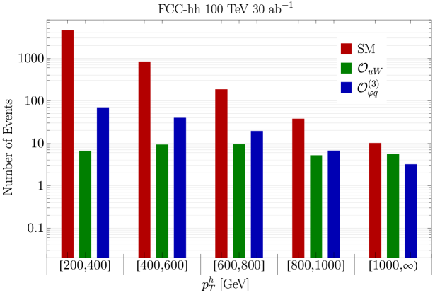
Figure 1: Number of SM and SMEFT events per $p_{T}^{h}$ bin after selection cuts for the signal and backgrounds at the FCC-hh assuming 30 ab^-1. The number of SMEFT events is obtained at the upper bound of the corresponding Wilson coefficients from a single operator fit with 5% syst., i.e. $c_{\varphi q}^{(3)}=3\times 10^{-3}$ and $c_{uW}^{11}=1.1\times 10^{-2}$ with $\Lambda=1$ TeV. Notice that the contribution of ${\cal O}_{\varphi q}^{(3)}$ includes an interference with the SM and could be in principle of either sign. Here we chose the sign such that the interference is positive, i.e. it adds events to the SM prediction.

3.3 Bounds on $\mathcal{O}_{uW}$ from $Wh$ Production

The analysis outlined in the previous subsection allows us to estimate the FCC-hh sensitivity to dipole operators. We show in Tab. 3 the projected bounds on the up-quark EW dipole WC, $c_{uW}$, at FCC-hh with $30$ ab^-1 of integrated luminosity. The first two rows show the bound in the diagonal flavor-aligned scenario, in which $c_{uW}^{11}$ and $c_{uW}^{22}$ are independent WCs. In the third row, we show the result for a light-flavor-universal scenario in which $c_{uW}^{11}=c_{uW}^{22}=c_{uW}$. We do not specify the top-quark WCs, which are associated with negligible effects due to the very small top content of the proton. In our scenario, it would be best constrained by flavor data (see footnote 9). The last row shows the bounds from this analysis on the flavor-universal $c_{\varphi q}^{(3)}$, the WC that this process is most sensitive to. The right column shows the bound from a one-operator fit, while the middle column shows the result of profiling over the other WCs in the fit. For the first two rows, this means profiling over $c_{\varphi q}^{(3)}$ and the other dipole WC, while for the flavor-universal case, it is profiling over $c_{\varphi q}^{(3)}$. Notice that in the IHMFV scenario, the dipole coefficients are related as $c_{uW}^{11}/c_{uW}^{22}=m_{c}/m_{u}\approx 797$, and hence the corresponding bounds would be approximately equal to the ones on $c_{uW}^{11}$.

The projected bounds on $c_{uW}^{11}$ are almost a factor of $4$ worse than the bounds on $c_{\varphi q}^{(3)}$. This was expected from the lack of interference between the dipole operator amplitude and the SM one, and since only one quark flavor, instead of four, contributes to the $c_{uW}^{11}$ bound. The sensitivity to $c_{uW}^{22}$ is a further factor of $\sim 3$ worse due to the lower content of second-generation quarks of the proton. Hence, the flavor-universal results are almost identical to the ones for $c_{uW}^{11}$. The hierarchy in the bounds between $c_{\varphi q}^{(3)}$ and $c_{uW}$ ensures that profiling has a limited impact on the $c_{\varphi q}^{(3)}$ bounds. We checked that using the second binning in $\phi_{W}$ also reduces such impact. For a detailed analysis of the sensitivity to $c_{\varphi q}^{(3)}$, see Ref. Bishara:2020vix .

Coefficient	Profiled Fit	One Operator Fit
$c_{uW}^{11}$	$[-1.33,\,1.33]\times 10^{-2}$ $1\%$ syst. $[-1.39,\,1.39]\times 10^{-2}$ $5\%$ syst. $[-1.47,\,1.47]\times 10^{-2}$ $10\%$ syst.	$[-1.11,\,1.11]\times 10^{-2}$ $1\%$ syst. $[-1.12,\,1.12]\times 10^{-2}$ $5\%$ syst. $[-1.15,\,1.15]\times 10^{-2}$ $10\%$ syst.
$c_{uW}^{22}$	$[-4.2,\,4.2]\times 10^{-2}$ $1\%$ syst. $[-4.5,\,4.5]\times 10^{-2}$ $5\%$ syst. $[-4.7,\,4.7]\times 10^{-2}$ $10\%$ syst.	$[-3.2,\,3.2]\times 10^{-2}$ $1\%$ syst. $[-3.3,\,3.3]\times 10^{-2}$ $5\%$ syst. $[-3.4,\,3.4]\times 10^{-2}$ $10\%$ syst.
$c_{uW}$	$[-1.27,\,1.27]\times 10^{-2}$ $1\%$ syst. $[-1.34,\,1.34]\times 10^{-2}$ $5\%$ syst. $[-1.40,\,1.40]\times 10^{-2}$ $10\%$ syst.	$[-1.05,\,1.05]\times 10^{-2}$ $1\%$ syst. $[-1.07,\,1.07]\times 10^{-2}$ $5\%$ syst. $[-1.09,\,1.09]\times 10^{-2}$ $10\%$ syst.
$c_{\varphi q}^{(3)}$	$[-4.6,\,2.5]\times 10^{-3}$ $1\%$ syst. $[-6.3,\,3.0]\times 10^{-3}$ $5\%$ syst. $[-8.3,\,3.5]\times 10^{-3}$ $10\%$ syst.	$[-2.7,\,2.5]\times 10^{-3}$ $1\%$ syst. $[-3.3,\,2.9]\times 10^{-3}$ $5\%$ syst. $[-4.0,\,3.5]\times 10^{-3}$ $10\%$ syst.

Table 3: Bounds at $95\%$ C.L. on the coefficients of the $c_{uW}^{11}$, $c_{uW}^{22}$, $c_{uW}$(flavor-universal case with $c_{uW}^{11}=c_{uW}^{22}$), and $c_{\varphi,q}^{(3)}$ setting $\Lambda=1\,\text{TeV}$. Left column: bounds profiling over the other coefficients. Right column: bounds with a one operator fit, i.e. setting the other two coefficients to zero. For the flavor-universal case, the bounds of $c_{uW}$ is obtained by profiling over $c_{\varphi q}^{(3)}$ or set it to zero. The profiled bound on $c_{\varphi q}^{(3)}$ was obtained in the case of free $c_{uW}^{11}$ and $c_{uW}^{22}$.

In Fig. 2, we show the $95\%$ C.L. on the planes $c_{\varphi q}^{(3)}-c_{uW}^{11}$ (left panel) and $c_{\varphi q}^{(3)}-c_{uW}^{22}$ (right panel). In both cases, we show the result of profiling over the other dipole WC (full line), setting it to zero (dashed line) or linking it via flavor universality (dotted line). In the latter case, the x-axis should be read as $c_{uW}$. The left panel shows that setting $c_{uW}^{22}=0$ or $c_{uW}^{22}=c_{uW}^{11}$ has a negligible impact since our analysis is mostly sensitive to the first-generation quarks. However, profiling over $c_{uW}^{22}$ explores larger values of $c_{uW}^{22}$ and causes a sizeable difference in the correlation between $c_{\varphi q}^{(3)}$ and $c_{uW}^{11}$ for negative values of the former. The opposite situation can be observed in the right panel, where each choice for $c_{uW}^{11}$ causes very different results, especially for negative $c_{\varphi q}^{(3)}$. In particular, setting $c_{uW}^{11}=c_{uW}^{22}$ generates much tighter bounds.

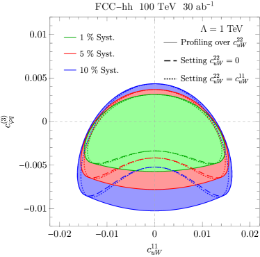
Figure 2: Expected $95\%$ C.L. bounds on $c_{uW}^{11}$, $c_{uW}^{22}$, $c_{\varphi q}^{(3)}$ at the FCC-hh for $30\,\text{ab}^{-1}$.

Had we considered the $h\to b\bar{b}$ decay channel and adopted the analysis from Ref. Bishara:2022vsc , the projected bounds at FCC-hh would have been of the same order of magnitude, in particular for $5\%$ syst. uncertainty. The projections in Ref. Bishara:2022vsc degrade by a factor of $\sim 5-6$ when going from FCC-hh to HL-LHC. Hence, we estimate that their analysis for the 1-lepton channel, i.e. $Wh$, could yield the bounds $|c_{uW}^{11}|\lesssim 6\times 10^{-2}$, $|c_{uW}^{22}|\lesssim 2\times 10^{-1}$, and $|c_{uW}|\lesssim 6\times 10^{-2}$ with $\Lambda=1$ TeV. This should be compared against current and projected bounds from other collider processes. For instance, the quark dipole operator has also been studied with Drell-Yan data from LHC daSilvaAlmeida:2019cbr ; Boughezal:2021tih ; Allwicher:2022gkm . For $\Lambda=1$ TeV, Ref. daSilvaAlmeida:2019cbr obtain $|c_{uW}|<3.8\times 10^{-1}$ from a single-operator fit and $|c_{uW}|<5.3\times 10^{-1}$ from a profiled fit, in agreement with Ref. Boughezal:2021tih . Assuming that these bounds are statistically limited, we can rescale them to HL-LHC luminosity and obtain $|c_{uW}|\lesssim 1\times 10^{-1}$ and $|c_{uW}|\lesssim 2\times 10^{-1}$, which is similar or worse than our estimates from $Wh$ production. Ref. Allwicher:2022gkm finds slightly better bounds from LHC data, $|c_{uW}^{11}|\lesssim 1.4\times 10^{-1}$ and $|c_{uW}^{22}|\lesssim 5.7\times 10^{-1}$, which could become equal to our $Wh$ estimates at HL-LHC. In addition to high-energy tails, electroweak precision data also constrains the light quark dipole coupling to electroweak gauge bosons; for instance the coefficient $c_{uW}$ will modify the $Z$ decay width. However, these bounds are weak, $|c_{uW}|\lesssim 10$, in part due to the mass-suppressed interference between the SM and dipole amplitudes Escribano:1993xr ; Kopp:1994qv ; daSilvaAlmeida:2019cbr ; Brivio:2019myy . Therefore, the high-energy regime of $Wh$ could be a useful probe of light-quark EW dipole operators at HL-LHC and FCC-hh.

Finally, it is instructive to assess the EFT validity in this analysis. In agreement with what was found in Ref. Bishara:2020vix , the bounds presented before are valid for an EFT cutoff $\gtrsim 5$ TeV, while they degrade slightly for a cutoff $\sim 2-5$ TeV and the analysis becomes invalid for lower cutoff scales. To properly interpret our bounds in terms of UV physics, it is also worth mentioning that the dipole operators are only generated at the 1-loop level in weakly coupled theories Craig:2019wmo , so that one might expect a naive bound of $c_{uW}\sim\frac{\mathcal{O}(1)}{16\pi^{2}}\approx 6.3\cdot 10^{-3}$ which is beyond the reach of most of our bounds. However, we expect a scaling $c_{uW}\sim\frac{g\,g_{*}^{3}}{16\pi^{2}M^{2}}$, where $g_{*}$ is the coupling between UV and SM fields, for a typical UV model. Our bounds would then mean that we are probing $g_{*}\gtrsim 3.9$. Such couplings, despite being large, remain well within the perturbative regime $g_{*}<\,4\pi$ Giudice:2007fh ; Manohar:1983md ; Georgi:1986kr .

Another marker of a possible EFT validity loss would be a relevant contribution from operators of dimension 8 or higher. Indeed, due to the lack of interference between the SM and dipole amplitudes, dimension-8 operators contribute at the same order, $\Lambda^{-4}$, in the SMEFT expansion. Motivated by the fact that recent studies in the geoSMEFT framework indicate that contributions to $Wh$ production from interference between dimension-8 and SM amplitudes are highly suppressed by the SM couplings Corbett:2023yhk , and by the fact that we would also need to make flavor and operator assumptions at dimension-8, themselves backed by UV model examples as in Sec. 5, we neglect dimension-8 contributions. Nevertheless, a more precise study of their impact on dipole bounds using any of the SMEFT dimension-8 bases would be interesting and is left for future work.

4 Low Energy Constraints

In this section, we explore the constraints that are imposed by low-energy data on EW quark dipoles in flavor-aligned scenarios. Usually, bounds on contributions to flavor-changing currents beyond the SM involving the first two generations give stringent constraints on off-diagonal flavorful couplings, pushing the NP scale to high values. However, we will show that those constraints loosen significantly in the case of the EW up-quark dipole $\mathcal{O}_{uW}$ in the flavor-aligned scenario when new spurions only appear in the up sector. We will also analyze the particular case of IHMFV. Overall, the flavor bounds turn out to be much weaker than the collider ones.

We remind the reader that, as explained above, we needed to assume the absence of any new CP-odd spurion beyond that of the SM, due to the strong EDM constraints on the imaginary part of dipole operators. Also, if additional SMEFT operators are present, we need to assume that those most restricted by low-energy flavor data, such as purely left-handed 4-Fermi operators, do not communicate with the new flavor-breaking spurions. We also remind that we illustrate how the above assumptions are realized in a UV model in Sec. 5.

In the SM and beyond, translating low-energy flavor bounds to the level of UV models first requires that one integrates weak-scale dynamics out, matching it to the Weak Effective Theory (WET) Hamiltonian Jenkins:2017jig ; Jenkins:2017dyc ; Dekens:2019ept ,

$$\mathcal{H}_{\rm eff}=G_{F}\sum_{i}C_{i}\mathcal{Q}_{i}+{\rm h.c.}\;,$$ (13)

where $G_{F}$ is the Fermi constant and $C_{i}$ are Wilson coefficients. The latter run to lower energies until the QCD scale, where a theory of hadrons, most particularly Chiral Perturbation Theory ($\chi$PT) for the light mesons, takes over. Through this matching and running procedure Buchalla:1995vs ; Aebischer:2015fzz ; Celis:2017hod ; Jenkins:2017jig ; Jenkins:2017dyc ; Aebischer:2018bkb ; Hurth:2019ula ; Dekens:2019ept , one can obtain constraints on the WET WCs and on NP from those on FCNC, arising from various meson experiments. In particular, rare kaon decays are sensitive low-energy probes of BSM physics Cirigliano:2011ny .

Under our flavor assumption that only the dipole has a non-MFV flavor structure in the SMEFT, tree-level processes are either MFV-suppressed or flavor-changing charged currents (FCCC), while FCNC will arise at the loop level. We discuss both types of processes in the following sections. We finally explore the constraints imposed by the naturalness of the quark masses at the weak scale.

4.1 FCNC

The most stringent flavor bounds usually arise from FCNC, hence we start our analysis from those. Even when they are absent at tree level, some of the FCNC operators in (13) are generated at loop level by the dipole, as shown in Fig. 3. This figure shows diagrams with $\Delta F=1$ (where $\Delta F=\Delta S,\,\Delta C$) and two insertions of the dipole operator that generate FCNC in the down-quark sector. Diagrams with a single insertion are suppressed by the GIM mechanism, hence they are up-Yukawa-suppressed, and we have checked that they are smaller in magnitude for cutoffs close to the collider bounds. For IHMFV, they are either down-Yukawa-suppressed or flavor-diagonal. Diagrams in the up sector are flavor-diagonal or strongly suppressed by the down Yukawa. Finally, $\Delta F=2$ operators are suppressed by the GIM mechanism and by MFV in the down sector.

Figure 3: Feynman diagrams with two up-dipole insertions (represented by the large black dots) inducing $\Delta S=1$ WET operators. In the first row, fermion lines on the right side of the diagrams can be either leptons $\ell$ or quarks $q$. In the second row, the external gauge boson in the first diagram could also be a gluon.

Therefore, in this subsection, we focus on WET operators generated by diagrams featuring two dipole insertions and giving rise to $\Delta S=1$ processes (Those are the most sensitive $\Delta F=1$ processes given our flavor assumption.). They are the following,

$$\begin{aligned} &\mathcal{Q}_{\ell 1}=(\bar{d}\gamma^{\mu}P_{L}d)(\bar{\ell}\gamma_{\mu}P_{L}\ell)\;,\quad\mathcal{Q}_{7\gamma}^{(\prime)}=em_{d_{R}}\left(\bar{d}\sigma^{\mu\nu}P_{R(L)}d\right)F_{\mu\nu}\;,\\ &\mathcal{Q}_{q3}=\left(\bar{d}\gamma^{\mu}P_{L}d\right)\left(\bar{q}\gamma_{\mu}P_{L}q\right)\;,\quad\mathcal{Q}_{8g}^{(\prime)}=g_{s}m_{d_{R}}\left(\bar{d}\sigma^{\mu\nu}P_{R(L)}T^{A}d\right)G^{A}_{\mu\nu}\;,\end{aligned}$$ (14)

where $q$ represents any type of quark, $\ell$ is any kind of lepton, and the generation indices are kept implicit. We explicitly pulled a quark mass out of the Wilson coefficients of the magnetic and chromo-magnetic dipoles, since it arises from the diagram in Fig. 3, due to our assumption on the flavor and operator structure in the SMEFT.

They contribute to several flavor-changing processes involving mesons, and we consider here kaon decays to lepton pairs or photon pairs, as well as $K^{+}\rightarrow\pi^{+}\pi^{0}\gamma$. $K\rightarrow\pi\pi$ can also be induced by $\mathcal{Q}_{q3}$ and $\mathcal{Q}_{8g}^{(\prime)}$ Pich:2021yll , however, current uncertainties in SM computations via lattice simulations limit the accuracy in determining chiral Lagrangian parameters. Therefore, we leave a discussion of $K\rightarrow\pi\pi$ to App. B.1. For a given process, several operators in Eq. (LABEL:eq:WETops) are likely to contribute at a given order in $\chi$PT. For instance, both the photon and gluon dipoles can contribute to $K\rightarrow\gamma\gamma$ at ${\cal O}(p^{6})$, or the 4-quark operator $\mathcal{Q}_{q3}$ can contribute to $K^{+}\rightarrow\pi^{+}\pi^{0}\gamma$ through the inner bremsstrahlung good1959pion . We leave a precise determination of each operator contribution for future work, and focus on that of $\mathcal{Q}_{\ell 1}$ and $\mathcal{Q}_{7\gamma}^{(\prime)}$. We checked that all other contributions to the processes of interest are smaller or equal according to the $\chi$PT power counting, so $\mathcal{Q}_{\ell 1}$ and $\mathcal{Q}_{7\gamma}^{(\prime)}$ serve as a proxy for the full result. As we will show, the resulting bounds are weaker than collider ones, which justifies a posteriori that an order-of-magnitude analysis is sufficient.

The Wilson coefficients of $\mathcal{Q}_{\ell 1}$ and $\mathcal{Q}_{7\gamma}^{(\prime)}$ are the following,

$$C_{\ell 1}=\frac{z_{\ell 1}c_{uW}c_{uW}^{\dagger}m_{W}^{2}}{16\pi^{2}G_{F}\Lambda^{4}}\;,\quad C_{7\gamma}=C_{7\gamma}^{\prime}=\frac{z_{7\gamma}c_{uW}c_{uW}^{\dagger}v_{h}^{2}}{16\pi^{2}G_{F}\Lambda^{4}}\;,$$ (15)

where the values of $z_{i}$ are log-dependent of the renormalization scale $\mu\sim m_{K}$. We find that the leading contribution of $z_{i}$ are about $\mathcal{O}(10)$, $z_{\ell 1}\approx 3\log(m_{W}/m_{K})+3/2$, and $z_{7\gamma}\approx(10/9)\log(m_{W}/m_{K})-277/54$. Using our flavor assumption from Eq. (5), if $c_{uW}^{11}$ is not accidentally small, the off-diagonal components of the Wilson coefficients depend on $\left(c_{uW}c_{uW}^{\dagger}\right)_{i\neq j}\approx\left|c_{uW}^{11}\right|^{2}\tilde{\lambda}_{\rm FC}$, which is real at the leading order, so that we can focus on FCNC constraints applicable to the real components of $C_{i}$. (We nonetheless remind that we have assumed no new source of CP violation.)

The experimental bounds on $C_{\ell 1}$ can be obtained from kaon leptonic decays. They also receive a contribution from $C_{7\gamma}^{(\prime)}$, but it is suppressed by $\sin^{2}\theta_{\rm w}m_{s}/m_{K}$. The most stringent limits on BSM physics arise from $K_{L}\rightarrow\ell^{+}\ell^{-}$, for which the SM prediction has been recently improved Hoferichter:2023wiy . Normalizing to the $K_{L}\rightarrow\gamma\gamma$ decay, the decay rate can be expressed in terms of the reduced amplitude $\mathcal{A}_{\ell}$ Cirigliano:2011ny ,

$$R_{L}^{\ell}=\frac{{\rm BR}(K_{L}\rightarrow\ell^{+}\ell^{-})}{{\rm BR}(K_{L}\rightarrow\gamma\gamma)}=2\sqrt{1-\frac{4m_{\ell}^{2}}{m_{K}^{2}}}\left(\frac{\alpha_{\rm em}m_{\ell}}{\pi m_{K}}\right)^{2}\left|\mathcal{A}_{\ell}\right|^{2}\;.$$ (16)

Using ${\rm BR}(K_{L}\rightarrow\gamma\gamma)=5.47(4)\times 10^{-4}$ Workman:2022ynf , the experimental value of $R_{L}^{\mu}$ implies that ${\rm Re}\,\mathcal{A}_{\mu}^{\rm exp}=\pm 1.16(24)$, while the SM prediction is ${\rm Re}\,\mathcal{A}_{\mu}^{\rm SM}=-1.96(36)$ Hoferichter:2023wiy . Assuming the negative value for ${\rm Re}\,\mathcal{A}_{\mu}^{\rm exp}$, we can derive the BSM constraint ${\rm Re}\,\mathcal{A}_{\mu}^{\rm BSM}=0.80(43)$. The presence of $\mathcal{Q}_{\ell 1}$ leads to

$${\rm Re}\,\mathcal{A}_{\ell}^{\rm BSM}=\frac{\pi G_{F}m_{K}f_{K}C_{\ell 1}^{ds}}{\alpha_{\rm em}}\sqrt{\frac{m_{K}}{16\pi\Gamma(K_{L}\rightarrow\gamma\gamma)}}\;,$$ (17)

where $f_{K}=35\,\text{MeV}/V_{us}$ Workman:2022ynf refers to the meson decay constant. Demanding that the contribution of the WET operator ${\cal Q}_{\ell 1}$ does not exceed the discrepancy encoded in $\mathcal{A}_{\mu}^{\rm BSM}$, we obtain a $95\%$ C.L. bound on $C_{\ell 1}^{ds}$ of $[-0.1,3.6]\times 10^{-6}$, which translates into a $95\%$ C.L. upper bound on $c_{uW}^{11}$,

$$|c_{uW}^{11}|<0.5\left(\Lambda/\text{TeV}\right)^{2}\;.$$ (18)

This bound, the strongest of the ones that we derive in this section, is weaker than the projected collider bounds presented in Tab. 3 and, in particular, at best of the same order than our estimates for HL-LHC. Turning now to the dipole operator $\mathcal{Q}_{7\gamma}^{(\prime)}$, it can induce $d_{i}\rightarrow d_{j}\gamma$ transition. The magnetic and electric dipole WET operators are commonly defined in the basis Mertens:2011ts as follows,

$$Q_{\gamma}^{\pm}=\frac{Q_{d}e}{16\pi^{2}}(\bar{s}_{L}\sigma^{\mu\nu}d_{R}\pm\bar{s}_{R}\sigma^{\mu\nu}d_{L})F_{\mu\nu}\;,$$ (19)

where we can relate $C_{7\gamma}^{(\prime)}$ to the Wilson coefficients of the new operators via

$$C_{7\gamma}^{21}=\frac{Q_{d}\left(C_{\gamma}^{+}+C_{\gamma}^{-}\right)}{16\pi^{2}G_{F}m_{d}}\;,\quad C_{7\gamma}^{\prime 21}=\frac{Q_{d}\left(C_{\gamma}^{+}-C_{\gamma}^{-}\right)}{16\pi^{2}G_{F}m_{s}}\;.$$ (20)

In the SM, the estimated value of the real component of $C_{\gamma}^{\pm}$, denoted as $\left|{\rm Re}\,C_{\gamma}^{\pm}\right|^{\rm SM}$, is approximately $0.06\,G_{F}\,m_{K}$, and the experimental constraints on $C_{\gamma}^{\pm}$ are derived from the processes $K^{+}\rightarrow\pi^{+}\pi^{0}\gamma$ and $K^{0}\rightarrow\gamma\gamma$ Mertens:2011ts . The $s\rightarrow d\gamma$ contributions consist of an electric ($\propto C_{\gamma}^{-}$) and magnetic component $(\propto C_{\gamma}^{+})$. Among them, the electric amplitude is more precisely measured and leads to the constraint, $|{\rm Re}\,C_{\gamma}^{-}|<0.1\,G_{F}\,m_{K}$.

For $K_{S}\rightarrow\gamma(k_{1},\mu)\gamma(k_{2},\nu)$ decay amplitudes, the photons produced in this decay have parallel polarization, $\mathcal{A}(K^{0}\rightarrow(\gamma\gamma)_{\parallel})\times\left(k_{1}^{\nu}k_{2}^{\mu}-k_{1}\cdot k_{2}g^{\mu\nu}\right)$, while the photon produced by $K_{L}\rightarrow\gamma\gamma$ have perpendicular polarization, $\mathcal{A}(K^{0}\rightarrow(\gamma\gamma)_{\perp})\times i\varepsilon_{\mu\nu\rho\sigma}k_{1}^{\rho}k_{2}^{\sigma}$ . In this notation, the decay width is given by $\Gamma(K^{0}\rightarrow\gamma\gamma)=m_{K}^{3}|\mathcal{A}|^{2}/64\pi$. Parametrizing the amplitudes as Mertens:2011ts ,

$$\begin{aligned} \mathcal{A}(K^{0}\rightarrow(\gamma\gamma)_{\parallel})=\frac{A_{\gamma\gamma}^{\parallel}}{\sqrt{2}}\times(\alpha_{\rm em}G_{F}m_{K})\;,\quad\mathcal{A}(K^{0}\rightarrow(\gamma\gamma)_{\perp})=\frac{A_{\gamma\gamma}^{\perp}}{\sqrt{2}}\times(\alpha_{\rm em}G_{F}m_{K})\;,\end{aligned}$$ (21)

we can fix $|A_{\gamma\gamma}^{\parallel}|^{\rm exp}=0.191$ and $|A_{\gamma\gamma}^{\perp}|^{\rm exp}=0.115$ from the $K_{L,S}\rightarrow\gamma\gamma$ decay rates Workman:2022ynf . The dipole operator $Q_{\gamma}^{\pm}$ contribute to the kaon diphoton decay amplitude Mertens:2011ts as

$$\Delta A_{\gamma\gamma}^{\parallel,\perp}=\frac{2F_{\pi}B_{T}^{\prime}C_{\gamma}^{-,+}}{9\pi G_{F}m_{K}^{2}}\;,$$ (22)

where $F_{\pi}=92.4\,\text{MeV}$ and $B_{T}^{\prime}=2.67(17)$ is extracted from the lattice estimation Buividovich:2009bh . The SM prediction, $|A_{\gamma\gamma}^{\parallel}|^{\rm SM}=0.166$ and $|A_{\gamma\gamma}^{\perp}|^{\rm SM}=0.126$ provides constraints $|{\rm Re}\,C_{\gamma}^{-}|<0.7\,G_{F}\,m_{K}$, and $|{\rm Re}\,C_{\gamma}^{+}|<0.3\,G_{F}\,m_{K}$. This turns into the following bound

$$|c_{uW}^{11}|<40.3\left(\Lambda/\text{TeV}\right)^{2}\;.$$ (23)

from the $K^{0}\rightarrow\gamma\gamma$ channel.

4.2 FCCC

Beyond the aforementioned loop-level FCNC, our flavor assumptions lead to tree-level FCCC. Some of those, including the pion decay $\pi^{-}\rightarrow e^{-}\bar{\nu}_{e}\gamma$ on which we focus below, can be worked out by treating the $W$ boson field strength in the EW dipole of Eq. (1) as an external source that extends the QCD Lagrangian, and that ought to be integrated out afterwards in $\chi$PT. In particular, the effect of other tree-level operators such as 4-quark operators is subleading.

The decay $\pi^{-}\rightarrow e^{-}\bar{\nu}_{e}\gamma$ decay requires an operator with a $W$ boson and a photon. Combining the $W$ boson field strength and the SMEFT WC $c_{uW}$ in Eq. (1) into a chiral tensor spurion $t_{\mu\nu}$, we follow Refs. Cata:2007ns ; Mateu:2007tr and match to the lowest-order operator involving a photon field strength in $\chi$PT,

$$\mathcal{L}^{\chi{\rm PT}}\supset\frac{B_{0}F_{\pi}^{2}}{M_{\rho}^{2}}\text{Tr}\left(t_{+}^{\mu\nu}f_{+\mu\nu}\right)\;,$$ (24)

where $B_{0}F_{\pi}^{2}=-\langle\bar{q}q\rangle=-[242(15)\,{\rm MeV}]^{3}$ Jamin:2002ev , $M_{\rho}=0.775\,\text{GeV}$ is the $\rho$ meson mass, and the definitions of $t_{+}^{\mu\nu}$ and $f_{+\mu\nu}$ are given in App. B.2. Expanding to leading order in $F_{\pi}$ one finds,

$$\begin{aligned} \mathcal{L}^{\chi{\rm PT}}_{1}\supset\frac{i2\,e\,B_{0}\,F_{\pi}G_{F}v_{h}V_{ud}\,c_{uW}^{11}}{3g_{2}M_{\rho}^{2}\Lambda^{2}}\partial_{\mu}\pi^{+}J_{\nu}^{-}\left(F^{\mu\nu}+i\tilde{F}^{\mu\nu}\right)+{\rm h.c.}\;,\end{aligned}$$ (25)

where $J_{\mu}^{-}=\bar{\nu}\gamma^{\mu}P_{L}e$ is the weak current and $\tilde{F}_{\mu\nu}=\epsilon_{\mu\nu\rho\sigma}\,F^{\rho\sigma}/2$. This implies that the quark dipole can induce additional contributions to the form factors $F_{V}$ and $F_{A}$ describing the $\pi^{-}\rightarrow e^{-}\bar{\nu}_{e}\gamma$ decay amplitude $\mathcal{M}_{\rm SD}$ Belyaev:1991gs ; Bolotov:1990yq ,

$$\mathcal{M}_{\rm SD}=-\frac{e\,G_{\rm F}V_{ud}}{\sqrt{2}m_{\pi}}\epsilon^{*\mu}\left[F_{V}\epsilon_{\mu\nu\sigma\tau}\,p^{\sigma}q^{\tau}+iF_{A}(g_{\mu\nu}\,p\cdot q-p_{\nu}q_{\mu})\right]\bar{u}\gamma^{\nu}(1+\gamma^{5})v\ .$$ (26)

From Eq. (25) and  (26), we get,

$$\Delta F_{V}=\Delta F_{A}=\frac{4\sqrt{2}\,c_{uW}^{11}\,B_{0}F_{\pi}v_{h}m_{\pi}}{3\,g_{2}\,M_{\rho}^{2}\Lambda^{2}}\;.$$ (27)

The theoretical values of the pion form factor is related to the conserved vector current to the $\pi^{0}\rightarrow\gamma\gamma$ decay width muller1963connection ; Unterdorfer:2008zz ,

$$\begin{aligned} F_{V}^{\rm SM}&=\alpha_{\rm em}^{-1}\sqrt{2\,\Gamma_{\pi^{0}\rightarrow\gamma\gamma}/(\pi m_{\pi^{0}})}=0.0262(5)\\ F_{A}^{\rm SM}&=4\sqrt{2}\left(L_{9}+L_{10}\right)m_{\pi^{+}}/F_{\pi}=0.0106(36)\ .\end{aligned}$$ (28)

In this context, $L_{9}$ and $L_{10}$ are the coefficients within the general $\chi$PT of order $\mathcal{O}(p^{4})$ as outlined in Gasser:1984gg . Their phenomenological vaules are detailed in Bijnens:1992en . The experimental values of the form factors are measured by the CsI crystal calorimeter of PIBETA group Bychkov:2008ws , $F_{V}^{\rm exp}=0.0258(17)$, $F_{A}^{\rm exp}=0.0117(17)$. Assuming that the dipole contribution to $F_{V,A}$ can not exceed the discrepancy between the SM prediction and the measured value we can bound the dipole WC as,

$$|c_{uW}^{11}|<13\left(\Lambda/\text{TeV}\right)^{2}\;.$$ (29)

4.3 Quark Mass Naturalness

Finally, we investigate naturalness constraints on the quark masses. As we are introducing additional spurions beyond the quark Yukawas with sizable entries along the light generations, radiative contributions to the low-energy quark masses potentially lead to an up-quark hierarchy problem.

The one-loop diagram that renormalizes the up-quark mass with one dipole insertion gives,

$$\begin{aligned} \frac{\delta m_{u}}{m_{u}}=\frac{3c_{uW}^{11}m_{W}}{2m_{u}\Lambda^{2}}\int_{0}^{E}\frac{d^{4}q}{(2\pi)^{4}}\frac{q_{\mu}\sigma^{\mu\nu}\not{q}\gamma_{\nu}}{q^{2}(q^{2}-m_{W}^{2})}\sim\frac{3c_{uW}^{11}m_{W}E^{2}}{16\pi^{2}m_{u}\Lambda^{2}}\;,\end{aligned}$$ (30)

where we considered a hard cutoff $E$ to extract the quadratic divergence, which we take as a proxy for possible threshold corrections at scales $\sim\Lambda$. If we require one percent tuning, $|\delta m_{u}/m_{u}|<100$, the quark Yukawa naturalness provides an upper bound on the Wilson coefficient,

$$|c_{uW}^{11}|\lesssim 0.1\;.$$ (31)

In appropriate UV models, threshold corrections to the small up-quark mass can be controlled employing symmetry. For instance, Ref. Voloshin:1987qy argues that a suppressed neutrino mass accompanied by a sizeable magnetic dipole could result from an $SU(4)$ symmetry in the lepton sector. A similar symmetry in the quark sector could suppress the light-quark Yukawa couplings, but we leave the development of a precise model for future work.

5 A Renormalizable UV Model

In this section, we explore fully renormalizable theories that can give rise to $c_{uW}$ as in Eq. (7), and to no other dangerous flavorful SMEFT operators. As IHMFV is a subclass of alignment as we defined it, we take this model as proof of principle that either of them can be obtained from weakly-coupled UV completions.

To this end, we introduce a set of heavy vector-like fermions $F$, $X$ and a complex scalar $S$. The fermions come in three generations, and the SM charges of the new fields are listed in Tab. 4.

BSM Fields	$F$	$S$	$X$
$G_{\rm SM}$	$(\mathbf{3},\mathbf{2},\frac{1}{6})$	$(\mathbf{1},\mathbf{1},0)$	$(\mathbf{3},\mathbf{2},\frac{1}{6})$

Table 4: Standard Model gauge charges of the heavy BSM fields of our renormalizable UV model.

As we are aiming at deriving IHMFV, we need to specify the (spurious) flavor transformations of all building blocks (fields and couplings) of the theory. IHMFV arising from regular MFV in the UV, we assume that the flavor non-universal interactions depend on a single spurion $Y_{u}$. Focusing on the active subset $G_{F}^{q}\equiv SU(3)_{Q}\times SU(3)_{u}$ of the flavor group, we assume the transformations in Tab. 5.

Names	$Q_{L}$	$u_{R}$	$\mathbb{P}_{L}F$	$\mathbb{P}_{R}F$	$\mathbb{P}_{L}X$	$\mathbb{P}_{R}X$	$S$	$Y_{u}$
$G_{F}^{q}$	$(\mathbf{3},\mathbf{1})$	$(\mathbf{1},\mathbf{3})$	$(\mathbf{3},\mathbf{1})$		$(\mathbf{1},\mathbf{3})$	$(\mathbf{3},\mathbf{1})$	$(\mathbf{1},\mathbf{1})$	$(\mathbf{3},\mathbf{\bar{3}})$
$U(1)_{M}$	$0$		$q$		$-q$		$0$

Table 5: Global symmetry charges of the relevant fields in our renormalizable UV model. Among them $Y_{u}$ functions as a spurion, whereas the remaining fields are dynamical.

We also indicate there the charges under a global unbroken $U(1)_{M}$ symmetry. No new field is introduced in the down sector, and $Y_{d}$ is the only spurion with down-type charges. The most general Lagrangian respecting all (spurious) symmetries reads

$$\begin{aligned} \mathcal{L}=&\bar{Q}_{L}\lambda_{q}FS+\bar{F}\lambda_{F}\mathbb{P}_{R}S^{\dagger}X+\bar{X}\lambda_{u}u_{R}\widetilde{H}+\bar{X}MY_{u}^{\dagger}\mathbb{P}_{R}X+\bar{Q}_{L}mX\\ &+\bar{X}\xi Y_{u}^{\dagger}\mathbb{P}_{R}FS+\bar{Q}_{L}Y_{u}u_{R}\widetilde{H}+\bar{F}M_{F}\mathbb{P}_{R}F+{\rm h.c.}+m_{S}^{2}|S|^{2}\ .\end{aligned}$$ (32)

$m$ mixes $Q_{L}$ with X, but this mixing can be removed by a field redefinition. Therefore, in what follows we consider $m=0$. Most masses and Yukawa couplings above transform in a singlet or adjoint representation of the flavor group: $\lambda_{q},\lambda_{F},m,M_{F}$ transform as $(\mathbf{1}\oplus\mathbf{8},\mathbf{1})$, while $\lambda_{u},M,\xi$ transform as $(\mathbf{1},\mathbf{1}\oplus\mathbf{8})$. Therefore, they admit an expansion in terms of the only flavorful building blocks, $Y_{u,d}$. Assuming only positive powers of those spurions, we have

$$\lambda_{q}\propto\mathbb{1}+a_{1}X_{u}+a_{2}X_{d}+\cdots\;,\quad\lambda_{u}\sim\mathbb{1}+b_{2}Y_{u}^{\dagger}Y_{u}+\cdots\;,$$ (33)

where $X_{u,d}\equiv Y_{u,d}^{\phantom{\dagger}}Y_{u,d}^{\dagger}$, as defined in Sec. 2. This expansion leads to flavor-changing matrix elements suppressed by the normal MFV mechanism. We stress that renormalization group running will slightly misalign the flavor structures of the various couplings, so that they will not be captured by a single spurion $Y_{u}$ at all scales. Therefore, the Lagrangian in Eq. (32) is meant to hold at a high scale, for instance that of spontaneous breaking of the flavor group where the Yukawas are generated, if such a mechanism occurs. Nevertheless, the hierarchies inherited at the high scale, which are the main focus of this work, will not be drastically affected by that running.

Integrating out the BSM fields $F$, $S$ and $X$ at one loop we get,

$$\frac{c_{uW}}{\Lambda^{2}}=\frac{g_{2}\lambda_{q}\lambda_{F}M_{F}\hat{M}_{X}^{-1}\lambda_{u}}{128\pi^{2}m_{S}^{2}}\mathcal{F}_{2}^{C}(r)\ ,$$ (34)

where $\hat{M}_{X}\equiv Y_{u}^{\dagger}M$ is the mass matrix of $X$ and the loop function $\mathcal{F}_{2}^{C}$ is given by

$$\mathcal{F}_{2}^{C}\left(r\right)=\frac{3}{2}\frac{[3-4r+r^{2}+2\ln(r)]}{(r-1)^{3}},\quad\text{with }r=\frac{(y_{2}\,M)^{2}}{m_{S}^{2}}\ .$$ (35)

The SMEFT cut-off scale is set by the lightest BSM particles, $\Lambda\sim\text{min}\left(M_{S},M_{F},y_{u}M\right)$. In Eq. (34), $\hat{M}_{X}$ is the only hierarchical matrix in flavor space, so the flavor structure of $c_{uW}$ is dictated by the inverse Yukawa, $c_{uW}\propto\widetilde{Y}_{u}$. This realizes IHMFV. Due to the MFV expansion of $\lambda_{q,u}$, the off-diagonal components of $c_{uW}$ in the up basis is suppressed by $\lambda_{\rm FC}$,

$$c_{uW}^{12}\sim c_{uW}^{11}\lambda_{\rm FC}^{12}\sim\lambda^{5}c_{uW}^{11}\;.$$ (36)

As discussed in Sec. 2.2, in IHMFV large flavor-changing effects can be mediated by other SMEFT operators than the dipole, in particular by the LL-type 4-quark operators. However, those turn out to be flavor-blind in the model presented here. A detailed discussion can be found in App. C, where we show all the dimension-6 SMEFT operators induced by the model in Eq. (32), up to one-loop level.

6 Conclusion and Discussion

SMEFT provides a convenient and consistent description of physics beyond the SM when the new particles are heavy enough to not be produced on-shell at a given experiment. The effects of different UV models are encoded in the Wilson Coefficients that weigh the SMEFT higher-dimensional operators. Given that the vast majority of the free coefficients in the SMEFT is associated with the existence of three generations, i.e. flavor physics, and given that the bounds arising from searches for non-standard flavor violation vastly dominate other ones for random WCs, it is important to deeply investigate the flavor structure of the SMEFT. This has been done in the past from a variety of perspectives, most notably from that of specific UV models and from that of flavor symmetries.

In the realm of flavor symmetries, the most common framework is Minimal Flavor Violation, where one assumes that the only flavor-breaking spurions that one can use to build SMEFT WCs are the SM Yukawa couplings. This strongly alleviates FCNC constraints on the scale of new physics. However the MFV paradigm only represents a subset of the possible EFTs that evade flavor bounds. In this work, we scrutinized a flavor structure in the SMEFT which has been dubbed flavor alignment in previous literature. This structure is similar to MFV in that flavor violation is fully dictated by the SM CKM matrix, while it radically differs in that WCs do not follow the same hierarchies as quark masses and couplings to the Higgs boson. In short, light generations are allowed to couple to large flavor-breaking spurions which are only misaligned from quark masses by the CKM matrix. We also investigated a more restrictive assumption, which we call inverse hierarchy MFV, in which the new aligned spurions are proportional to the inverse of the Yukawa matrices.

As it stands, those assumptions are not as efficient as MFV to weaken FCNC bounds. However, this depends on the set of SMEFT operators under consideration. We focused on the up-type quark electroweak dipole operator $\mathcal{O}_{uW}$, for which we demonstrated that the bounds from flavor violation are rather weak, even for dipoles of the light quark generations. Instead, we showed that those dipoles are much better probed at hadron colliders.

More precisely, this can be done by looking at the high-energy tails in $Wh$ production at hadron colliders. Indeed, the $pp\rightarrow Wh$ process is dominated by the light quark operators allowed by our flavor assumptions. We showed how a simple analysis at FCC-hh could provide competitive bounds when the final state is $\ell\nu\gamma\gamma$. A simple scaling based on comparison with previous analyses showed that the same process, but with the Higgs decaying to $b\bar{b}$, would yield relevant bounds at HL-LHC, even in comparison against projected bounds from Drell-Yann high-energy tails. In Fig. 4, we summarize our projected bounds for FCC-hh and other current or projected bounds. We only show the general flavor scenario since the flavor-universal case gives results very similar to the ones for the first-generation quarks. This plot shows the potential of $Wh$ production as a probe of EW dipoles in the flavor scenario presented in this work.

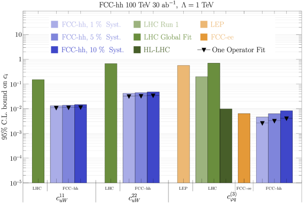
Figure 4: $95\%$ C.L. bounds on $c_{uW}^{11}$, $c_{uW}^{22}$, and $c_{\varphi q}^{(3)}$. We show in blue our bounds from a one-operator fit of $Wh\to\ell\nu\gamma\gamma$ at FCC-hh with 30 ab^-1 for different systematic uncertainties. The filled bars give the bounds after profiling over the other WCs in the analysis, while the horizontal black line with a triangle indicates the bounds from one-operator fits. In green for $c_{uW}^{11}$ and $c_{uW}^{22}$, the bounds are taken from the HighPT fit Allwicher:2022gkm . For $c_{\varphi q}^{(3)}$, the lighter and darker green bounds are from LHC and HL-LHC using leptonic $WZ$ Franceschini:2017xkh , and the bounds in medium green is from a global fit Ellis:2018gqa . In lighter and darker orange for $c_{\varphi q}^{(3)}$, the bounds are from LEP Franceschini:2017xkh and FCC-ee global fit DeBlas:2019qco .

Finally, we presented a UV model that realizes our flavor and operator assumptions. Its UV flavor structure follows the regular MFV assumption, and it features heavy massive fields that transform chirally under the flavor group, so that the induced low-energy EFT follows the inverse hierarchy MFV. An appropriate choice of the UV fields and their charges ensures that only the dipole operator violates flavor at the leading order.

This work represents a first step towards the exploration of exotic but allowed flavor structures in SMEFT and other similar EFTs and hence the paths for future exploration abound. How our flavor assumptions can be extended to operators of dimension bigger than six is one of them, for which our UV-completed model might provide a solid stepping stone. The phenomenology of such higher-dimensional operators is equally promising for future research. Although our study includes a comprehensive overview of experimental probes of the aligned flavor scenario, a deeper exploration could provide new experimental probes both from collider and low-energy experiments. The precise study of RGE effects on our flavor assumptions is an interesting avenue, as well as a detailed study of all UV models that could realize either flavor alignment or, more specifically, IHMFV.

Appendix A $Wh$ Analysis

A.1 Collider Event Simulation

The dependence of the signal events on the EW dipole operators was computed via Monte Carlo simulations with MadGraph5_aMC@NLO v.3.3.2 Alwall:2014hca and the UFO model SMEFTsim v.3.0.2 Brivio:2020onw . The simulations were performed at LO and NLO QCD and EW corrections were accounted for via $p_{T}^{h}$-dependent k-factors, listed in Tab. 6. The SM signal number of events as well as its dependence on $c_{\varphi q}^{(3)}$ and the background number of events were extracted from Ref. Bishara:2020vix . There, the signal and the main background, $W\gamma\gamma$, were simulated with merged $0+1$ jet samples in order to account for the leading NLO QCD corrections, while the NLO EW corrections were applied via k-factors. The sub-leading backgrounds $Wj\gamma$ and $Wjj$ were simulated at LO QCD, and a flat jet-to-photon mistagging rate of $10^{-3}$ was assumed.

$p_{T}^{h}$ bin	$k_{\rm QCD}$	$k_{\rm EW}$
$[200-400)$	$0.286$	$-0.08$
$[400-600)$	$0.36$	$-0.15$
$[600-800)$	$0.42$	$-0.21$
$[800-1000)$	$0.41$	$-0.27$
$[1000-\infty)$	$0.41$	$-0.40$

Table 6: k-Factors for $pp\to\ell\nu h$ in the SM. They are defined such that $\sigma^{\rm NLO}/\sigma^{\rm LO}=1+k_{\rm QCD}+k_{\rm EW}$.

A.2 Event Selection

The analysis strategy is the same as the one adopted in Ref. Bishara:2020vix . The sought-after final state consists of 2 photons that reconstruct the Higgs boson, ensured by a cut on the photon pair invariant mass $m_{\gamma\gamma}\in[120,130]$ GeV, a hard charged lepton of the first 2 generations and at least $100$ GeV of missing transverse energy, $\not{E}_{T}$. To increase the signal fraction in the selected events, we further impose cuts on the angular distance of the diphoton pair and on the maximum $p_{T}$ of the $Wh$ system, as detailed in Tab. 7. An analysis of the effectiveness of these cuts can be found in Ref. Bishara:2020vix .

Selection cuts
$p_{T,\text{min}}^{\ell}$	$30$ GeV
$p_{T,\text{min}}^{\gamma}$	$50$ GeV
$\not{E}_{T,\text{min}}$	$100$ GeV
$m_{\gamma\gamma}$	$[120,130]$ GeV
$\Delta R_{\text{max}}^{\gamma\gamma}$	$\{1.3,0.9,0.75,0.6,0.6\}$
$p_{T,\text{max}}^{Wh}$	$\{300,500,700,900,900\}$ GeV

Table 7: Cuts used to select Monte Carlo events. The last two rows correspond to cuts that depend on the $p_{T}^{h}$ bin and the entries in the list correspond to each $p_{T}^{h}$ bin, as defined in Tab. 2.

A.3 Signal and Background Cross Section

In Tab. 8, we present the estimated number of events in each bin for signal and background at FCC-hh with $\mathcal{L}=30$ ab^-1. For the signal, we report the number of events only as a function of the dipole WCs $c_{uW}^{11}$ and $c_{uW}^{22}$. Its dependence on the WCs $c_{\varphi q}^{(3)}$, $c_{\varphi W}$ and $c_{\varphi\tilde{W}}$ can be found in Ref. Bishara:2020vix .

$p_{T}^{h}$ bin	$\phi_{W}$ bin	Number of expected events
		Signal	Background
$[200-400]$ GeV	$[-\pi,0]$	$\begin{aligned} \rule{0.0pt}{11.49995pt}1310\,+\,&26700\left(c_{uW}^{11}\right)^{2}+5300\left(c_{uW}^{22}\right)^{2}\\ +\,&10380c_{\varphi q}^{(3)}+25700\left(c_{\varphi q}^{(3)}\right)^{2}\rule[-5.0pt]{0.0pt}{10.00002pt}\end{aligned}$	$830$
	$[0,\pi]$	$\begin{aligned} \rule{0.0pt}{11.49995pt}1310\,+\,&25200\left(c_{uW}^{11}\right)^{2}+5380\left(c_{uW}^{22}\right)^{2}\\ +\,&10480c_{\varphi q}^{(3)}+27000\left(c_{\varphi q}^{(3)}\right)^{2}\rule[-5.0pt]{0.0pt}{10.00002pt}\end{aligned}$	$960$
$[400-600]$ GeV	$[-\pi,0]$	$\begin{aligned} \rule{0.0pt}{11.49995pt}284\,+\,&36500\left(c_{uW}^{11}\right)^{2}+6300\left(c_{uW}^{22}\right)^{2}\\ +\,&5820c_{\varphi q}^{(3)}+35800\left(c_{\varphi q}^{(3)}\right)^{2}\rule[-5.0pt]{0.0pt}{10.00002pt}\end{aligned}$	$119$
	$[0,\pi]$	$\begin{aligned} \rule{0.0pt}{11.49995pt}283\,+\,&36600\left(c_{uW}^{11}\right)^{2}+6290\left(c_{uW}^{22}\right)^{2}\\ +\,&5860c_{\varphi q}^{(3)}+36000\left(c_{\varphi q}^{(3)}\right)^{2}\rule[-5.0pt]{0.0pt}{10.00002pt}\end{aligned}$	$129$
$[600-800]$ GeV	$[-\pi,0]$	$\begin{aligned} \rule{0.0pt}{11.49995pt}70\,+\,&37300\left(c_{uW}^{11}\right)^{2}+5610\left(c_{uW}^{22}\right)^{2}\\ +\,&2760c_{\varphi q}^{(3)}+33500\left(c_{\varphi q}^{(3)}\right)^{2}\rule[-5.0pt]{0.0pt}{10.00002pt}\end{aligned}$	$21$
	$[0,\pi]$	$\begin{aligned} \rule{0.0pt}{11.49995pt}70\,+\,&36700\left(c_{uW}^{11}\right)^{2}+5590\left(c_{uW}^{22}\right)^{2}\\ +\,&2850c_{\varphi q}^{(3)}+33800\left(c_{\varphi q}^{(3)}\right)^{2}\rule[-5.0pt]{0.0pt}{10.00002pt}\end{aligned}$	$22$
$[800-1000]$ GeV	$[-\pi,0]$	$\begin{aligned} \rule{0.0pt}{11.49995pt}15\,+\,&20300\left(c_{uW}^{11}\right)^{2}+2700\left(c_{uW}^{22}\right)^{2}\\ +\,&947c_{\varphi q}^{(3)}+17900\left(c_{\varphi q}^{(3)}\right)^{2}\rule[-5.0pt]{0.0pt}{10.00002pt}\end{aligned}$	$3$
	$[0,\pi]$	$\begin{aligned} \rule{0.0pt}{11.49995pt}15\,+\,&20400\left(c_{uW}^{11}\right)^{2}+2800\left(c_{uW}^{22}\right)^{2}\\ +\,&947c_{\varphi q}^{(3)}+18200\left(c_{\varphi q}^{(3)}\right)^{2}\rule[-5.0pt]{0.0pt}{10.00002pt}\end{aligned}$	$5$
$[1000-\infty]$ GeV	$[-\pi,0]$	$\begin{aligned} \rule{0.0pt}{11.49995pt}4\,+\,&21900\left(c_{uW}^{11}\right)^{2}+2230\left(c_{uW}^{22}\right)^{2}\\ +\,&426c_{\varphi q}^{(3)}+16400\left(c_{\varphi q}^{(3)}\right)^{2}\rule[-5.0pt]{0.0pt}{10.00002pt}\end{aligned}$	$2$
	$[0,\pi]$	$\begin{aligned} \rule{0.0pt}{11.49995pt}4\,+\,&21600\left(c_{uW}^{11}\right)^{2}+2210\left(c_{uW}^{22}\right)^{2}\\ +\,&428c_{\varphi q}^{(3)}+16600\left(c_{\varphi q}^{(3)}\right)^{2}\rule[-5.0pt]{0.0pt}{10.00002pt}\end{aligned}$	$1$

Table 8: Number of expected signal and background events at FCC-hh with $30\,{\rm ab}^{-1}$. For the signal, it is given as a function of the Wilson coefficients (with $\Lambda=1\,\text{TeV}$). Notice that the coefficients have errors of order $\it few$ percent due to statistical fluctuations. The contribution of $Wjj$ to the background events is neglected.

Additionally, we show in Fig. 5 the number of events from each background process and the signal in each $p_{T}^{h}$ bin. In the case of the signal, we show the number of events for the SM case and the contribution from the $\mathcal{O}_{\varphi q}^{(3)}$, $\mathcal{O}_{uW,11}$, and $\mathcal{O}_{uW,22}$ operators with WCs at values representative of the computed bounds, $c_{\varphi q}^{(3)}=3\times 10^{-3}$, $c_{uW}^{11}=1.1\times 10^{-2}$ and $c_{uW}^{22}=3.3\times 10^{-2}$ with $\Lambda=1~{}\text{TeV}$.

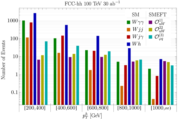
Figure 5: Number of SM and SMEFT events per $p_{T}^{h}$ bin after selection cuts for the signal and backgrounds at the FCC-hh assuming 30 ab^-1. The number of SMEFT events is obtained at the upper bound of the corresponding Wilson coefficients from a single operator fit with 5% syst.

Appendix B Chiral Perturbation Theory and Meson Decays

Below the QCD confinement scale, the light mesons are regarded as the pNGBs from the spontaneous breaking of the chiral symmetry by the quark condensation $\langle q_{L}^{\dagger}q_{R}\rangle\neq 0$. In the non-linear $\sigma$ model described by Chiral Perturbation Theory ($\chi$PT), the pNGBs are packaged into

$$U=\exp\left(\frac{i}{F_{\pi}}\pi^{a}\lambda^{a}\right)\;,$$ (37)

where $\lambda^{a},\;a=1\cdots 8$ are Gell-Mann matrices. Above the QCD scale, quarks are coupled to various spurions of the chiral symmetries, which provide additional building blocks for $\chi$PT Pich:2018ltt . At the two-quark level, one finds matrix-valued Lorentz scalar ($s,p$), vector ($v,a$) and tensor sources ($t$),

$${\cal L}_{\rm QCD}=\bar{q}\left(\gamma^{\mu}[v_{\mu}+\gamma_{5}a_{\mu}]-[s-i\gamma_{5}p]+\sigma^{\mu\nu}t_{\mu\nu}\right)q\ .$$ (38)

One also encounters the left/right equivalent of the vector/axial vector sources, $l_{\mu}\equiv v_{\mu}-a_{\mu},r_{\mu}\equiv v_{\mu}+a_{\mu}$. Other spurions appear at the four-quark level and higher orders.

B.1 $K\to\pi\pi$

The WET operator $\bar{s}\gamma^{\mu}dq\gamma_{\mu}q$ will induce the non-leptonic $K\rightarrow\pi\pi$ decay Buchalla:1995vs ; Gilman:1979bc . The decay rate can be computed via the chiral Lagrangian Cirigliano:2003gt ; Pich:2021yll ,

$$\mathcal{L}_{\rm weak}\supset-g_{8}GF_{\pi}^{4}\,\text{Tr}\left(P_{sd}L^{\mu}L_{\mu}\right)\;,$$ (39)

where $L_{\mu}=iU^{\dagger}D_{\mu}U$ and the covariant derivative $D^{\mu}U=\partial^{\mu}U-ir^{\mu}U+iUl^{\mu}$, and $P_{sd}\equiv\frac{1}{2}(\lambda_{6}-i\lambda_{7})$ projects onto the $s\rightarrow d$ transition. Following Ref. Pich:2021yll , the chiral Lagrangian parameter $g_{8}$ is determined by the WET Wilson coefficients $C_{i}$ defined in Eq. (13). For the operator ${\cal Q}_{q3}$ and its Wilson coefficient $C_{q3}$, to which the EW quark dipole SMEFT operator $\mathcal{O}_{uW}$ contributes at the weak scale as shown in Eq. (15), one finds,

$$\Delta g_{8}=\frac{\sqrt{2}\left(a_{8}^{S}-a_{8}^{A}\right)\Delta C_{q3}}{8V_{ud}V_{us}^{*}}\ ,$$ (40)

where $a_{8}^{S,A}$ are the numerical coefficients associated to the symmetric and antisymmetric combination of the chiral octets contained in $C_{q3}$ and can be computed with lattice methods. $\Delta C_{q3}$ is the contribution of $\mathcal{O}_{uW}$ which alters the parameter $g_{8}$. As shown in Fig. 3, the two-dipole insertion contributions to $C_{q3}$ are given by the same diagrams as for $C_{\ell 1}$, so that we find $\Delta C_{q3}=\Delta C_{\ell 1}$. The theoretical value of $g_{8}$, given by the Standard Model contribution to $C_{q3}$ and lattice simulations of $a_{8}^{S}=-0.20(24)$, $a_{8}^{A}=2.7(5)$, is $g_{8}^{\rm SM}=2.6(5)$ Pich:2021yll . On the other hand, through measurements of the $K\rightarrow\pi\pi$ decay amplitude, we can determine its experimental value as $g_{8}^{\rm exp}=3.07(14)$. Assuming that $g_{8}$ falls within $1\sigma$ of the difference $\Delta g_{8}=g_{8}^{\rm SM}-g_{8}^{\rm exp}=0.47(52)$, one establishes the following bound on the W-dipole Wilson coefficients,

$$|c_{uW}^{11}|\lesssim 13.2\left(\Lambda/\text{TeV}\right)^{2}\;.$$ (41)

As explained around Eq. (LABEL:eq:WETops), the EW quark dipole also contributes to the flavor-changing chromodipole Hurth:2019ula ,

$$\mathcal{O}_{8g}^{sd(\prime)}=g_{s}m_{s}\left[\bar{s}P_{R(L)}\sigma_{\mu\nu}T^{A}d\right]G_{A}^{\mu\nu}\;,$$ (42)

Its contribution to the $K\rightarrow\pi\pi$ hadronic matrix elements has been studied in Ref. Buras:2018evv , while its effect on the kaon direct CP violation is discussed in Ref. Chen:2018vog . Systematically exploring the FCNC effects of $\mathcal{O}_{8g}^{sd}$ could be a promising avenue that we leave for future research.

B.2 $\chi$PT with a Tensor Source

We discuss here the embedding in $\chi$PT of a tensor source which couples to quarks as follows,

$$\mathcal{L}=\bar{q}_{L}\sigma^{\mu\nu}t^{\dagger}_{\mu\nu}q_{R}+\bar{q}_{R}\sigma^{\mu\nu}t_{\mu\nu}q_{L}\;,$$ (43)

from which one reads its chiral transformation rules. In our case, where the tensor source arises from the SMEFT EW quark dipole, one finds at tree level,

$$t_{\mu\nu}=\frac{c_{uW}v_{h}}{\Lambda^{2}}P_{L}^{\mu\nu\lambda\rho}W_{\lambda\rho}\;,\quad P_{L}^{\mu\nu\lambda\rho}=\frac{1}{4}\left(g^{[\mu\lambda}g^{\nu]\rho}-i\varepsilon^{\mu\nu\lambda\rho}\right)\;.$$ (44)

The projector $P_{L}$ appears due to the relation $\sigma^{\mu\nu}\gamma_{5}=\frac{i}{2}\epsilon^{\lambda\rho\mu\nu}\sigma_{\lambda\rho}$. Following the notation in Ref. Cata:2007ns , it is also convenient to rewrite the chiral Lagrangian in terms of $\rho=\sqrt{U}$, and to trade the tensor source for the building blocks $t_{\pm}^{\mu\nu}$. Their definition, which can be extended to the field strengths $F_{L},F_{R}$ of the vector sources $l,r$, is as follows,

$$t_{\pm}^{\mu\nu}=\rho^{\dagger}t^{\mu\nu}\rho^{\dagger}\pm\rho t^{\mu\nu\dagger}\rho\;,\quad f_{\pm}^{\mu\nu}=\rho F_{L}^{\mu\nu}\rho^{\dagger}\pm\rho^{\dagger}F_{R}^{\mu\nu}\rho\;,$$ (45)

where $F_{L(R)}^{\mu\nu}=P_{L(R)}^{\mu\nu\lambda\rho}F_{\lambda\rho}$. One then finds that the chiral invariant operators at the lowest order are given by Cata:2007ns

$$\mathcal{L}^{\chi{\rm PT}}\supset c_{1}F_{0}\langle t_{+}^{\mu\nu}f_{+\mu\nu}\rangle+c_{2}F_{0}^{2}\langle t_{+}^{\mu\nu}t_{+\mu\nu}\rangle+c_{3}F_{0}^{2}\langle t_{+\mu\nu}\rangle^{2}\;,$$ (46)

where $\langle\cdots\rangle$ stands for the trace in the $u,d,s$ flavor space. As, in our case, $t_{+}^{\mu\nu}$ scales as $\Lambda^{-2}$, where $\Lambda$ is the SMEFT cutoff, the dominant contribution is given by the first term of Eq. (46).

Appendix C Other Effective Operators

As discussed in Sec. 2.2, in IHMFV, large left-handed FCNC may arise from the $LL$ type operators,

$$\bar{Q}_{L}\widetilde{Y}_{u}\widetilde{Y}_{u}^{\dagger}Q_{L}\;.$$ (47)

To check the size of these FCNC in the model of Sec. 5, which realizes IHMFV, we use Matchmakereft Carmona:2021xtq to compute the dimension-6 $Q_{L}Q_{L}$-type operators induced by $X$ at 1-loop and the result is,

$$\begin{aligned} &16\pi^{2}\frac{\text{Tr}(M_{X}M_{X}^{\dagger})}{\Lambda^{2}}\left[c_{\varphi q}^{(1)}\right]_{ij}=\frac{g_{1}^{2}}{90}\left[g_{1}^{2}+10|\lambda_{u}|^{2}\left(1-\ln\frac{M_{X}^{2}}{\mu^{2}}\right)\right]\delta_{ij}\;,\quad\\ &16\pi^{2}\frac{\text{Tr}(M_{X}M_{X}^{\dagger})}{\Lambda^{2}}\left[c_{\varphi q}^{(3)}\right]_{ij}=\frac{g_{2}^{2}}{30}\left(9g_{2}^{2}-5|\lambda_{u}|^{2}\right)\delta_{ij}\;,\\ &16\pi^{2}\frac{\text{Tr}(M_{X}M_{X}^{\dagger})}{\Lambda^{2}}\left[c_{qq}^{(1)}\right]_{ijk\ell}=-\frac{g_{3}^{4}}{30}\delta_{ij}\delta_{k\ell}+\frac{g_{1}^{4}}{540}\delta_{ij}\delta_{k\ell}\;,\\ &16\pi^{2}\frac{\text{Tr}(M_{X}M_{X}^{\dagger})}{\Lambda^{2}}\left[c_{qq}^{(3)}\right]_{ijk\ell}=-\frac{g_{3}^{4}}{10}\delta_{i\ell}\delta_{kj}-\frac{3g_{2}^{4}}{20}\delta_{ij}\delta_{k\ell}\;,\\ &16\pi^{2}\frac{\text{Tr}(M_{X}M_{X}^{\dagger})}{\Lambda^{2}}\left[c_{q\ell}^{(1)}\right]_{ijk\ell}=\frac{g_{1}^{4}}{90}\delta_{ij}\delta_{k\ell}\;,\quad\\ &16\pi^{2}\frac{\text{Tr}(M_{X}M_{X}^{\dagger})}{\Lambda^{2}}\left[c_{q\ell}^{(3)}\right]_{ijk\ell}=-\frac{3g_{2}^{4}}{10}\delta_{ij}\delta_{k\ell}\;,\\ &16\pi^{2}\frac{\text{Tr}(M_{X}M_{X}^{\dagger})}{\Lambda^{2}}\left[c_{qu}^{(1)}\right]_{ijk\ell}=-g_{1}^{2}\left[\frac{2g_{1}^{2}}{135}+\frac{|\lambda_{u}|^{2}}{648}\left(17-18\ln\frac{M_{X}^{2}}{\mu^{2}}\right)\right]\delta_{ij}\delta_{k\ell}\;,\\ &16\pi^{2}\frac{\text{Tr}(M_{X}M_{X}^{\dagger})}{\Lambda^{2}}\left[c_{qu}^{(8)}\right]_{ijk\ell}=-g_{3}^{2}\left[\frac{4g_{3}^{2}}{5}+\frac{8|\lambda_{u}|^{2}}{9}\right]\delta_{k\ell}\delta_{ij}\;,\\ &16\pi^{2}\frac{\text{Tr}(M_{X}M_{X}^{\dagger})}{\Lambda^{2}}\left[c_{qd}^{(1)}\right]_{ijk\ell}=\frac{g_{1}^{4}}{135}\delta_{ij}\delta_{k\ell}\;,\\ &16\pi^{2}\frac{\text{Tr}(M_{X}M_{X}^{\dagger})}{\Lambda^{2}}\left[c_{qd}^{(8)}\right]_{ijk\ell}=-\frac{4g_{3}^{4}}{5}\delta_{ij}\delta_{k\ell}\;,\\ &16\pi^{2}\frac{\text{Tr}(M_{X}M_{X}^{\dagger})}{\Lambda^{2}}\left[c_{qe}\right]_{ijk\ell}=\frac{g_{1}^{4}}{45}\delta_{ij}\delta_{k\ell}\;,\end{aligned}$$ (48)

where we have used the Fierz identity

$$\delta^{ij}\delta^{k\ell}\left(\bar{\psi}_{i}\gamma_{\mu}\psi_{j}\right)\left(\bar{\chi}_{k}\gamma^{\mu}\chi_{\ell}\right)=\delta^{ij}\delta^{k\ell}\left(\bar{\psi}_{i}\gamma_{\mu}\chi_{\ell}\right)\left(\bar{\chi}_{k}\gamma^{\mu}\psi_{j}\right)$$ (49)

to simplify the expressions. None of the $LL$-type operator in Eq. (LABEL:eq:LLWC) changes the quark flavor, because they are generated by the gauge interactions. This result can be understood from the diagrams relevant to the 1-loop matching after integrating out $X$, depicted in Fig. 6.

Figure 6: Feynman diagrams contributing to the one-loop matching between our UV model and the $LL$-type dimension-6 SMEFT operators, where $V_{\mu}=B_{\mu},\,W_{\mu}$. These diagrams preserve the flavor symmetry.

We can further explain the observed pattern as follows. In the model of Sec. 5, the two-point function of the field $X$ is the only source of the inverse Yukawa coupling, $\langle X\bar{X}\rangle\simeq\widetilde{Y}_{u}/M$. At one loop, one finds that large FCNC mediated by the operators in Eq. (47) can only be generated through the coupling between $\bar{Q}_{L}$, $X$ and another operator $\mathcal{O}$. The mass dimension of $\mathcal{O}$ in the renormalizable theory is 1 and we collectively denote the properties of $\mathcal{O}$ as,

$$\mathcal{L}\supset\widetilde{\lambda}\bar{Q}_{L}X\mathcal{O}\;,\quad[\mathcal{O}]=1\;.$$ (50)

The operator $\mathcal{O}$ can not be the mass mixing which is removable by the field redefinition. The only two candidates are the singlet scalar $S$ and and the gauge boson $V_{\mu}$ which appeared in the covariant derivative $D=\partial+igV$,

$$\mathcal{L}\supset\widetilde{\lambda}_{V}\bar{Q}_{L}\not{D}X+\widetilde{\lambda}_{S}\bar{Q}_{L}SX\;.$$ (51)

The first term does not mix quark flavors, because both the kinetic mixing and the mass mixing can be simultaneously eliminated through the rescaling and the rotation transformation. In the simple model of Eq. (32), the $U(1)_{M}$ symmetry forbids the $Q_{L}SX$ coupling. Then, there is no available field that can play the role of $\mathcal{O}$. In general, as long as interactions of the type in Eq. (50) are absent in the renormalizable UV model, the FCNC operators Eq. (47) will be suppressed in the IR EFT. We checked this in our model by computing all the dimension-6 effective operators and found that there are no $LL$-type flavor-violating operators.

References

- (1) W. Buchmuller and D. Wyler, “Effective Lagrangian Analysis of New Interactions and Flavor Conservation,” Nucl. Phys. B 268 (1986) 621–653.
- (2) B. Grzadkowski, M. Iskrzynski, M. Misiak, and J. Rosiek, “Dimension-Six Terms in the Standard Model Lagrangian,” JHEP 10 (2010) 085, arXiv:1008.4884 [hep-ph].
- (3) C. W. Murphy, “Dimension-8 operators in the Standard Model Eective Field Theory,” JHEP 10 (2020) 174, arXiv:2005.00059 [hep-ph].
- (4) H.-L. Li, Z. Ren, J. Shu, M.-L. Xiao, J.-H. Yu, and Y.-H. Zheng, “Complete set of dimension-eight operators in the standard model effective field theory,” Phys. Rev. D 104 no. 1, (2021) 015026, arXiv:2005.00008 [hep-ph].
- (5) H.-L. Li, Z. Ren, M.-L. Xiao, J.-H. Yu, and Y.-H. Zheng, “Complete set of dimension-nine operators in the standard model effective field theory,” Phys. Rev. D 104 no. 1, (2021) 015025, arXiv:2007.07899 [hep-ph].
- (6) R. V. Harlander, T. Kempkens, and M. C. Schaaf, “Standard model effective field theory up to mass dimension 12,” Phys. Rev. D 108 no. 5, (2023) 055020, arXiv:2305.06832 [hep-ph].
- (7) R. Alonso, E. E. Jenkins, and A. V. Manohar, “A Geometric Formulation of Higgs Effective Field Theory: Measuring the Curvature of Scalar Field Space,” Phys. Lett. B 754 (2016) 335–342, arXiv:1511.00724 [hep-ph].
- (8) A. Falkowski and R. Rattazzi, “Which EFT,” JHEP 10 (2019) 255, arXiv:1902.05936 [hep-ph].
- (9) T. Cohen, N. Craig, X. Lu, and D. Sutherland, “Is SMEFT Enough?,” JHEP 03 (2021) 237, arXiv:2008.08597 [hep-ph].
- (10) C. Arzt, M. B. Einhorn, and J. Wudka, “Patterns of deviation from the standard model,” Nucl. Phys. B 433 (1995) 41–66, arXiv:hep-ph/9405214.
- (11) M. B. Einhorn and J. Wudka, “The Bases of Effective Field Theories,” Nucl. Phys. B 876 (2013) 556–574, arXiv:1307.0478 [hep-ph].
- (12) N. Craig, M. Jiang, Y.-Y. Li, and D. Sutherland, “Loops and Trees in Generic EFTs,” JHEP 08 (2020) 086, arXiv:2001.00017 [hep-ph].
- (13) A. Adams, N. Arkani-Hamed, S. Dubovsky, A. Nicolis, and R. Rattazzi, “Causality, analyticity and an IR obstruction to UV completion,” JHEP 10 (2006) 014, arXiv:hep-th/0602178.
- (14) C. Zhang and S.-Y. Zhou, “Positivity bounds on vector boson scattering at the LHC,” Phys. Rev. D 100 no. 9, (2019) 095003, arXiv:1808.00010 [hep-ph].
- (15) G. N. Remmen and N. L. Rodd, “Consistency of the Standard Model Effective Field Theory,” JHEP 12 (2019) 032, arXiv:1908.09845 [hep-ph].
- (16) C. Zhang and S.-Y. Zhou, “Convex Geometry Perspective on the (Standard Model) Effective Field Theory Space,” Phys. Rev. Lett. 125 no. 20, (2020) 201601, arXiv:2005.03047 [hep-ph].
- (17) C. D. Froggatt and H. B. Nielsen, “Hierarchy of Quark Masses, Cabibbo Angles and CP Violation,” Nucl. Phys. B 147 (1979) 277–298.
- (18) M. Leurer, Y. Nir, and N. Seiberg, “Mass matrix models,” Nucl. Phys. B 398 (1993) 319–342, arXiv:hep-ph/9212278.
- (19) M. Leurer, Y. Nir, and N. Seiberg, “Mass matrix models: The Sequel,” Nucl. Phys. B 420 (1994) 468–504, arXiv:hep-ph/9310320.
- (20) N. Arkani-Hamed and M. Schmaltz, “Hierarchies without symmetries from extra dimensions,” Phys. Rev. D 61 (2000) 033005, arXiv:hep-ph/9903417.
- (21) Y. Grossman and M. Neubert, “Neutrino masses and mixings in nonfactorizable geometry,” Phys. Lett. B 474 (2000) 361–371, arXiv:hep-ph/9912408.
- (22) G. R. Dvali and M. A. Shifman, “Families as neighbors in extra dimension,” Phys. Lett. B 475 (2000) 295–302, arXiv:hep-ph/0001072.
- (23) T. Gherghetta and A. Pomarol, “Bulk fields and supersymmetry in a slice of AdS,” Nucl. Phys. B 586 (2000) 141–162, arXiv:hep-ph/0003129.
- (24) S. J. Huber and Q. Shafi, “Fermion masses, mixings and proton decay in a Randall-Sundrum model,” Phys. Lett. B 498 (2001) 256–262, arXiv:hep-ph/0010195.
- (25) A. E. Nelson and M. J. Strassler, “Suppressing flavor anarchy,” JHEP 09 (2000) 030, arXiv:hep-ph/0006251.
- (26) S. Davidson, G. Isidori, and S. Uhlig, “Solving the flavour problem with hierarchical fermion wave functions,” Phys. Lett. B 663 (2008) 73–79, arXiv:0711.3376 [hep-ph].
- (27) G. Isidori, “Effective Theories for Flavour Physics beyond the Standard Model,” PoS EFT09 (2009) 034, arXiv:0908.0404 [hep-ph].
- (28) A. Efrati, A. Falkowski, and Y. Soreq, “Electroweak constraints on flavorful effective theories,” JHEP 07 (2015) 018, arXiv:1503.07872 [hep-ph].
- (29) O. Aharony, L. Berdichevsky, M. Berkooz, Y. Hochberg, and D. Robles-Llana, “Inverted Sparticle Hierarchies from Natural Particle Hierarchies,” Phys. Rev. D 81 (2010) 085006, arXiv:1001.0637 [hep-ph].
- (30) C. Csaki, G. Perez, Z. Surujon, and A. Weiler, “Flavor Alignment via Shining in RS,” Phys. Rev. D 81 (2010) 075025, arXiv:0907.0474 [hep-ph].
- (31) M. Bordone, O. Catà, and T. Feldmann, “Effective Theory Approach to New Physics with Flavour: General Framework and a Leptoquark Example,” JHEP 01 (2020) 067, arXiv:1910.02641 [hep-ph].
- (32) D. A. Faroughy, G. Isidori, F. Wilsch, and K. Yamamoto, “Flavour symmetries in the SMEFT,” JHEP 08 (2020) 166, arXiv:2005.05366 [hep-ph].
- (33) A. Greljo, A. Palavrić, and A. E. Thomsen, “Adding Flavor to the SMEFT,” JHEP 10 (2022) 010, arXiv:2203.09561 [hep-ph].
- (34) F. Gabbiani, E. Gabrielli, A. Masiero, and L. Silvestrini, “A Complete analysis of FCNC and CP constraints in general SUSY extensions of the standard model,” Nucl. Phys. B 477 (1996) 321–352, arXiv:hep-ph/9604387.
- (35) UTfit Collaboration, M. Bona et al., “Model-independent constraints on operators and the scale of new physics,” JHEP 03 (2008) 049, arXiv:0707.0636 [hep-ph].
- (36) G. Isidori, Y. Nir, and G. Perez, “Flavor Physics Constraints for Physics Beyond the Standard Model,” Ann. Rev. Nucl. Part. Sci. 60 (2010) 355, arXiv:1002.0900 [hep-ph].
- (37) A. Crivellin, S. Najjari, and J. Rosiek, “Lepton Flavor Violation in the Standard Model with general Dimension-Six Operators,” JHEP 04 (2014) 167, arXiv:1312.0634 [hep-ph].
- (38) G. M. Pruna and A. Signer, “The decay in a systematic effective field theory approach with dimension 6 operators,” JHEP 10 (2014) 014, arXiv:1408.3565 [hep-ph].
- (39) F. Feruglio, “Theoretical Aspects of Flavour and CP Violation in the Lepton Sector,” in 27th Rencontres de Blois on Particle Physics and Cosmology. 9, 2015. arXiv:1509.08428 [hep-ph].
- (40) L. Silvestrini and M. Valli, “Model-independent Bounds on the Standard Model Effective Theory from Flavour Physics,” Phys. Lett. B 799 (2019) 135062, arXiv:1812.10913 [hep-ph].
- (41) J. Aebischer, C. Bobeth, A. J. Buras, and J. Kumar, “SMEFT ATLAS of F = 2 transitions,” JHEP 12 (2020) 187, arXiv:2009.07276 [hep-ph].
- (42) M. Ardu and S. Davidson, “What is Leading Order for LFV in SMEFT?,” JHEP 08 (2021) 002, arXiv:2103.07212 [hep-ph].
- (43) S. L. Glashow, J. Iliopoulos, and L. Maiani, “Weak Interactions with Lepton-Hadron Symmetry,” Phys. Rev. D 2 (1970) 1285–1292.
- (44) S. L. Glashow and S. Weinberg, “Natural Conservation Laws for Neutral Currents,” Phys. Rev. D 15 (1977) 1958.
- (45) R. S. Chivukula and H. Georgi, “Composite Technicolor Standard Model,” Phys. Lett. B 188 (1987) 99–104.
- (46) L. J. Hall and L. Randall, “Weak scale effective supersymmetry,” Phys. Rev. Lett. 65 (1990) 2939–2942.
- (47) A. J. Buras, P. Gambino, M. Gorbahn, S. Jager, and L. Silvestrini, “Universal unitarity triangle and physics beyond the standard model,” Phys. Lett. B 500 (2001) 161–167, arXiv:hep-ph/0007085.
- (48) G. D’Ambrosio, G. F. Giudice, G. Isidori, and A. Strumia, “Minimal flavor violation: An Effective field theory approach,” Nucl. Phys. B 645 (2002) 155–187, arXiv:hep-ph/0207036.
- (49) T. Feldmann and T. Mannel, “Large Top Mass and Non-Linear Representation of Flavour Symmetry,” Phys. Rev. Lett. 100 (2008) 171601, arXiv:0801.1802 [hep-ph].
- (50) A. L. Kagan, G. Perez, T. Volansky, and J. Zupan, “General Minimal Flavor Violation,” Phys. Rev. D 80 (2009) 076002, arXiv:0903.1794 [hep-ph].
- (51) K. Agashe, M. Papucci, G. Perez, and D. Pirjol, “Next to minimal flavor violation,” arXiv:hep-ph/0509117.
- (52) R. Barbieri, D. Buttazzo, F. Sala, and D. M. Straub, “Flavour physics from an approximate symmetry,” JHEP 07 (2012) 181, arXiv:1203.4218 [hep-ph].
- (53) G. Isidori and D. M. Straub, “Minimal Flavour Violation and Beyond,” Eur. Phys. J. C 72 (2012) 2103, arXiv:1202.0464 [hep-ph].
- (54) A. Antaramian, L. J. Hall, and A. Rasin, “Flavor changing interactions mediated by scalars at the weak scale,” Phys. Rev. Lett. 69 (1992) 1871–1873, arXiv:hep-ph/9206205.
- (55) L. J. Hall and S. Weinberg, “Flavor changing scalar interactions,” Phys. Rev. D 48 (1993) R979–R983, arXiv:hep-ph/9303241.
- (56) C. Degrande and J. Touchèque, “A reduced basis for CP violation in SMEFT at colliders and its application to diboson production,” JHEP 04 (2022) 032, arXiv:2110.02993 [hep-ph].
- (57) T. Kobayashi, H. Otsuka, M. Tanimoto, and K. Yamamoto, “Modular symmetry in the SMEFT,” Phys. Rev. D 105 no. 5, (2022) 055022, arXiv:2112.00493 [hep-ph].
- (58) S. Bar-Shalom and A. Rajaraman, “Models and phenomenology of maximal flavor violation,” Phys. Rev. D 77 (2008) 095011, arXiv:0711.3193 [hep-ph].
- (59) G. F. Giudice, B. Gripaios, and R. Sundrum, “Flavourful Production at Hadron Colliders,” JHEP 08 (2011) 055, arXiv:1105.3161 [hep-ph].
- (60) S. Knapen and D. J. Robinson, “Disentangling Mass and Mixing Hierarchies,” Phys. Rev. Lett. 115 no. 16, (2015) 161803, arXiv:1507.00009 [hep-ph].
- (61) D. Egana-Ugrinovic, S. Homiller, and P. Meade, “Aligned and Spontaneous Flavor Violation,” Phys. Rev. Lett. 123 no. 3, (2019) 031802, arXiv:1811.00017 [hep-ph].
- (62) A. Pich and P. Tuzon, “Yukawa Alignment in the Two-Higgs-Doublet Model,” Phys. Rev. D 80 (2009) 091702, arXiv:0908.1554 [hep-ph].
- (63) P. M. Ferreira, L. Lavoura, and J. P. Silva, “Renormalization-group constraints on Yukawa alignment in multi-Higgs-doublet models,” Phys. Lett. B 688 (2010) 341–344, arXiv:1001.2561 [hep-ph].
- (64) F. J. Botella, G. C. Branco, A. M. Coutinho, M. N. Rebelo, and J. I. Silva-Marcos, “Natural Quasi-Alignment with two Higgs Doublets and RGE Stability,” Eur. Phys. J. C 75 (2015) 286, arXiv:1501.07435 [hep-ph].
- (65) S. Gori, H. E. Haber, and E. Santos, “High scale flavor alignment in two-Higgs doublet models and its phenomenology,” JHEP 06 (2017) 110, arXiv:1703.05873 [hep-ph].
- (66) A. Peñuelas and A. Pich, “Flavour alignment in multi-Higgs-doublet models,” JHEP 12 (2017) 084, arXiv:1710.02040 [hep-ph].
- (67) W. Altmannshofer, S. Gori, D. J. Robinson, and D. Tuckler, “The Flavor-locked Flavorful Two Higgs Doublet Model,” JHEP 03 (2018) 129, arXiv:1712.01847 [hep-ph].
- (68) D. Egana-Ugrinovic, S. Homiller, and P. R. Meade, “Higgs bosons with large couplings to light quarks,” Phys. Rev. D 100 no. 11, (2019) 115041, arXiv:1908.11376 [hep-ph].
- (69) B. Batell, A. Freitas, A. Ismail, and D. Mckeen, “Flavor-specific scalar mediators,” Phys. Rev. D 98 no. 5, (2018) 055026, arXiv:1712.10022 [hep-ph].
- (70) B. Batell, A. Freitas, A. Ismail, D. McKeen, and M. Rai, “Renormalizable Models of Flavor-Specific Scalars,” arXiv:2107.08059 [hep-ph].
- (71) M. Pospelov and A. Ritz, “Electric dipole moments as probes of new physics,” Annals Phys. 318 (2005) 119–169, arXiv:hep-ph/0504231.
- (72) W. Dekens and J. de Vries, “Renormalization Group Running of Dimension-Six Sources of Parity and Time-Reversal Violation,” JHEP 05 (2013) 149, arXiv:1303.3156 [hep-ph].
- (73) G. Panico, A. Pomarol, and M. Riembau, “EFT approach to the electron Electric Dipole Moment at the two-loop level,” JHEP 04 (2019) 090, arXiv:1810.09413 [hep-ph].
- (74) J. Kley, T. Theil, E. Venturini, and A. Weiler, “Electric dipole moments at one-loop in the dimension-6 SMEFT,” Eur. Phys. J. C 82 no. 10, (2022) 926, arXiv:2109.15085 [hep-ph].
- (75) J. Brod, J. M. Cornell, D. Skodras, and E. Stamou, “Global constraints on Yukawa operators in the standard model effective theory,” JHEP 08 (2022) 294, arXiv:2203.03736 [hep-ph].
- (76) R. Alarcon et al., “Electric dipole moments and the search for new physics,” in Snowmass 2021. 3, 2022. arXiv:2203.08103 [hep-ph].
- (77) A. Falkowski, “Lectures on SMEFT,” Eur. Phys. J. C 83 no. 7, (2023) 656.
- (78) X.-G. He, G.-N. Li, and Y.-J. Zheng, “Probing Higgs boson Properties with at the LHC and the 100 TeV collider,” Int. J. Mod. Phys. A 30 no. 25, (2015) 1550156, arXiv:1501.00012 [hep-ph].
- (79) K. Hagiwara, H. Yokoya, and Y.-J. Zheng, “Probing the CP properties of top Yukawa coupling at an collider,” JHEP 02 (2018) 180, arXiv:1712.09953 [hep-ph].
- (80) J. Aebischer, C. Bobeth, A. J. Buras, J.-M. Gérard, and D. M. Straub, “Master formula for beyond the Standard Model,” Phys. Lett. B 792 (2019) 465–469, arXiv:1807.02520 [hep-ph].
- (81) J. Aebischer, C. Bobeth, A. J. Buras, and D. M. Straub, “Anatomy of beyond the standard model,” Eur. Phys. J. C 79 no. 3, (2019) 219, arXiv:1808.00466 [hep-ph].
- (82) E. Fuchs, M. Losada, Y. Nir, and Y. Viernik, “ violation from , and dimension-6 Yukawa couplings - interplay of baryogenesis, EDM and Higgs physics,” JHEP 05 (2020) 056, arXiv:2003.00099 [hep-ph].
- (83) H. Bahl, P. Bechtle, S. Heinemeyer, J. Katzy, T. Klingl, K. Peters, M. Saimpert, T. Stefaniak, and G. Weiglein, “Indirect probes of the Higgs-top-quark interaction: current LHC constraints and future opportunities,” JHEP 11 (2020) 127, arXiv:2007.08542 [hep-ph].
- (84) S. D. Bakshi, J. Chakrabortty, C. Englert, M. Spannowsky, and P. Stylianou, “Landscaping CP-violating BSM scenarios,” Nucl. Phys. B 975 (2022) 115676, arXiv:2103.15861 [hep-ph].
- (85) Q. Bonnefoy, E. Gendy, C. Grojean, and J. T. Ruderman, “Beyond Jarlskog: 699 invariants for CP violation in SMEFT,” JHEP 08 (2022) 032, arXiv:2112.03889 [hep-ph].
- (86) H. Bahl, E. Fuchs, S. Heinemeyer, J. Katzy, M. Menen, K. Peters, M. Saimpert, and G. Weiglein, “Constraining the structure of Higgs-fermion couplings with a global LHC fit, the electron EDM and baryogenesis,” Eur. Phys. J. C 82 no. 7, (2022) 604, arXiv:2202.11753 [hep-ph].
- (87) D. Kondo, H. Murayama, and R. Okabe, “23, 381, 6242, 103268, 1743183, … : Hilbert series for CP-violating operators in SMEFT,” JHEP 03 (2023) 107, arXiv:2212.02413 [hep-ph].
- (88) Q. Bonnefoy, E. Gendy, C. Grojean, and J. T. Ruderman, “Opportunistic CP violation,” JHEP 06 (2023) 141, arXiv:2302.07288 [hep-ph].
- (89) V. Barger, K. Hagiwara, and Y.-J. Zheng, “CP-violating top-Higgs coupling in SMEFT,” arXiv:2310.10852 [hep-ph].
- (90) M. Kobayashi and T. Maskawa, “CP Violation in the Renormalizable Theory of Weak Interaction,” Prog. Theor. Phys. 49 (1973) 652–657.
- (91) C. Jarlskog, “A Basis Independent Formulation of the Connection Between Quark Mass Matrices, CP Violation and Experiment,” Z. Phys. C 29 (1985) 491–497.
- (92) C. Jarlskog, “Commutator of the Quark Mass Matrices in the Standard Electroweak Model and a Measure of Maximal CP Nonconservation,” Phys. Rev. Lett. 55 (1985) 1039.
- (93) B. Grinstein, M. Redi, and G. Villadoro, “Low Scale Flavor Gauge Symmetries,” JHEP 11 (2010) 067, arXiv:1009.2049 [hep-ph].
- (94) R. Boughezal, E. Mereghetti, and F. Petriello, “Dilepton production in the SMEFT at ,” arXiv:2106.05337 [hep-ph].
- (95) L. Allwicher, D. A. Faroughy, F. Jaffredo, O. Sumensari, and F. Wilsch, “Drell-Yan tails beyond the Standard Model,” JHEP 03 (2023) 064, arXiv:2207.10714 [hep-ph].
- (96) F. Bishara, S. De Curtis, L. Delle Rose, P. Englert, C. Grojean, M. Montull, G. Panico, and A. N. Rossia, “Precision from the diphoton Zh channel at FCC-hh,” JHEP 04 (2021) 154, arXiv:2011.13941 [hep-ph].
- (97) F. Bishara, P. Englert, C. Grojean, G. Panico, and A. N. Rossia, “Revisiting Vh(→) at the LHC and FCC-hh,” JHEP 06 (2023) 077, arXiv:2208.11134 [hep-ph].
- (98) A. N. Rossia, M. O. A. Thomas, and E. Vryonidou, “Diboson production in the SMEFT from gluon fusion,” JHEP 11 (2023) 132, arXiv:2306.09963 [hep-ph].
- (99) J. Ellis, M. Madigan, K. Mimasu, V. Sanz, and T. You, “Top, Higgs, Diboson and Electroweak Fit to the Standard Model Effective Field Theory,” JHEP 04 (2021) 279, arXiv:2012.02779 [hep-ph].
- (100) SMEFiT Collaboration, J. J. Ethier, G. Magni, F. Maltoni, L. Mantani, E. R. Nocera, J. Rojo, E. Slade, E. Vryonidou, and C. Zhang, “Combined SMEFT interpretation of Higgs, diboson, and top quark data from the LHC,” JHEP 11 (2021) 089, arXiv:2105.00006 [hep-ph].
- (101) A. Azatov, R. Contino, C. S. Machado, and F. Riva, “Helicity selection rules and noninterference for BSM amplitudes,” Phys. Rev. D 95 no. 6, (2017) 065014, arXiv:1607.05236 [hep-ph].
- (102) D. Liu and L.-T. Wang, “Prospects for precision measurement of diboson processes in the semileptonic decay channel in future LHC runs,” Phys. Rev. D 99 no. 5, (2019) 055001, arXiv:1804.08688 [hep-ph].
- (103) J. Baglio, S. Dawson, S. Homiller, S. D. Lane, and I. M. Lewis, “Validity of standard model EFT studies of VH and VV production at NLO,” Phys. Rev. D 101 no. 11, (2020) 115004, arXiv:2003.07862 [hep-ph].
- (104) S. Banerjee, R. S. Gupta, J. Y. Reiness, S. Seth, and M. Spannowsky, “Towards the ultimate differential SMEFT analysis,” JHEP 09 (2020) 170, arXiv:1912.07628 [hep-ph].
- (105) F. Bishara, P. Englert, C. Grojean, M. Montull, G. Panico, and A. N. Rossia, “A New Precision Process at FCC-hh: the diphoton leptonic Wh channel,” JHEP 07 (2020) 075, arXiv:2004.06122 [hep-ph].
- (106) E. da Silva Almeida, N. Rosa-Agostinho, O. J. P. Éboli, and M. C. Gonzalez-Garcia, “Light-quark dipole operators at the LHC,” Phys. Rev. D 100 no. 1, (2019) 013003, arXiv:1905.05187 [hep-ph].
- (107) R. Escribano and E. Masso, “Constraints on fermion magnetic and electric moments from LEP-1,” Nucl. Phys. B 429 (1994) 19–32, arXiv:hep-ph/9403304.
- (108) G. Kopp, D. Schaile, M. Spira, and P. M. Zerwas, “Bounds on radii and magnetic dipole moments of quarks and leptons from LEP, SLC and HERA,” Z. Phys. C 65 (1995) 545–550, arXiv:hep-ph/9409457.
- (109) I. Brivio, T. Corbett, and M. Trott, “The Higgs width in the SMEFT,” JHEP 10 (2019) 056, arXiv:1906.06949 [hep-ph].
- (110) T. Corbett, O. J. P. Éboli, and M. C. Gonzalez-Garcia, “Unitarity Constraints on Dimension-Six Operators,” Phys. Rev. D 91 no. 3, (2015) 035014, arXiv:1411.5026 [hep-ph].
- (111) T. Corbett, O. J. P. Éboli, and M. C. Gonzalez-Garcia, “Unitarity Constraints on Dimension-six Operators II: Including Fermionic Operators,” Phys. Rev. D 96 no. 3, (2017) 035006, arXiv:1705.09294 [hep-ph].
- (112) T. Cohen, J. Doss, and X. Lu, “Unitarity bounds on effective field theories at the LHC,” JHEP 04 (2022) 155, arXiv:2111.09895 [hep-ph].
- (113) L. Di Luzio, J. F. Kamenik, and M. Nardecchia, “Implications of perturbative unitarity for scalar di-boson resonance searches at LHC,” Eur. Phys. J. C 77 no. 1, (2017) 30, arXiv:1604.05746 [hep-ph].
- (114) G. F. Giudice, C. Grojean, A. Pomarol, and R. Rattazzi, “The Strongly-Interacting Light Higgs,” JHEP 06 (2007) 045, arXiv:hep-ph/0703164.
- (115) A. Manohar and H. Georgi, “Chiral Quarks and the Nonrelativistic Quark Model,” Nucl. Phys. B 234 (1984) 189–212.
- (116) H. Georgi and L. Randall, “Flavor Conserving CP Violation in Invisible Axion Models,” Nucl. Phys. B 276 (1986) 241–252.
- (117) T. Corbett and A. Martin, “Higgs associated production with a vector decaying to two fermions in the geoSMEFT,” arXiv:2306.00053 [hep-ph].
- (118) E. E. Jenkins, A. V. Manohar, and P. Stoffer, “Low-Energy Effective Field Theory below the Electroweak Scale: Operators and Matching,” JHEP 03 (2018) 016, arXiv:1709.04486 [hep-ph]. [Erratum: JHEP 12, 043 (2023)].
- (119) E. E. Jenkins, A. V. Manohar, and P. Stoffer, “Low-Energy Effective Field Theory below the Electroweak Scale: Anomalous Dimensions,” JHEP 01 (2018) 084, arXiv:1711.05270 [hep-ph]. [Erratum: JHEP 12, 042 (2023)].
- (120) W. Dekens and P. Stoffer, “Low-energy effective field theory below the electroweak scale: matching at one loop,” JHEP 10 (2019) 197, arXiv:1908.05295 [hep-ph]. [Erratum: JHEP 11, 148 (2022)].
- (121) G. Buchalla, A. J. Buras, and M. E. Lautenbacher, “Weak decays beyond leading logarithms,” Rev. Mod. Phys. 68 (1996) 1125–1144, arXiv:hep-ph/9512380.
- (122) J. Aebischer, A. Crivellin, M. Fael, and C. Greub, “Matching of gauge invariant dimension-six operators for and transitions,” JHEP 05 (2016) 037, arXiv:1512.02830 [hep-ph].
- (123) A. Celis, J. Fuentes-Martin, A. Vicente, and J. Virto, “DsixTools: The Standard Model Effective Field Theory Toolkit,” Eur. Phys. J. C 77 no. 6, (2017) 405, arXiv:1704.04504 [hep-ph].
- (124) J. Aebischer, J. Kumar, and D. M. Straub, “Wilson: a Python package for the running and matching of Wilson coefficients above and below the electroweak scale,” Eur. Phys. J. C 78 no. 12, (2018) 1026, arXiv:1804.05033 [hep-ph].
- (125) T. Hurth, S. Renner, and W. Shepherd, “Matching for FCNC effects in the flavour-symmetric SMEFT,” JHEP 06 (2019) 029, arXiv:1903.00500 [hep-ph].
- (126) V. Cirigliano, G. Ecker, H. Neufeld, A. Pich, and J. Portoles, “Kaon Decays in the Standard Model,” Rev. Mod. Phys. 84 (2012) 399, arXiv:1107.6001 [hep-ph].
- (127) A. Pich and A. Rodríguez-Sánchez, “SU(3) analysis of four-quark operators: and vacuum matrix elements,” JHEP 06 (2021) 005, arXiv:2102.09308 [hep-ph].
- (128) J. Good, “Pion spectrum in radiative k + decay,” Physical Review 113 no. 1, (1959) 352.
- (129) M. Hoferichter, B.-L. Hoid, and J. R. de Elvira, “Improved Standard-Model prediction for ,” arXiv:2310.17689 [hep-ph].
- (130) Particle Data Group Collaboration, R. L. Workman, “Review of Particle Physics,” PTEP 2022 (2022) 083C01.
- (131) P. Mertens and C. Smith, “The s — d gamma decay in and beyond the Standard Model,” JHEP 08 (2011) 069, arXiv:1103.5992 [hep-ph].
- (132) P. V. Buividovich, M. N. Chernodub, E. V. Luschevskaya, and M. I. Polikarpov, “Lattice QCD in strong magnetic fields,” eCONF C0906083 (2009) 25, arXiv:0909.1808 [hep-ph].
- (133) O. Cata and V. Mateu, “Chiral perturbation theory with tensor sources,” JHEP 09 (2007) 078, arXiv:0705.2948 [hep-ph].
- (134) V. Mateu and J. Portoles, “Form-factors in radiative pion decay,” Eur. Phys. J. C 52 (2007) 325–338, arXiv:0706.1039 [hep-ph].
- (135) M. Jamin, “Flavor symmetry breaking of the quark condensate and chiral corrections to the Gell-Mann-Oakes-Renner relation,” Phys. Lett. B 538 (2002) 71–76, arXiv:hep-ph/0201174.
- (136) V. M. Belyaev and I. I. Kogan, “Supersymmetry and tensor coupling in decay,” Phys. Lett. B 280 (1992) 238–244.
- (137) V. N. Bolotov et al., “The Experimental study of the in flight,” Phys. Lett. B 243 (1990) 308–312.
- (138) V. Müller, “On the connection between the decays 0→ 2 and +→ e++ + ,” Zeitschrift für Physik 173 no. 4, (1963) 438–440.
- (139) R. Unterdorfer and H. Pichl, “On the Radiative Pion Decay,” Eur. Phys. J. C 55 (2008) 273–283, arXiv:0801.2482 [hep-ph].
- (140) J. Gasser and H. Leutwyler, “Chiral Perturbation Theory: Expansions in the Mass of the Strange Quark,” Nucl. Phys. B 250 (1985) 465–516.
- (141) J. Bijnens, G. Ecker, and J. Gasser, “Radiative semileptonic kaon decays,” Nucl. Phys. B 396 (1993) 81–118, arXiv:hep-ph/9209261.
- (142) M. Bychkov et al., “New Precise Measurement of the Pion Weak Form Factors in pi+ — e+ nu gamma Decay,” Phys. Rev. Lett. 103 (2009) 051802, arXiv:0804.1815 [hep-ex].
- (143) M. B. Voloshin, “On Compatibility of Small Mass with Large Magnetic Moment of Neutrino,” Sov. J. Nucl. Phys. 48 (1988) 512.
- (144) R. Franceschini, G. Panico, A. Pomarol, F. Riva, and A. Wulzer, “Electroweak Precision Tests in High-Energy Diboson Processes,” JHEP 02 (2018) 111, arXiv:1712.01310 [hep-ph].
- (145) J. Ellis, C. W. Murphy, V. Sanz, and T. You, “Updated Global SMEFT Fit to Higgs, Diboson and Electroweak Data,” JHEP 06 (2018) 146, arXiv:1803.03252 [hep-ph].
- (146) J. De Blas, G. Durieux, C. Grojean, J. Gu, and A. Paul, “On the future of Higgs, electroweak and diboson measurements at lepton colliders,” JHEP 12 (2019) 117, arXiv:1907.04311 [hep-ph].
- (147) J. Alwall, R. Frederix, S. Frixione, V. Hirschi, F. Maltoni, O. Mattelaer, H. S. Shao, T. Stelzer, P. Torrielli, and M. Zaro, “The automated computation of tree-level and next-to-leading order differential cross sections, and their matching to parton shower simulations,” JHEP 07 (2014) 079, arXiv:1405.0301 [hep-ph].
- (148) I. Brivio, “SMEFTsim 3.0 — a practical guide,” JHEP 04 (2021) 073, arXiv:2012.11343 [hep-ph].
- (149) A. Pich, “Effective Field Theory with Nambu-Goldstone Modes,” arXiv:1804.05664 [hep-ph].
- (150) F. J. Gilman and M. B. Wise, “Effective Hamiltonian for Delta s = 1 Weak Nonleptonic Decays in the Six Quark Model,” Phys. Rev. D 20 (1979) 2392.
- (151) V. Cirigliano, G. Ecker, H. Neufeld, and A. Pich, “Isospin breaking in K — pi pi decays,” Eur. Phys. J. C 33 (2004) 369–396, arXiv:hep-ph/0310351.
- (152) A. J. Buras and J.-M. Gérard, “ and Matrix Elements of the Chromomagnetic Operators from Dual QCD,” JHEP 07 (2018) 126, arXiv:1803.08052 [hep-ph].
- (153) C.-H. Chen and T. Nomura, “ from charged-Higgs-induced gluonic dipole operators,” Phys. Lett. B 787 (2018) 182–187, arXiv:1805.07522 [hep-ph].
- (154) A. Carmona, A. Lazopoulos, P. Olgoso, and J. Santiago, “Matchmakereft: automated tree-level and one-loop matching,” SciPost Phys. 12 no. 6, (2022) 198, arXiv:2112.10787 [hep-ph].