When Do We Not Need Larger Vision Models?

Abstract

Scaling up the size of vision models has been the de facto standard to obtain more powerful visual representations. In this work, we discuss the point beyond which larger vision models are not necessary. First, we demonstrate the power of Scaling on Scales (S²), whereby a pre-trained and frozen smaller vision model (e.g., ViT-B or ViT-L), run over multiple image scales, can outperform larger models (e.g., ViT-H or ViT-G) on classification, segmentation, depth estimation, Multimodal LLM (MLLM) benchmarks, and robotic manipulation. Notably, S² achieves state-of-the-art performance in detailed understanding of MLLM on the V^∗ benchmark, surpassing models such as GPT-4V. We examine the conditions under which S² is a preferred scaling approach compared to scaling on model size. While larger models have the advantage of better generalization on hard examples, we show that features of larger vision models can be well approximated by those of multi-scale smaller models. This suggests most, if not all, of the representations learned by current large pre-trained models can also be obtained from multi-scale smaller models. Our results show that a multi-scale smaller model has comparable learning capacity to a larger model, and pre-training smaller models with S² can match or even exceed the advantage of larger models. We release a Python package that can apply S² on any vision model with one line of code: https://github.com/bfshi/scaling_on_scales.

1 Introduction

Scaling up model size has been one of the key drivers of recent progress in various domains of artificial intelligence, including language modeling [8, 50, 69], image and video generation [79, 54, 34, 7], etc. Similarly, for visual understanding, larger models have consistently shown improvements across a wide range of downstream tasks given sufficient pre-training data [64, 82, 12, 49]. This trend has led to the pursuit of gigantic models with up to tens of billions of parameters as a default strategy for achieving more powerful visual representations and enhanced performance on downstream tasks [12, 18, 63, 22].

In this work, we revisit the question: Is a larger model always necessary for better visual understanding? Instead of scaling up model size, we consider scaling on the dimension of image scales—which we call Scaling on Scales (S²). With S², a pre-trained and frozen smaller vision model (e.g., ViT-B or ViT-L) is run on multiple image scales to generate a multi-scale representation. We take a model pre-trained on single image scale (e.g., $224^{2}$), interpolate the image to multiple scales (e.g., $224^{2}$, $448^{2}$, $672^{2}$), extract features on each scale by splitting larger images into sub-images of the regular size ($224^{2}$) and processing each separately before pooling them and concatenating with features from the original representation (Figure 1).

Surprisingly, from evaluations on visual representations of various pre-trained models (e.g., ViT [21], DINOv2 [49], OpenCLIP [12], MVP [53]), we show that smaller models with S² scaling consistently outperform larger models on classification, semantic segmentation, depth estimation, MLLM benchmarks, and robotic manipulation, with significantly fewer parameters ($0.28\times$ to $0.07\times$) and comparable GFLOPS. Remarkably, by scaling up image scale to $1008^{2}$, we achieve state-of-the-art performance in MLLM visual detail understanding on V^∗ benchmark [73], surpassing open-source and even commercial MLLMs like Gemini Pro [66] and GPT-4V [1].

We further examine conditions under which S² is a preferred scaling approach compared to model size scaling. We find that while smaller models with S² achieve better downstream performance than larger models in many scenarios, larger models can still exhibit superior generalization on hard examples. This prompts an investigation into whether smaller models can achieve the same level of generalization capability as larger ones. Surprisingly, we find that the features of larger models can be well approximated by multi-scale smaller models through a single linear transform, which means smaller models should have at least a similar learning capacity of their larger counterparts. We hypothesize that their weaker generalization stems from being pre-trained with single image scale only. Through experiments of ImageNet-21k pre-training on ViT, we show that pre-training with S² scaling improves the generalizability of smaller models, enabling them to match or even exceed the advantages of larger models.

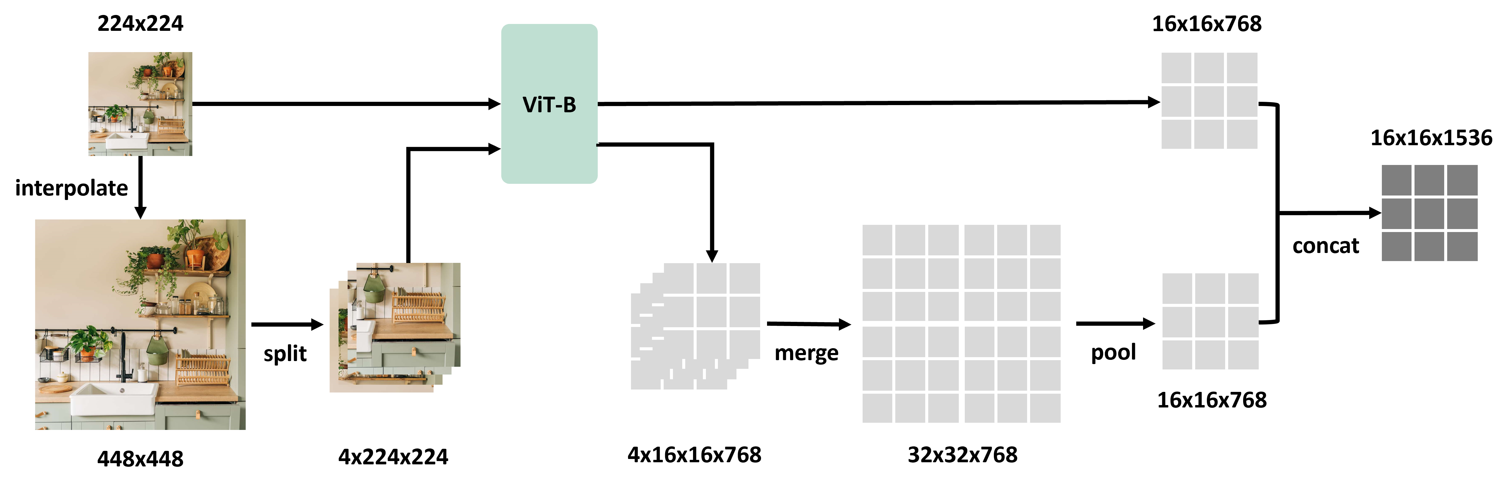
Figure 1: S²-Wrapper is a simple mechanism that extends any pre-trained vision model to multiple image scales in a parameter-free manner. Taking ViT-B as an example, S²-Wrapper first interpolates the input image to different scales (e.g., $224^{2}$ and $448^{2}$) and splits each into several sub-images of the same size as the default input size ($448^{2}$ $\rightarrow$ $4\times 224^{2}$). For each scale, all sub-images are fed into the same model and the outputs (e.g., $4\times 16^{2}$) are merged into feature map of the whole image ($32^{2}$). Feature maps of different scales are average-pooled to the original spatial size ($16^{2}$) and concatenated together. The final multi-scale feature has the same spatial shape as single-scale feature while having higher channel dimension (e.g., 1536 vs. 768).

2 Related Work

Multi-scale representation has been a common technique to recognize objects in a scale-invariant way since the era of feature engineering [19, 17, 44] and is later introduced into convolutional neural networks [70, 38, 56, 68] to extract features with both high-level semantics and low-level details. It has become a default test-time augmentation method for tasks such as detection and segmentation [14, 74], albeit at the cost of significantly slower inference speeds and typically limited image scales (up to $2\times$). Along with recent progress in vision transformers (ViT), variants of multi-scale ViTs [78, 23, 35, 9] as well as hierarchical ViTs [42, 58] have been proposed. However, these studies have not explored multi-scale representation as a general scaling approach as they usually design special architectures and are not applicable to common pre-trained vision models.

Scaling Vision Models. Training models with an increasing number of parameters has been the default approach to obtaining more powerful representations for visual pre-training [29, 43, 21, 49]. Previous research has studied how to optimally scale up vision models in terms of balancing model width, depth, and input resolution [64, 65, 4, 72, 20], although they are usually limited to convolutional networks or even specific architectures such as ResNet [29]. Recent work also explores model size scaling of vision transformers in various settings [12, 82, 18, 55]. Others have incorporated high-resolution images into pre-training [49, 24, 43, 42], although the maximum resolution typically does not exceed $512^{2}$ due to unbearable demands of computational resources. Hu et al. [32] study scaling on image scales through adjusting patch size for Masked Autoencoder (MAE) [30] where scaling is only applied on pre-training but not on downstream tasks.

3 The Power of Scaling on Scales

As an alternative to the conventional approach of scaling model size, we show the power of Scaling on Scales (S²), i.e., keeping the same size of a pre-trained model while running it on more and more image scales. From case studies on image classification, semantic segmentation, depth estimation, Multimodal LLMs, as well as robotic manipulation, we observe that S² scaling on a smaller vision model (e.g., ViT-B or ViT-L) often gives comparable or better performance than larger models (e.g., ViT-H or ViT-G), suggesting S² is a competitive scaling approach. In the following, we first introduce S²-Wrapper, a mechanism that extends any pre-trained frozen vision model to multiple image scales without additional parameters (Section 3.1). We then compare S² scaling and model size scaling in Section 3.2 - 3.3.

3.1 Scaling Pre-Trained Vision Models to Multiple Image Scales

We introduce S²-Wrapper, a parameter-free mechanism to enable multi-scale feature extraction on any pre-trained vision model. Regular vision models are normally pre-trained at a single image scale (e.g., $224^{2}$). S²-Wrapper extends a pre-trained model to multiple image scales (e.g., $224^{2}$, $448^{2}$) by splitting different scales of images to the same size as seen in pre-training. Specifically, given the image at $224^{2}$ and $448^{2}$ scales, S²-Wrapper first divides the $448^{2}$ image into four $224^{2}$ sub-images, which along with the original $224^{2}$ image are fed to the same pre-trained model. The features of four sub-images are merged back to the large feature map of the $448^{2}$ image, which is then average-pooled to the same size as the feature map of $224^{2}$ image. Output is the concatenation of feature maps across scales. The whole process is illustrated in Figure 1. Note that instead of directly using the $448^{2}$ resolution image, we obtain the $448^{2}$ image by interpolating the $224^{2}$ image. This is to make sure no additional high-resolution information is introduced so we can make a fair comparison with model size scaling which never sees the high-resolution image. For practitioners, directly using the high-resolution image is recommended.

There are several key designs that make S²-Wrapper efficient, effective, and easy to scale: (i) splitting the large image into small sub-images, instead of directly running on the whole large image, avoids quadratic computation complexity in self-attention and prevents performance degradation caused by position embedding interpolation [6], (ii) processing individual sub-images instead of using window attention allows using a pre-trained model that does not support window attention and avoids training additional parameters (e.g., relative position embedding) from scratch, (iii) interpolating the large feature map into the regular size makes sure the number of output tokens stays the same, preventing computational overhead in downstream applications such as MLLMs. Ablations of the designs can be found in Appendix. Note that we do not claim the novelty of extracting multi-scale features. Instead, we simply choose the most efficient and effective algorithm design and study its scaling property.

3.2 Scaling on Image Scales Can Beat Scaling on Model Size

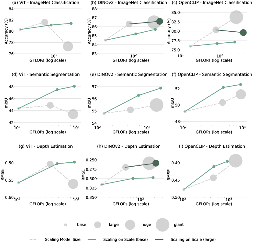
Figure 2: Comparison of S² scaling and model size scaling on three models (ViT, DINOv2, and OpenCLIP) and three tasks (ImageNet classification, semantic segmentation, and depth estimation). For each model and each task, we test base, large, and huge/giant models for model size scaling (plotted in gray curve). For S² scaling (plotted in green curve), we test three sets of scales from single-scale (1x) to multi-scale (up to 3x), and we adjust each set of scale so that it matches the GFLOPs of the respective model size. Note that for specific models and tasks, we test S² scaling on both base and large models (plotted in light green and dark green curves separately). We can see that in (a), (d), (e), (f), (g), and (i), the base model with S² scaling already achieves comparable or better performances than larger models with similar GFLOPs and much smaller model size. For (b), (h), S² scaling from the large model is comparable with the giant model, again with similar GFLOPs and fewer parameters. The only failure case is (c), where S² scaling on either base or large models does not compete with model size scaling.

S²-Wrapper enables S² scaling, i.e., keeping the same size of a pre-trained model while getting more and more powerful features by running on more and more image scales. Here we compare the scaling curve of S² to the regular approach of scaling up model size and show that S² scaling is a competitive, and in some cases, preferred scaling approach. To get a holistic analysis of two scaling approaches, we test their scaling curves on three representative tasks (image classification, semantic segmentation, and depth estimation) which correspond to the three dimensions of vision model capability [47], as well as on MLLMs and robotic manipulation which reflect the comprehensive ability of visual understanding.

Case study: image classification, semantic segmentation, and depth estimation. We use ImageNet [57], ADE20k [87], and NYUv2 [60] datasets for each task, respectively. We test on three families of pre-trained models (ViT [21], DINOv2 [49], and OpenCLIP [12]), spanning pre-training with different datasets (ImageNet-21k, LVD-142M, LAION-2B) and different pre-training objectives (supervised, unsupervised, and weakly-supervised). To see if the same observation holds for convolutional networks, we also test on ConvNeXt [43] (See Appendix). To fairly evaluate the representation learned from pre-training, we freeze the backbone and only train the task-specific head for all experiments. We use a single linear layer, Mask2former [10], and VPD depth decoder [85] as decoder heads for three tasks, respectively. For model size scaling, we test the performance of base, large, and huge or giant size of each model on each task. For S² scaling, we test three sets of scales including (1x), (1x, 2x), (1x, 2x, 3x). For example, for ViT on ImageNet classification, we use three sets of scales: ($224^{2}$), ($224^{2}$, $448^{2}$), and ($224^{2}$, $448^{2}$, $672^{2}$), which have the comparable GFLOPs as ViT-B, ViT-L, and ViT-H, respectively. Note that the scales for specific models and tasks are adjusted to match the GFLOPS of respective model sizes. The detailed configurations for each experiment can be found in Appendix.

The scaling curves are shown in Figure 2. We can see that in six out of nine cases ((a), (d), (e), (f), (g), (i)), S² scaling from base models gives a better scaling curve than model size scaling, outperforming large or giant models with similar GFLOPs and much fewer parameters. In two cases ((b) and (h)), S² scaling from base models has less competitive results than large models, but S² scaling from large models performs comparatively with giant models. The only failure case is (c) where both base and large models with S² scaling fail to compete with the giant model. Note that ViT-H is worse than ViT-L on all three tasks possibly due to the sub-optimal pre-training recipe [62]. We observe that S² scaling has more advantages on dense prediction tasks such as segmentation and depth estimation, which matches the intuition that multi-scale features can offer better detailed understanding which is especially required by these tasks. For image classification, S² scaling is sometimes worse than model size scaling (e.g., multi-scale DINOv2-B vs. DINOv2-L). We hypothesize this is due to the weak generalizability of the base model feature because we observe that the multi-scale base model has a lower training loss than the large model despite the worse performance, which indicates overfitting. In Section 4.3 we show that this can be fixed by pre-training with S² scaling as well.

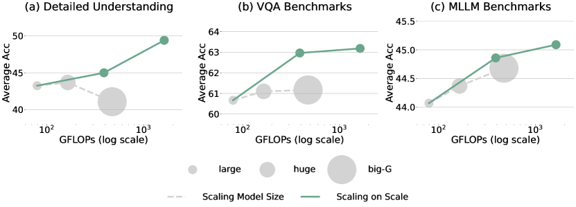
Figure 3: Comparison of S² scaling and model size scaling on MLLM. S² scaling has comparable or better scaling curve than model size scaling on all three types of benchmarks. Using large image scales consistently gives better performance while using larger model can degrade model performance in certain cases.

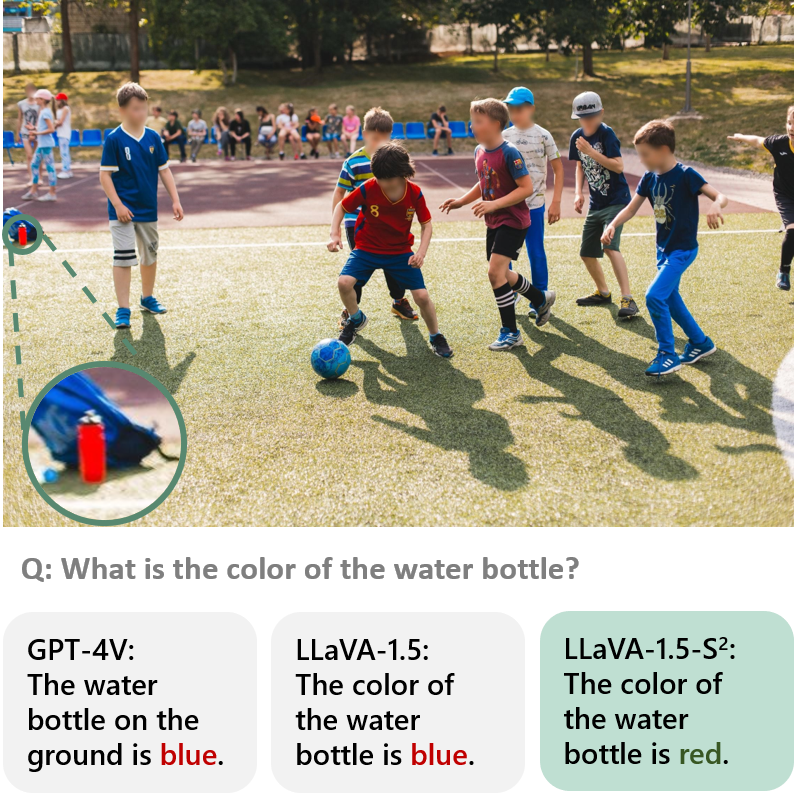
Figure 4: LLaVA-1.5 with S² scaling is able to recognize extremely fine-grained details in an image, e.g., the color of a bottle which only takes 23$\times$64 pixels in a $2250\times 1500$ image.

Table 1: S² scaling significantly improves the detailed understanding capability of LLaVA-1.5 on V^∗ benchmark, outperforming commercial models such as GPT-4V. Note that SEAL adopts visual searching which is about $10\times$ slower than S² ($6$s vs. $0.62$s) [73].

Model	Res.	#Tok	V${}^{\ast}_{\text{Att}}$	V${}^{\ast}_{\text{Spa}}$
Commercial or proprietary models
GPT-4V [1]	-	-	51.3	60.5
Gemini Pro [66]	-	-	40.9	59.2
Open-source models
SEAL [73]	-	-	74.8	76.3
InstructBLIP-7B [16]	224	-	25.2	47.4
Otter [36]	224	-	27.0	56.6
LLaVA-1.5-7B [39]	336	576	43.5	56.6
- S2 Scaling	1008	576	51.3	61.8
			(+7.8)	(+5.2)
LLaVA-1.5-13B [39]	336	576	41.7	55.3
- S2 Scaling	1008	576	50.4	63.2
			(+8.7)	(+7.9)

Case study: Multimodal LLMs. We compare S² scaling and model size scaling on MLLMs. We use a LLaVA [40]-style model where LLM is a Vicuna-7B [13] and the vision backbone is OpenCLIP. We keep the same LLM and only change the vision backbone. For model size scaling, we test vision model sizes of large, huge, and big-G. For S² scaling, we keep the large-size model and test scales of ($224^{2}$), ($224^{2}$, $448^{2}$), and ($224^{2}$, $448^{2}$, $896^{2}$). For all experiments, we keep the vision backbone frozen and only train a projector layer between the vision feature and LLM input space as well as a LoRA [31] on LLM. We follow the same training recipe as in LLaVA-1.5 [39]. We evaluate three types of benchmarks: (i) visual detail understanding (V^∗ [73]), (ii) VQA benchmarks (VQAv2 [27], TextVQA [61], VizWiz [28]), and (iii) MLLM benchmarks (MMMU [81], MathVista [45], MMBench [41], SEED-Bench [37], MM-Vet [80]).

A comparison of the two scaling approaches is shown in Figure 3. We report the average accuracy on each type of benchmarks. We can see that on all three types of benchmarks, S² scaling on large-size models performs better than larger models, using similar GFLOPs and much smaller model sizes. Especially, scaling to $896^{2}$ improves the accuracy of detailed understanding by about $6\%$. On all benchmarks, larger image scales consistently improve performance while bigger models sometimes fail to improve or even hurt performance. These results suggest S² is a preferable scaling approach for vision understanding in MLLMs as well.

We also observe that LLaVA-1.5, when equipped with S² scaling, is already competitive or better than state-of-the-art open-source and even commercial MLLMs. Results on visual detail understanding are shown in Table 1 and other results are available in Appendix. Here we use OpenAI CLIP [51] as the vision model for fair comparison. On visual detail understanding, LLaVA-1.5 with S² scaling outperforms all other open-source MLLMs as well as commercial models such as Gemini Pro and GPT-4V. This is credited to the highly fine-grained features we are able to extract by scaling image resolution to $1008^{2}$. A qualitative example is shown in Figure 4. We can see that LLaVA-1.5 with S² is able to recognize an extremely small object that only takes $23\times 64$ pixels in a $2250\times 1500$ image and correctly answer the question about it. In the meantime, both GPT-4V and LLaVA-1.5 fail to give the correct answer. In contrast to previous experiments, here we directly use the high-resolution image instead of interpolating from the low-resolution image in order to compare with the state of the arts. Note that despite the large image scale, we keep the same number of image tokens as baseline LLaVA-1.5 since we interpolate the feature map of the large-scale images to the same size as that of the original image (see Section 3.1). This makes sure the context length (and thus the computational cost) of LLM does not increase when using larger image scales, allowing us to use much higher resolution than the baselines.

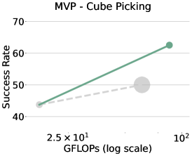
Figure 5: S² vs. model size scaling on cube picking task. S² scaling on base-size model improves the success rate by about $20\%$.

Case study: robotic manipulation. We compare S² and model size scaling on a robotic manipulation task of cube picking. The task requires controlling a robot arm to pick up a cube on the table. We train a vision-based end-to-end policy on 120 demos using behavior cloning, and evaluate the success rate of picking on 16 randomly chosen cube positions, following the setting in [52]. We use MVP [53] as the pre-trained vision encoder to extract visual features which are fed to the policy. Please refer to Appendix for the detailed setting. To compare S² and model size scaling, we evaluate base and large models with single scale of ($224^{2}$), as well as a multi-scale base model with scales of ($224^{2}$, $448^{2}$). Results are shown in Figure 5. Scaling from base to large model improves the success rate by about $6\%$, while scaling to larger image scales improves the success rate by about $20\%$. This demonstrates the advantage of S² over model size scaling on robotic manipulation tasks as well.

3.3 The Sweet Spot Between Model Size Scaling and S² Scaling

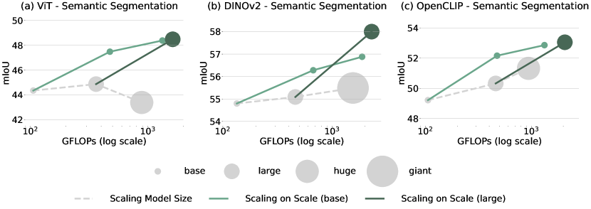
Figure 6: Which model size should we scale up image scales on? The answer varies for different pre-trained models. For ViT and OpenCLIP, S² scaling from base or large model gives similar performances under computation budget beyond the huge-size model while the former performs better under similar GFLOPS as the large-size model. For DINOv2, S² scaling from the large size model has better performance than scaling from base size, especially under the same level of computation budget as the giant-size model.

While S² scaling outperforms model size scaling on a wide range of downstream tasks, a natural question arises: on which model size should we perform S² scaling? We show that it depends on different pre-trained models. For certain models, S² scaling from a large-size model gives an even better scaling curve when S² scaling from base model already beats larger models. As an example, we compare S² scaling from base and large models on semantic segmentation for ViT, DINOv2, and OpenCLIP. Results are shown in Figure 6. We can see that for ViT and OpenCLIP, S² scaling from base models is better than from large models when the amount of computation is less than that of the huge-size models. These two curves eventually converge after going beyond the GFLOPs of the huge models. This means S² scaling from large models has no significant benefit than from base models. On the other hand, for DINOv2 we observe a clear advantage for S² scaling from the large model. When reaching the same level of GFLOPs as the giant-size model, S² scaling from the large model beats S² scaling from the base model by about 1 mIoU. These results indicate the optimal balancing between model size scaling and S² scaling varies for different models.

4 The (Non)Necessity of Scaling Model Size

Results from Section 3 suggest S² is a preferred scaling approach than model size scaling for various downstream scenarios. Nevertheless, larger vision models seem still necessary in certain cases (such as Figure 2(c)) where S² scaling cannot compete with model size scaling. In the following, we first study the advantage of larger models and show they usually generalize better on rare or hard instances than multi-scale smaller models (Section 4.1). Then, we explore if smaller models with S² scaling can achieve the same capability. We find that features of larger models can be well approximated by features of multi-scale smaller models, which means smaller models can learn what larger models learn to a large extent (Section 4.2). Based on this observation, we verify that multi-scale smaller models have similar capacity as larger models, and pre-training with S² scaling endows smaller models with similar or better generalization capability than larger models (Section 4.3).

4.1 Larger Models Generalize Better on Hard Examples

We use image classification as a testbed to understand the advantage of larger models. We conduct a qualitative analysis of what kinds of images are recognized better by a larger model but not by using larger image scales. Specifically, we find samples in ImageNet that a larger model (ViT-L) improves the most over a smaller model (ViT-B) but a multi-scale model (ViT-B-S²) fails to improve, as shown in Figure 7. For each sample, we also find two easy samples (which two models both recognize correctly) from the same class as a comparison. We can see that there are mainly two types of images that larger models have advantages on. The first type is rare samples. For example, a television or a flute but in the form of a sculpture instead of regular ones (Figure 7(a)). Larger models have larger capacity to learn to classify these rare examples during pre-training. The second type (Figure 7(b)) is ambiguous examples, where the object can belong to either category (e.g., lotion and soap dispenser), or there are two categories co-existing in the same image and both labels should be correct (e.g., airship and traffic light). In this case, despite multiple correct labels, the large model is able to remember the label presented in the dataset during pre-training. While the second type is due to the flawed labeling process of ImageNet which makes it an unfair comparison and does not imply any disadvantage of multi-scale smaller models [5, 48], the first type indicates larger model can generalize better on rare or hard cases.

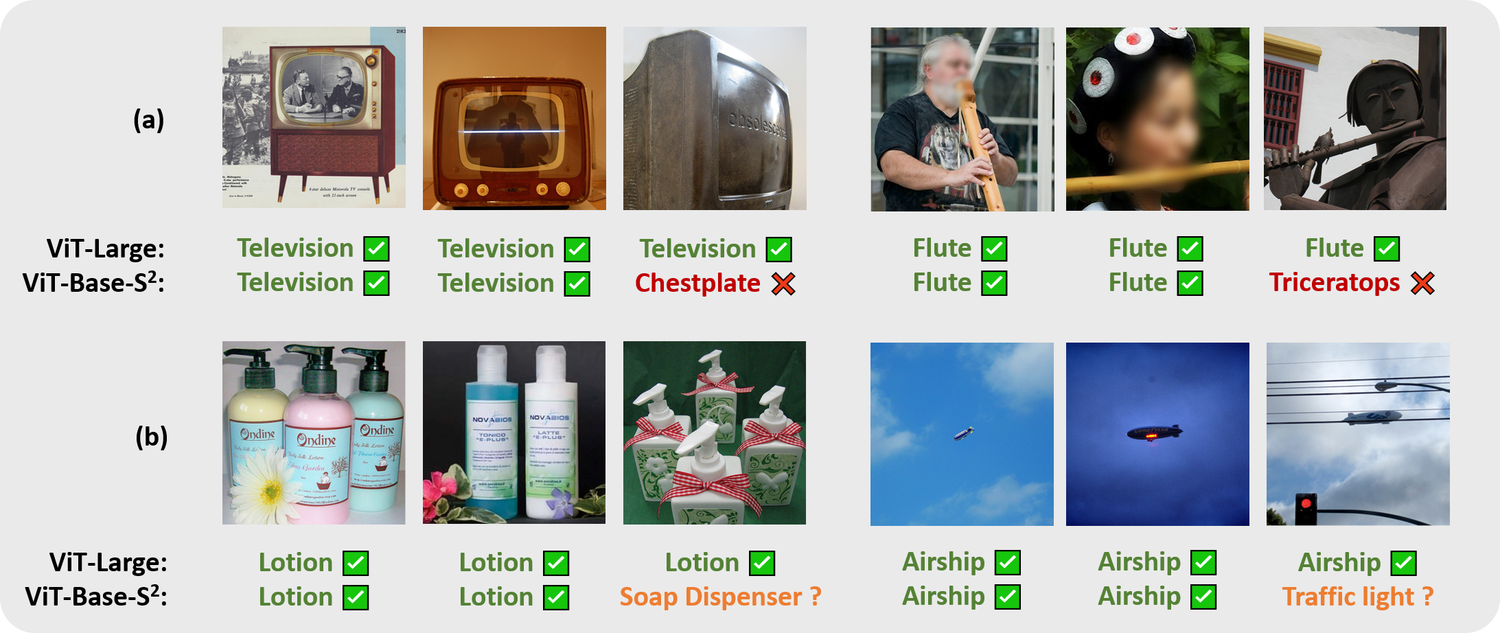
Figure 7: Types of samples that ViT-L improves the most but ViT-B-S² does not. (a) Rare cases. These samples clearly belong to the class but are hard to classify due to the rare appearance (e.g., sculptures of television and flute). (b) Ambiguous cases. These samples have ambiguous labels. For example, the lotion could also be soap dispenser due to their high similarity, or the label could be either airship or traffic light when these two objects co-exist.

4.2 Can Smaller Models Learn What Larger Models Learn?

Is the advantage of larger models due to some unique representation they have learned that smaller models cannot learn? We design experiments to study how much of the representation of larger models is also learned by multi-scale smaller models. Surprisingly, our preliminary results suggest that most, if not all, of the representation of larger models is also learned by multi-scale smaller models.

To quantify how much of the representation of a larger model (e.g., ViT-L) is also learned by a multi-scale smaller model (e.g., ViT-B-S²), we adopt a reconstruction-based evaluation, i.e., we train a linear transform to reconstruct the representation of a larger model from that of a multi-scale smaller model. Intuitively, low reconstruction loss means the representation of larger model can be equivalently learned by the multi-scale smaller model (through a linear transform) to a large extent. More formally, the reconstruction loss reflects the mutual information between two sets of representations. If we use MSE loss for reconstruction, the mutual information equals $I=-\log(l/l_{0})$, where $l$ is the reconstruction loss and $l_{0}$ is the loss of vanilla reconstruction where the large model representation is reconstructed by a dummy vector (See Appendix). This quantifies how much information in the larger model representation is also contained in the multi-scale smaller model. We use a linear transform for reconstruction to (i) account for operations that keep the representation equivalence (e.g., channel permutation), (ii) measure the information that is useful for downstream tasks considering the task decoders are usually light-weight modules such as a single linear layer [77].

Moreover, in practice we find the reconstruction loss is usually nowhere near zero. We hypothesize this is because part of the feature is non-reconstructable by nature, i.e., feature that is not relevant to the pre-training task and is learned due to randomness in weight initialization, optimization dynamics, etc., thus cannot be reconstructed from another model’s feature. To this end, we use an even larger (e.g., ViT-G) model to reconstruct the large model features as a comparison. Its reconstruction loss and corresponding mutual information are denoted by $l^{\ast}$ and $I^{\ast}=-\log(l^{\ast}/l_{0})$. If we assume that, when pre-trained on the same task and the same dataset, any task-relevant feature learned by a smaller model can also be learned by a larger model, then all the useful features in a large-size model should be reconstructable by a huge or giant model as well. This means $I^{\ast}$, the amount of information reconstructed from a huge or giant model, should serve as an upper bound of $I$. We empirically find this is indeed the case (see below). Therefore, we use the reconstruction ratio $I/I^{\ast}$ to measure how much representation in a larger model is also learned by a multi-scale smaller model.

We evaluate three classes of models: (i) ViT [21] pre-trained on ImageNet-21k, (ii) OpenCLIP [12] pre-trained on LAION-2B, and (iii) MAE [30] pre-trained on ImageNet-1k. Reconstruction loss is averaged over all output tokens and is evaluated on ImageNet-1k. Results are shown in Table 2. Compared to base models, we observe that multi-scale base models consistently have lower loss and reconstructs more information of the large model representation (e.g., 0.521 vs. 0.440 for ViT). More interestingly, we find that the amount of information reconstructed from a multi-scale base model is usually close to that of a huge or giant model, although sometimes slightly lower but never exceeding by a large margin. For example, while OpenCLIP-Base reconstructs $92.7\%$ of the information, the multi-scale base model can reconstruct $99.9\%$. For other models, the reconstruction ratio of Base-S² model is usually close to $100\%$ while never exceeding by more than $0.5\%$. This implies (i) huge/giant models are indeed a valid upper bound of feature reconstruction, and (ii) most part of the feature of larger models is also learned by multi-scale smaller models. The only exception is when we reconstruct OpenCLIP-Huge feature, the reconstruction ratio is $88.9\%$. Although it’s not near $100\%$, it is still significantly better than the base-size model which means at least a large part of the huge model feature is still multi-scale feature. These results imply smaller models with S² scaling should have at least a similar level of capacity to learn what larger models learn. On the other hand, we also notice that there exists a gap between train and test set, i.e., the reconstruction ratio on test set can be lower than train set (e.g. $96.3\%$ vs. $99.9\%$ on OpenCLIP-L). We hypothesize this is because we only apply multi-scale after pre-training and the base model feature pre-trained on single image scale only has weaker generalizability.

Table 2: Reconstructing representation of larger models from representation of regular or multi-scale smaller models. We test three classes of models (ViT, OpenCLIP, and MAE), and for each class we test base, multi-scale base (Base-S²), and huge or giant model. We report results on both training and test set of ImageNet-1k, and for each we report the reconstruction loss, the amount of information reconstructed, and the percentage of information reconstructed compared to huge or giant model.

Model Class	Target	Source	Train Set			Test Set
			Loss	Info	Ratio (%)	Loss	Info	Ratio (%)
ViT	Large	Base	0.1100	0.440	82.9%	0.0994	0.524	87.6%
		Base-S2	0.1040	0.521	98.1%	0.0942	0.601	100.5%
		Huge	0.1033	0.531	100%	0.0944	0.598	100%
MAE	Large	Base	0.0013	7.460	97.3%	0.0010	7.840	96.0%
		Base-S2	0.0011	7.694	100.3%	0.0009	7.972	97.6%
		Huge	0.001	7.669	100%	0.0008	8.169	100%
OpenCLIP	Large	Base	0.3693	1.495	92.7%	0.3413	1.723	90.7%
		Base-S2	0.3408	1.611	99.9%	0.3170	1.830	96.3%
		Giant	0.3402	1.613	100%	0.3022	1.900	100%
OpenCLIP	Huge	Base	0.3926	1.407	83.2%	0.4231	1.413	80.8%
		Base-S2	0.3670	1.504	88.9%	0.3970	1.505	86.0%
		Giant	0.3221	1.692	100%	0.3354	1.749	100%

4.3 Pre-Training With S² Makes Smaller Models Better

Given that most of the representation larger models have learned is also learned by multi-scale smaller models, we conjecture smaller models with S² scaling have at least similar capacity as larger models. Since larger capacity allows memorizing more rare and atypical instances during pre-training when given sufficient data and thus improves generalization error [25, 26, 46, 11, 3], we further speculate smaller models can achieve similar or even better generalizability than larger models if pre-trained with S² scaling as well. We verify these in the following.

Table 3: Training loss on instance memorization and image classification. A base model with S² scaling has similar memorization and classification losses, which implies it has at least the same level of model capacity as a large model.

Model	Mem. Loss	Cls. Loss (DINOv2)	Cls. Loss (OpenCLIP)
Base	1.223	3.855	4.396
Large	1.206	3.350	3.754
Base-S2	1.206	2.921	3.735

Table 4: Pre-training with S². Applying S² on a already pre-trained model has sub-optimal performance, while pre-training with S² makes smaller models better.

Model	Pre-train w/ S2	Acc. (ViT)	Acc. (DINOv2)
Base		80.3	77.6
Large		81.6	81.9
Base-S2	✗	81.1	78.4
Base-S2	✓	82.4	80.4

Multi-scale smaller models have similar capacity as larger models. To measure the model capacity, we use two surrogate metrics: (i) memorization capability, and (ii) training loss on a specific task. For memorization capability, given a dataset (e.g., ImageNet), we regard each image as a separate category and train the model to classify individual images, which requires the model to memorize every single image. The classification loss reflects how well each instance is memorized and thus the model capacity [83]. We adopt the training pipeline from [75]. For training loss, we report classification loss on the training set of ImageNet-1k for DINOv2 and OpenCLIP. Lower loss means the model fits the training data better, which implies a larger model capacity. Results are shown in Table 3. For instance memorization, we can see that ViT-B with S² scaling ($224^{2}$ and $448^{2}$) has a similar loss as ViT-L. For ImageNet classification, ViT-B-S² has a similar training loss as ViT-L for OpenCLIP, and an even lower loss for DINOv2. These results suggest that multi-scale smaller models have at least comparable model capacity as larger models.

Pre-training with S² makes smaller models better. We evaluate ImageNet classification of a base model scaled with S² either during pre-training or after pre-training. We pre-train the model on ImageNet-21k, using either ViT image classification or DINOv2 as the pre-training objective. We compare models with or without S² during pre-training with single-scale base and large models. Results are shown in Table 4. We can see that when the base models are trained with single image scale and only scaled to multiple image scales after pre-training, they have sub-optimal performances compared to the large models, which aligns with our observation in Section 3.2. However, when adding S² scaling into pre-training, the multi-scale base model is able to outperform the large model on ViT. For DINOv2, the base model pre-trained with S² achieves a performance that is significantly improved over the base model pre-trained without S², and is more comparable to the large model. Although it still slightly falls behind the large model, pre-training a large model with S² potentially can give a better scaling curve. These observations confirm our speculation that smaller models pre-trained with S² can match the advantage of larger models.

5 Discussion

In this work, we ask the question is a larger model always necessary for better visual understanding? We find that scaling on the dimension of image scales—which we call Scaling on Scales (S²)—instead of model size usually obtains better performance on a wide range of downstream tasks. We further show that smaller models with S² can learn most of what larger models learn, and pre-training smaller models with S² can match the advantage of larger models and even perform better. S² has a few implications for future work, including (i) scale-selective processing, i.e., not every scale at every position in an image contains equally useful features, and depending on image content and high-level task, it is much more efficient to select certain scales to process for each region, which resembles the bottom-up and top-down selection mechanism in human visual attention [86, 59, 33], (ii) parallel processing of single image, i.e., in contrast with regular ViT where the whole image is processed together at once, the fact that each sub-image is processed independently in S² enables parallel processing of different sub-images for a single image, which is especially helpful for scenarios where latency on processing single large images is critical [84].

Acknowledgements. We would like to thank Sheng Shen, Kumar Krishna Agrawal, Ritwik Gupta, Yossi Gandelsman, Chung Min Kim, Roei Herzig, Alexei Efros, Xudong Wang, and Ilija Radosavovic for their valuable discussions and suggestions on our project.

Appendix A Detailed Experimental Settings

The details of the models and the corresponding results on image classification, semantic segmentation, and depth estimation are listed in Table 5, 6, and 7, respectively. For each model type (ViT [21], DINOv2 [49], OpenCLIP [12]), we choose the scales so that the models with S² have comparable number of FLOPs with corresponding larger models. For image classification, we train a linear classifier for $30$ epochs with learning rate of $0.0005$ and batch size of $512$. For semantic segmentation, we train a Mask2Former decoder [10] following the configurations here. For depth estimation, we train a VPD depth decoder [85] following the configurations here.

Table 8 and 9 show the model details and full results for V^∗, VQA tasks, and MLLM benchmarks. We use OpenCLIP with large, huge, and big-G sizes, and also large-size model with $(224^{2})$, $(224^{2},448^{2})$, $(224^{2},448^{2},672^{2})$ scales. We follow the training and testing configurations in LLaVA-1.5. For evaluations on certain MLLM benchmarks such as MMMU [81], since it is not supported in the LLaVA-1.5 repo, we use VLMEvalKit [15] for evaluation.

Table 10 shows the model details and full results for the robotic manipulation task of cube picking. We use MVP [53] as the vision backbone and use base and large size as well as base size with $(224^{2},448^{2})$ scales. The vision backbone is frozen and extracts the visual feature for the visual observation at each time step. We train a transformer that takes in the visual features, proprioception and actions for the last 16 steps and outputs the actions for the next 16 steps. We train the model with behavior cloning on 120 self-collected demos. We test the model on 16 randomly selected cube positions and report the rate of successfully picking up the cube at these positions.

Table 5: Configurations of models and corresponding results on ImageNet classification.

	Model Size	Scales	#Params	#FLOPs	Acc.
ViT	Base	($224^{2}$)	86M	17.6G	80.3
	Base	($224^{2}$, $448^{2}$)	86M	88.1G	81.1
	Base	($224^{2}$, $448^{2}$, $672^{2}$)	86M	246.0G	81.4
	Large	($224^{2}$)	307M	61.6G	81.6
	Huge	($224^{2}$)	632M	204.9G	77.3
DINOv2	Base	($224^{2}$)	86M	22.6G	84.5
	Base	($224^{2}$, $448^{2}$)	86M	112.8G	85.2
	Base	($224^{2}$, $448^{2}$, $672^{2}$)	86M	315.9G	85.7
	Large	($224^{2}$)	303M	79.4G	86.3
	Large	($224^{2}$, $448^{2}$)	303M	397.1G	86.6
	Giant	($224^{2}$)	632M	295.4G	86.5
OpenCLIP	Base	($224^{2}$)	86M	17.6G	76.0
	Base	($224^{2}$, $448^{2}$)	86M	86.1G	76.7
	Base	($224^{2}$, $448^{2}$, $672^{2}$)	86M	241.0G	77.1
	Large	($224^{2}$)	303M	79.4G	80.4
	Large	($224^{2}$, $448^{2}$)	303M	397.1G	79.6
	Giant	($224^{2}$)	1012M	263.4G	83.8

Table 6: Configurations of models and corresponding results on ADE20k semantic segmentation.

	Model Size	Scales	#Params	#FLOPs	mIoU
ViT	Base	($512^{2}$)	86M	105.7G	44.4
	Base	($256^{2}$, $512^{2}$, $1024^{2}$)	86M	474.7G	47.8
	Base	($256^{2}$, $512^{2}$, $1536^{2}$)	86M	926.7G	48.0
	Large	($512^{2}$)	307M	362.1G	44.9
	Huge	($512^{2}$)	632M	886.2G	43.4
DINOv2	Base	($518^{2}$)	86M	134.4G	54.8
	Base	($518^{2}$, $1036^{2}$)	86M	671.8G	56.3
	Base	($518^{2}$, $1036^{2}$, $1554^{2}$)	86M	1881G	56.9
	Large	($518^{2}$)	303M	460.9G	55.1
	Giant	($518^{2}$)	632M	1553G	55.5
OpenCLIP	Base	($512^{2}$)	86M	105.7G	49.2
	Base	($256^{2}$, $512^{2}$, $1024^{2}$)	86M	474.7G	52.2
	Base	($256^{2}$, $512^{2}$, $1536^{2}$)	86M	926.7G	52.6
	Large	($518^{2}$)	303M	460.9G	50.3
	Huge	($518^{2}$)	632M	940.2G	51.3

Table 7: Configurations of models and corresponding results on NYUv2 depth estimation.

	Model Size	Scales	#Params	#FLOPs	RMSE
ViT	Base	($512^{2}$)	86M	105.7G	0.5575
	Base	($256^{2}$, $512^{2}$, $1024^{2}$)	86M	474.7G	0.5127
	Base	($256^{2}$, $512^{2}$, $1536^{2}$)	86M	926.7G	0.5079
	Large	($512^{2}$)	307M	362.1G	0.5084
	Huge	($512^{2}$)	632M	886.2G	0.5611
DINOv2	Base	($504^{2}$)	86M	134.4G	0.3160
	Base	($504^{2}$, $1008^{2}$)	86M	671.8G	0.2995
	Base	($504^{2}$, $1008^{2}$, $1512^{2}$)	86M	1881G	0.2976
	Large	($504^{2}$)	303M	460.9G	0.2696
	Large	($504^{2}$, $1008^{2}$)	303M	2170G	0.2584
	Giant	($504^{2}$)	632M	1553G	0.2588
OpenCLIP	Base	($512^{2}$)	86M	105.7G	0.4769
	Base	($256^{2}$, $512^{2}$, $1024^{2}$)	86M	474.7G	0.4107
	Base	($256^{2}$, $512^{2}$, $1536^{2}$)	86M	926.7G	0.3959
	Large	($504^{2}$)	303M	460.9G	0.4436
	Huge	($504^{2}$)	632M	940.2G	0.3939

Table 8: Configurations of models and corresponding results on V^∗ and VQA tasks.

	Model Size	Scales	#Params	#FLOPs	V${}^{\ast}_{\text{Att}}$	V${}^{\ast}_{\text{Spa}}$	VQA${}^{\text{v2}}$	VQA${}^{\text{T}}$	Viz
OpenCLIP	Large	($224^{2}$)	304M	79.4G	36.5	50.0	76.6	53.8	51.6
	Large	($224^{2}$, $448^{2}$)	304M	389.1G	40.0	50.0	77.8	55.9	55.2
	Large	($224^{2}$, $448^{2}$, $672^{2}$)	304M	1634G	35.7	63.2	77.9	56.5	55.3
	Huge	($224^{2}$)	632M	164.6G	37.4	50.0	76.0	54.0	53.3
	big-G	($224^{2}$)	1012M	473.4G	32.2	48.7	76.2	54.0	53.5

Table 9: Configurations of models and corresponding results on MLLM benchmarks.

	Model Size	Scales	#Params	#FLOPs	MMMU	Math	MMB	SEED	MMVet
OpenCLIP	Large	($224^{2}$)	304M	79.4G	35.4	24.0	64.2	65.5	31.6
	Large	($224^{2}$, $448^{2}$)	304M	389.1G	37.6	24.2	64.5	66.0	33.0
	Large	($224^{2}$, $448^{2}$, $672^{2}$)	304M	1634G	37.8	24.5	64.0	66.3	32.8
	Huge	($224^{2}$)	632M	164.6G	36.1	25.2	64.2	65.6	30.7
	big-G	($224^{2}$)	1012M	473.4G	35.6	25.2	64.8	65.1	32.8

Table 10: Configurations of models and corresponding results on robotic manipulation.

	Model Size	Scales	#Params	#FLOPs	Success Rate
MVP	Base	($224^{2}$)	86M	17.5G	43.8
	Base	($224^{2}$, $448^{2}$)	86M	87.9G	62.5
	Large	($224^{2}$)	307M	61.6G	50.0

Appendix B Derivation of Mutual Information

Denote the features from two models by ${\bm{x}}\in\mathbb{R}^{d_{x}}$ and ${\bm{y}}\in\mathbb{R}^{d_{y}}$ which follow the distribution $p({\mathbf{x}})$ and $p({\mathbf{y}})$, respectively. We make the simplest assumption that both the distribution and the conditional distribution of the features are isotropic gaussian distributions, i.e., $p({\mathbf{y}})\sim\mathcal{N}(\hat{{\bm{\mu}}},\sigma^{2}{\bm{I}})$ and $p({\mathbf{y}}|{\mathbf{x}})\sim\mathcal{N}(\hat{f}({\mathbf{x}}),\sigma^{\prime 2}{\bm{I}})$, where $f(\cdot)$ is a linear transform. The differential entropy and conditional differential entropy of ${\mathbf{y}}$ is $h({\mathbf{y}})=d_{y}\log\sigma+C$ and $h({\mathbf{y}}|{\mathbf{x}})=d_{y}\log\sigma^{\prime}+C$, where $C$ is a constant. The mutual information between features of two models is $I({\mathbf{x}};{\mathbf{y}})=h({\mathbf{y}})-h({\mathbf{y}}|{\mathbf{x}})=d_{y}\log\sigma-d_{y}\log\sigma^{\prime}$.

When reconstructing the features ${\mathbf{y}}$ from another model’s features ${\mathbf{x}}$, the optimal MSE loss would be $l=\min_{f}\frac{1}{d_{y}}E||{\mathbf{y}}-f({\mathbf{x}})||_{2}^{2}=\frac{1}{d_{y}}E||{\mathbf{y}}-\hat{f}({\mathbf{x}})||_{2}^{2}=\sigma^{\prime 2}$. The optimal MSE loss of reconstructing ${\mathbf{y}}$ from a dummy constant vector would be $l_{0}=\min_{\bm{\mu}}\frac{1}{d_{y}}E||{\mathbf{y}}-{\bm{\mu}}||_{2}^{2}=\frac{1}{d_{y}}E||{\mathbf{y}}-\hat{{\bm{\mu}}}||_{2}^{2}=\sigma^{2}$. Then we get the mutual information between ${\mathbf{x}}$ and ${\mathbf{y}}$ is $I({\mathbf{x}};{\mathbf{y}})=d_{y}\log\sigma-d_{y}\log\sigma^{\prime}=-\frac{d_{y}}{2}\log\frac{\sigma^{\prime 2}}{\sigma^{2}}\propto-\log\frac{l}{l_{0}}$.

Appendix C Results on ConvNeXt

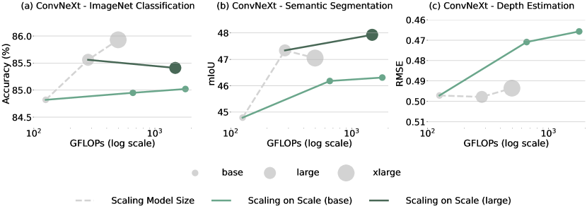
Figure 8: Comparison of S² scaling and model size scaling on ConvNeXt. We evaluate three tasks: ImageNet classification, semantic segmentation, and depth estimation. For S² scaling (plotted in green curve), we test three sets of scales from single-scale (1x) to multi-scale (up to 3x), and we adjust each set of scale so that it matches the GFLOPs of the respective model size. Note that for specific models and tasks, we test S² scaling on both base and large models (plotted in light green and dark green curves separately).

To see if convolutional networks have similar behaviors as transformer-based models, we test ConvNeXt [43] models (per-trained on ImageNet-21k) on three tasks: image classification, semantic segmentation, and depth estimation. We use ImageNet [57], ADE20k [87], and NYUv2 [60] datasets for each task. Similarly, we freeze the backbone and only train the task-specific head for all experiments, using a single linear layer, UPerNet [76], and VPD depth decoder [85] as the decoder heads for three tasks, respectively. For model size scaling, we test the base, large, and xlarge size performance of ConvNeXt [43] model on each task. For S² scaling, we test three sets of scales including (1x), (0.5x, 1x, 2x), and (0.5x, 1x, 2x, 3x).

The detailed curves are shown in Figure 8. We can see that in the depth estimation task (case (c)), S² scaling from base model significantly outperforms xlarge model with similar GFLOPs and only $0.25\times$ parameters. In the semantic segmentation task (case (b)), S² scaling from base model has less competitive result than larger models, while S² scaling from the large model outperforms the xlarge model with more GFLOPs but a smaller number of parameters. The ImageNet classification task (case (a)) is a failure case where S² scaling from both base and large model fail to compete with the xlarge model. From the observation above, we see that the convolutional networks show similar properties as transformer-based models: S² scaling has more advantages than model size scaling on dense prediction tasks such as segmentation and depth estimation while S² scaling is sometimes worse in image classification. This is possibly due to base and large model are not pre-trained with S² (see Section 4).

Appendix D Full Results on MLLM

Table 11: Full results on MLLM. We evaluate three types of benchmarks: visual detail understanding (V^∗ [73]), VQA benchmarks (VQAv2 [27], TextVQA [61], VizWiz [28]), and MLLM benchmarks (MMMU [81], MathVista [45], MMBench [41], SEED-Bench [37], MM-Vet [80]).

			Visual Detail		VQA Benchmarks			MLLM Benchmarks
Model	Res.	#Token	V${}^{\ast}_{\text{Att}}$	V${}^{\ast}_{\text{Spa}}$	VQA${}^{\text{v2}}$	VQA${}^{\text{T}}$	Viz	MMMU	Math	MMB	SEED	MMVet
Commercial or proprietary models
GPT-4V [1]	-	-	51.3	60.5	77.2	78.0	-	56.8	49.9	75.8	71.6	67.6
Gemini Pro [66]	-	-	40.9	59.2	71.2	74.6	-	47.9	45.2	73.6	70.7	64.3
Qwen-VL-Plus [67]	-	-	-	-	-	78.9	-	45.2	43.3	-	-	-
Open-source models
InstructBLIP-7B [16]	224	-	25.2	47.4	-	50.1	34.5	-	-	36.0	-	26.2
QwenVL-7B [2]	448	1024	-	-	78.8	63.8	35.2	-	-	38.2	-	-
QwenVL-Chat-7B [2]	448	1024	-	-	78.2	61.5	38.9	-	-	60.6	-	-
CogVLM-Chat [71]	490	1225	-	-	82.3	70.4	-	41.1	34.5	77.6	72.5	51.1
LLaVA-1.5-7B [39]	336	576	43.5	56.6	78.5	58.2	50.0	36.2	25.2	64.3	65.7	30.5
- S2 Scaling	1008	576	51.3	61.8	80.0	61.0	50.1	37.7	25.3	66.2	67.9	32.4
LLaVA-1.5-13B [39]	336	576	41.7	55.3	80.0	61.3	53.6	36.4	27.6	67.8	68.2	35.4
- S2 Scaling	1008	576	50.4	63.2	80.9	63.1	56.0	37.4	27.8	67.9	68.9	36.4

Full results on MLLM are shown in Table 11. We evaluate three types of benchmarks: visual detail understanding (V^∗ [73]), VQA benchmarks (VQAv2 [27], TextVQA [61], VizWiz [28]), and MLLM benchmarks (MMMU [81], MathVista [45], MMBench [41], SEED-Bench [37], MM-Vet [80]). We apply S² on LLaVA-1.5 to scale up the image resolution ot $1008^{2}$. Note that the cost of LLM inference is not changed because we are keeping the same number of visual tokens. The computational overhead completely comes from the vision encoder. S² scaling to $1008^{2}$ will add about $20\%$ - $30\%$ inference time for LLaVA-1.5. On V^∗, LLaVA-1.5 with S² scaling significantly improves over baselines, outperforming Gemini Pro and GPT-4V. On VQA and MLLM benchmarks, S² scaling consistently improves model performance as well. We observe that improvement on certain MLLM benchmarks such as MathVista is not as significant as others, which is probably because these benchmarks require strong mathematical or reasoning capabilities which is not achievable by only improving vision but needs stronger LLMs as well.

Appendix E Additional Qualitative Results on V^∗

We show more qualitative results on the V^∗ benchmark. We compare the performances of LLaVA-1.5 with S² scaling, original LLaVA-1.5 [39], and GPT-4V [1] on several examples in visual detail understanding (V^∗ [73]). Similarly, for LLaVa-1.5 with S² scaling, we use Vicuna-7B [13] as LLM and OpenAI CLIP as the vision backbone and apply S² scaling on the vision backbone.

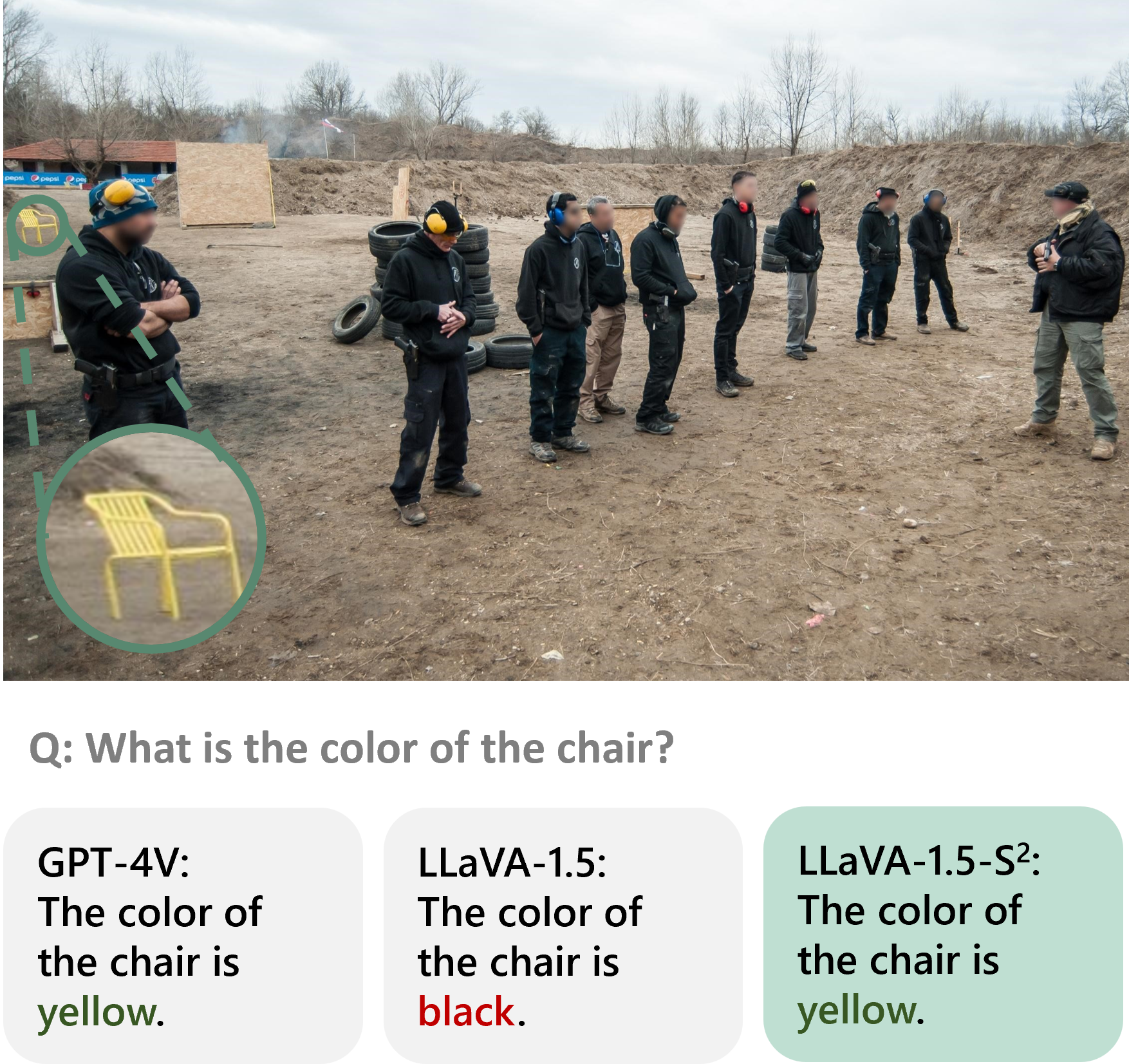
((a)) What is the color of the chair?

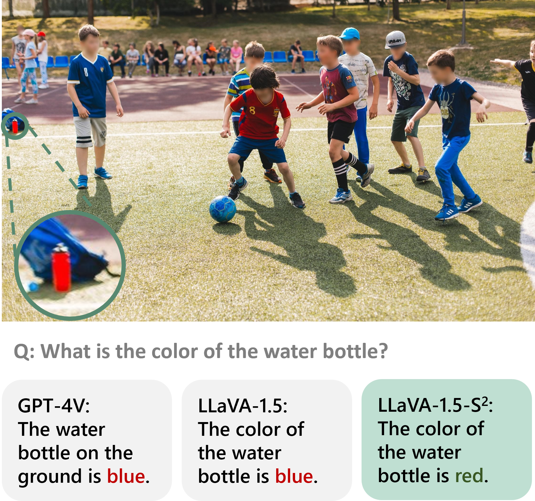
((b)) What is the color of the water bottle?

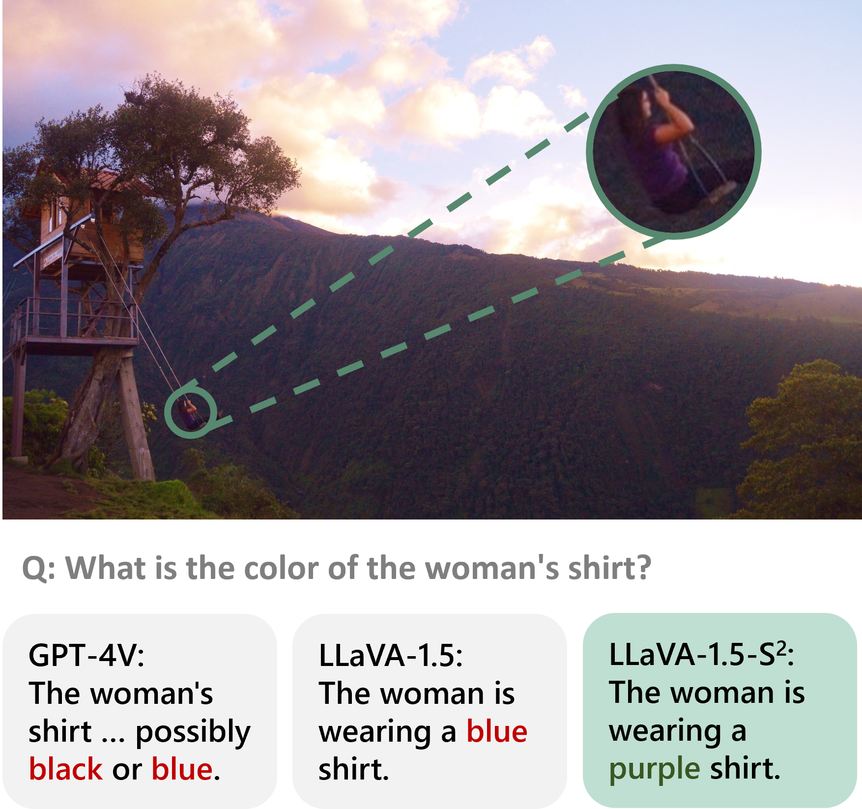
((c)) What is the color of the woman’s shirt?

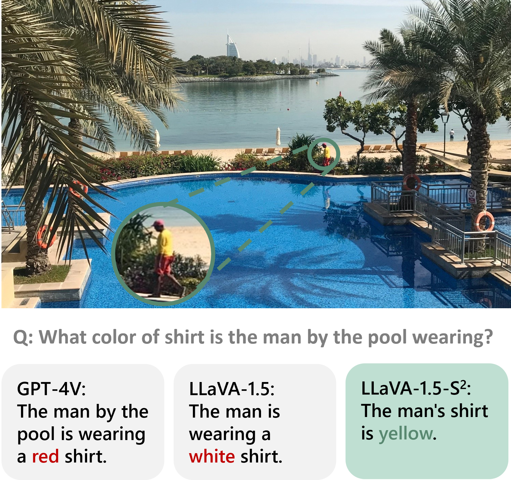
((d)) What color of shirt is the man by the pool wearing?

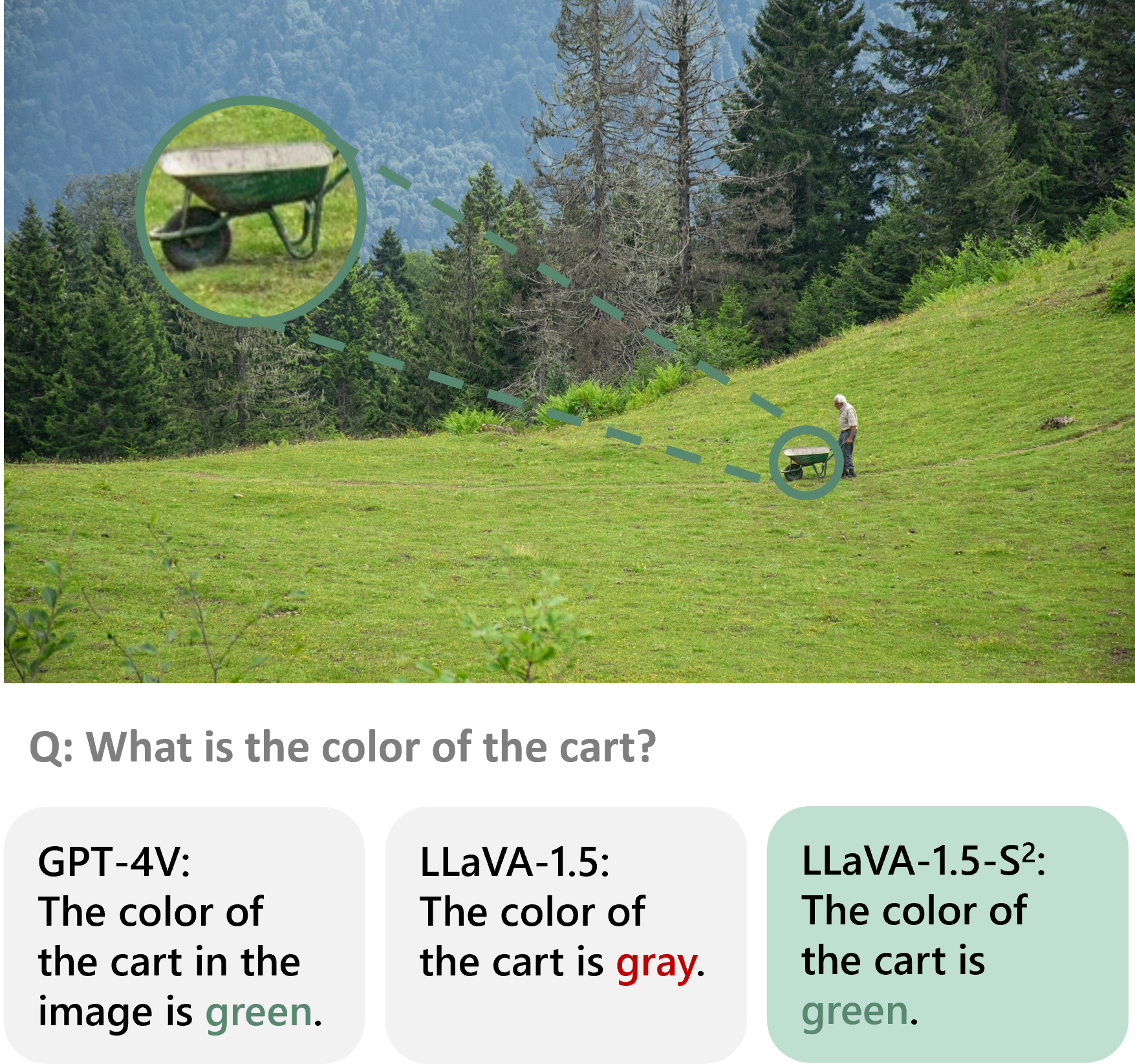
((e)) What is the color of the cart?

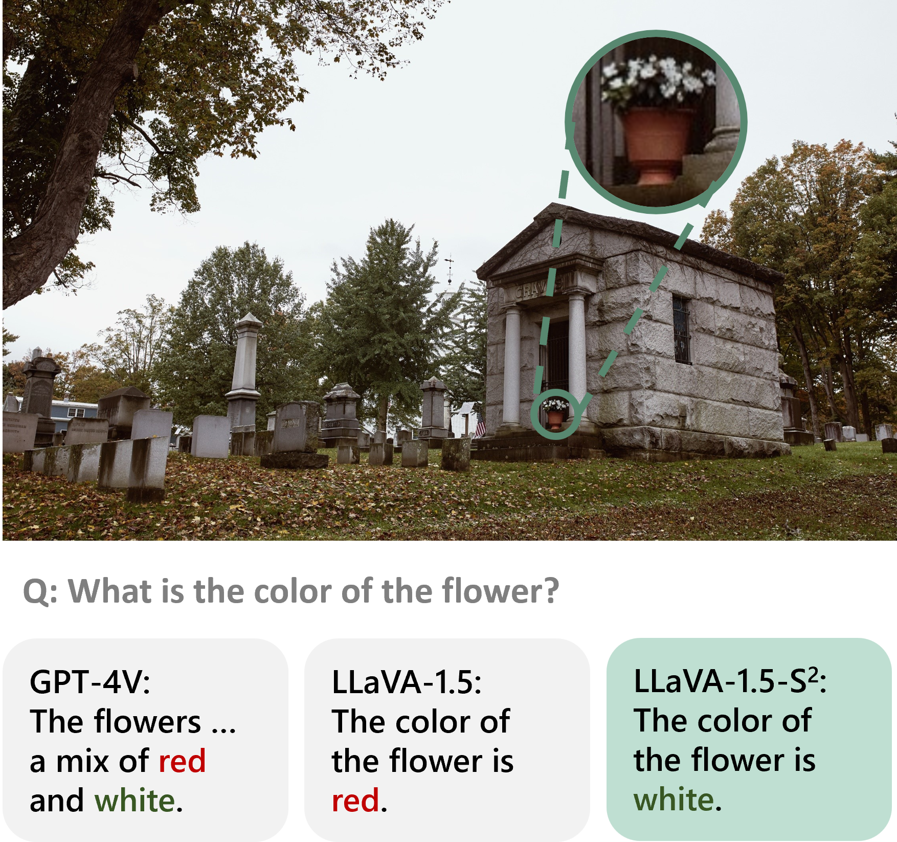
((f)) What is the color of the flower?

Figure 9: Examples of LLaVA-1.5 with S² scaling on the V^∗ benchmark, demonstrating its extreme ability in recognizing fine-grained details of an image.

In Figure 9, we see various examples that demonstrate the capabilities of different MLLMs. For instance, in example (f), the query is about the color of the flowers, which only occupy around 670 pixels in the $2550\times 1500$ image. Here, LLaVA-1.5-S² correctly identifies the color as ’white’. However, LLaVa-1.5 fails to capture the correct color and recognizes it as ’red’, which is actually the color of the flowerpot. On the other hand, GPT-4V recognizes the color as ’a mix of red and white’, indicating that it cannot distinguish the subtle differences between the flowerpot and flowers.

In another example (c), the query is about the color of the woman’s shirt. Here, the size of the woman’s figure is small, and the purple color of the shirt is very similar to the dark background color. In this case, LLaVA-1.5-S² correctly identifies the color of the shirt as ’purple’, while both LLaVA-1.5 and GPT-4V mistakenly identify the color of the shirt as ’black’ or ’blue’, which is the color of the background.

The above examples highlight the difference in performance between LLaVA-1.5-S², LLaVA-1.5 and GPT-4V. LLaVA-1.5-S² distinguishes itself through its heightened sensitivity and enhanced precision in visual detail understanding. This advanced level of detail recognition can be attributed to the S² scaling applied to its vision backbone, which significantly augments its ability to analyze and interpret subtle visual cues within complex images.

Appendix F Ablations of Model Design

We conduct the ablations on several designs of S²-Wrapper. Specifically, (i) we first compare running vision model on sub-images split from the large-scale image with running on the large-scale image directly, and then (ii) we compare concatenating feature maps from different scales with directly adding them together.

Results for (i) are shown in Table 12. We evaluate S²-Wrapper with or without image splitting on ADE20k semantic segmentation. We test base and large baselines, as well as multi-scale base model with (1x, 2x) and (1x, 2x, 3x) scales separately. We can see that for (1x, 2x) scales, image splitting has better results than no splitting, which is due to image splitting makes sure the input to the model has the same size as in pre-training, and avoids performance degradation caused by positional embedding interpolation when directly running on large images. However, note that even running directly on large images, multi-scale base model still has better results than base and large models, which indicates the effectiveness of S² scaling. Furthermore, image splitting enjoys higher computational efficiency because it avoids the quadratic complexity of self-attention. Notice that without image splitting, the training will run in OOM error when using (1x, 2x, 3x) scales.

Table 12: Ablation of splitting large-scale images. We compare splitting the large-scale image into regular-size sub-images vs. running the model directly on the large image. We evaluate on ADE20k semantic segmentation. We can see that S² scaling with image splitting consistently outperforms directly running on the large image while being more compute-efficient.

Model	Scales	Splitting	mIoU
Base	$518^{2}$		54.8
Large	$518^{2}$		55.1
Base-S2	$518^{2}$, $1036^{2}$	✗	55.7
Base-S2	$518^{2}$, $1036^{2}$	✓	56.3
Base-S2	$518^{2}$, $1036^{2}$, $1554^{2}$	✗	OOM
Base-S2	$518^{2}$, $1036^{2}$, $1554^{2}$	✓	56.9

Results for (ii) are shown in Table 13. We compare S²-Wrapper with concatenating features from different scales with directly adding the features. We evaluate on ADE20k semantic segmentation with DINOv2 and OpenCLIP. On both models, concatenating, as done by default in S²-Wrapper, has consistently better performance than adding the features.

Table 13: Ablation of how to merge features from different scales. We compare concatenating features with adding features from different scales. Concatenating has consistently better performance.

Model	Scales	Merging	mIoU
DINOv2-Base-S2	$518^{2}$, $1036^{2}$, $1536^{2}$	add	55.7
DINOv2-Base-S2	$518^{2}$, $1036^{2}$, $1536^{2}$	concat	56.9
OpenCLIP-Base-S2	$256^{2}$, $512^{2}$, $1024^{2}$	add	51.4
OpenCLIP-Base-S2	$256^{2}$, $512^{2}$, $1024^{2}$	concat	52.5

Appendix G Throughput of Models with S²

Previously we use FLOPs to measure the computational cost of different models. Since FLOPs is only a surrogate metric for the actual throughput of the models, here we compare the throughput of different models and verify if it aligns with FLOPs. Table 14 shows the results. We report the FLOPs and throughput put of DINOv2 model with base, large, and giant size, as well as base size with scales of $(1\times)$, $(1\times,2\times)$, and $(1\times,2\times,3\times)$. We test on base scales of $224^{2}$ and $518^{2}$. We can see that in general, the throughput follows the similar trends as FLOPs. For example, the base model with scales of ($224^{2}$, $448^{2}$, $672^{2}$) has the similar throughput as the giant model with scale of ($224^{2}$). The base model with scales of ($224^{2}$, $448^{2}$) has the about $0.8\times$ throughput as the large model with scale of ($224^{2}$). On base scale of $518^{2}$, the multi-scale base models with scales of $(1\times,2\times)$, and $(1\times,2\times,3\times)$ have about $0.7\times$ throughput as the large and giant models, respectively.

Table 14: Comparison of FLOPs and Throughput.

Model Size	Scales	#FLOPs	Throughput (image/s)
Base	($224^{2}$)	17.6G	138.5
Base	($224^{2}$, $448^{2}$)	88.1G	39.5
Base	($224^{2}$, $448^{2}$, $672^{2}$)	246.0G	16.5
Large	($224^{2}$)	61.6G	54.5
Giant	($224^{2}$)	204.9G	17.2
Base	($518^{2}$)	134.4G	34.9
Base	($518^{2}$, $1036^{2}$)	671.8G	7.7
Base	($518^{2}$, $1036^{2}$, $1554^{2}$)	1881G	2.7
Large	($518^{2}$)	460.9G	11.8
Giant	($518^{2}$)	1553G	3.8

References

- Achiam et al. [2023] Josh Achiam, Steven Adler, Sandhini Agarwal, Lama Ahmad, Ilge Akkaya, Florencia Leoni Aleman, Diogo Almeida, Janko Altenschmidt, Sam Altman, Shyamal Anadkat, et al. Gpt-4 technical report. arXiv preprint arXiv:2303.08774, 2023.
- Bai et al. [2023] Jinze Bai, Shuai Bai, Shusheng Yang, Shijie Wang, Sinan Tan, Peng Wang, Junyang Lin, Chang Zhou, and Jingren Zhou. Qwen-vl: A frontier large vision-language model with versatile abilities. arXiv preprint arXiv:2308.12966, 2023.
- Bartlett et al. [2020] Peter L Bartlett, Philip M Long, Gábor Lugosi, and Alexander Tsigler. Benign overfitting in linear regression. Proceedings of the National Academy of Sciences, 117(48):30063–30070, 2020.
- Bello et al. [2021] Irwan Bello, William Fedus, Xianzhi Du, Ekin Dogus Cubuk, Aravind Srinivas, Tsung-Yi Lin, Jonathon Shlens, and Barret Zoph. Revisiting resnets: Improved training and scaling strategies. Advances in Neural Information Processing Systems, 34:22614–22627, 2021.
- Beyer et al. [2020] Lucas Beyer, Olivier J Hénaff, Alexander Kolesnikov, Xiaohua Zhai, and Aäron van den Oord. Are we done with imagenet? arXiv preprint arXiv:2006.07159, 2020.
- Bolya et al. [2023] Daniel Bolya, Chaitanya Ryali, Judy Hoffman, and Christoph Feichtenhofer. Window attention is bugged: How not to interpolate position embeddings. arXiv preprint arXiv:2311.05613, 2023.
- Brooks et al. [2024] Tim Brooks, Bill Peebles, Connor Homes, Will DePue, Yufei Guo, Li Jing, David Schnurr, Joe Taylor, Troy Luhman, Eric Luhman, Clarence Ng, Ricky Wang, and Aditya Ramesh. Video generation models as world simulators. 2024. URL https://openai.com/research/video-generation-models-as-world-simulators.
- Brown et al. [2020] Tom Brown, Benjamin Mann, Nick Ryder, Melanie Subbiah, Jared D Kaplan, Prafulla Dhariwal, Arvind Neelakantan, Pranav Shyam, Girish Sastry, Amanda Askell, et al. Language models are few-shot learners. Advances in neural information processing systems, 33:1877–1901, 2020.
- Chen et al. [2021] Chun-Fu Richard Chen, Quanfu Fan, and Rameswar Panda. Crossvit: Cross-attention multi-scale vision transformer for image classification. In Proceedings of the IEEE/CVF international conference on computer vision, pages 357–366, 2021.
- Cheng et al. [2022a] Bowen Cheng, Ishan Misra, Alexander G Schwing, Alexander Kirillov, and Rohit Girdhar. Masked-attention mask transformer for universal image segmentation. In Proceedings of the IEEE/CVF conference on computer vision and pattern recognition, pages 1290–1299, 2022a.
- Cheng et al. [2022b] Chen Cheng, John Duchi, and Rohith Kuditipudi. Memorize to generalize: on the necessity of interpolation in high dimensional linear regression. In Conference on Learning Theory, pages 5528–5560. PMLR, 2022b.
- Cherti et al. [2023] Mehdi Cherti, Romain Beaumont, Ross Wightman, Mitchell Wortsman, Gabriel Ilharco, Cade Gordon, Christoph Schuhmann, Ludwig Schmidt, and Jenia Jitsev. Reproducible scaling laws for contrastive language-image learning. In Proceedings of the IEEE/CVF Conference on Computer Vision and Pattern Recognition, pages 2818–2829, 2023.
- Chiang et al. [2023] Wei-Lin Chiang, Zhuohan Li, Zi Lin, Ying Sheng, Zhanghao Wu, Hao Zhang, Lianmin Zheng, Siyuan Zhuang, Yonghao Zhuang, Joseph E Gonzalez, et al. Vicuna: An open-source chatbot impressing gpt-4 with 90%* chatgpt quality. See https://vicuna. lmsys. org (accessed 14 April 2023), 2023.
- Contributors [2020] MMSegmentation Contributors. MMSegmentation: Openmmlab semantic segmentation toolbox and benchmark. https://github.com/open-mmlab/mmsegmentation, 2020.
- Contributors [2023] OpenCompass Contributors. Opencompass: A universal evaluation platform for foundation models. https://github.com/open-compass/opencompass, 2023.
- Dai et al. [2023] Wenliang Dai, Junnan Li, Dongxu Li, Anthony Meng Huat Tiong, Junqi Zhao, Weisheng Wang, Boyang Li, Pascale Fung, and Steven Hoi. Instructblip: Towards general-purpose vision-language models with instruction tuning, 2023.
- Dalal and Triggs [2005] Navneet Dalal and Bill Triggs. Histograms of oriented gradients for human detection. In 2005 IEEE computer society conference on computer vision and pattern recognition (CVPR’05), volume 1, pages 886–893. Ieee, 2005.
- Dehghani et al. [2023] Mostafa Dehghani, Josip Djolonga, Basil Mustafa, Piotr Padlewski, Jonathan Heek, Justin Gilmer, Andreas Peter Steiner, Mathilde Caron, Robert Geirhos, Ibrahim Alabdulmohsin, et al. Scaling vision transformers to 22 billion parameters. In International Conference on Machine Learning, pages 7480–7512. PMLR, 2023.
- Dollár et al. [2014] Piotr Dollár, Ron Appel, Serge Belongie, and Pietro Perona. Fast feature pyramids for object detection. IEEE transactions on pattern analysis and machine intelligence, 36(8):1532–1545, 2014.
- Dollár et al. [2021] Piotr Dollár, Mannat Singh, and Ross Girshick. Fast and accurate model scaling. In Proceedings of the IEEE/CVF Conference on Computer Vision and Pattern Recognition, pages 924–932, 2021.
- Dosovitskiy et al. [2020] Alexey Dosovitskiy, Lucas Beyer, Alexander Kolesnikov, Dirk Weissenborn, Xiaohua Zhai, Thomas Unterthiner, Mostafa Dehghani, Matthias Minderer, Georg Heigold, Sylvain Gelly, et al. An image is worth 16x16 words: Transformers for image recognition at scale. arXiv preprint arXiv:2010.11929, 2020.
- El-Nouby et al. [2024] Alaaeldin El-Nouby, Michal Klein, Shuangfei Zhai, Miguel Angel Bautista, Alexander Toshev, Vaishaal Shankar, Joshua M Susskind, and Armand Joulin. Scalable pre-training of large autoregressive image models. arXiv preprint arXiv:2401.08541, 2024.
- Fan et al. [2021] Haoqi Fan, Bo Xiong, Karttikeya Mangalam, Yanghao Li, Zhicheng Yan, Jitendra Malik, and Christoph Feichtenhofer. Multiscale vision transformers. In Proceedings of the IEEE/CVF international conference on computer vision, pages 6824–6835, 2021.
- Fang et al. [2023] Yuxin Fang, Wen Wang, Binhui Xie, Quan Sun, Ledell Wu, Xinggang Wang, Tiejun Huang, Xinlong Wang, and Yue Cao. Eva: Exploring the limits of masked visual representation learning at scale. In Proceedings of the IEEE/CVF Conference on Computer Vision and Pattern Recognition, pages 19358–19369, 2023.
- Feldman [2020] Vitaly Feldman. Does learning require memorization? a short tale about a long tail. In Proceedings of the 52nd Annual ACM SIGACT Symposium on Theory of Computing, pages 954–959, 2020.
- Feldman and Zhang [2020] Vitaly Feldman and Chiyuan Zhang. What neural networks memorize and why: Discovering the long tail via influence estimation. Advances in Neural Information Processing Systems, 33:2881–2891, 2020.
- Goyal et al. [2017] Yash Goyal, Tejas Khot, Douglas Summers-Stay, Dhruv Batra, and Devi Parikh. Making the v in vqa matter: Elevating the role of image understanding in visual question answering. In Proceedings of the IEEE conference on computer vision and pattern recognition, pages 6904–6913, 2017.
- Gurari et al. [2018] Danna Gurari, Qing Li, Abigale J Stangl, Anhong Guo, Chi Lin, Kristen Grauman, Jiebo Luo, and Jeffrey P Bigham. Vizwiz grand challenge: Answering visual questions from blind people. In Proceedings of the IEEE conference on computer vision and pattern recognition, pages 3608–3617, 2018.
- He et al. [2016] Kaiming He, Xiangyu Zhang, Shaoqing Ren, and Jian Sun. Deep residual learning for image recognition. In Proceedings of the IEEE conference on computer vision and pattern recognition, pages 770–778, 2016.
- He et al. [2022] Kaiming He, Xinlei Chen, Saining Xie, Yanghao Li, Piotr Dollár, and Ross Girshick. Masked autoencoders are scalable vision learners. In Proceedings of the IEEE/CVF conference on computer vision and pattern recognition, pages 16000–16009, 2022.
- Hu et al. [2021] Edward J Hu, Yelong Shen, Phillip Wallis, Zeyuan Allen-Zhu, Yuanzhi Li, Shean Wang, Lu Wang, and Weizhu Chen. Lora: Low-rank adaptation of large language models. arXiv preprint arXiv:2106.09685, 2021.
- Hu et al. [2022] Ronghang Hu, Shoubhik Debnath, Saining Xie, and Xinlei Chen. Exploring long-sequence masked autoencoders. arXiv preprint arXiv:2210.07224, 2022.
- Itti and Koch [2001] Laurent Itti and Christof Koch. Computational modelling of visual attention. Nature reviews neuroscience, 2(3):194–203, 2001.
- Kondratyuk et al. [2023] Dan Kondratyuk, Lijun Yu, Xiuye Gu, José Lezama, Jonathan Huang, Rachel Hornung, Hartwig Adam, Hassan Akbari, Yair Alon, Vighnesh Birodkar, et al. Videopoet: A large language model for zero-shot video generation. arXiv preprint arXiv:2312.14125, 2023.
- Lee et al. [2022] Youngwan Lee, Jonghee Kim, Jeffrey Willette, and Sung Ju Hwang. Mpvit: Multi-path vision transformer for dense prediction. In Proceedings of the IEEE/CVF Conference on Computer Vision and Pattern Recognition, pages 7287–7296, 2022.
- Li et al. [2023a] Bo Li, Yuanhan Zhang, Liangyu Chen, Jinghao Wang, Fanyi Pu, Jingkang Yang, Chunyuan Li, and Ziwei Liu. Mimic-it: Multi-modal in-context instruction tuning. arXiv preprint arXiv:2306.05425, 2023a.
- Li et al. [2023b] Bohao Li, Rui Wang, Guangzhi Wang, Yuying Ge, Yixiao Ge, and Ying Shan. Seed-bench: Benchmarking multimodal llms with generative comprehension. arXiv preprint arXiv:2307.16125, 2023b.
- Lin et al. [2017] Tsung-Yi Lin, Piotr Dollár, Ross Girshick, Kaiming He, Bharath Hariharan, and Serge Belongie. Feature pyramid networks for object detection. In Proceedings of the IEEE conference on computer vision and pattern recognition, pages 2117–2125, 2017.
- Liu et al. [2023a] Haotian Liu, Chunyuan Li, Yuheng Li, and Yong Jae Lee. Improved baselines with visual instruction tuning. arXiv preprint arXiv:2310.03744, 2023a.
- Liu et al. [2023b] Haotian Liu, Chunyuan Li, Qingyang Wu, and Yong Jae Lee. Visual instruction tuning. arXiv preprint arXiv:2304.08485, 2023b.
- Liu et al. [2023c] Yuan Liu, Haodong Duan, Yuanhan Zhang, Bo Li, Songyang Zhang, Wangbo Zhao, Yike Yuan, Jiaqi Wang, Conghui He, Ziwei Liu, et al. Mmbench: Is your multi-modal model an all-around player? arXiv preprint arXiv:2307.06281, 2023c.
- Liu et al. [2021] Ze Liu, Yutong Lin, Yue Cao, Han Hu, Yixuan Wei, Zheng Zhang, Stephen Lin, and Baining Guo. Swin transformer: Hierarchical vision transformer using shifted windows. In Proceedings of the IEEE/CVF international conference on computer vision, pages 10012–10022, 2021.
- Liu et al. [2022] Zhuang Liu, Hanzi Mao, Chao-Yuan Wu, Christoph Feichtenhofer, Trevor Darrell, and Saining Xie. A convnet for the 2020s. In Proceedings of the IEEE/CVF conference on computer vision and pattern recognition, pages 11976–11986, 2022.
- Lowe [2004] David G Lowe. Distinctive image features from scale-invariant keypoints. International journal of computer vision, 60:91–110, 2004.
- Lu et al. [2023] Pan Lu, Hritik Bansal, Tony Xia, Jiacheng Liu, Chunyuan Li, Hannaneh Hajishirzi, Hao Cheng, Kai-Wei Chang, Michel Galley, and Jianfeng Gao. Mathvista: Evaluating mathematical reasoning of foundation models in visual contexts. arXiv preprint arXiv:2310.02255, 2023.
- Lukasik et al. [2023] Michal Lukasik, Vaishnavh Nagarajan, Ankit Singh Rawat, Aditya Krishna Menon, and Sanjiv Kumar. What do larger image classifiers memorise? arXiv preprint arXiv:2310.05337, 2023.
- Malik et al. [2016] Jitendra Malik, Pablo Arbeláez, Joao Carreira, Katerina Fragkiadaki, Ross Girshick, Georgia Gkioxari, Saurabh Gupta, Bharath Hariharan, Abhishek Kar, and Shubham Tulsiani. The three r’s of computer vision: Recognition, reconstruction and reorganization. Pattern Recognition Letters, 72:4–14, 2016.
- Northcutt et al. [2021] Curtis G Northcutt, Anish Athalye, and Jonas Mueller. Pervasive label errors in test sets destabilize machine learning benchmarks. arXiv preprint arXiv:2103.14749, 2021.
- Oquab et al. [2023] Maxime Oquab, Timothée Darcet, Théo Moutakanni, Huy Vo, Marc Szafraniec, Vasil Khalidov, Pierre Fernandez, Daniel Haziza, Francisco Massa, Alaaeldin El-Nouby, et al. Dinov2: Learning robust visual features without supervision. arXiv preprint arXiv:2304.07193, 2023.
- Radford et al. [2019] Alec Radford, Jeffrey Wu, Rewon Child, David Luan, Dario Amodei, Ilya Sutskever, et al. Language models are unsupervised multitask learners. OpenAI blog, 1(8):9, 2019.
- Radford et al. [2021] Alec Radford, Jong Wook Kim, Chris Hallacy, Aditya Ramesh, Gabriel Goh, Sandhini Agarwal, Girish Sastry, Amanda Askell, Pamela Mishkin, Jack Clark, et al. Learning transferable visual models from natural language supervision. In International conference on machine learning, pages 8748–8763. PMLR, 2021.
- Radosavovic et al. [2023a] Ilija Radosavovic, Baifeng Shi, Letian Fu, Ken Goldberg, Trevor Darrell, and Jitendra Malik. Robot learning with sensorimotor pre-training. arXiv preprint arXiv:2306.10007, 2023a.
- Radosavovic et al. [2023b] Ilija Radosavovic, Tete Xiao, Stephen James, Pieter Abbeel, Jitendra Malik, and Trevor Darrell. Real-world robot learning with masked visual pre-training. In Conference on Robot Learning, pages 416–426. PMLR, 2023b.
- Ramesh et al. [2022] Aditya Ramesh, Prafulla Dhariwal, Alex Nichol, Casey Chu, and Mark Chen. Hierarchical text-conditional image generation with clip latents. arXiv preprint arXiv:2204.06125, 1(2):3, 2022.
- Riquelme et al. [2021] Carlos Riquelme, Joan Puigcerver, Basil Mustafa, Maxim Neumann, Rodolphe Jenatton, André Susano Pinto, Daniel Keysers, and Neil Houlsby. Scaling vision with sparse mixture of experts. Advances in Neural Information Processing Systems, 34:8583–8595, 2021.
- Ronneberger et al. [2015] Olaf Ronneberger, Philipp Fischer, and Thomas Brox. U-net: Convolutional networks for biomedical image segmentation. In Medical Image Computing and Computer-Assisted Intervention–MICCAI 2015: 18th International Conference, Munich, Germany, October 5-9, 2015, Proceedings, Part III 18, pages 234–241. Springer, 2015.
- Russakovsky et al. [2015] Olga Russakovsky, Jia Deng, Hao Su, Jonathan Krause, Sanjeev Satheesh, Sean Ma, Zhiheng Huang, Andrej Karpathy, Aditya Khosla, Michael Bernstein, et al. Imagenet large scale visual recognition challenge. International journal of computer vision, 115:211–252, 2015.
- Ryali et al. [2023] Chaitanya Ryali, Yuan-Ting Hu, Daniel Bolya, Chen Wei, Haoqi Fan, Po-Yao Huang, Vaibhav Aggarwal, Arkabandhu Chowdhury, Omid Poursaeed, Judy Hoffman, et al. Hiera: A hierarchical vision transformer without the bells-and-whistles. arXiv preprint arXiv:2306.00989, 2023.
- Shi et al. [2023] Baifeng Shi, Trevor Darrell, and Xin Wang. Top-down visual attention from analysis by synthesis. In Proceedings of the IEEE/CVF Conference on Computer Vision and Pattern Recognition, pages 2102–2112, 2023.
- Silberman et al. [2012] Nathan Silberman, Derek Hoiem, Pushmeet Kohli, and Rob Fergus. Indoor segmentation and support inference from rgbd images. In Computer Vision–ECCV 2012: 12th European Conference on Computer Vision, Florence, Italy, October 7-13, 2012, Proceedings, Part V 12, pages 746–760. Springer, 2012.
- Singh et al. [2019] Amanpreet Singh, Vivek Natarajan, Meet Shah, Yu Jiang, Xinlei Chen, Dhruv Batra, Devi Parikh, and Marcus Rohrbach. Towards vqa models that can read. In Proceedings of the IEEE/CVF conference on computer vision and pattern recognition, pages 8317–8326, 2019.
- Steiner et al. [2021] Andreas Steiner, Alexander Kolesnikov, Xiaohua Zhai, Ross Wightman, Jakob Uszkoreit, and Lucas Beyer. How to train your vit? data, augmentation, and regularization in vision transformers. arXiv preprint arXiv:2106.10270, 2021.
- Sun et al. [2023] Quan Sun, Yuxin Fang, Ledell Wu, Xinlong Wang, and Yue Cao. Eva-clip: Improved training techniques for clip at scale. arXiv preprint arXiv:2303.15389, 2023.
- Tan and Le [2019] Mingxing Tan and Quoc Le. Efficientnet: Rethinking model scaling for convolutional neural networks. In International conference on machine learning, pages 6105–6114. PMLR, 2019.
- Tan and Le [2021] Mingxing Tan and Quoc Le. Efficientnetv2: Smaller models and faster training. In International conference on machine learning, pages 10096–10106. PMLR, 2021.
- Team et al. [2023] Gemini Team, Rohan Anil, Sebastian Borgeaud, Yonghui Wu, Jean-Baptiste Alayrac, Jiahui Yu, Radu Soricut, Johan Schalkwyk, Andrew M Dai, Anja Hauth, et al. Gemini: a family of highly capable multimodal models. arXiv preprint arXiv:2312.11805, 2023.
- Team [2024] Qwen Team. Introducing qwen-vl, Jan 2024. URL https://qwenlm.github.io/blog/qwen-vl/.
- Tompson et al. [2015] Jonathan Tompson, Ross Goroshin, Arjun Jain, Yann LeCun, and Christoph Bregler. Efficient object localization using convolutional networks. In Proceedings of the IEEE conference on computer vision and pattern recognition, pages 648–656, 2015.
- Touvron et al. [2023] Hugo Touvron, Thibaut Lavril, Gautier Izacard, Xavier Martinet, Marie-Anne Lachaux, Timothée Lacroix, Baptiste Rozière, Naman Goyal, Eric Hambro, Faisal Azhar, et al. Llama: Open and efficient foundation language models. arXiv preprint arXiv:2302.13971, 2023.
- Wang et al. [2020] Jingdong Wang, Ke Sun, Tianheng Cheng, Borui Jiang, Chaorui Deng, Yang Zhao, Dong Liu, Yadong Mu, Mingkui Tan, Xinggang Wang, et al. Deep high-resolution representation learning for visual recognition. IEEE transactions on pattern analysis and machine intelligence, 43(10):3349–3364, 2020.
- Wang et al. [2023] Weihan Wang, Qingsong Lv, Wenmeng Yu, Wenyi Hong, Ji Qi, Yan Wang, Junhui Ji, Zhuoyi Yang, Lei Zhao, Xixuan Song, et al. Cogvlm: Visual expert for pretrained language models. arXiv preprint arXiv:2311.03079, 2023.
- Wightman et al. [2021] Ross Wightman, Hugo Touvron, and Hervé Jégou. Resnet strikes back: An improved training procedure in timm. arXiv preprint arXiv:2110.00476, 2021.
- Wu and Xie [2023] Penghao Wu and Saining Xie. V*: Guided visual search as a core mechanism in multimodal llms. arXiv preprint arXiv:2312.14135, 2023.
- Wu et al. [2019] Yuxin Wu, Alexander Kirillov, Francisco Massa, Wan-Yen Lo, and Ross Girshick. Detectron2. https://github.com/facebookresearch/detectron2, 2019.
- Wu et al. [2018] Zhirong Wu, Yuanjun Xiong, Stella X Yu, and Dahua Lin. Unsupervised feature learning via non-parametric instance discrimination. In Proceedings of the IEEE conference on computer vision and pattern recognition, pages 3733–3742, 2018.
- Xiao et al. [2018] Tete Xiao, Yingcheng Liu, Bolei Zhou, Yuning Jiang, and Jian Sun. Unified perceptual parsing for scene understanding. In Proceedings of the European Conference on Computer Vision (ECCV), pages 418–434, 2018.
- Xu et al. [2020] Yilun Xu, Shengjia Zhao, Jiaming Song, Russell Stewart, and Stefano Ermon. A theory of usable information under computational constraints. arXiv preprint arXiv:2002.10689, 2020.
- Yang et al. [2021] Jianwei Yang, Chunyuan Li, Pengchuan Zhang, Xiyang Dai, Bin Xiao, Lu Yuan, and Jianfeng Gao. Focal attention for long-range interactions in vision transformers. Advances in Neural Information Processing Systems, 34:30008–30022, 2021.
- Yu et al. [2022] Jiahui Yu, Yuanzhong Xu, Jing Yu Koh, Thang Luong, Gunjan Baid, Zirui Wang, Vijay Vasudevan, Alexander Ku, Yinfei Yang, Burcu Karagol Ayan, et al. Scaling autoregressive models for content-rich text-to-image generation. arXiv preprint arXiv:2206.10789, 2(3):5, 2022.
- Yu et al. [2023] Weihao Yu, Zhengyuan Yang, Linjie Li, Jianfeng Wang, Kevin Lin, Zicheng Liu, Xinchao Wang, and Lijuan Wang. Mm-vet: Evaluating large multimodal models for integrated capabilities. arXiv preprint arXiv:2308.02490, 2023.
- Yue et al. [2023] Xiang Yue, Yuansheng Ni, Kai Zhang, Tianyu Zheng, Ruoqi Liu, Ge Zhang, Samuel Stevens, Dongfu Jiang, Weiming Ren, Yuxuan Sun, et al. Mmmu: A massive multi-discipline multimodal understanding and reasoning benchmark for expert agi. arXiv preprint arXiv:2311.16502, 2023.
- Zhai et al. [2022] Xiaohua Zhai, Alexander Kolesnikov, Neil Houlsby, and Lucas Beyer. Scaling vision transformers. In Proceedings of the IEEE/CVF Conference on Computer Vision and Pattern Recognition, pages 12104–12113, 2022.
- Zhang et al. [2021a] Chiyuan Zhang, Samy Bengio, Moritz Hardt, Benjamin Recht, and Oriol Vinyals. Understanding deep learning (still) requires rethinking generalization. Communications of the ACM, 64(3):107–115, 2021a.
- Zhang et al. [2021b] Wuyang Zhang, Zhezhi He, Luyang Liu, Zhenhua Jia, Yunxin Liu, Marco Gruteser, Dipankar Raychaudhuri, and Yanyong Zhang. Elf: accelerate high-resolution mobile deep vision with content-aware parallel offloading. In Proceedings of the 27th Annual International Conference on Mobile Computing and Networking, pages 201–214, 2021b.
- Zhao et al. [2023] Wenliang Zhao, Yongming Rao, Zuyan Liu, Benlin Liu, Jie Zhou, and Jiwen Lu. Unleashing text-to-image diffusion models for visual perception. arXiv preprint arXiv:2303.02153, 2023.
- Zhaoping [2014] Li Zhaoping. Understanding vision: theory, models, and data. Oxford University Press (UK), 2014.
- Zhou et al. [2017] Bolei Zhou, Hang Zhao, Xavier Puig, Sanja Fidler, Adela Barriuso, and Antonio Torralba. Scene parsing through ade20k dataset. In Proceedings of the IEEE conference on computer vision and pattern recognition, pages 633–641, 2017.