GKZ hypergeometric systems of the four-loop vacuum Feynman integrals

Abstract

Basing on Mellin-Barnes representations and Miller’s transformation, we present the Gel’fand-Kapranov-Zelevinsky (GKZ) hypergeometric systems of 4-loop vacuum Feynman integrals with arbitrary masses. Through the GKZ hypergeometric systems, the analytical hypergeometric solutions of 4-loop vacuum Feynman integrals with arbitrary masses can be obtained in neighborhoods of origin including infinity. The analytical expressions of 4-loop vacuum Feynman integrals can be formulated as a linear combination of the fundamental solution systems in certain convergent region.

I Introduction

With the improvement of experimental measurement accuracy at the planned future colliders CLIC ; ILC ; CEPC ; FCC ; HL-LHC ; Heinrich2021 , Feynman integrals need to be calculated beyond two-loop order. Vacuum integrals are the important subsets of Feynman integrals, which constitute a main building block in asymptotic expansions of Feynman integrals Smirnov2002 ; Misiak1995 . The calculation of multi-loop vacuum integrals is a good breakthrough window in the calculation of multi-loop Feynman integrals. In this article, we investigate the analytical calculation of 4-loop vacuum integrals with arbitrary masses.

It’s well known that the completely one-loop integrals are analytically in the time-space dimension $D=4-2\varepsilon$ tHooft1979 ; Passarino1979 ; Denner1993 ; V.A.Smirnov2012 . At the two-loop level, the vacuum integrals have been calculated to polylogarithms or equivalent functions R2loop1 ; R2loop2 ; R2loop3 ; R2loop4 ; R2loop5 . The three-loop vacuum integrals are also calculated analytically and numerically in some literatures R3loop1 ; R3loop2 ; R3loop3 ; R3loop4 ; R3loop5 ; R3loop6 ; R3loop7 ; R3loop8 ; R3loop9 ; R3loop10 ; R3loop11 ; R3loop12 ; R3loop13 ; R3loop14 ; R3loop15 ; R3loop16 ; R3loopN1 ; R3loopN2 ; R3loopN3 ; Gu2019 ; Gu2020 ; Zhang2023 . But, very few four-loop vacuum integrals are calculated analytically. The vacuum integrals at the four-loop level are only calculated analytically for single-mass-scale R4loop1 ; R4loop2 , equal masses R4loop3 , and reduction R4loop4 ; R4loop5 . Recently, Feynman integrals using auxiliary mass flow numerical method AMFlow1 ; AMFlow2 , also can be reduced to vacuum integrals, which can be numerical solved by further reduction. In order to improve the computational efficiency and give analytical results completely, it is meaningful to explore new analytical calculating method of the multi-loop vacuum integrals with arbitrary masses.

Feynman integrals have been considered as the generalized hypergeometric functions Regge1967 ; Davydychev1 ; Davydychev3 ; Davydychev1991JMP ; Davydychev1992JPA ; Davydychev1992JMP ; Davydychev1993 ; Berends1994 ; Smirnov1999 ; Tausk1999 ; Davydychev2000 ; Tarasov2000 ; Tarasov2003 ; Davydychev2006 ; Kalmykov2009 ; Kalmykov2011 ; Kalmykov2012 ; Bytev2015 ; Bytev2016 ; Kalmykov2017 ; Feng2018 ; Feng2019 ; Abreu2020 ; Ananthanarayan2020 ; Ananthanarayan2021 . Considering Feynman integrals as the generalized hypergeometric functions, one can find that the $D-$module of a Feynman integral Kalmykov2012 ; Nasrollahpoursamami2016 is isomorphic to Gel’fand-Kapranov-Zelevinsky (GKZ) $D-$module Gelfand1987 ; Gelfand1988 ; Gelfand1988a ; Gelfand1989 ; Gelfand1990 . GKZ-hypergeometric systems of Feynman integrals with codimension$=0,\;1$ are presented in Refs. Cruz2019 ; Klausen2019 through Lee-Pomeransky parametric representations Lee2013 . To construct canonical series solutions with suitable independent variables, one should compute the restricted $D$-module of GKZ-hypergeometric system originating from Lee-Pomeransky representations on corresponding hyperplane in the parameter space Oaku1997 ; Walther1999 ; Oaku2001 . In our previous work, through Mellin-Barnes representations Feng2018 ; Feng2019 , GKZ hypergeometric systems of one- and two-loop Feynman diagrams also can be obtained Feng2020 ; GKZ-2loop ; Grassmannians , through Miller’s transformation Miller68 ; Miller72 . There are some recent work in the GKZ framework of Feynman integrals Loebbert2020 ; Klemm2020 ; Bonisch2021 ; Hidding2021 ; Borinsky2020 ; Kalmykov2021 ; Tellander2021 ; Klausen2021 ; Mizera2021 ; Arkani-Hamed2022 ; Chestnov2022 ; Walther2022 ; Munch2022 ; Ananthanarayan2022GKZ ; Dubovyk2022 ; Klausen2023 ; Chestnov2023 ; Caloro2023 ; Munch2024 .

In our previous work, we have given GKZ hypergeometric systems of the Feynman integrals of the two-loop vacuum integral Feng2020 and three-loop vacuum integrals Zhang2023 . In this article, we derive GKZ hypergeometric systems of the four-loop vacuum integrals with arbitrary masses. Our presentation is organized as following. Through the Mellin-Barnes representation and Miller’s transformation, we derive the GKZ hypergeometric system of the four-loop vacuum integrals with five propagates in Sec. II, six propagates in Sec. III, and seven propagates in Sec. IV. And then, we construct the hypergeometric series solutions of the GKZ hypergeometric systems of the four-loop vacuum integrals in Sec. V. In Sec. VI, the conclusions are summarized. Some formulates are presented in the appendices.

II GKZ hypergeometric system of 4-loop vacuum integral with five propagates

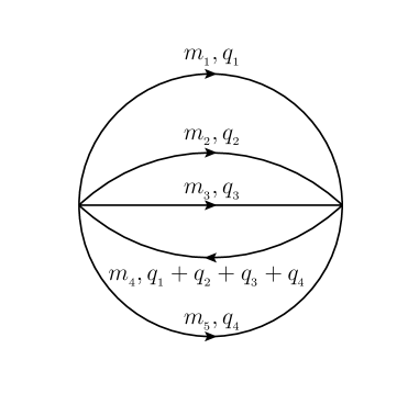
Figure 1: Four-loop vacuum diagram with five propagators.

The expression of 4-loop vacuum integral with five propagates in Fig. 1 can be written as

$$U_{{}_{5}}=\Big{(}\Lambda_{{}_{\rm RE}}^{2}\Big{)}^{8-2D}\int{d^{D}{\bf q}\over(2\pi)^{D}}{1\over(q_{{}_{1}}^{2}-m_{{}_{1}}^{2})(q_{{}_{2}}^{2}-m_{{}_{2}}^{2})(q_{{}_{3}}^{2}-m_{{}_{3}}^{2})}$$

$$\hskip 31.2982pt\times{1\over[(q_{{}_{1}}+q_{{}_{2}}+q_{{}_{3}}+q_{{}_{4}})^{2}-m_{{}_{4}}^{2}](q_{{}_{4}}^{2}-m_{{}_{5}}^{2})}\>,$$ (1)

where $\Lambda_{{}_{\rm RE}}$ denotes the renormalization energy scale and $D=4-2\varepsilon$ is the number of dimensions in dimensional regularization, ${\bf q}=(q_{{}_{1}},\;\cdots,\;q_{{}_{4}})$, ${d^{D}{\bf q}\over(2\pi)^{D}}={d^{D}q_{{}_{1}}\over(2\pi)^{D}}{d^{D}q_{{}_{2}}\over(2\pi)^{D}}{d^{D}q_{{}_{3}}\over(2\pi)^{D}}{d^{D}q_{{}_{4}}\over(2\pi)^{D}}$. The Feynman integral is hard to calculate analytically, if all virtual masses are nonzero. So, one can extract the virtual masses from the integral, to facilitate further calculation. Adopting the notation of Refs. Feng2018 ; Feng2019 , the four-loop vacuum integral with five propagates is written as

$$U_{{}_{5}}=\frac{\Big{(}\Lambda_{{}_{\rm RE}}^{2}\Big{)}^{8-2D}}{(2\pi i)^{4}}\int_{-i\infty}^{+i\infty}d{\bf s}\Big{[}\prod\limits_{i=1}^{4}(-m_{{}_{i}}^{2})^{s_{{}_{i}}}\Gamma(-s_{{}_{i}})\Gamma(1+s_{{}_{i}})\Big{]}I_{q}\>,$$ (2)

where ${\bf s}=(s_{{}_{1}},\;\cdots,\;s_{{}_{4}})$, $d{\bf s}=ds_{{}_{1}}ds_{{}_{2}}ds_{{}_{3}}ds_{{}_{4}}$ and

$$I_{q}\equiv\int{d^{D}{\bf q}\over(2\pi)^{D}}{1\over(q_{{}_{1}}^{2})^{1+s_{{}_{1}}}(q_{{}_{2}}^{2})^{1+s_{{}_{2}}}(q_{{}_{3}}^{2})^{1+s_{{}_{3}}}[(q_{{}_{1}}+q_{{}_{2}}+q_{{}_{3}}+q_{{}_{4}})^{2}]^{1+s_{{}_{4}}}(q_{{}_{4}}^{2}-m_{{}_{5}}^{2})}\>.$$ (3)

The integral $I_{q}$ just keeps one mass $m_{{}_{5}}$, which can be easily calculated analytically.

And then, the Mellin-Barnes representation of the four-loop vacuum integral in Eq. (2) is written as

$$U_{{}_{5}}={-m_{{}_{5}}^{6}\over(2\pi i)^{4}(4\pi)^{8}}\Big{(}{4\pi\Lambda_{{}_{\rm RE}}^{2}\over m_{{}_{5}}^{2}}\Big{)}^{8-2D}\int_{-i\infty}^{+i\infty}d{\bf s}\Big{[}\prod\limits_{i=1}^{4}\Big{(}{m_{{}_{i}}^{2}\over m_{{}_{5}}^{2}}\Big{)}^{s_{{}_{i}}}\Gamma(-s_{{}_{i}})\Big{]}$$

$$\hskip 28.45274pt\times\Big{[}\prod\limits_{i=1}^{4}\Gamma({D\over 2}-1-s_{{}_{i}})\Big{]}\Gamma(4-{3D\over 2}+\sum\limits_{i=1}^{4}s_{{}_{i}})\Gamma(5-2D+\sum\limits_{i=1}^{4}s_{{}_{i}})\;.$$ (4)

It is well known that zero and negative integers are simple poles of the function $\Gamma(z)$. As all $s_{{}_{i}}$ contours are closed to the right in complex planes, one can find that the analytic expression of the integral can be written as the linear combination of generalized hypergeometric functions. Taking the residue of the pole of $\Gamma(-s_{{}_{i}}),\;(i=1,\cdots,\;4)$, we derive one linear independent term of the integral:

$$U_{{}_{5}}\ni{-m_{{}_{5}}^{6}\over(4\pi)^{8}}\Big{(}{4\pi\Lambda_{{}_{\rm RE}}^{2}\over m_{{}_{5}}^{2}}\Big{)}^{8-2D}\sum\limits_{n_{{}_{1}}=0}^{\infty}\sum_{n_{{}_{2}}=0}^{\infty}\sum_{n_{{}_{3}}=0}^{\infty}\sum_{n_{{}_{4}}=0}^{\infty}(-)^{\sum\limits_{i=1}^{4}n_{{}_{i}}}x_{{}_{1}}^{n_{{}_{1}}}x_{{}_{2}}^{n_{{}_{2}}}x_{{}_{3}}^{n_{{}_{3}}}x_{{}_{4}}^{n_{{}_{4}}}$$

$$\hskip 28.45274pt\times\Big{[}\prod\limits_{i=1}^{4}\Gamma({D\over 2}-1-n_{{}_{i}})(n_{{}_{i}}!)^{-1}\Big{]}\Gamma(4-{3D\over 2}+\sum\limits_{i=1}^{4}n_{{}_{i}})\Gamma(5-2D+\sum\limits_{i=1}^{4}n_{{}_{i}})\>,$$ (5)

with $x_{{}_{i}}={m_{{}_{i}}^{2}\over m_{{}_{5}}^{2}},\;(i=1,\cdots,\;4)$.

We adopt the well-known identity

$$\Gamma(z-n)\Gamma(1-z+n)=(-)^{n}\Gamma(z)\Gamma(1-z)=(-)^{n}\pi/\sin\pi z\>.$$ (6)

Then, Eq. (5) is written as

$$U_{{}_{5}}\ni{-m_{{}_{5}}^{6}\over(4\pi)^{8}}\Big{(}{4\pi\Lambda_{{}_{\rm RE}}^{2}\over m_{{}_{5}}^{2}}\Big{)}^{8-2D}{\pi^{4}\over\sin^{4}\frac{\pi D}{2}}T_{{}_{5}}({\bf a},\;{\bf b}\;\Big{|}\;{\bf x})\;,$$ (7)

with

$$T_{{}_{5}}({\bf a},\;{\bf b}\;\Big{|}\;{\bf x})=\sum\limits_{n_{{}_{1}}=0}^{\infty}\sum_{n_{{}_{2}}=0}^{\infty}\sum_{n_{{}_{3}}=0}^{\infty}\sum_{n_{{}_{4}}=0}^{\infty}A_{{}_{n_{{}_{1}}n_{{}_{2}}n_{{}_{3}}n_{{}_{4}}}}x_{{}_{1}}^{n_{{}_{1}}}x_{{}_{2}}^{n_{{}_{2}}}x_{{}_{3}}^{n_{{}_{3}}}x_{{}_{4}}^{n_{{}_{4}}}\>,$$ (8)

where ${\bf x}=(x_{{}_{1}},x_{{}_{2}},x_{{}_{3}},x_{{}_{4}})$, ${\bf a}=(a_{{}_{1}},a_{{}_{2}})$ and ${\bf b}=(b_{{}_{1}},b_{{}_{2}},b_{{}_{3}},b_{{}_{4}})$ with

$$a_{{}_{1}}=4-{3D\over 2},\;\;a_{{}_{2}}=5-2D,\;\;b_{{}_{1}}=b_{{}_{2}}=b_{{}_{3}}=b_{{}_{4}}=2-{D\over 2}\>,$$ (9)

and the coefficient $A_{{}_{n_{{}_{1}}n_{{}_{2}}n_{{}_{3}}n_{{}_{4}}}}$ is

$$A_{{}_{n_{{}_{1}}n_{{}_{2}}n_{{}_{3}}n_{{}_{4}}}}={\Gamma(a_{{}_{1}}+\sum\limits_{i=1}^{4}n_{{}_{i}})\Gamma(a_{{}_{2}}+\sum\limits_{i=1}^{4}n_{{}_{i}})\over\prod\limits_{i=1}^{4}n_{{}_{i}}!\Gamma(b_{{}_{i}}+n_{{}_{i}})}\>.$$ (10)

Here, we just derive one linear independent term of the integral. We still need to derive other linear independent terms of the integral.

We define the auxiliary function

$$\Phi_{{}_{5}}({\bf a},\;{\bf b}\;\Big{|}\;{\bf x},\;{\bf u},\;{\bf v})={\bf u}^{\bf a}{\bf v}^{{\bf b}-{\bf e}_{{}_{4}}}T_{{}_{5}}({\bf a},\;{\bf b}\;\Big{|}\;{\bf x})\;,$$ (11)

with the intermediate variables ${\bf u}=(u_{{}_{1}},\;u_{{}_{2}})=(1,\;1)$, ${\bf v}=(v_{{}_{1}},\;v_{{}_{2}},\;v_{{}_{3}},\;v_{{}_{4}})=(1,\;1,\;1,\;1)$, ${\bf e}_{{}_{4}}=(1,\;1,\;1,\;1)$. Through Miller’s transformation Miller68 ; Miller72 , one can obtain

$$\vartheta_{{}_{u_{j}}}\Phi_{{}_{5}}({\bf a},\;{\bf b}\;\Big{|}\;{\bf x},\;{\bf u},\;{\bf v})=a_{{}_{j}}\Phi_{{}_{5}}({\bf a},\;{\bf b}\;\Big{|}\;{\bf x},\;{\bf u},\;{\bf v})\;,\;(j=1,2)\>,$$

$$\vartheta_{{}_{v_{k}}}\Phi_{{}_{5}}({\bf a},\;{\bf b}\;\Big{|}\;{\bf x},\;{\bf u},\;{\bf v})=(b_{{}_{k}}-1)\Phi_{{}_{5}}({\bf a},\;{\bf b}\;\Big{|}\;{\bf x},\;{\bf u},\;{\bf v})\;,\;(k=1,\cdots,4)\>,$$ (12)

which naturally induces the notion of GKZ hypergeometric system. $\vartheta_{{}_{x_{{}_{k}}}}=x_{{}_{k}}\partial_{{}_{x_{{}_{k}}}}$ denotes the Euler operators, and $\partial_{{}_{x_{{}_{k}}}}=\partial/\partial x_{{}_{k}}$.

Through the transformation

$$z_{{}_{j}}={1\over u_{{}_{j}}},\;(j=1,2),\;\;z_{{}_{2+k}}=v_{{}_{k}},\;z_{{}_{6+k}}={x_{{}_{k}}\over u_{{}_{1}}u_{{}_{2}}v_{{}_{k}}},\;(k=1,\cdots,4),$$ (13)

we can finally have the GKZ hypergeometric system for the four-loop vacuum integral with five propagates:

$$\mathbf{A_{{}_{5}}}\cdot\vec{\vartheta}_{{}_{5}}\Phi_{{}_{5}}=\mathbf{B_{{}_{5}}}\Phi_{{}_{5}}\;,$$ (14)

where

$$\mathbf{A_{{}_{5}}}=\left(\begin{array}[]{cccccccccc}1&0&0&0&0&0&1&1&1&1\\ 0&1&0&0&0&0&1&1&1&1\\ 0&0&1&0&0&0&-1&0&0&0\\ 0&0&0&1&0&0&0&-1&0&0\\ 0&0&0&0&1&0&0&0&-1&0\\ 0&0&0&0&0&1&0&0&0&-1\\ \end{array}\right)\;,$$ (21)

$$\vec{\vartheta}_{{}_{5}}^{\;T}=(\vartheta_{{}_{z_{{}_{1}}}},\;\cdots,\;\vartheta_{{}_{z_{{}_{10}}}})\;,$$

$$\mathbf{B_{{}_{5}}}^{T}=(-a_{{}_{1}},\;-a_{{}_{2}},\;b_{{}_{1}}-1,\;b_{{}_{2}}-1,\;b_{{}_{3}}-1,\;b_{{}_{4}}-1)\;.$$ (22)

Correspondingly, the dual matrix $\mathbf{\tilde{A}_{{}_{5}}}$ of $\mathbf{A_{{}_{5}}}$ is

$$\mathbf{\tilde{A}_{{}_{5}}}=\left(\begin{array}[]{cccccccccc}-1&-1&1&0&0&0&1&0&0&0\\ -1&-1&0&1&0&0&0&1&0&0\\ -1&-1&0&0&1&0&0&0&1&0\\ -1&-1&0&0&0&1&0&0&0&1\end{array}\right).$$ (27)

The row vectors of the matrix $\mathbf{\tilde{A}_{{}_{5}}}$ induce the integer sublattice $\mathbf{B}$ which can be used to construct the formal solutions in hypergeometric series.

Defining the combined variables

$$y_{{}_{1}}={z_{{}_{3}}z_{{}_{7}}\over z_{{}_{1}}z_{{}_{2}}}\;,\quad y_{{}_{2}}={z_{{}_{4}}z_{{}_{8}}\over z_{{}_{1}}z_{{}_{2}}}\;,\quad y_{{}_{3}}={z_{{}_{5}}z_{{}_{9}}\over z_{{}_{1}}z_{{}_{2}}}\;,\quad y_{{}_{4}}={z_{{}_{6}}z_{{}_{10}}\over z_{{}_{1}}z_{{}_{2}}}\;,$$ (28)

we can write the solutions satisfying Eq. (14) as

$$\Phi_{{}_{5}}({\mathbf{z}})=\Big{(}\prod\limits_{i=1}^{10}z_{{}_{i}}^{\alpha_{{}_{i}}}\Big{)}\varphi_{{}_{5}}(y_{{}_{1}},\;y_{{}_{2}},\;y_{{}_{3}},\;y_{{}_{4}})\;.$$ (29)

Here $\vec{\alpha}^{\>T}=(\alpha_{{}_{1}},\;\cdots,\;\alpha_{{}_{10}})$ denotes a sequence of complex number such that

$$\mathbf{A_{{}_{5}}}\cdot\vec{\alpha}=\mathbf{B_{{}_{5}}}\;.$$ (30)

In the following Sec. V, we will show the analytical hypergeometric series solutions solving from the GKZ hypergeometric system in Eq. (14).

III GKZ hypergeometric system of 4-loop vacuum integrals with six propagates

III.1 4-loop vacuum diagram with six propagates for type A

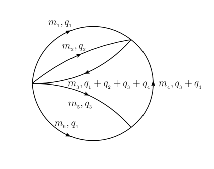
Figure 2: Four-loop vacuum diagram with six propagators for type A.

The four-loop vacuum diagrams with six propagates have two topologies, which one can be seen in Fig. 2. The expression of the four-loop vacuum integral with six propagates for type A in Fig. 2 can be written as

$$U_{{}_{6A}}=\Big{(}\Lambda_{{}_{\rm RE}}^{2}\Big{)}^{8-2D}\int{d^{D}{\bf q}\over(2\pi)^{D}}{1\over(q_{{}_{1}}^{2}-m_{{}_{1}}^{2})(q_{{}_{2}}^{2}-m_{{}_{2}}^{2})[(q_{{}_{1}}+q_{{}_{2}}+q_{{}_{3}}+q_{{}_{4}})^{2}-m_{{}_{3}}^{2}]}$$

$$\hskip 31.2982pt\times{1\over[(q_{{}_{3}}+q_{{}_{4}})^{2}-m_{{}_{4}}^{2}](q_{{}_{3}}^{2}-m_{{}_{5}}^{2})(q_{{}_{4}}^{2}-m_{{}_{6}}^{2})}.$$ (31)

Similarly, we can derive one linear independent term of the integral:

$$U_{{}_{6A}}\ni{m_{{}_{6}}^{4}\over(4\pi)^{8}}\Big{(}{4\pi\Lambda_{{}_{\rm RE}}^{2}\over m_{{}_{6}}^{2}}\Big{)}^{8-2D}{\pi^{4}\over\sin^{4}\frac{\pi D}{2}}T_{{}_{6A}}({\bf a},\;{\bf b}\;\Big{|}\;{\bf x})\;,$$ (32)

with

$$T_{{}_{6A}}({\bf a},\;{\bf b}\;\Big{|}\;{\bf x})={\bf{\sum\limits_{{n}=0}^{\infty}}}A_{{}_{\bf n}}{\bf x^{n}},$$ (33)

where ${\bf n}=(n_{{}_{1}},\;\cdots,\;n_{{}_{5}})$, ${\bf x}=(x_{{}_{1}},\;\cdots,\;x_{{}_{5}})$, $x_{{}_{i}}={m_{{}_{i}}^{2}\over m_{{}_{6}}^{2}},\;(i=1,\cdots,5)$, ${\bf a}=(a_{{}_{1}},\;\cdots,a_{{}_{5}})$ and ${\bf b}=(b_{{}_{1}},\;\cdots,b_{{}_{6}})$ with

$$a_{{}_{1}}=5-{3D\over 2},\;a_{{}_{2}}=6-2D,\;a_{{}_{3}}=3-D,\;a_{{}_{4}}=4-{3D\over 2},\;a_{{}_{5}}=1,$$

$$b_{{}_{1}}=b_{{}_{2}}=b_{{}_{3}}=b_{{}_{4}}=2-{D\over 2},\;b_{{}_{5}}=4-D,\;b_{{}_{6}}=5-{3D\over 2}\>,$$ (34)

and the coefficient $A_{{}_{\bf n}}$ is

$$A_{{}_{{\bf n}}}={\Gamma(a_{{}_{1}}+\sum\limits_{i=1}^{5}n_{{}_{i}})\Gamma(a_{{}_{2}}+\sum\limits_{i=1}^{5}n_{{}_{i}})\Gamma(a_{{}_{3}}+\sum\limits_{i=1}^{3}n_{{}_{i}})\Gamma(a_{{}_{4}}+\sum\limits_{i=1}^{3}n_{{}_{i}})\Gamma(a_{{}_{5}}+n_{{}_{4}})\over\Big{[}\prod\limits_{i=1}^{5}n_{{}_{i}}!\Big{]}\Big{[}\prod\limits_{i=1}^{3}\Gamma(b_{{}_{i}}+n_{{}_{i}})\Big{]}\Gamma(b_{{}_{4}}+n_{{}_{5}})\Gamma(b_{{}_{5}}+\sum\limits_{i=1}^{4}n_{{}_{i}})\Gamma(b_{{}_{6}}+\sum\limits_{i=1}^{4}n_{{}_{i}})}.$$ (35)

We also define the auxiliary function

$$\Phi_{{}_{6A}}({\bf a},\;{\bf b}\;\Big{|}\;{\bf x},\;{\bf u},\;{\bf v})={\bf u}^{\bf a}{\bf v}^{{\bf b}-{\bf e}_{{}_{6}}}T_{{}_{6A}}({\bf a},\;{\bf b}\;\Big{|}\;{\bf x})\;,$$ (36)

with the intermediate variables ${\bf u}=(u_{{}_{1}},\cdots,u_{{}_{5}})=(1,\;1,\;1,\;1,\;1)$, ${\bf v}=(v_{{}_{1}},\cdots,v_{{}_{6}})$, ${\bf v}={\bf e}_{{}_{6}}=(1,\;1,\;1,\;1,\;1,\;1)$. One can derive the GKZ hypergeometric system for the four-loop vacuum integral with six propagates for type A:

$$\mathbf{A_{{}_{6A}}}\cdot\vec{\vartheta}_{{}_{6A}}\Phi_{{}_{6A}}=\mathbf{B_{{}_{6A}}}\Phi_{{}_{6A}}\;,$$ (37)

where

$$\mathbf{A_{{}_{6A}}}=\left(\begin{array}[]{cc}\mathbf{I_{{}_{11\times 11}}}&\mathbf{A_{{}_{X6A}}}\\ \end{array}\right)\;,$$ (39)

$$\mathbf{A_{{}_{X6A}}}^{\;T}=\left(\begin{array}[]{ccccccccccc}1&1&1&1&0&-1&0&0&0&-1&-1\\ 1&1&1&1&0&0&-1&0&0&-1&-1\\ 1&1&1&1&0&0&0&-1&0&-1&-1\\ 1&1&0&0&1&0&0&0&0&-1&-1\\ 1&1&0&0&0&0&0&0&-1&0&0\\ \end{array}\right)\;,$$ (45)

$$\vec{\vartheta}_{{}_{6A}}^{\;T}=(\vartheta_{{}_{z_{{}_{1}}}},\cdots,\;\vartheta_{{}_{z_{{}_{16}}}})\;,$$

$$\mathbf{B_{{}_{6A}}}^{\;T}=(-a_{{}_{1}},\;\cdots,\;-a_{{}_{5}},\;b_{{}_{1}}-1,\;\cdots,\;b_{{}_{6}}-1)\;.$$ (46)

Here, $\mathbf{I_{{}_{11\times 11}}}$ is an ${11\times 11}$ unit matrix.

Correspondingly the dual matrix $\mathbf{\tilde{A}_{{}_{6A}}}$ of $\mathbf{A_{{}_{6A}}}$ is

$$\mathbf{\tilde{A}_{{}_{6A}}}=\left(\begin{array}[]{cc}-\mathbf{A_{{}_{X6A}}}^{\;T}&\mathbf{I_{{}_{5\times 5}}}\\ \end{array}\right).$$ (48)

Here, $\mathbf{I_{{}_{5\times 5}}}$ is a ${5\times 5}$ unit matrix.

III.2 4-loop vacuum diagram with six propagates for type B

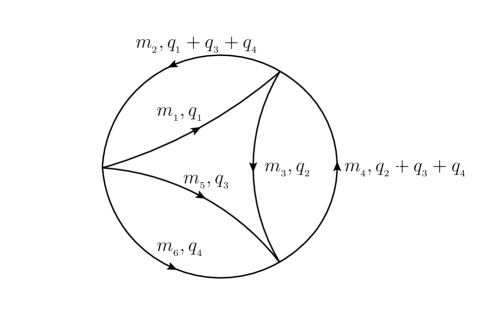
Figure 3: Four-loop vacuum diagram with six propagators for type B.

The expression of the four-loop vacuum integral with six propagates for type B in Fig. 3 can be written as

$$U_{{}_{6B}}=\Big{(}\Lambda_{{}_{\rm RE}}^{2}\Big{)}^{8-2D}\int{d^{D}{\bf q}\over(2\pi)^{D}}{1\over(q_{{}_{1}}^{2}-m_{{}_{1}}^{2})[(q_{{}_{1}}+q_{{}_{3}}+q_{{}_{4}})^{2}-m_{{}_{2}}^{2}]}$$

$$\hskip 31.2982pt\times{1\over(q_{{}_{2}}^{2}-m_{{}_{3}}^{2})[(q_{{}_{2}}+q_{{}_{3}}+q_{{}_{4}})^{2}-m_{{}_{4}}^{2}](q_{{}_{3}}^{2}-m_{{}_{5}}^{2})(q_{{}_{4}}^{2}-m_{{}_{6}}^{2})}.$$ (49)

We can derive one linear independent term of the integral:

$$U_{{}_{6B}}\ni{m_{{}_{6}}^{4}\over(4\pi)^{8}}\Big{(}{4\pi\Lambda_{{}_{\rm RE}}^{2}\over m_{{}_{6}}^{2}}\Big{)}^{8-2D}{\pi^{4}\sin^{2}\pi D\over\sin^{5}\frac{\pi D}{2}\sin\frac{3\pi D}{2}}T_{{}_{6B}}({\bf a},\;{\bf b}\;\Big{|}\;{\bf x})\;,$$ (50)

with

$$T_{{}_{6B}}({\bf a},\;{\bf b}\;\Big{|}\;{\bf x})={\bf{\sum\limits_{{n}=0}^{\infty}}}A_{{}_{\bf n}}{\bf x^{n}},$$ (51)

where ${\bf n}=(n_{{}_{1}},\;\cdots,\;n_{{}_{5}})$, ${\bf x}=(x_{{}_{1}},\;\cdots,\;x_{{}_{5}})$, $x_{{}_{i}}={m_{{}_{i}}^{2}\over m_{{}_{6}}^{2}}$, ${\bf a}=(a_{{}_{1}},\;\cdots,a_{{}_{6}})$ and ${\bf b}=(b_{{}_{1}},\;\cdots,b_{{}_{7}})$ with

$$a_{{}_{1}}=5-{3D\over 2},\;a_{{}_{2}}=6-2D,\;a_{{}_{3}}=a_{{}_{5}}=2-{D\over 2},\;a_{{}_{4}}=a_{{}_{6}}=3-D\;,$$

$$b_{{}_{1}}=b_{{}_{2}}=b_{{}_{3}}=b_{{}_{4}}=b_{{}_{5}}=2-{D\over 2},\;b_{{}_{6}}=4-D,\;b_{{}_{7}}=5-{3D\over 2}\>,$$ (52)

and the coefficient $A_{{}_{\bf n}}$ is

$$A_{{}_{{\bf n}}}={\Gamma(a_{{}_{1}}+\sum\limits_{i=1}^{5}n_{{}_{i}})\Gamma(a_{{}_{2}}+\sum\limits_{i=1}^{5}n_{{}_{i}})\Gamma(a_{{}_{3}}+\sum\limits_{i=1}^{2}n_{{}_{i}})\Gamma(a_{{}_{4}}+\sum\limits_{i=1}^{2}n_{{}_{i}})\Gamma(a_{{}_{5}}+\sum\limits_{i=3}^{4}n_{{}_{i}})\Gamma(a_{{}_{6}}+\sum\limits_{i=3}^{4}n_{{}_{i}})\over\Big{[}\prod\limits_{i=1}^{5}n_{{}_{i}}!\Gamma(b_{{}_{i}}+n_{{}_{i}})\Big{]}\Gamma(b_{{}_{6}}+\sum\limits_{i=1}^{4}n_{{}_{i}})\Gamma(b_{{}_{7}}+\sum\limits_{i=1}^{4}n_{{}_{i}})}.$$ (53)

We can define the auxiliary function

$$\Phi_{{}_{6B}}({\bf a},\;{\bf b}\;\Big{|}\;{\bf x},\;{\bf u},\;{\bf v})={\bf u}^{\bf a}{\bf v}^{{\bf b}-{\bf e}_{{}_{7}}}T_{{}_{6B}}({\bf a},\;{\bf b}\;\Big{|}\;{\bf x})\;,$$ (54)

with the intermediate variables ${\bf u}=(u_{{}_{1}},\cdots,u_{{}_{6}})=(1,\;1,\;1,\;1,\;1,\;1)$, ${\bf v}=(v_{{}_{1}},\cdots,v_{{}_{7}})$, ${\bf v}={\bf e}_{{}_{7}}=(1,\;1,\;1,\;1,\;1,\;1,\;1)$. One can derive the GKZ hypergeometric system for the four-loop vacuum integral with six propagates for type B:

$$\mathbf{A_{{}_{6B}}}\cdot\vec{\vartheta}_{{}_{6B}}\Phi_{{}_{6B}}=\mathbf{B_{{}_{6B}}}\Phi_{{}_{6B}}\;,$$ (55)

where

$$\mathbf{A_{{}_{6B}}}=\left(\begin{array}[]{cc}\mathbf{I_{{}_{13\times 13}}}&\mathbf{A_{{}_{X6B}}}\\ \end{array}\right)\;,$$ (57)

$$\mathbf{A_{{}_{X6B}}}^{\;T}=\left(\begin{array}[]{ccccccccccccc}1&1&1&1&0&0&-1&0&0&0&0&-1&-1\\ 1&1&1&1&0&0&0&-1&0&0&0&-1&-1\\ 1&1&0&0&1&1&0&0&-1&0&0&-1&-1\\ 1&1&0&0&1&1&0&0&0&-1&0&-1&-1\\ 1&1&0&0&0&0&0&0&0&0&-1&0&0\\ \end{array}\right)\;,$$ (63)

$${\vec{\vartheta}_{{}_{6B}}}^{\;T}=(\vartheta_{{}_{z_{{}_{1}}}},\cdots,\;\vartheta_{{}_{z_{{}_{18}}}})\;,$$

$$\mathbf{B_{{}_{6B}}}^{\;T}=(-a_{{}_{1}},\;\cdots,\;-a_{{}_{6}},\;b_{{}_{1}}-1,\;\cdots,\;b_{{}_{7}}-1)\;.$$ (64)

Here, $\mathbf{I_{{}_{13\times 13}}}$ is a ${13\times 13}$ unit matrix.

IV GKZ hypergeometric system of 4-loop vacuum integrals with seven propagates

IV.1 4-loop vacuum diagram with seven propagates for type A

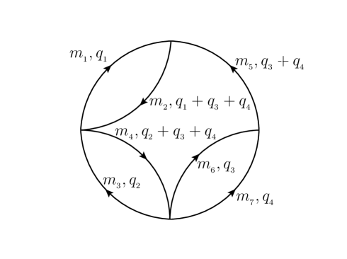
Figure 4: Four-loop vacuum diagram with seven propagators for type A.

The expression of the four-loop vacuum integral with seven propagates for type A in Fig. 4 can be written as

$$U_{{}_{7A}}=\Big{(}\Lambda_{{}_{\rm RE}}^{2}\Big{)}^{8-2D}\int{d^{D}{\bf q}\over(2\pi)^{D}}{1\over(q_{{}_{1}}^{2}-m_{{}_{1}}^{2})[(q_{{}_{1}}+q_{{}_{3}}+q_{{}_{4}})^{2}-m_{{}_{2}}^{2}](q_{{}_{2}}^{2}-m_{{}_{3}}^{2})}$$

$$\hskip 31.2982pt\times{1\over[(q_{{}_{2}}+q_{{}_{3}}+q_{{}_{4}})^{2}-m_{{}_{4}}^{2}][(q_{{}_{3}}+q_{{}_{4}})^{2}-m_{{}_{5}}^{2}](q_{{}_{3}}^{2}-m_{{}_{6}}^{2})(q_{{}_{4}}^{2}-m_{{}_{7}}^{2})}.$$ (65)

We can derive one linear independent term of the integral:

$$U_{{}_{7A}}\ni{-m_{{}_{7}}^{2}\over(4\pi)^{8}}\Big{(}{4\pi\Lambda_{{}_{\rm RE}}^{2}\over m_{{}_{7}}^{2}}\Big{)}^{8-2D}{\pi^{4}\sin^{2}\pi D\over\sin^{5}\frac{\pi D}{2}\sin\frac{3\pi D}{2}}T_{{}_{7A}}({\bf a},\;{\bf b}\;\Big{|}\;{\bf x})\;,$$ (66)

with

$$T_{{}_{7A}}({\bf a},\;{\bf b}\;\Big{|}\;{\bf x})={\bf{\sum\limits_{{n}=0}^{\infty}}}A_{{}_{\bf n}}{\bf x^{n}},$$ (67)

where ${\bf n}=(n_{{}_{1}},\;\cdots,\;n_{{}_{6}})$, ${\bf x}=(x_{{}_{1}},\;\cdots,\;x_{{}_{6}})$, $x_{{}_{i}}={m_{{}_{i}}^{2}\over m_{{}_{7}}^{2}}$, ${\bf a}=(a_{{}_{1}},\;\cdots,a_{{}_{7}})$ and ${\bf b}=(b_{{}_{1}},\;\cdots,b_{{}_{7}})$ with

$$a_{{}_{1}}=6-{3D\over 2},\;a_{{}_{2}}=7-2D,\;a_{{}_{3}}=a_{{}_{5}}=2-{D\over 2},\;a_{{}_{4}}=a_{{}_{6}}=3-D,\;a_{{}_{7}}=1\;,$$

$$b_{{}_{1}}=b_{{}_{2}}=b_{{}_{3}}=b_{{}_{4}}=b_{{}_{5}}=2-{D\over 2},\;b_{{}_{6}}=5-D,\;b_{{}_{7}}=6-{3D\over 2}\>,$$ (68)

and the coefficient $A_{{}_{\bf n}}$ is

$$A_{{}_{{\bf n}}}=\Gamma(a_{{}_{1}}+\sum\limits_{i=1}^{6}n_{{}_{i}})\Gamma(a_{{}_{2}}+\sum\limits_{i=1}^{6}n_{{}_{i}})\Gamma(a_{{}_{3}}+\sum\limits_{i=1}^{2}n_{{}_{i}})$$

$$\hskip 28.45274pt\times{\Gamma(a_{{}_{4}}+\sum\limits_{i=1}^{2}n_{{}_{i}})\Gamma(a_{{}_{5}}+\sum\limits_{i=3}^{4}n_{{}_{i}})\Gamma(a_{{}_{6}}+\sum\limits_{i=3}^{4}n_{{}_{i}})\Gamma(a_{{}_{7}}+n_{{}_{5}})\over\Big{[}\prod\limits_{i=1}^{6}n_{{}_{i}}!\Big{]}\Big{[}\prod\limits_{i=1}^{4}\Gamma(b_{{}_{i}}+n_{{}_{i}})\Big{]}\Gamma(b_{{}_{5}}+n_{{}_{6}})\Gamma(b_{{}_{6}}+\sum\limits_{i=1}^{5}n_{{}_{i}})\Gamma(b_{{}_{7}}+\sum\limits_{i=1}^{5}n_{{}_{i}})}.$$ (69)

We define the auxiliary function

$$\Phi_{{}_{7A}}({\bf a},\;{\bf b}\;\Big{|}\;{\bf x},\;{\bf u},\;{\bf v})={\bf u}^{\bf a}{\bf v}^{{\bf b}-{\bf e}_{{}_{7}}}T_{{}_{7A}}({\bf a},\;{\bf b}\;\Big{|}\;{\bf x})\;,$$ (70)

with the intermediate variables ${\bf u}=(u_{{}_{1}},\cdots,u_{{}_{7}})$, ${\bf v}=(v_{{}_{1}},\cdots,v_{{}_{7}})$, ${\bf u}={\bf v}={\bf e}_{{}_{7}}=(1,\;1,\;1,\;1,\;1,\;1,\;1)$. One can derive the GKZ hypergeometric system for the four-loop vacuum integral with seven propagates for type A:

$$\mathbf{A_{{}_{7A}}}\cdot\vec{\vartheta}_{{}_{7A}}\Phi_{{}_{7A}}=\mathbf{B_{{}_{7A}}}\Phi_{{}_{7A}}\;,$$ (71)

where

$$\mathbf{A_{{}_{7A}}}=\left(\begin{array}[]{cc}\mathbf{I_{{}_{14\times 14}}}&\mathbf{A_{{}_{X7A}}}\\ \end{array}\right)\;,$$ (73)

$$\mathbf{A_{{}_{X7A}}}^{\;T}=\left(\begin{array}[]{cccccccccccccc}1&1&1&1&0&0&0&-1&0&0&0&0&-1&-1\\ 1&1&1&1&0&0&0&0&-1&0&0&0&-1&-1\\ 1&1&0&0&1&1&0&0&0&-1&0&0&-1&-1\\ 1&1&0&0&1&1&0&0&0&0&-1&0&-1&-1\\ 1&1&0&0&0&0&1&0&0&0&0&0&-1&-1\\ 1&1&0&0&0&0&0&0&0&0&0&-1&0&0\\ \end{array}\right)\;,$$ (80)

$${\vec{\vartheta}_{{}_{7A}}}^{\;T}=(\vartheta_{{}_{z_{{}_{1}}}},\cdots,\;\vartheta_{{}_{z_{{}_{20}}}})\;,$$

$$\mathbf{B_{{}_{7A}}}^{\;T}=(-a_{{}_{1}},\;\cdots,\;-a_{{}_{7}},\;b_{{}_{1}}-1,\;\cdots,\;b_{{}_{7}}-1)\;.$$ (81)

Here, $\mathbf{I_{{}_{14\times 14}}}$ is a ${14\times 14}$ unit matrix.

Correspondingly the dual matrix $\mathbf{\tilde{A}_{{}_{7A}}}$ of $\mathbf{A_{{}_{7A}}}$ is

$$\mathbf{\tilde{A}_{{}_{7A}}}=\left(\begin{array}[]{cc}-\mathbf{A_{{}_{X7A}}}^{\;T}&\mathbf{I_{{}_{6\times 6}}}\\ \end{array}\right),$$ (83)

where $\mathbf{I_{{}_{6\times 6}}}$ is a ${6\times 6}$ unit matrix.

IV.2 4-loop vacuum diagram with seven propagates for type B

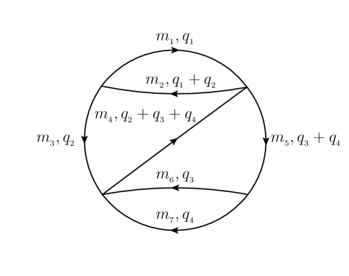
Figure 5: Four-loop vacuum diagram with seven propagators for type B.

The expression of the four-loop vacuum integral with seven propagates for type B in Fig. 5 is

$$U_{{}_{7B}}=\Big{(}\Lambda_{{}_{\rm RE}}^{2}\Big{)}^{8-2D}\int{d^{D}{\bf q}\over(2\pi)^{D}}{1\over(q_{{}_{1}}^{2}-m_{{}_{1}}^{2})[(q_{{}_{1}}+q_{{}_{2}})^{2}-m_{{}_{2}}^{2}](q_{{}_{2}}^{2}-m_{{}_{3}}^{2})}$$

$$\hskip 31.2982pt\times{1\over[(q_{{}_{2}}+q_{{}_{3}}+q_{{}_{4}})^{2}-m_{{}_{4}}^{2}][(q_{{}_{3}}+q_{{}_{4}})^{2}-m_{{}_{5}}^{2}](q_{{}_{3}}^{2}-m_{{}_{6}}^{2})(q_{{}_{4}}^{2}-m_{{}_{7}}^{2})}.$$ (84)

We can derive one linear independent term of the integral:

$$U_{{}_{7B}}\ni{m_{{}_{7}}^{2}\over(4\pi)^{8}}\Big{(}{4\pi\Lambda_{{}_{\rm RE}}^{2}\over m_{{}_{7}}^{2}}\Big{)}^{8-2D}{\pi^{4}\over\sin^{4}\frac{\pi D}{2}}T_{{}_{7B}}({\bf a},\;{\bf b}\;\Big{|}\;{\bf x})\;,$$ (85)

with

$$T_{{}_{7B}}({\bf a},\;{\bf b}\;\Big{|}\;{\bf x})={\bf{\sum\limits_{{n}=0}^{\infty}}}A_{{}_{\bf n}}{\bf x^{n}},$$ (86)

where ${\bf n}=(n_{{}_{1}},\;\cdots,\;n_{{}_{6}})$, ${\bf x}=(x_{{}_{1}},\;\cdots,\;x_{{}_{6}})$, $x_{{}_{i}}={m_{{}_{i}}^{2}\over m_{{}_{7}}^{2}}$, ${\bf a}=(a_{{}_{1}},\;\cdots,a_{{}_{8}})$ and ${\bf b}=(b_{{}_{1}},\;\cdots,b_{{}_{8}})$ with

$$a_{{}_{1}}=6-{3D\over 2},\;a_{{}_{2}}=7-2D,\;a_{{}_{3}}=5-{3D\over 2},\;a_{{}_{4}}=4-D,\;$$

$$a_{{}_{5}}=2-{D\over 2},\;a_{{}_{6}}=3-D,\;a_{{}_{7}}=a_{{}_{8}}=1,\;b_{{}_{1}}=b_{{}_{2}}=b_{{}_{3}}=b_{{}_{4}}=2-{D\over 2},\;$$

$$b_{{}_{5}}=3-{D\over 2},\;b_{{}_{6}}=4-D,\;b_{{}_{7}}=5-D,\;b_{{}_{8}}=6-{3D\over 2}\>,$$ (87)

and the coefficient $A_{{}_{\bf n}}$ is

$$A_{{}_{{\bf n}}}={\Gamma(a_{{}_{1}}+\sum\limits_{i=1}^{6}n_{{}_{i}})\Gamma(a_{{}_{2}}+\sum\limits_{i=1}^{6}n_{{}_{i}})\Gamma(a_{{}_{3}}+\sum\limits_{i=1}^{4}n_{{}_{i}})\Gamma(a_{{}_{4}}+\sum\limits_{i=1}^{4}n_{{}_{i}})\over\Big{[}\prod\limits_{i=1}^{6}n_{{}_{i}}!\Big{]}\Gamma(b_{{}_{1}}+n_{{}_{1}})\Gamma(b_{{}_{2}}+n_{{}_{2}})\Gamma(b_{{}_{3}}+n_{{}_{4}})\Gamma(b_{{}_{4}}+n_{{}_{6}})}$$

$$\hskip 28.45274pt\times{\Gamma(a_{{}_{5}}+\sum\limits_{i=1}^{2}n_{{}_{i}})\Gamma(a_{{}_{6}}+\sum\limits_{i=1}^{2}n_{{}_{i}})\Gamma(a_{{}_{7}}+n_{{}_{3}})\Gamma(a_{{}_{8}}+n_{{}_{5}})\over\Gamma(b_{{}_{5}}+\sum\limits_{i=1}^{3}n_{{}_{i}})\Gamma(b_{{}_{6}}+\sum\limits_{i=1}^{3}n_{{}_{i}})\Gamma(b_{{}_{7}}+\sum\limits_{i=1}^{5}n_{{}_{i}})\Gamma(b_{{}_{8}}+\sum\limits_{i=1}^{5}n_{{}_{i}})}.$$ (88)

We also define the auxiliary function

$$\Phi_{{}_{7B}}({\bf a},\;{\bf b}\;\Big{|}\;{\bf x},\;{\bf u},\;{\bf v})={\bf u}^{\bf a}{\bf v}^{{\bf b}-{\bf e}_{{}_{8}}}T_{{}_{7B}}({\bf a},\;{\bf b}\;\Big{|}\;{\bf x})\;,$$ (89)

with the intermediate variables ${\bf u}=(u_{{}_{1}},\cdots,u_{{}_{8}})$, ${\bf v}=(v_{{}_{1}},\cdots,v_{{}_{8}})$, ${\bf u}={\bf v}={\bf e}_{{}_{8}}=(1,\;1,\;1,\;1,\;1,\;1,\;1,\;1)$. One can derive the GKZ hypergeometric system for the four-loop vacuum integral with seven propagates for type B:

$$\mathbf{A_{{}_{7B}}}\cdot\vec{\vartheta}_{{}_{7B}}\Phi_{{}_{7B}}=\mathbf{B_{{}_{7B}}}\Phi_{{}_{7B}}\;,$$ (90)

where

$$\mathbf{A_{{}_{7B}}}=\left(\begin{array}[]{cc}\mathbf{I_{{}_{16\times 16}}}&\mathbf{A_{{}_{X7B}}}\\ \end{array}\right)\;,$$ (92)

$$\mathbf{A_{{}_{X7B}}}^{\;T}=\left(\begin{array}[]{cccccccccccccccc}1&1&1&1&1&1&0&0&-1&0&0&0&-1&-1&-1&-1\\ 1&1&1&1&1&1&0&0&0&-1&0&0&-1&-1&-1&-1\\ 1&1&1&1&0&0&1&0&0&0&0&0&-1&-1&-1&-1\\ 1&1&1&1&0&0&0&0&0&0&-1&0&0&0&-1&-1\\ 1&1&0&0&0&0&0&1&0&0&0&0&0&0&-1&-1\\ 1&1&0&0&0&0&0&0&0&0&0&-1&0&0&0&0\\ \end{array}\right)\;,$$ (99)

$${\vec{\vartheta}_{{}_{7B}}}^{\;T}=(\vartheta_{{}_{z_{{}_{1}}}},\cdots,\;\vartheta_{{}_{z_{{}_{22}}}})\;,$$

$$\mathbf{B_{{}_{7B}}}^{\;T}=(-a_{{}_{1}},\;\cdots,\;-a_{{}_{8}},\;b_{{}_{1}}-1,\;\cdots,\;b_{{}_{8}}-1)\;.$$ (100)

Here, $\mathbf{I_{{}_{16\times 16}}}$ is a ${16\times 16}$ unit matrix.

V The hypergeometric series solutions of 4-loop vacuum integrals

V.1 The general case of 4-loop vacuum integral with five propagates

In this subsection, we will show the hypergeometric series solutions of the GKZ hypergeometric system of 4-loop vacuum integral with five propagates with arbitrary masses. To construct the hypergeometric series solutions of the GKZ hypergeometric system in Eq. (14) is equivalent to choose a set of the linear independent column vectors of the matrix in Eq. (27) which spans the dual space. We can denote the submatrix composed of the first, third, fourth and fifth column vectors of the dual matrix of Eq. (27) as $\mathbf{\tilde{A}}_{{}_{1345}}$, i.e.

$$\mathbf{\tilde{A}}_{{}_{1345}}=\left(\begin{array}[]{cccc}-1&1&0&0\\ -1&0&1&0\\ -1&0&0&1\\ -1&0&0&0\end{array}\right)\;.$$ (105)

Obviously $\det\mathbf{\tilde{A}}_{{}_{1345}}=1\neq 0$, and

$$\mathbf{B}_{{}_{1345}}=\mathbf{\tilde{A}}_{{}_{1345}}^{-1}\cdot\mathbf{\tilde{A}}_{{}_{5}}$$

$$\hskip 28.45274pt=\left(\begin{array}[]{cccccccccc}1&1&0&0&0&-1&0&0&0&-1\\ 0&0&1&0&0&-1&1&0&0&-1\\ 0&0&0&1&0&-1&0&1&0&-1\\ 0&0&0&0&1&-1&0&0&1&-1\end{array}\right)\;.$$ (110)

Taking 4 row vectors of the matrix $\mathbf{B}_{{}_{1345}}$ as the basis of integer lattice, one can construct the hypergeometric series solutions in parameter space, through choosing the sets of column indices $I_{{}_{i}}\subset[1,\cdots,10]\;(i=1,\cdots,16)$ which are consistent with the basis of integer lattice $\mathbf{B}_{{}_{1345}}$.

One can take the set of column indices $I_{{}_{1}}=[2,6,\cdots,10]$, i.e. the implement $J_{{}_{1}}=[1,\cdots,10]\setminus I_{{}_{1}}=[1,3,4,5]$. The choice on the set of indices implies the exponent numbers $\alpha_{{}_{1}}=\alpha_{{}_{3}}=\alpha_{{}_{4}}=\alpha_{{}_{5}}=0$. Combined with Eq. (9) and Eq. (30), one can have

$$\alpha_{{}_{2}}=\frac{D}{2}-1,\;\alpha_{{}_{6}}=-\frac{D}{2},\;\alpha_{{}_{7}}=\alpha_{{}_{8}}=\alpha_{{}_{9}}=\frac{D}{2}-1,\;\alpha_{{}_{10}}=-1\;.$$ (111)

According the basis of integer lattice $\mathbf{B}_{{}_{1345}}$, the hypergeometric series solution with quadruple independent variables can be written as

$$\Phi_{{}_{[1345]}}^{(1)}=\prod\limits_{i=1}^{10}z_{{}_{i}}^{\alpha_{{}_{i}}}\sum\limits_{{\bf n}=0}^{\infty}{c_{{}_{[1345]}}^{(1)}({\bf n})}\Big{(}{z_{{}_{1}}z_{{}_{2}}\over z_{{}_{6}}z_{{}_{10}}}\Big{)}^{n_{{}_{1}}}\Big{(}{z_{{}_{3}}z_{{}_{7}}\over z_{{}_{6}}z_{{}_{10}}}\Big{)}^{n_{{}_{2}}}\Big{(}{z_{{}_{4}}z_{{}_{8}}\over z_{{}_{6}}z_{{}_{10}}}\Big{)}^{n_{{}_{3}}}\Big{(}{z_{{}_{5}}z_{{}_{9}}\over z_{{}_{6}}z_{{}_{10}}}\Big{)}^{n_{{}_{4}}}$$

$$\hskip 31.2982pt=\prod\limits_{i=1}^{10}z_{{}_{i}}^{\alpha_{{}_{i}}}\sum\limits_{{\bf n}=0}^{\infty}{c_{{}_{[1345]}}^{(1)}({\bf n})}\Big{(}{1\over y_{{}_{4}}}\Big{)}^{n_{{}_{1}}}\Big{(}{y_{{}_{1}}\over y_{{}_{4}}}\Big{)}^{n_{{}_{2}}}\Big{(}{y_{{}_{2}}\over y_{{}_{4}}}\Big{)}^{n_{{}_{3}}}\Big{(}{y_{{}_{3}}\over y_{{}_{4}}}\Big{)}^{n_{{}_{4}}}\;,$$ (112)

where the coefficient is

$$c_{{}_{[1345]}}^{(1)}({\bf n})=\Big{\{}\Big{[}\prod\limits_{i=1}^{4}n_{{}_{i}}!\Big{]}\Gamma(1+\alpha_{{}_{2}}+n_{{}_{1}})\Gamma(1+\alpha_{{}_{6}}-\sum\limits_{i=1}^{4}n_{{}_{i}})\Gamma(1+\alpha_{{}_{7}}+n_{{}_{2}})$$

$$\hskip 56.9055pt\times\Gamma(1+\alpha_{{}_{8}}+n_{{}_{3}})\Gamma(1+\alpha_{{}_{9}}+n_{{}_{4}})\Gamma(1+\alpha_{{}_{10}}-\sum\limits_{i=1}^{4}n_{{}_{i}})\Big{\}}^{-1}\;.$$ (113)

Using the relation in Eq. (6), the hypergeometric series solution is written as

$$\Phi_{{}_{[1345]}}^{(1)}=y_{{}_{1}}^{{D\over 2}-1}y_{{}_{2}}^{{D\over 2}-1}y_{{}_{3}}^{{D\over 2}-1}y_{{}_{4}}^{-1}\sum\limits_{{\bf n}=0}^{\infty}{c_{{}_{[1345]}}^{(1)}({\bf n})}f_{{}_{[1345]}}\;,$$

$$\;f_{{}_{[1345]}}=\Big{(}{1\over y_{{}_{4}}}\Big{)}^{n_{{}_{1}}}\Big{(}{y_{{}_{1}}\over y_{{}_{4}}}\Big{)}^{n_{{}_{2}}}\Big{(}{y_{{}_{2}}\over y_{{}_{4}}}\Big{)}^{n_{{}_{3}}}\Big{(}{y_{{}_{3}}\over y_{{}_{4}}}\Big{)}^{n_{{}_{4}}}\;,$$ (114)

with the coefficient is

$$c_{{}_{[1345]}}^{(1)}({\bf n})=\frac{\Gamma({D\over 2}+\sum\limits_{i=1}^{4}n_{{}_{i}})\Gamma(1+\sum\limits_{i=1}^{4}n_{{}_{i}})}{\prod\limits_{i=1}^{4}n_{{}_{i}}!\Gamma({D\over 2}+n_{{}_{i}})}\;.$$ (115)

Here, the convergent region of the hypergeometric function $\Phi_{{}_{[1345]}}^{(1)}$ in Eq. (114) is

$$\Xi_{{}_{[1345]}}=\{(y_{{}_{1}},\;y_{{}_{2}},\;y_{{}_{3}},\;y_{{}_{4}})\Big{|}1<|y_{{}_{4}}|,\;|y_{{}_{1}}|<|y_{{}_{4}}|,\;|y_{{}_{2}}|<|y_{{}_{4}}|,\;|y_{{}_{3}}|<|y_{{}_{4}}|\}\;,$$ (116)

which shows that $\Phi_{{}_{[1345]}}^{(1)}$ is in neighborhood of regular singularity $\infty$.

According the basis of integer lattice $\mathbf{B}_{{}_{1345}}$, we can also obtain other fifteen hypergeometric solutions, which the expressions can be seen in the supplementary material. The sixteen hypergeometric series solutions $\Phi_{{}_{[1345]}}^{(i)}$ whose convergent region is $\Xi_{{}_{[1345]}}$ can constitute a fundamental solution system. The combination coefficients are determined by the value of the scalar integral of an ordinary point or some regular singularities.

Multiplying one of the row vectors of the matrix $\mathbf{B}_{{}_{1345}}$ by -1, the induced integer matrix can be chosen as a basis of the integer lattice space of certain hypergeometric series. Taking 4 row vectors of the following matrix as the basis of integer lattice,

$$\mathbf{B}_{{}_{\tilde{1}345}}={\rm diag}(-1,1,1,1)\cdot\mathbf{B}_{{}_{1345}}\;,$$ (117)

one can obtain sixteen hypergeometric series solutions $\Phi_{{}_{[\tilde{1}345]}}^{(i)}\>(i=1,\cdots,16)$ similarly, which the expressions can be seen in the supplementary material. The convergent region of the functions $\Phi_{{}_{[\tilde{1}345]}}^{(i)}$ is

$$\Xi_{{}_{[\tilde{1}345]}}=\{(y_{{}_{1}},\;y_{{}_{2}},\;y_{{}_{3}},\;y_{{}_{4}})\Big{|}|y_{{}_{1}}|<1,\;|y_{{}_{2}}|<1,\;|y_{{}_{3}}|<1,\;|y_{{}_{4}}|<1\}\;,$$ (118)

which shows that $\Phi_{{}_{[\tilde{1}345]}}^{(i)}$ are in neighborhood of regular singularity $0$ and can constitute a fundamental solution system.

Taking 4 row vectors of the following matrix as the basis of integer lattice,

$$\mathbf{B}_{{}_{1\tilde{3}45}}={\rm diag}(1,-1,1,1)\cdot\mathbf{B}_{{}_{1345}}\;,$$ (119)

one also obtains sixteen hypergeometric series solutions $\Phi_{{}_{[1\tilde{3}45]}}^{(i)}\>(i=1,\cdots,16)$:

$$\Phi_{{}_{[1\tilde{3}45]}}^{(i)}=\Phi_{{}_{[1345]}}^{(i)}(y_{{}_{4}}\leftrightarrow y_{{}_{1}})\;,$$ (120)

which the expressions can be obtained by interchanging between $y_{{}_{4}}$ and $y_{{}_{1}}$ in $\Phi_{{}_{[1345]}}^{(i)}$. The convergent region of the functions $\Phi_{{}_{[1\tilde{3}45]}}^{(i)}$ is

$$\Xi_{{}_{[1\tilde{3}45]}}=\{(y_{{}_{1}},\;y_{{}_{2}},\;y_{{}_{3}},\;y_{{}_{4}})\Big{|}1<|y_{{}_{1}}|,\;|y_{{}_{4}}|<|y_{{}_{1}}|,\;|y_{{}_{2}}|<|y_{{}_{1}}|,\;|y_{{}_{3}}|<|y_{{}_{1}}|\}\;,$$ (121)

which shows that $\Phi_{{}_{[1\tilde{3}45]}}^{(i)}$ are in neighborhood of regular singularity $\infty$ and can constitute a fundamental solution system.

Taking 4 row vectors of the following matrix as the basis of integer lattice,

$$\mathbf{B}_{{}_{13\tilde{4}5}}={\rm diag}(1,1,-1,1)\cdot\mathbf{B}_{{}_{1345}}\;,$$ (122)

one can obtain sixteen hypergeometric series solutions $\Phi_{{}_{[13\tilde{4}5]}}^{(i)}\>(i=1,\cdots,16)$:

$$\Phi_{{}_{[13\tilde{4}5]}}^{(i)}=\Phi_{{}_{[1345]}}^{(i)}(y_{{}_{4}}\leftrightarrow y_{{}_{2}})\;,$$ (123)

which the expressions can be obtained by interchanging between $y_{{}_{4}}$ and $y_{{}_{2}}$ in $\Phi_{{}_{[1345]}}^{(i)}$. The convergent region of the functions $\Phi_{{}_{[13\tilde{4}5]}}^{(i)}$ is

$$\Xi_{{}_{[13\tilde{4}5]}}=\{(y_{{}_{1}},\;y_{{}_{2}},\;y_{{}_{3}},\;y_{{}_{4}})\Big{|}1<|y_{{}_{2}}|,\;|y_{{}_{1}}|<|y_{{}_{2}}|,\;|y_{{}_{4}}|<|y_{{}_{2}}|,\;|y_{{}_{3}}|<|y_{{}_{2}}|\}\;,$$ (124)

which shows that $\Phi_{{}_{[13\tilde{4}5]}}^{(i)}$ are in neighborhood of regular singularity $\infty$ and can constitute a fundamental solution system.

Taking 4 row vectors of the following matrix as the basis of integer lattice,

$$\mathbf{B}_{{}_{134\tilde{5}}}={\rm diag}(1,1,1,-1)\cdot\mathbf{B}_{{}_{1345}}\;,$$ (125)

one can obtain sixteen hypergeometric series solutions $\Phi_{{}_{[134\tilde{5}]}}^{(i)}\>(i=1,\cdots,16)$:

$$\Phi_{{}_{[134\tilde{5}]}}^{(i)}=\Phi_{{}_{[1345]}}^{(i)}(y_{{}_{4}}\leftrightarrow y_{{}_{3}})\;,$$ (126)

which the expressions can be obtained by interchanging between $y_{{}_{4}}$ and $y_{{}_{3}}$ in $\Phi_{{}_{[1345]}}^{(i)}$. The convergent region of the functions $\Phi_{{}_{[134\tilde{5}]}}^{(i)}$ is

$$\Xi_{{}_{[134\tilde{5}]}}=\{(y_{{}_{1}},\;y_{{}_{2}},\;y_{{}_{3}},\;y_{{}_{4}})\Big{|}1<|y_{{}_{3}}|,\;|y_{{}_{1}}|<|y_{{}_{3}}|,\;|y_{{}_{2}}|<|y_{{}_{3}}|,\;|y_{{}_{4}}|<|y_{{}_{3}}|\}\;,$$ (127)

which shows that $\Phi_{{}_{[134\tilde{5}]}}^{(i)}$ are in neighborhood of regular singularity $\infty$ and can constitute a fundamental solution system.

In order to elucidate how to obtain the analytical expression of 4-loop vacuum integral clearly, we also present special case for the two nonzero virtual mass of 4-loop vacuum integral with five propagates, which can be seen in the supplementary material. The analytical expressions of the integrals can be formulated as a linear combination of the fundamental solution systems in certain convergent region.

V.2 4-loop vacuum integrals with six or seven propagates

In our previous study Feng2020 ; GKZ-2loop , we present GKZ hypergeometric systems of some one-loop and two-loop Feynman integrals. Recently, the publicly available computer package FeynGKZ Ananthanarayan2022GKZ can be given to compute some Feynman integrals in terms of hypergeometric functions, which are meaningful to improve computing efficiency.

Here, we also evaluate the four-loop vacuum integrals with six or seven propagates using FeynGKZ Ananthanarayan2022GKZ , which can be seen in the supplementary material. Note that FeynGKZ can’t evaluate the four-loop vacuum integrals with five propagates through Mellin-Barnes representations and Miller’s transformation. In the supplementary material, we can see that the GKZ hypergeometric systems of the four-loop vacuum integrals with six or seven propagates are in agree with our above results. Using FeynGKZ, we also give some hypergeometric series solutions for the four-loop vacuum integrals with six or seven propagates. The series solutions from GKZ hypergeometric systems for special case with the two nonzero virtual masses and the three nonzero virtual masses are also showed in the supplementary material, and tested numerically using FIESTA Smirnov-FIESTA5 . One can see that the computing time using the hypergeometric series solutions is about ${\mathcal{O}}(10^{-5})$ times that using FIESTA, which evaluate quickly.

Note that, except above five topologies, the four-loop vacuum integrals still have five topologies, which are one topology with seven propagates, two topologies with eight propagates, and two topologies with nine propagates R4loop4 . Due that they have complex mathematical structure, the five topologies of the four-loop vacuum integrals can’t obtain the GKZ hypergeometric systems, through Mellin-Barnes representations and Miller’s transformation. In next work, we will embed the general four-loop vacuum Feynman integrals into the subvarieties of Grassmannian manifold Grassmannians , to explore more possibilities of the general four-loop vacuum Feynman integrals.

VI Conclusions

Using Mellin-Barnes representation and Miller’s transformation, we present GKZ hypergeometric systems of 4-loop vacuum integrals with arbitrary masses. The dimension of the GKZ hypergeometric system equals the number of independent dimensionless ratios among the virtual mass squared. In the neighborhoods of origin and infinity, one can obtain the hypergeometric series solutions of 4-loop vacuum integrals through GKZ hypergeometric systems. The linear independent hypergeometric series solutions whose convergent regions have non-empty intersection can constitute a fundamental solution system in a proper subset of the whole parameter space. In certain convergent region, the four-loop vacuum integrals can be formulated as a linear combination of the fundamental solution system.

References

• (1) L. Linssen et al., CERN-2012-003, arXiv:1202.5940 [physics.ins-det].
• (2) T. Behnke et al., arXiv:1306.6327 [physics.acc-ph].
• (3) J.B.G. da Costa et al. (CEPC Study Group), IHEP-CEPC-DR-2018-02, arXiv:1811.10545 [hep-ex].
• (4) A. Abada et al. (FCC Collaboration), Eur. Phys. J. C 79 (2019) 474.
• (5) I.B. Alonso et al., CERN-2020-010.
• (6) G. Heinrich, Phys. Rept. 922 (2021) 1-69.
• (7) V.A. Smirnov, Applied asymptotic expansions in momenta and masses, Springer, Berlin 2002.
• (8) M. Misiak, M. Münz, Phys. Lett. B 344 (1995) 308.
• (9) G. t’Hooft, M. Veltman, Nucl. Phys. B 153 (1979) 365.
• (10) G. Passarino, M. Veltman, Nucl. Phys. B 160 (1979) 151.
• (11) A. Denner, Fortschr. Phys. 41 (1993) 307-420.
• (12) V.A. Smirnov, Analytic Tools for Feynman Integrals, Springer, Heidelberg, 2012, Springer Tracts Mod. Phys. 250 (2012) 1-296.
• (13) C. Ford, I. Jack, D.R.T. Jones, Nucl. Phys. B 387 (1992) 373-390, [Erratum-ibid. 504 (1997) 551-552].
• (14) A.I. Davydychev, J.B. Tausk, Nucl. Phys. B 397 (1993) 123.
• (15) A.I. Davydychev, V.A. Smirnov, J.B. Tausk, Nucl. Phys. B 410 (1993) 325.
• (16) R. Scharf, J.B. Tausk, Nucl. Phys. B 412 (1994) 523.
• (17) J.R. Espinosa, R.J. Zhang, Nucl. Phys. B 586 (2000) 3.
• (18) D.J. Broadhurst, Z. Phys. C 54 (1992) 599.
• (19) S. Laporta, E. Remiddi, Phys. Lett. B 301 (1993) 440.
• (20) L. Avdeev, J. Fleischer, S. Mikhailov, O. Tarasov, Phys. Lett. B 336 (1994) 560 [Erratum-ibid. 349 (1995) 597].
• (21) J. Fleischer, O.V. Tarasov, Nucl. Phys. B, Proc. Suppl. 37 (1994) 115.
• (22) L.V. Avdeev, Comput. Phys. Commun. 98 (1996) 15.
• (23) J. Fleischer, M.Y. Kalmykov, Phys. Lett. B 470 (1999) 168.
• (24) D.J. Broadhurst, Eur. Phys. J. C 8 (1999) 311.
• (25) K.G. Chetyrkin, M. Steinhauser, Nucl. Phys. B 573 (2000) 617.
• (26) A.I. Davydychev, M.Y. Kalmykov, Nucl. Phys. B 699 (2004) 3.
• (27) Y. Schröder, A. Vuorinen, JHEP 06 (2005) 051.
• (28) M.Y. Kalmykov, Nucl. Phys. B 718 (2005) 276.
• (29) M.Y. Kalmykov, JHEP 04 (2006) 056.
• (30) S. Bekavac, A.G. Grozin, D. Seidel, V.A. Smirnov, Nucl. Phys. B 819 (2009) 183.
• (31) V.V. Bytev, M.Y. Kalmykov, B.A. Kniehl, Nucl. Phys. B 836 (2010) 129.
• (32) J. Grigo, J. Hoff, P. Marquard, M. Steinhauser, Nucl. Phys. B 864 (2012) 580.
• (33) V.V. Bytev, M.Y. Kalmykov, B.A. Kniehl, Comput. Phys. Commun. 184 (2013) 2332.
• (34) A. Freitas, JHEP 11 (2016) 145.
• (35) S.P. Martin, D.G. Robertson, Phys. Rev. D 95 (2017) 016008.
• (36) S.P. Martin, Phys. Rev. D 96 (2017) 096005.
• (37) Z.-H Gu, H.-B. Zhang, Chin. Phys. C 43 (2019) 083102.
• (38) Z.-H. Gu, H.-B. Zhang, T.-F. Feng, Int. J. Mod. Phys. A 35 (2020) 2050089.
• (39) H.-B. Zhang, T.-F. Feng, JHEP 05 (2023) 075.
• (40) Y. Schröder, A. Vuorinen, JHEP 06 (2005) 051.
• (41) E. Bejdakic, Y. Schröder, Nucl. Phys. B (Proc. Suppl.) 160 (2006) 155-159.
• (42) S. Laporta, Phys. Lett. B 549 (2002) 115.
• (43) Y. Schröder, Nucl. Phys. B (Proc. Suppl.) 116 (2003) 402-406.
• (44) K. Kajantie, M. Laine, Y. Schröder, Phys. Rev. D 65 (2002) 045008.
• (45) X. Liu, Y.-Q. Ma, Phys. Rev. D 99 (2019) 071501(R).
• (46) X. Liu, Y.-Q. Ma, Comput. Phys. Commun. 283 (2023) 108565.
• (47) T. Regge, Algebraic Topology Methods in the Theory of Feynman Relativistic Amplitudes, W. A. Benjamin, Inc., New York, 1967, pp. 433-458.
• (48) E.E. Boos, A.I. Davydychev, Vestn.Mosk.Univ.Fiz.Astron. 28N3 (1987) 8-12.
• (49) E.E. Boos, A.I. Davydychev, Theor. Math. Phys. 89 (1991) 1052.
• (50) A.I. Davydychev, J. Math. Phys. 32 (1991) 1052.
• (51) A.I. Davydychev, J. Phys. A 25 (1992) 5587.
• (52) A.I. Davydychev, J. Math. Phys. 33 (1992) 358.
• (53) N.I. Ussyukina, A.I. Davydychev, Phys. Lett. B 298 (1993) 363.
• (54) F.A. Berends, M. Böhm, M. Buza, R. Scharf, Z. Phys. C 63 (1994) 227.
• (55) V.A. Smirnov, Phys. Lett. B 460 (1999) 397-404.
• (56) J.B. Tausk, Phys. Lett. B 469 (1999) 225-234.
• (57) A.I. Davydychev, Phys. Rev. D 61 (2000) 087701.
• (58) O.V. Tarasov, Nucl. Phys. B, Proc. Suppl. 89 (2000) 237.
• (59) J. Fleischer, F. Jegerlehner, O. V. Tarasov, Nucl. Phys. B 672 (2003) 303.
• (60) A.I. Davydychev, Nucl. Instrum. Meth. A 559 (2006) 293.
• (61) M.Y. Kalmykov, B.A. Kniehl, Nucl. Phys. B 809 (2009) 365.
• (62) M.Y. Kalmykov, B.A. Kniehl, Phys. Lett. B 702 (2011) 268.
• (63) M.Y. Kalmykov, B.A. Kniehl, Phys. Lett. B 714 (2012) 103.
• (64) V. Bytev, M. Kalmykov, Comput. Phys. Commun. 189 (2015) 128.
• (65) V.V. Bytev, M.Y. Kalmykov, Comput. Phys. Commun. 206 (2016) 78.
• (66) M.Y. Kalmykov, B.A. Kniehl, JHEP 07 (2017) 031.
• (67) T.-F. Feng, C.-H. Chang, J.-B. Chen, Z.-H. Gu, H.-B. Zhang, Nucl. Phys. B 927 (2018) 516.
• (68) T.-F. Feng, C.-H. Chang, J.-B. Chen, H.-B. Zhang, Nucl. Phys. B 940 (2019) 130.
• (69) S. Abreu, R. Britto, C. Duhr, E. Gardi, J. Matthew, JHEP 02 (2020) 122.
• (70) B. Ananthanarayan, S. Banik, S. Ghosh, Eur. Phys. J. C 80 (2020) 606.
• (71) B. Ananthanarayan, S. Banik, S. Friot, S. Ghosh, Phys. Rev. Lett. 127 (2021) 151601.
• (72) E. Nasrollahpoursamami, arXiv:1605.04970 [math-ph].
• (73) I.M. Gel’fand, Soviet Math. Dokl. 33 (1986) 573.
• (74) I.M. Gel’fand, M.I. Graev, A.V. Zelevinsky, Soviet Math. Dokl. 36 (1988) 5.
• (75) I.M. Gel’fand, A.V. Zelevinsky, M. M. Kapranov, Soviet Math. Dokl. 37 (1988) 678.
• (76) I.M. Gel’fand, M.M. Kapranov, and A.V. Zelevinsky, Adv. in Math. 84 (1990) 255.
• (77) I. M. Gelfand, A. V. Zelevinskii, M. M. kapranov, Functional. Anal. Appl. 23 (1989) 94.
• (78) L. Cruz, JHEP 12 (2019) 123.
• (79) R. Klausen, JHEP 04 (2020) 121.
• (80) R.N. Lee, A.A. Pomeransky, JHEP 11 (2013) 165.
• (81) T. Oaku, Adv. Appl. Math. 19 (1997) 61.
• (82) U. Walther, J. Pure Appl. Algebra 139 (1999) 303.
• (83) T. Oaku, N. Takayama, J. Pure Appl. Algebra 156 (2001) 267.
• (84) T.-F. Feng, C.-H. Chang, J.-B. Chen, H.-B. Zhang, Nucl. Phys. B 953 (2020) 114952.
• (85) T.-F. Feng, H.-B. Zhang, Y.-Q. Dong, Y. Zhou, Eur. Phys. J. C 83 (2023) 314.
• (86) T.-F. Feng, H.-B. Zhang, C.-H. Chang, Phys. Rev. D 106 (2022) 116025.
• (87) W. Miller Jr., J. Math. Mech. 17 (1968) 1143.
• (88) W. Miller Jr., SIAM. J. Math. Anal. 3 (1972) 31.
• (89) F. Loebbert, D. Müller, H. Münkler, Phys. Rev. D 101 (2020) 066006.
• (90) A. Klemm, C. Nega, and R. Safari, JHEP 04 (2020) 088.
• (91) K. Bönisch, F. Fischbach, A. Klemm, C. Nega, R. Safari, JHEP 05 (2021) 066.
• (92) M. Hidding, Comput. Phys. Commun. 269 (2021) 108125.
• (93) M. Borinsky, Ann. Inst. H. Poincare Comb. Phys. Interact. 10 (2023) 635-685.
• (94) M. Kalmykov, V. Bytev, B. Kniehl, S.-O. Moch, B. Ward, S. Yost, arXiv:2012.14492 [hep-th].
• (95) F. Tellander, M. Helmer, Commun. Math. Phys. 399 (2023) 1021-1037.
• (96) R.P. Klausen, JHEP 02 (2022) 004.
• (97) S. Mizera, and S. Telen, JHEP 08 (2022) 200.
• (98) N. Arkani-Hamed, A. Hillman, S. Mizera, Phys. Rev. D 105 (2022) 125013.
• (99) V. Chestnov, F. Gasparotto, M. K. Mandal, P. Mastrolia, S. J. Matsubara-Heo, H. J. Munch, N. Takayamac, JHEP 09 (2022) 187.
• (100) U. Walther, Lett. Math. Phys. 112 (2022) 120.
• (101) H. J. Munch, PoS LL2022 (2022) 042.
• (102) B. Ananthanarayan, S. Banik, S. Bera, S. Datta, Comput. Phys. Commun. 287 (2023) 108699.
• (103) I. Dubovyk, J. Gluza, G. Somogyi, arXiv:2211.13733 [hep-ph].
• (104) V. Chestnov, S. J. Matsubara-Heo, H. J. Munch, N. Takayama, JHEP 11 (2023) 202.
• (105) R. P. Klausen, arXiv:2302.13184 [hep-th].
• (106) F. Caloro, P. McFadden, arXiv:2309.15895 [hep-th].
• (107) H. J. Munch, arXiv:2401.00891 [hep-th].
• (108) A.V. Smirnov, N.D. Shapurov, L.I. Vysotsky, Comput. Phys. Commun. 277 (2022) 108386.