Local reconstruction analysis of inverting the Radon transform in the plane from noisy discrete data

Abstract

In this paper, we investigate the reconstruction error, $N_{\epsilon}^{\text{rec}}(x)$, when a linear, filtered back-projection (FBP) algorithm is applied to noisy, discrete Radon transform data with sampling step size $\epsilon$ in two-dimensions. Specifically, we analyze $N_{\epsilon}^{\text{rec}}(x)$ for $x$ in small, $O(\epsilon)$-sized neighborhoods around a generic fixed point, $x_{0}$, in the plane, where the measurement noise values, $\eta_{k,j}$ (i.e., the errors in the sinogram space), are random variables. The latter are independent, but not necessarily identically distributed. We show, under suitable assumptions on the first three moments of the $\eta_{k,j}$, that the following limit exists: $N^{\text{rec}}(\check{x};x_{0})=\lim_{\epsilon\to 0}N_{\epsilon}^{\text{rec}}(x_{0}+\epsilon\check{x})$, for $\check{x}$ in a bounded domain. Here, $N_{\epsilon}^{\text{rec}}$ and $N^{\text{rec}}$ are viewed as continuous random variables, and the limit is understood in the sense of distributions. Once the limit is established, we prove that $N^{\text{rec}}$ is a zero mean Gaussian random field and compute explicitly its covariance. In addition, we validate our theory using numerical simulations and pseudo random noise.

1 Introduction

An important practical goal in computed tomography (CT) applications is to understand the relation between resolution in image reconstruction and the rate of sampling at which the (noisy) discrete tomographic data is collected. In particular, often one needs to understand at what resolution the singularities (non-smoothness) of the original object appear in the reconstructed images. The question of resolution of singularities is extremely important in many applications, such as medical imaging, nondestructive evaluation, metrology, luggage and cargo scanning for threat detection, to name a few.

As an example, consider medical imaging. By itself, this is a very diverse area. Different areas of the body may have a variety of pathologies, each leading to specific requirements for image quality and, in particular, image resolution. We will briefly outline one such task, namely detection and assessment of lung tumors in CT images. Typically, malignant tumors (e.g., lung nodules) have rougher boundaries than benign tumors [6, 7]. When diagnosing whether a lung nodule is malignant or benign, the roughness of the nodule boundary is a critical factor. Typically, reconstructions from discrete X-ray CT data will lead to images in which the singularities are smoothed to some extent. In particular, a rough boundary in the original object (tumor) may appear as a smoothed boundary in the reconstructed image. This can lead to a cancerous tumor being misdiagnosed as a benign nodule. On the other hand, due to the random noise in the data, the boundary of a benign nodule may appear rougher than it actually is, which may again result in misdiagnosis. This example illustrates the need to accurately quantify the effects of both data discretization and random noise on local tomographic reconstruction.

In a series of articles [12, 13, 14, 15, 19], the authors developed a novel approach, called local reconstruction analysis (LRA), to analyze the resolution with which the singularities (i.e., jump discontinuities) of an object, $f$, are reconstructed from discrete tomographic data in a deterministic setting, i.e., in the absence of noise. In those articles the singularities of $f$ are assumed to lie on a smooth curve, denoted $\mathcal{S}$. Later, in [18, 20, 16], LRA was extended to functions on the plane with jumps across rough boundaries (e.g., fractals). In [17], LRA theory was further advanced to include analysis of aliasing (ripple artifacts) at points away from the boundary.

To illustrate the key idea of LRA, let us consider the reconstruction from discrete, noise-free CT data in $\mathbb{R}^{2}$ that is sampled in the the angular and affine variables at $O(\epsilon)$ step-sizes. LRA fully describes the behaviour of the reconstructed image in an $O(\epsilon)$-sized neighborhood of a generic point, $x_{0}\in\mathcal{S}$, where $\mathcal{S}$ denotes the singular support of $f$. More precisely, let $f$ be represented by a real-valued function in $\mathbb{R}^{2}$, and let $\mathcal{S}\subset\mathbb{R}^{2}$ be a smooth curve. Let $f_{\epsilon}^{\text{rec}}$ be an FBP reconstruction of $f$ from discretely sampled Radon Transform (RT) data with sampling step size, $\epsilon$. Under appropriate conditions on $\mathcal{S}$, it is shown in [18, 20] that, for any $c>0$ one has

$$\lim_{\epsilon\to 0}f_{\epsilon}^{\text{rec}}(x_{0}+\epsilon\check{x})=\Delta f(x_{0})\text{DTB}(\check{x};x_{0}),\ |\check{x}|\leq c,x_{0}\in\mathcal{S},$$ (1.1)

where DTB, which stands for the Discrete Transition Behavior, is an easily computable function independent of $f$, and depends only on the curvature of $\mathcal{S}$ at $x_{0}$. Here, $\Delta f(x_{0})$ is the value of the jump of $f$ across $x_{0}$.

When $\epsilon$ is sufficiently small, the right-hand side of (1.1) is an accurate approximation of $f_{\epsilon}^{\text{rec}}$ and the DTB function describes accurately the smoothing of the singularities of $f$ in $f_{\epsilon}^{\text{rec}}$.

Among alternative approaches to study resolution, the most common one is based on sampling theory, see e.g. [9, 29, 30]. The usual assumption in these works is that the function $f$ to be reconstructed is essentially bandlimited in the Fourier domain, i.e., $f$ is smooth. A more recent approach to study reconstruction from discrete RT data uses tools of semiclassical analysis [27, 32]. The assumptions here are more flexible than in classical sampling theory, but still assume that the data represent measurements of a semiclassically bandlimited signal. This means that either $f$ itself or the detector aperture function is semiclassically bandlimited and hence $C^{\infty}$ with non-compact support. In practical settings, these assumptions do not hold.

Two major sources of error in CT reconstruction are data discretization and the presence of random noise. LRA provides an accurate, local description of a reconstructed image from discretized data (e.g., as described by (1.1)). In this article, we extend LRA to include the effects of random noise on the reconstructed image.

We consider an additive noise model, $\hat{f}=Rf+\eta$, where $R$ denotes the classical 2D Radon transform, $\hat{f}$ is the measured sinogram, and $\eta$ is the noise. The entries, $\eta_{k,j}$, of $\eta$ are assumed to be independent, but not necessarily identically distributed. Due to linearity of $R^{-1}$, the recontruction error is $R^{-1}\eta$. We analyze this error in a discrete setting; specifically the effects of applying FBP purely to noise. To this end, let $N_{\epsilon}^{\text{rec}}(x)$ be an FBP reconstruction only from $\eta$. Similarly to what was done earlier, we consider $O(\epsilon)$-sized neighborhoods around any $x_{0}\in\mathbb{R}^{2}$. In this work, $x_{0}$ is not constrained to a 1D curve as in previous literature on LRA. Let $C(D)$ be the space of continuous functions on $D$, where $D\subset\mathbb{R}^{2}$ is a bounded domain. In our first main result, we show, under suitable assumptions on the first three moments of the $\eta_{k,j}$, the boundary of $D$, and $x_{0}$, that the following limit exists:

$$N^{\text{rec}}(\check{x};x_{0})=\lim_{\epsilon\to 0}N_{\epsilon}^{\text{rec}}(x_{0}+\epsilon\check{x}),\ \check{x}\in D.$$ (1.2)

Here, $N^{\text{rec}}$ and $N_{\epsilon}^{\text{rec}}$ are viewed as $C(D)$-valued random variables, and the limit is understood in the sense of distributions. Once the limit is established, we then go on to prove that $N^{\text{rec}}$ is a zero mean Gaussian random field (GRF) and compute explicitly its covariance. Numerical experiments, where the $\eta_{k,j}$ are simulated using a random number generator, are also also conducted to validate our theory. The results show an excellent match between our predicted theory and simulated reconstructions.

Taken together, (1.1) and (1.2) provide a complete and accurate local description of the reconstruction error from discrete data in the presence of noise. This contrasts with global descriptions, which estimate the reconstruction error in some global (e.g., $L^{2}$) norm. The main novelty, and advantage of our two formulas is that they describe the reconstruction error at the scale of the data step-size ($\sim\epsilon$), which is important in many CT applications (e.g., precise imaging of tumor boundaries in medical CT). No additional processing, such as smoothing at scales $\gg\epsilon$ that may be necessary to establish convergence results, are applied. Thus, LRA allows statistical inference in $O(\epsilon)$ size neighborhoods (i.e., at native resolution) of any $x_{0}$ (including boundary points) while accounting for both data-discretization and non-identically distributed random noise. To the best of the authors’ knowledge, this is the first ever result of such kind.

We will now survey some pertinent results in the existing literature related to reconstruction from noisy data and discuss how they compare to the proposed theory. A statistical kernel-type estimator for the RT was derived in [23, 24], and the minimax optimal rate of convergence of the estimator to the ground truth, i.e. $f$, is established at a fixed point and in a global $L^{2}$ norm. The data are assumed to be collected at a random set of points rather than on a regular grid, which is the most common case in practice. In [3], the rate of convergence of the maximal deviation of an estimator from its mean is obtained for similar kernel-type estimators. Most notably, [3, 23, 24] establish an asymptotic convergence of an estimator to $f$ using additional smoothing at a scale $\delta\gg\epsilon$, which results in a significant loss of resolution in practice. In [4, 5], the accuracy of pointwise asymptotically optimal (in the sense of minimax risk) estimation of a function from noise-free RT data sampled on a random grid is derived. In all the works cited above the functions being estimated are assumed to be sufficiently smooth. Also, they do not investigate the probability distribution of the reconstructed noise (error in the reconstruction) neither pointwise nor in a domain.

Approaches to study reconstruction in the framework of Bayesian inversion have been proposed as well [26, 31, 34]. In [26], the authors investigate global inversion in a continuous data setting assuming that the noise in the data is a Gaussian white noise. Using a Gaussian prior (i.e., with Tikhonov regularization), they establish the asymptotic normality of the posterior distribution and of the MAP estimator for quantities of the kind $\int f(x)\psi(x)\text{d}x$, where $\psi\in C^{\infty}$. See also [31, 34] for a discussion of various aspects of Bayesian inversion.

An approach to study reconstruction errors using semiclassical analysis is developed in [33]. The goal in [33] is to analyze empirical spatial mean and variance of the noise in the inversion for a single experiment, as the sampling rate goes to zero. We analyze the reconstruction error value density and compute the expected value and covariance across multiple reconstructions.

Analysis of noise in reconstructed images is also an active area in more applied research, see e.g. [35, 8] and references therein. In these works, the methodology is mostly a combination of numerical and semi-empirical approaches, and theoretical analyses of the noise behaviour in small neighbohoods, such as those proposed here, are not provided.

The paper is organized as follows. In section 2, we give a mathematical formulation of our problems and state the main results. In section 3, we state and prove our main theorems while deferring some key technical results to section 4. In section 5, we validate our main results through simulated numerical experiments. Finally, we collect the proofs of some auxiliary lemmas in Appendices A, B, and C.

2 Setting of the problem and main results.

We now describe the problem of reconstructing a function $f(x)$, $x\in\mathbb{R}^{2}$, from discretely sampled noisy Radon Transform (RT) data. Let us first define the parameters that we use to discretize the observation space, $\mathbb{S}^{1}\times[-P,P]$. To this end, let:

$$\alpha_{k}=k\Delta\alpha,\ p_{j}=\bar{p}+j\Delta p,\ \Delta p=\epsilon,\ \Delta\alpha/\Delta p=\kappa,$$ (2.1)

where $\kappa>0$ and $\bar{p}$ are fixed. We parametrize $\vec{\alpha}_{k}\in\mathbb{S}^{1}$ by $\vec{\alpha}_{k}=(\cos\alpha_{k},\sin\alpha_{k})$. Similarly, the radial (signed) distance is discretized as $p_{j}=\bar{p}+j\Delta p$. We will loosely refer to $\epsilon$ as the data step-size. The discrete noisy tomographic data is modeled as:

$$\hat{f}_{\epsilon,\eta}(\alpha_{k},p_{j})=Rf(\alpha_{k},p_{j})+\eta_{k,j},$$ (2.2)

where $Rf(\alpha_{k},p_{j})$ is the Radon transform of the function at the grid point $(\alpha_{k},p_{j})$ in the observation space and $\eta_{k,j}:=\eta(\alpha_{k},p_{j})$ are random variables that model noise in the observed data. We assume $\eta_{k,j}$ are independent but not necessarily identically distributed. We make the following assumptions on the first three moments of the random variables $\eta_{k,j}$. Here and below, $\mathbb{E}(X)$ denotes the expected value of a random variable $X$.

For convenience, throughout the paper we use the following convention. If a constant $c$ is used in an equation or an inequality, the qualifier ‘for some $c>0$’ is assumed. If several $c$’s are used in a string of (in)equalities, then ‘for some’ applies to each of them, and the values of different $c$’s may all be different. For example, in the string of inequalities $f\leq cg\leq ch$, the values of $c>0$ in two places may be different.

We now state our main assumptions on the measurement noise.

Assumption 2.1.

(Assumptions on noise)

1. $\mathbb{E}(\eta_{k,j})=0$.

2. $\mathbb{E}\eta_{k,j}^{2}=\sigma^{2}(\alpha_{k},p_{j})\Delta\alpha$ for some $\sigma\in C^{1}([-\pi,\pi]\times[-P,P])$.

3. $\mathbb{E}\lvert\eta_{k,j}\rvert^{3}\leq c(\Delta\alpha)^{3/2}$.

We also select an interpolating kernel, $\varphi$.

Assumption 2.2.

(Assumptions on the kernel $\varphi$)

1. $\varphi$ is compactly supported.

2. $\varphi^{(M+1)}\in L^{\infty}(\mathbb{R})$ for some $M\geq 3$.

3. $\int\varphi(t)dt=1$.

Usually we make an additional assumption that $\varphi$ exactly interpolates polynomials up to some degree $m_{\max}$ [12, 13, 15, 14, 19]:

$$\sum_{j\in\mathbb{Z}}j^{m}\varphi(t-j)=t^{m},\ t\in\mathbb{R},\ m=0,1,\dots,m_{\max}.$$ (2.3)

Here this assumption is not needed. In particular, $\varphi$ may account for the effects of smoothing that can be used to reduce noise in the reconstruction. In this case, $\varphi$ no longer satisfies (2.3).

Denoting the Hilbert transform of a function by $\mathcal{H}(\cdot)$, the reconstruction formula from the data (2.2) is given by:

$$f^{\text{rec}}_{\epsilon,\eta}(x) =-\frac{\Delta\alpha}{4\pi\epsilon}\sideset{}{{}_{|\alpha_{k}|\leq\pi}}{\sum}\sideset{}{{}_{j}}{\sum}\mathcal{H}\varphi^{\prime}\left(\frac{\vec{\alpha}_{k}\cdot x-p_{j}}{\epsilon}\right)\hat{f}_{\epsilon,\eta}(\alpha_{k},p_{j})$$

$$=f^{\text{rec}}_{\epsilon}(x)+N^{\text{rec}}_{\epsilon}(x),$$ (2.4)

where we define

$$\begin{split}f^{\text{rec}}_{\epsilon}(x)&:=-\frac{\Delta\alpha}{4\pi\epsilon}\sideset{}{{}_{|\alpha_{k}|\leq\pi}}{\sum}\sideset{}{{}_{j}}{\sum}\mathcal{H}\varphi^{\prime}\left(\frac{\vec{\alpha}_{k}\cdot x-p_{j}}{\epsilon}\right)Rf(\alpha_{k},p_{j}),\\ N^{\text{rec}}_{\epsilon}(x)&:=-\frac{\Delta\alpha}{4\pi\epsilon}\sideset{}{{}_{|\alpha_{k}|\leq\pi}}{\sum}\sideset{}{{}_{j}}{\sum}\mathcal{H}\varphi^{\prime}\left(\frac{\vec{\alpha}_{k}\cdot x-p_{j}}{\epsilon}\right)\eta_{k,j}.\end{split}$$ (2.5)

Since $\varphi$ is compactly supported, we see from (2.5) that the resolution of the reconstruction is, roughly, of order $\sim\epsilon$, i.e. of the same order as the data step-size. The asymptotic behaviour of $f^{\text{rec}}_{\epsilon}(x)$ as the data step-size becomes vanishingly small, i.e., $\lim_{\epsilon\to 0}f^{\text{rec}}_{\epsilon}(x)$ is well-understood from the theory of local reconstruction analysis (LRA), see e.g. [12, 13, 15, 14, 19]. In the spirit of LRA, we seek to approximate $N_{\epsilon}(x_{0}+\epsilon\check{x})$, where $x_{0}$ is fixed, $\check{x}$ is restricted to a bounded set, and

$$N_{\epsilon}^{\text{rec}}(x_{0}+\epsilon\check{x})=-\frac{\Delta\alpha}{4\pi\epsilon}\sum_{j,k}\mathcal{H}\varphi^{\prime}\big{(}a_{k}-j+\vec{\alpha}_{k}\cdot\check{x}\big{)}\eta_{k,j},\ a_{k}:=(\vec{\alpha}_{k}\cdot x_{0}-\bar{p})/\epsilon.$$ (2.6)

To this end, we first establish that

$$N^{\text{rec}}(\check{x}):=\lim_{\epsilon\to 0}N_{\epsilon}^{\text{rec}}(x_{0}+\epsilon\check{x})$$ (2.7)

is a Gaussian random variable for any fixed $\check{x}$. We will generalize this result further to conclude that as $\check{x}$ varies in a neighborhood of a generic $x_{0}$ it gives rise to a Gaussian random field (GRF). By a slight abuse of notation, the latter is also denoted by $N^{\text{rec}}(\check{x})$.

Now we state a key technical assumption on the center of any neighborhood of $x_{0}$ that is needed later to state our main theorems. Let $\langle r\rangle$ denote the distance from a real number $r\in\mathbb{R}$ to the integers, $\langle r\rangle:=\text{dist}(r,\mathbb{Z})$. The following definition is in [25, p. 121] (after a slight modification in the spirit of [28, p. 172]).

Definition 2.3.

Let $\nu>0$. The irrational number $s$ is said to be of type $\nu$ if for any $\nu_{1}>\nu$, there exists $c(s,\nu_{1})>0$ such that

$$m^{\nu_{1}}\langle ms\rangle\geq c(s,\nu_{1})\text{ for any }m\in\mathbb{N}.$$ (2.8)

See also [28], where the numbers which satisfy (2.8) are called $(\nu-1)$-order Roth numbers. It is known that $\nu\geq 1$ for any irrational $s$. The set of irrationals of each type $\nu\geq 1$ is of full measure in the Lebesgue sense [28].

Assumption 2.4.

(Assumptions on the center of a neighborhood of $x_{0}$)

1. The quantity $\kappa|x_{0}|$ is irrational and of some finite type $\nu$.

2. $\sigma^{2}(\alpha,\vec{\alpha}\cdot x_{0})\not=0$ for all $\alpha$ in some open set $\Omega\subset[0,2\pi]$.

Now we are ready to state the main theorems proved in this work.

Theorem 2.5.

Let $x_{0},\check{x}\in\mathbb{R}^{2}$ be two fixed points. Suppose the random variables $\eta_{k,j}$ satisfy Assumption 2.1, the kernel $\varphi$ satisfies Assumption 2.2 with $M>\nu+1$, and the point $x_{0}$ satisfies Assumption 2.4. One has

$$\frac{\sum_{j,k}\lvert\mathcal{H}\varphi^{\prime}(a_{k}-j,\vec{\alpha}_{k}\cdot\check{x})\rvert^{3}\mathbb{E}\lvert\eta_{j,k}\rvert^{3}}{\big{[}\sum_{k,j}\big{(}\mathcal{H}\varphi^{\prime}(a_{k}-j,\vec{\alpha}_{k}\cdot\check{x})\big{)}^{2}\mathbb{E}\eta_{k,j}^{2}\big{]}^{\frac{3}{2}}}=O(\epsilon^{1/2}),\ \epsilon\to 0.$$ (2.9)

Corollary 2.6.

The family of random variables ${N}_{\epsilon}^{\text{rec}}(\check{x})$, $\epsilon>0$, satisfies the Lyapunov condition for triangular arrays [2, Definition 11.1.3]. By [2, Corollary 11.1.4], $N^{\text{rec}}(\check{x}):=\lim_{\epsilon\to 0}{N}_{\epsilon}^{\text{rec}}(\check{x})$ is a Gaussian random variable, where the limit is in the sense of convergence in distribution.

Our next theorem shows that if we consider the reconstruction $N^{\text{rec}}_{\epsilon}(x)$ at any finite number of fixed points in a neighborhood of some chosen point $x_{0}$, then, in the limit as $\epsilon\to 0$, the reconstruction is a Gaussian random vector. More precisely, let us select any $K$ distinct points $\check{x}_{i}\in\mathbb{R}^{2}$, $i=1,\dots,K$. The corresponding reconstruction vector is ${\mathbf{N}}_{\epsilon}^{\text{rec}}:=({N}_{\epsilon}^{\text{rec}}(x_{0}+\epsilon\check{x}_{1}),\dots,{N}_{\epsilon}^{\text{rec}}(x_{0}+\epsilon\check{x}_{K}))\in\mathbb{R}^{K}$. Pick any vector $\vec{\theta}\in\mathbb{R}^{K}$. By (2.6)

$$\xi_{\epsilon}:=\vec{\theta}\cdot\mathbf{N}_{\epsilon}^{\text{rec}}=\sum_{i=1}^{K}\theta_{i}\sum_{j,k}\mathcal{H}\varphi^{\prime}\big{(}a_{k}-j+\vec{\alpha}_{k}\cdot\check{x}_{i}\big{)}\eta_{k,j}.$$ (2.10)

The next theorem generalizes Theorem 2.5 above.

Theorem 2.7.

Pick any $\vec{\theta}\in\mathbb{R}^{K}$, $\vec{\theta}\not=0$, and let $\xi_{\epsilon}$ be defined as in (2.10). Suppose the random variables $\eta_{k,j}$ satisfy Assumption 2.1, the kernel $\varphi$ satisfies Assumption 2.2 with $M>\nu+1$, and the point $x_{0}$ satisfies Assumption 2.4. One has:

$$\frac{\sum_{j,k}\lvert\sum_{i=1}^{K}\theta_{i}\mathcal{H}\varphi^{\prime}(a_{k}-j,\vec{\alpha}_{k}\cdot\check{x}_{i})\rvert^{3}\mathbb{E}\lvert\eta_{j,k}\rvert^{3}}{\big{[}\sum_{k,j}\big{(}\sum_{i=1}^{K}\theta_{i}\mathcal{H}\varphi^{\prime}(a_{k}-j,\vec{\alpha}_{k}\cdot\check{x}_{i})\big{)}^{2}\mathbb{E}\eta_{k,j}^{2}\big{]}^{\frac{3}{2}}}=O(\epsilon^{1/2}),\ \epsilon\to 0.$$ (2.11)

Corollary 2.8.

From [2, Corollary 11.1.4], it follows that $\lim_{\epsilon\to 0}\xi_{\epsilon}$ is a Gaussian random variable. Hence, by [2, Theorem 10.4.5] $\lim_{\epsilon\to 0}{\mathbf{N}}_{\epsilon}^{\text{rec}}$ is a Gaussian random vector, where as before, the limit is in the sense of convergence in distribution.

Let $D\subset\mathbb{R}^{2}$ be a domain. Recall that $G(x)$, $x\in D$, is a Gaussian random field (GRF) if $(G(x_{1}),\cdots,G(x_{K}))$ is a Gaussian random vector for any $K\geq 1$ and any collection of points $x_{1},\cdots,x_{K}\in D$ [1, Section 1.7]. As is known, a GRF is completely characterized by its mean function $m(x)=\mathbb{E}G(x)$, $x\in D$ and its covariance function $\text{Cov}(x,y)=\mathbb{E}(G(x)-m(x))(G(y)-m(y))$, $x,y\in D$ [1, Section 1.7]. Thus, Corollary 2.8 implies that $N^{\text{rec}}(\check{x})$ is a GRF.

Let $D:=[A_{1},A_{2}]\times[B_{1},B_{2}]$ be a rectangle. In the next theorem, we show that $N_{\epsilon}^{\text{rec}}(x_{0}+\epsilon\check{x})\to N^{\text{rec}}(\check{x})$, $\check{x}\in D$, as $\epsilon\to 0$ weakly ([22, p. 185]). Recall that $N^{\text{rec}}(\check{x})$, $\check{x}\in D$, denotes a GRF as well (i.e., not just a random variable). Given two compactly supported, real-valued continuous functions $f$ and $g$, their cross-correlation is defined as follows:

$$(f\star g)(t):=\int_{\mathbb{R}}f(t+s)g(s)\text{d}s.$$ (2.12)

Theorem 2.9.

Let $D$ be a rectangle. Suppose the random variables $\eta_{k,j}$ satisfy Assumption 2.1, the kernel $\varphi$ satisfies Assumption 2.2 with $M>\max(\nu+1,3)$, and the point $x_{0}$ satisfies Assumption 2.4. Then, $N_{\epsilon}^{\text{rec}}(x_{0}+\epsilon\check{x})\to N^{\text{rec}}(\check{x})$, $\check{x}\in D$, $\epsilon\to 0$, as GRFs in the sense of weak convergence. Furthermore, $N^{\text{rec}}(\check{x})$ is a GRF with zero mean and covariance

$$\text{Cov}(\check{x},\check{y})=C(\check{x}-\check{y}):=\bigg{(}\frac{\kappa}{4\pi}\bigg{)}^{2}\int_{0}^{2\pi}\sigma^{2}(\alpha,\vec{\alpha}\cdot x_{0})(\phi^{\prime}\star\phi^{\prime})(\vec{\alpha}\cdot(\check{x}-\check{y}))\text{d}\alpha,$$ (2.13)

and sample paths of $N^{\text{rec}}(\check{x})$ are continuous with probability $1$.

3 Proofs of Theorems 2.5–2.9

3.1 Proof of Theorem 2.5

Similarly to [16], we define

$$\begin{split}\psi(a,b):=&\sum_{j}\big{[}\mathcal{H}\varphi^{\prime}(a-j+b)\big{]}^{2}.\end{split}$$ (3.1)

Since $\mathcal{H}\varphi^{\prime}(t)=O(t^{-2})$, $t\to\infty$, the series above converges absolutely. It is easy to see that

$$\psi(a+1,b)=\psi(a,b),\ \forall a,b\in\mathbb{R}.$$ (3.2)

We analyze the numerator and denominator in (2.9) separately. It is shown in Appendix A that the denominator in (2.9) can be written as $d_{\epsilon}^{3/2}$, where

$$d_{\epsilon}:=\Delta\alpha\sum_{|\alpha_{k}|\leq\pi}\psi(a_{k},\vec{\alpha}_{k}\cdot\check{x})\sigma^{2}(\alpha_{k},\vec{\alpha}_{k}\cdot x_{0})+O(\epsilon).$$ (3.3)

The leading term in (3.3) is obtained by substituting $p_{j}=\vec{\alpha}_{k}\cdot x_{0}$ in the second argument of $\sigma^{2}(\alpha_{k},p_{j})=\mathbb{E}\eta_{k,j}^{2}$.

Next we want to evaluate the limit, $\lim_{\epsilon\to 0}d_{\epsilon}$. Using arguments similar to [16], we prove in Section 4 the following result

$$\lim_{\epsilon\to 0}d_{\epsilon} =\int_{0}^{2\pi}\sigma^{2}(\alpha,\vec{\alpha}\cdot x_{0})\int_{0}^{1}\psi(r,\vec{\alpha}\cdot\check{x})\text{d}r\text{d}\alpha.$$ (3.4)

Here

$$\int_{0}^{1}\psi(r,b)\text{d}r=\sum_{j}\int_{0}^{1}\left(\mathcal{H}\varphi^{\prime}(r-j+b)\right)^{2}\text{d}r=\int_{\mathbb{R}}\left(\mathcal{H}\varphi^{\prime}(r)\right)^{2}\text{d}r=:C>0.$$ (3.5)

Using Parseval’s theorem, we also have:

$$\int_{\mathbb{R}}\left(\mathcal{H}\varphi^{\prime}(r)\right)^{2}\text{d}r=(2\pi)^{-1}\int_{\mathbb{R}}\big{|}\lambda\tilde{\varphi}(\lambda)\big{|}^{2}\text{d}\lambda,$$ (3.6)

where $\tilde{\varphi}(\lambda)$ denotes the Fourier transform of $\varphi$. Thus

$$\lim_{\epsilon\to 0}d_{\epsilon}=C\int_{0}^{2\pi}\sigma^{2}(\alpha,\vec{\alpha}\cdot x_{0})\text{d}\alpha>0$$ (3.7)

due to assumption 2.4(2). To study the numerator in (2.9), we define similarly to (3.1)

$$\Psi(a,b):=\sum_{j}\big{|}\mathcal{H}\varphi^{\prime}(a-j+b)\big{|}^{3}.$$ (3.8)

Clearly, $|\Psi(a,b)|\leq c<\infty$, $a,b\in\mathbb{R}$. The numerator in (2.9) is bounded by $c\epsilon^{1/2}n_{\epsilon}$, where

$$n_{\epsilon}:=\Delta\alpha\sum_{\lvert\alpha_{k}\rvert\leq\pi}\Psi\bigl{(}a_{k},\vec{\alpha}_{k}\cdot\check{x}\bigr{)}.$$ (3.9)

Hence $n_{\epsilon}\leq c<\infty$ for all $0<\epsilon<1$. Combining this with eq. (3.7) proves the theorem.

3.2 Proof of Theorem 2.7 and Corollary 2.6

To show that ${\mathbf{N}}_{\epsilon}^{\text{rec}}$ converges in distribution to a Gaussian random vector, it suffices to show that for any $0\neq\vec{\theta}\in\mathbb{R}^{K}$, $\lim_{\epsilon\to 0}\xi_{\epsilon}:=\lim_{\epsilon\to 0}\vec{\theta}\cdot\mathbf{N}_{\epsilon}^{\text{rec}}$ is a Gaussian random variable [2, Theorem 10.4.5]. Thus if we establish (2.11), then from Lyapunov’s CLT, we will have shown $\xi_{\epsilon}$ converges (in distribution) to a Gaussian random variable and consequently, ${\mathbf{N}}_{\epsilon}^{\text{rec}}$ converges to a Gaussian random vector as $\epsilon\to 0$. The proof of this claim is similar to that of Theorem 2.5, so here we only highlight the key points.

First we show that the denominator in (2.11) converges to a positive number. Similarly to (3.3), we show in Appendix A that

$$\begin{split}\mathbb{E}\xi_{\epsilon}^{2}=\Delta\alpha\sum_{i_{1}=1}^{K}\sum_{i_{2}=1}^{K}\theta_{i_{1}}\theta_{i_{2}}\sum_{j,k}&\mathcal{H}\varphi^{\prime}\big{(}a_{k}-j+\vec{\alpha}_{k}\cdot\check{x}_{i_{1}}\big{)}\mathcal{H}\varphi^{\prime}\big{(}a_{k}-j+\vec{\alpha}_{k}\cdot\check{x}_{i_{2}}\big{)}\\ &\times\sigma^{2}(\alpha_{k},\vec{\alpha}_{k}\cdot x_{0})+O(\epsilon).\end{split}$$ (3.10)

Therefore, using the same arguments as in the proof of Theorem 2.5, we obtain

$$\begin{split}\lim_{\epsilon\to 0}\mathbb{E}\xi_{\epsilon}^{2}=&\int_{0}^{2\pi}\int_{\mathbb{R}}\sum_{i_{1}=1}^{K}\sum_{i_{2}=1}^{K}\theta_{i_{1}}\theta_{i_{2}}\mathcal{H}\varphi^{\prime}(r+\vec{\alpha}\cdot\check{x}_{i_{1}})\\ &\times\mathcal{H}\varphi^{\prime}(r+\vec{\alpha}\cdot\check{x}_{i_{2}})\sigma^{2}(\alpha,\vec{\alpha}\cdot x_{0})\text{d}r\text{d}\alpha=\int_{0}^{2\pi}\sigma^{2}(\alpha,\vec{\alpha}\cdot x_{0})\int_{\mathbb{R}}f^{2}(r,\alpha)\text{d}r\text{d}\alpha,\\ f(r,\alpha):=&\sum_{i=1}^{K}\theta_{i}\mathcal{H}\varphi^{\prime}(r+\vec{\alpha}\cdot\check{x}_{i}).\end{split}$$ (3.11)

Suppose the limit in (3.11) is zero. Clearly, $f(r,\alpha)$ is analytic in $r\in\mathbb{C}$ outside a compact subset of the real line for any $\alpha$. By assumption 2.4(2), $f(r,\alpha)\equiv 0$, $r\in\mathbb{R}$, $\alpha\in\Omega$. By analytic continuation and the Sokhotski–Plemelj formulas [10, Chapter 1, section 4.2],

$$\sum_{i=1}^{K}\theta_{i}\varphi^{\prime}(p+\vec{\alpha}\cdot\check{x}_{i})\equiv 0,\ p\in\mathbb{R},\alpha\in\Omega.$$ (3.12)

Recall that all $\check{x}_{i}$ are distinct. Since $\Omega$ is an open set, we can find $\alpha\in\Omega$ such that $\vec{\alpha}\cdot\check{x}_{i_{1}}\not=\vec{\alpha}\cdot\check{x}_{i_{2}}$, $i_{1},i_{2}=1,2,\dots,K$, $i_{1}\not=i_{2}$. This can be done by finding a plane $\vec{\alpha}^{\perp}$ through the origin that does not contain any of the vectors $\check{x}_{i_{1}}-\check{x}_{i_{2}}$, $i_{1},i_{2}=1,2,\dots,K$, $i_{1}\not=i_{2}$. Together with (3.12) this easily implies that all $\theta_{i}$ are zero. Since we assumed that $\vec{\theta}\not=0$, this contradiction proves that the limit in (3.11) is not zero.

Finally, we analyze the numerator in (2.11). Using Assumption 2.1(3) and arguing similarly to (3.8), (3.9), we obtain that the numerator is bounded above as, $\mathbb{E}\lvert\xi_{\epsilon}\rvert^{3}\leq c\epsilon^{1/2}$. This finishes the proof.

3.3 Proof of Theorem 2.9

Define $C:=C(D,\mathbb{R})$ to be the collection of all continuous functions $f:D\to\mathbb{R}$ metrized by

$$d(f,g)=\sup_{\check{x}\in D}|f(\check{x})-g(\check{x})|,\ f,g\in C.$$ (3.13)

Our goal is to show that $N_{\epsilon}^{\text{rec}}(x_{0}+\epsilon\check{x})$, $\check{x}\in D$, converges to $N^{\text{rec}}(\check{x})$, $\check{x}\in D$, in distribution as $C$-valued random variables. We use the following definition and theorem.

Definition 3.1 ([22, p. 189]).

Let $\mathbb{P}_{n}$ be the distribution of a $C$-valued random variable $X_{n}$, $1\leq n\leq\infty$. The collection $(\mathbb{P}_{n})$ is tight if for all $\delta\in(0,1)$, there exists a compact set $\Gamma_{\delta}\in C$ such that $\sup_{n}\mathbb{P}(X_{n}\not\in\Gamma_{\delta})\leq\delta$.

Theorem 3.2 ([22, Proposition 3.3.1]).

Suppose $X_{n},\ 1\leq n\leq\infty$, are $C$-valued random variables. Then $X_{n}\to X_{\infty}$ weakly (i.e., the distribution of $X_{n}$ converges to that of $X_{\infty}$, see [22, p. 185]) provided that:

1. Finite dimensional distributions of $X_{n}$ converge to that of $X_{\infty}$.

2. $(X_{n})$ is a tight sequence.

Corollary 2.8 asserts that all finite-dimension distributions of $N_{\epsilon}^{\text{rec}}(x_{0}+\epsilon\check{x})$ converge to that of $N^{\text{rec}}(\check{x})$. Thus what remains to be verified is Property 2 of Theorem 3.2. To this end, we consider the sets

$$\Gamma_{\delta}:=\{f\in C:\,\|f\|_{W^{2,2}(D^{\circ})}^{2}\leq 1/\delta\},$$ (3.14)

where $D^{\circ}$ is the interior of $D$. Recall that $W^{k,p}(D^{\circ})$ is the closure of $C^{\infty}(D)$ in the norm:

$$\|f\|_{k,p}:=\bigg{(}\int_{D}\sum_{|m|\leq k}|\partial_{x}f(x)|^{p}\text{d}x\bigg{)}^{1/p},\ f\in C^{\infty}(D).$$ (3.15)

By [11, eq. (7.8), p. 146 and Theorem 7.26, p. 171], the imbedding $W^{2,2}(D^{\circ})\hookrightarrow C(D)$ is compact. More precisely, we use here that the imbedding $W^{2,2}(D^{\circ})\hookrightarrow W^{2,p}(D^{\circ})$, $1\leq p\leq 2$ is continuous [11, eq. (7.8), p. 146], and the imbedding $W^{2,p}(D^{\circ})\hookrightarrow C(D)$, $1\leq p<2$, is compact [11, Theorem 7.26, p. 171]. Recall that $D$ is a rectangle, so its boundary is Lipschitz continuous. Hence the set $\Gamma_{\delta}\subset C$ is compact for every $\delta>0$. From (2.6),

$$\partial_{\check{x}}^{m}N_{\epsilon}^{\text{rec}}(x_{0}+\epsilon\check{x})=c\sum_{j,k}\vec{\alpha}_{k}^{m}\mathcal{H}\varphi^{(|m|+1)}\big{(}a_{k}-j+\vec{\alpha}_{k}\cdot\check{x}\big{)}\eta_{k,j},\ m\in\mathbb{N}_{0}^{2},|m|\leq 2.$$ (3.16)

Recall that $a_{k}$ are defined in (3.10). Therefore

$$\begin{split}\mathbb{E}(\partial_{\check{x}}^{m}N_{\epsilon}^{\text{rec}}(x_{0}+\epsilon\check{x}))^{2}=&c\Delta\alpha\sum_{j,k}\big{[}\vec{\alpha}_{k}^{m}\mathcal{H}\varphi^{(|m|+1)}\big{(}a_{k}-j+\vec{\alpha}_{k}\cdot\check{x}\big{)}\big{]}^{2}\sigma^{2}(\alpha_{k},p_{j})\\ \leq&c,\ \check{x}\in D.\end{split}$$ (3.17)

This implies that $\mathbb{E}\|N_{\epsilon}^{\text{rec}}(x_{0}+\epsilon\check{x}))\|_{W^{2,2}(D)}^{2}\leq c$ for all $\epsilon>0$. By the Chebyshev inequality,

$$\mathbb{P}(N_{\epsilon}^{\text{rec}}(x_{0}+\epsilon\check{x})\not\in\Gamma_{\delta})=\mathbb{P}(\|N_{\epsilon}^{\text{rec}}(x_{0}+\epsilon\check{x})\|_{W^{2,2}(D)}^{2}\geq 1/\delta)\leq c\delta.$$ (3.18)

Therefore $(X_{n})$ is a tight sequence.

By Theorem 3.2, $N_{\epsilon}^{\text{rec}}(x_{0}+\epsilon\check{x})\to N^{\text{rec}}(\check{x})$ in distribution as $C$-valued random variables. Since $C$ is a complete metric space, it follows that $N^{\text{rec}}(\check{x})$ has continuous sample paths with probability 1.

By the linearity of the expectation, $N^{\text{rec}}(\check{x})$ is a zero mean GRF. To completely characterize this GRF, we calculate its covariance function $\text{Cov}(\check{x},\check{y})=\mathbb{E}(N_{\epsilon}^{\text{rec}}(\check{x})N_{\epsilon}^{\text{rec}}(\check{y}))$, $\check{x},\check{y}\in D$. In fact, essentially this has already been done in the proof of Theorem 2.7. From (2.6) and (3.11) we obtain

$$\begin{split}\text{Cov}(\check{x},\check{y})&=\bigg{(}\frac{\kappa}{4\pi}\bigg{)}^{2}\int_{0}^{2\pi}\sigma^{2}(\alpha,\vec{\alpha}\cdot x_{0})\int_{\mathbb{R}}\mathcal{H}\phi^{\prime}(r+\vec{\alpha}\cdot\check{x})\mathcal{H}\phi^{\prime}(r+\vec{\alpha}\cdot\check{y})\text{d}r\text{d}\alpha.\end{split}$$ (3.19)

The integral with respect to $r$ in (3.19) simplifies as follows:

$$\begin{split}\int_{\mathbb{R}}\mathcal{H}\phi^{\prime}(r+\vec{\alpha}\cdot\check{x})\mathcal{H}\phi^{\prime}(r+\vec{\alpha}\cdot\check{y})\text{d}r&=\left(\mathcal{H}\phi^{\prime}\star\mathcal{H}\phi^{\prime}\right)\left(\vec{\alpha}\cdot(\check{x}-\check{y})\right)\\ &=\left(\phi^{\prime}\star\phi^{\prime}\right)\left(\vec{\alpha}\cdot(\check{x}-\check{y})\right),\end{split}$$ (3.20)

and (2.13) is proven. The last step of (3.20) follows since $\mathcal{F}\left(\mathcal{H}\phi^{\prime}\right)(\xi)=-i\text{sgn}(\xi)\mathcal{F}(\phi^{\prime})(\xi)$, and by the convolution theorem.

4 Proof of (3.4)

We can write (3.3) in the following form

$$d_{\epsilon}=\Delta\alpha\sum_{|\alpha_{k}|\leq\pi}g(a_{k},\alpha_{k})+O(\epsilon),\quad g(r,\alpha):=\psi(r,\vec{\alpha}\cdot\check{x})\sigma^{2}(\alpha,\vec{\alpha}\cdot x_{0}).$$ (4.1)

By (3.2), $g(r,\alpha)=g(r+1,\alpha)$ for any $r$ and $\alpha$. Represent $g$ in terms of its Fourier series:

$$\begin{split}g(r,\alpha)&=\sum_{m\in\mathbb{Z}}\tilde{g}_{m}(\alpha)e(-mr),\ e(r):=\exp(2\pi ir),\\ \tilde{g}_{m}(\alpha)&=\int_{0}^{1}g(r,\alpha)e(mr)\text{d}r=\sigma^{2}(\alpha,\vec{\alpha}\cdot x_{0})\int_{\mathbb{R}}\left[\mathcal{H}\varphi^{\prime}(r+\vec{\alpha}\cdot\check{x})\right]^{2}e(mr)\text{d}r\\ &=\sigma^{2}(\alpha,\vec{\alpha}\cdot x_{0})e(-m\vec{\alpha}\cdot\check{x})\tilde{\tilde{g}}_{m},\ \tilde{\tilde{g}}_{m}:=\int_{\mathbb{R}}\left[\mathcal{H}\varphi^{\prime}(r)\right]^{2}e(mr)\text{d}r.\end{split}$$ (4.2)

Let us introduce the function $\rho(s):=(1+|s|)^{-M}$, $s\in\mathbb{R}$, where $M$ is the same as in Assumption 2.2(2). Then we have the following lemma.

Lemma 4.1.

One has

$$|\tilde{\tilde{g}}_{m}|\leq c\rho(m),\ |\tilde{g}_{m}^{\prime}(\alpha)|\leq c_{k}(1+|m|)\rho(m),\ |\alpha|\leq\pi,\ m\in\mathbb{Z}.$$ (4.3)

The proof is immediate using assumption 2.2(2) and integrating by parts $M$ times. By the last lemma, the Fourier series for $g$ converges absolutely. From (4.1) and (4.2),

$$\begin{split}d_{\epsilon}&={\Delta\alpha}\sum_{m\in\mathbb{Z}}\sum_{|\alpha_{k}|\leq\pi}e\left(-m\frac{\vec{\alpha}_{k}\cdot x_{0}-\bar{p}}{\epsilon}\right)\tilde{g}_{m}(\alpha_{k})+O(\epsilon).\end{split}$$ (4.4)

To prove (3.4), it suffices to prove the following two statements:

$$\epsilon\sum_{m\not=0}\bigg{|}\sum_{|\alpha_{k}|\leq\pi}e\left(-m\frac{\vec{\alpha}_{k}\cdot x_{0}}{\epsilon}\right)\tilde{g}_{m}(\alpha_{k})\biggr{|}=O(\epsilon^{1/2}),$$ (4.5)

$$\sum_{|\alpha_{k}|\leq\pi}\int_{|\alpha-\alpha_{k}|\leq\Delta\alpha/2}|\tilde{g}_{0}(\alpha)-\tilde{g}_{0}(\alpha_{k})|\text{d}\alpha=O(\epsilon),\quad\epsilon\to 0.$$ (4.6)

For a compact $I$ and a $C^{k}(I)$ function $\phi$ define

$$\phi_{\text{mx}}^{(k)}(I):=\max_{\alpha\in I}|\phi^{(k)}(\alpha)|,\ k\geq 0.$$ (4.7)

Set $\gamma=1/(2(M-2))$. Since $\sum_{|m|\geq\epsilon^{-\gamma}}\rho(m)=O(\epsilon^{1/2})$, in (4.5) we can restrict $m$ to the range $1\leq|m|\leq\epsilon^{-\gamma}$. The result (4.6) is obvious, because $|\tilde{g}_{0}^{\prime}(\alpha)|$ is bounded on $[-\pi,\pi]$.

The following lemma is proven in [16].

Lemma 4.2.

Let $I$ be an interval. Pick two functions $\phi$ and $g$ such that $\phi\in C^{2}(I)$, $\phi_{\text{mx}}^{\prime\prime}(I)<\infty$; and $g\in C^{1}(I)$. Suppose that for some $l\in\mathbb{Z}$ one has

$$|\kappa\phi^{\prime}(\alpha)-l|\leq 1/2\text{ for any }\alpha\in I.$$ (4.8)

Denote

$$\begin{split}&\phi_{l}(\alpha):=\phi(\alpha)-(l/\kappa)\alpha,\\ &h_{l}(\alpha):=\frac{\pi\kappa\phi^{\prime}(\alpha)}{\sin(\pi\kappa\phi^{\prime}(\alpha))}\text{ if }\phi^{\prime}(\alpha)\not=0,\end{split}$$ (4.9)

and $h_{l}(\alpha):=1$ if $\phi^{\prime}(\alpha)=0$. For all $\epsilon>0$ sufficiently small, one has

$$\begin{split}&\biggl{|}\Delta\alpha\sum_{\alpha_{k}\in I}g(\alpha_{k})e\biggl{(}\frac{\phi(\alpha_{k})}{\epsilon}\biggr{)}-\int_{I}g(\alpha)h_{l}(\alpha)e\biggl{(}\frac{\phi_{l}(\alpha)}{\epsilon}\biggr{)}\text{d}\alpha\biggr{|}\\ &\leq c\epsilon\biggl{[}\bigl{(}1+\epsilon\phi_{\text{mx}}^{\prime\prime}(I)\bigr{)}\int_{I}|g^{\prime}(\alpha)|\text{d}\alpha+\phi_{\text{mx}}^{\prime\prime}(I)\int_{I}|g(\alpha)|\text{d}\alpha\biggr{]},\end{split}$$ (4.10)

where the constant $c$ is independent of $\epsilon$, $\phi$, $g$, and $I$.

The following lemma is proven in section B.1.

Lemma 4.3.

Pick any interval $I=[a,b]$ and a function $g\in C^{1}(I)$. Set $\phi(\alpha):=-m\vec{\alpha}\cdot x_{0}$, $m\not=0$. Suppose

1. $\phi^{\prime\prime}(\alpha)\not=0$, $\alpha\in(a,b)$.

2. There exists an integer, $l$, such that $\kappa\phi^{\prime}(\alpha_{0})=l$ for some $\alpha_{0}\in I$ and $\phi^{\prime\prime}(\alpha_{0})\not=0$.

3. $|\kappa\phi^{\prime}(\alpha)-l|\leq 1/2$ for any $\alpha\in I$.

One has

$$\begin{split}&\biggl{|}\int_{I}g(\alpha)h_{l}(\alpha)e\biggl{(}\frac{\phi_{l}(\alpha)}{\epsilon}\biggr{)}\text{d}\alpha\biggr{|}\leq c\epsilon^{1/2}\bigg{[}g_{\text{mx}}(I)+\int_{I}|g^{\prime}(\alpha)|\text{d}\alpha\biggr{]}\big{(}\phi^{\prime\prime}(\alpha_{0})\big{)}^{-1/2},\end{split}$$ (4.11)

where the constant $c$ is independent of $g$, $m$, $\epsilon$, $l$ and $I$.

In what follows we use Lemmas 4.2 and 4.3 with $g(\alpha):=\tilde{g}_{m}(\alpha)$. Recall that $\phi(\alpha)=-m\vec{\alpha}\cdot x_{0}$ and $m\not=0$. Let $\alpha_{\star}\in(-\pi,\pi]$ be the global maximum of $\phi^{\prime}$, so $\phi^{\prime\prime}(\alpha_{\star})=0$ and $\vec{\alpha}_{\star}\cdot x_{0}=0$, see Figure 1. Clearly, $\phi(\alpha)=-m|x_{0}|\cos(\alpha-\alpha_{x_{0}})$ and $\phi^{\prime}(\alpha)=m|x_{0}|\sin(\alpha-\alpha_{x_{0}})$. Hence we can write

$$\kappa\phi^{\prime}(\alpha)=Qm\cos(\alpha-\alpha_{\star}),\ Q:=\kappa|x_{0}|\text{sgn}(m),\ |\alpha|\leq\pi.$$ (4.12)

Figure 1: Illustration of the quantity $l_{\star}$, the set $I_{l}$, one of the two intervals that make up $I_{\star}$, namely the interval $\{|\alpha|\leq\pi:\kappa\phi^{\prime}(\alpha)\geq l_{\star}+(1/2)\}$. The other interval $\{|\alpha|\leq\pi:\kappa\phi^{\prime}(\alpha)\leq-(l_{\star}+(1/2))\}$ is not visible.

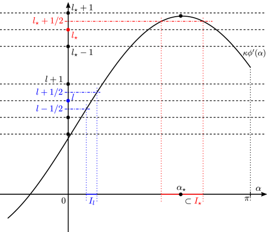
Given $r\in\mathbb{R}$, let $\lfloor r\rfloor$ denote the floor function, i.e. the integer $n\in\mathbb{Z}$ such that $n\leq r<n+1$. Denote (Figure 1)

$$l_{\star}(m):=\lfloor\kappa\phi^{\prime}(\alpha_{\star})\rfloor,\ m\not=0.$$ (4.13)

Note that $\kappa\phi^{\prime}(\alpha_{\star})$ is not an integer for any $m\in\mathbb{Z}$, because $|\kappa\phi^{\prime}(\alpha_{\star})|=|m\kappa x_{0}|$ is irrational (see Assumption 2.4(1)). Consider the set of integers

$$L(m):=\{l\in\mathbb{Z}:\,l=\kappa\phi^{\prime}(\alpha)\text{ for some }|\alpha|\leq\pi\},\ m\not=0.$$ (4.14)

Clearly, $l\in L(m)$ is equivalent to $|l|\leq l_{\star}(m)$. Define the set

$$\begin{split}&I_{\star}=\{|\alpha|\leq\pi:|\kappa\phi^{\prime}(\alpha)|\geq l_{\star}(m)+(1/2)\}.\end{split}$$ (4.15)

An illustration of one part of $I_{\star}$, namely the interval $\{|\alpha|\leq\pi:\kappa\phi^{\prime}(\alpha)\geq l_{\star}(m)+(1/2)\}$, is shown in red in Figure 1. The other interval $\{|\alpha|\leq\pi:\kappa\phi^{\prime}(\alpha)\leq-(l_{\star}(m)+(1/2))\}$ is not visible. It is possible that $I_{\star}$ is empty. Additionally, consider the sets:

$$\begin{split}&I_{l}:=\{\alpha\in[-\pi,\pi]:|\kappa\phi^{\prime}(\alpha)-l|\leq 1/2\},\ |l|\leq l_{\star}(m),\end{split}$$ (4.16)

see a blue interval in Figure 1. Again, the second part of $I_{l}$, which is a subset of $[-\pi,0]$, is not visible. For simplicity of notation, the dependence of the sets $I_{\star}$ and $I_{l}$ on $m$ is omitted. Each $I_{l}$ is the union of at most three intervals. As is easily seen, each subinterval that makes up $I_{l}$ satisfies the assumptions of Lemma 4.3. By construction,

$$\cup_{|l|\leq l_{\star}(m)}I_{l}\cup I_{\star}=[-\pi,\pi].$$ (4.17)

The intervals that make up $I_{l}$ are ‘regular’ in the sense that each of them satisfies the assumptions of Lemma 4.3, so the corresponding integrals can be estimated using (4.11). Each of the two intervals that make up $I_{\star}$ is ‘exceptional’: (4.11) does not apply to them, because there is no $l$ such that $\kappa\phi^{\prime}(\alpha_{0})=l$ for some $\alpha_{0}\in I_{\star}$. Thus, in addition to the regular sets $I_{l}$, we have to consider the exceptional set $I_{\star}$. Since Lemma 4.3 does not apply to $I_{\star}$, estimation of its contribution requires special handling. The following two lemmas are proven in Appendix C.

Lemma 4.4.

Under the assumptions of Theorem 2.5 one has

$$\begin{split}\epsilon\sum_{1\leq|m|\leq\epsilon^{-\gamma}}\biggl{|}\sum_{\alpha_{k}\in I_{\star}}\tilde{g}_{m}(\alpha_{k})e\biggl{(}\frac{\phi(\alpha_{k})}{\epsilon}\biggr{)}\biggr{|}&=O(\epsilon)\text{ if }M>\nu+1.\end{split}$$ (4.18)

Let the right side of (4.11), where $g$ is replaced by $\tilde{g}_{m}$, be denoted $W_{l,m}$. Then we have the following lemma.

Lemma 4.5.

Under the assumptions of Theorem 2.5 one has

$$\sum_{1\leq|m|\leq\epsilon^{-\gamma}}\sum_{|l|\in l_{\star}(m)}W_{l,m}=O(\epsilon^{1/2})\text{ if }M>\max((\nu+7)/4,5/2).$$ (4.19)

Combining (4.18) and (4.19) finishes the proof of (3.4).

5 Numerical experiments

In this section, we present numerical experiments to verify the main results in section 2. To do this, we apply (2.6) to simulated noise draws, $\eta_{k,j}$, under the assumption that the useful signal is zero (see section 2).

In the examples presented here, the entries $\eta_{k,j}:=\eta(\alpha_{k},p_{j})$ are drawn from a uniform distribution with mean zero and variance

$$\sigma^{2}(\alpha,p)=(1/3)u(\alpha,p),\ u(\alpha,p):=[1+(1/2)\sin(\alpha)][1+(1/2)\sin(\pi p)].$$ (5.1)

Specifically, we drew random numbers uniformly on $[-1,1]$ using the Matlab function “rand,” and scaled these by $\sqrt{u(\alpha,p)}$ to generate $\eta_{k,j}$ with sample variance $\sigma^{2}$ as in (5.1). Throughout the simulations presented, we set $\epsilon=1/j_{m}$, where $j_{m}\geq 1$ is the sampling rate, and $\kappa$ (as in (2.1)) is set to $\kappa=2\pi$. The reconstruction space is $[-1,1]^{2}$, $p_{j}=-1+(j-1)/j_{m}$, $1\leq j\leq 2j_{m}+1$, and $\alpha_{k}=2\pi\frac{k}{j_{m}}$, for $1\leq k\leq j_{m}$.

(a) reconstruction on $[-1,1]^{2}$

(b) reconstruction on $[-\epsilon,\epsilon]^{2}$

Figure 2: Example image reconstructions from uniform random noise with $j_{m}=10^{3}$ on the full scale (a), and within an $\epsilon$ neighborhood of zero (b).

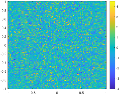
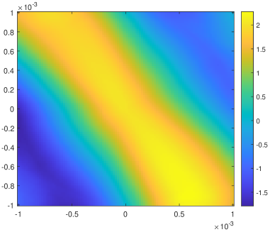
For reconstruction, we use (2.6), where $\varphi$ is the Keys kernel [21]. See figures 2(a) and 2(b), where we have shown example image reconstructions from a uniform noise draw (as detailed above) on the full image scale (i.e., $[-1,1]^{2}$), and within an $\epsilon$ neighborhood of zero, respectively. The image in figure 2(a) is noisy and the pixel values appear to vary independently. In contrast, in figure 2(b), the image appears smooth. This is in line with Theorem 2.9.

(a) observed pdf (histogram)

(b) predicted pdf

(c) covariance error with $\epsilon$

Figure 3: Observed (a) and predicted (b) pdf functions for $x_{0}=\frac{1}{4}(\sqrt{2},\sqrt{3})$ and $x_{1}=x_{0}+\frac{\epsilon}{2\sqrt{2}}(1,1)$, with $j_{m}=10^{3}$ and $n=10^{4}$ samples. (c) - covariance error as a function of $\epsilon$; $n=10^{4}$ samples were used to calculate the covariance error for all values of $\epsilon$ in the plot in (c).

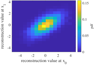
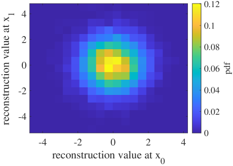
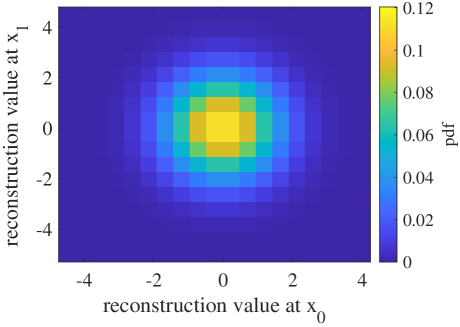
We now aim to evaluate the accuracy of the covariance predictions provided by (2.13), and show that the reconstructed values in any $O{(\epsilon)}$ size neighborhood follow a Gaussian distribution. To do this, we simulate $n=10^{4}$ image reconstructions as in figure 2(b) and calculate the covariance matrix and histogram between two fixed points, $x_{0}$ and $x_{1}$ within an $\epsilon$ neighborhood, and match this to the predictions given by $\text{Cov}(\check{x},\check{y})$ in (2.13). In figure 3(a), we show the observed pdf function (calculated using a histogram) which corresponds to $x_{0}=\frac{1}{4}(\sqrt{2},\sqrt{3})$ and $x_{1}=x_{0}+(\epsilon/2)\check{x}$, where $\check{x}=(1/\sqrt{2})(1,1)$ and $\epsilon=10^{-3}$. This matches well with the predicted Gaussian pdf in figure 3(b), and the least squares error is $\|P_{o}-P\|_{2}/\|P_{o}\|_{2}=0.07$, where $P_{o}$ and $P$ denote the vectorized images in figures 3(a) and 3(b), respectively. The observed covariance matrix, $C_{o}$, and the predicted covariance matrix, $C$, are computed to be

$$C_{o}=\begin{pmatrix}1.34&0.86\\ 0.86&1.36\end{pmatrix},\quad C=\begin{pmatrix}\text{Cov}(0,0)&\text{Cov}(0,\check{x}/2)\\ \text{Cov}(\check{x}/2,0)&\text{Cov}(0,0)\end{pmatrix}=\begin{pmatrix}1.36&0.86\\ 0.86&1.36\end{pmatrix},$$ (5.2)

where Cov and $C$ are calculated using (2.13). We see that $C_{o}$ and $C$ are very close, and the error is $\|C-C_{o}\|_{F}/\|C_{o}\|_{F}=0.01$. The observed mean is $(-0.0148,0.0003)$, which is close to zero as expected since the $\eta_{k,j}$ were drawn from a uniform distribution with mean zero. In this example, $x_{1}$ is fairly close to $x_{0}$ (i.e., within distance $\epsilon/2$), as in figure 2(b), and they have highly correlated reconstructed values.

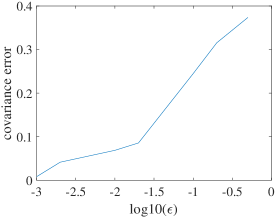
We note that these results are only valid as $\epsilon\to 0$. To illustrate this, see figure 3(c), where we have plotted the covariance error (computed using Frobenius norm and the same $x_{0}$ and $x_{1}$ points as before) against $\epsilon$. The error is increasing with $\epsilon$, and becomes $>20\%$ when $\epsilon>0.1$ is of a significant size relative to the size of the scanning region (i.e., $[-1,1]^{2}$). In this case, $\epsilon=0.1$ is $5\%$ of the scanning region width.

(a) observed pdf (histogram)

(b) predicted pdf

Figure 4: Observed (a) and predicted (b) pdf functions for $x_{0}=\frac{1}{4}(\sqrt{2},\sqrt{3})$ and $x_{1}=x_{0}+\frac{5\epsilon}{\sqrt{2}}(1,1)$, with $j_{m}=10^{3}$ and $n=10^{4}$ samples.

In the results thus far, the chosen $x_{0}$ and $x_{1}$ were within the same $\epsilon$ neighborhood. For $\epsilon$ small enough, (by Theorem 2.9), (2.13) holds for pairs of points in larger regions relative to the size of $\epsilon$. To validate this, we keep $x_{0}$ and $\check{x}$ the same as before, set $x_{1}=x_{0}+5\epsilon\check{x}$ with $\epsilon=10^{-3}$, and calculate the observed and predicted pdf functions as in figure 3. We use a sample size of $n=10^{4}$, as in the previous example. See figure 4 for our results. The pdf functions presented in figures 4(a) and 4(b) match up well, and the least squares error is $\|P_{o}-P\|_{2}/\|P_{o}\|_{2}=0.07$, where $P_{o}$ and $P$ denote the vectorized images in figures 4(a) and 4(b), respectively, as before. The observed covariance matrix, $C_{o}$, which corresponds to figure 4(a), and predicted covariance matrix, $C$, which corresponds to figure 4(b), are as follows.

$$C_{o}=\begin{pmatrix}1.31&-0.003\\ -0.003&1.32\end{pmatrix},\quad C=\begin{pmatrix}\text{Cov}(0,0)&\text{Cov}(0,5\check{x})\\ \text{Cov}(5\check{x},0)&\text{Cov}(0,0)\end{pmatrix}=\begin{pmatrix}1.36&-0.002\\ -0.002&1.36\end{pmatrix}.$$ (5.3)

The error again is quite small: $\|C-C_{o}\|_{F}/\|C_{o}\|_{F}=0.04$. The observed mean is $(-0.01,-0.01)$, which is near zero as predicted. In this case, $x_{0}$ and $x_{1}$ are distance $5\epsilon$ apart and have relatively uncorrelated reconstructed values when compared to the previous example where $|x_{0}-x_{1}|=\epsilon/2$.

The above examples validate our theory and provide accurate predictions for the noise distribution in 2D CT reconstruction in small neighborhoods, e.g., in this case up to size $5\epsilon$.

Appendix A Proof of approximation in equations (3.3) and (3.10).

Note that (3.3) is a particular case of (3.10) with $\check{x}=\check{x}_{i_{1}}=\check{x}_{i_{2}}$, $i_{1},i_{2}\in 1,\dots,K$, and $\vec{\theta}=(1,0,\dots,0)$, so we prove only (3.10). Clearly,

$$\Delta\alpha\sum_{j,k}\mathcal{H}\varphi^{\prime}(a_{k}-j+\vec{\alpha}_{k}\cdot\check{x}_{i_{1}})\mathcal{H}\varphi^{\prime}(a_{k}-j+\vec{\alpha}_{k}\cdot\check{x}_{i_{2}})\sigma^{2}(\alpha_{k},p_{j})={S}_{1}+{S}_{2},$$ (A.1)

where $a_{k}$ are given in (3.11) and

$${S}_{1} =\Delta\alpha\sum_{j,k}\mathcal{H}\varphi^{\prime}(a_{k}-j+\vec{\alpha}_{k}\cdot\check{x}_{i_{1}})\mathcal{H}\varphi^{\prime}(a_{k}-j+\vec{\alpha}_{k}\cdot\check{x}_{i_{2}})\big{(}\sigma^{2}(\alpha_{k},p_{j})-\sigma^{2}(\alpha_{k},\vec{\alpha}_{k}\cdot x_{0})\big{)},$$

$${S}_{2} =\Delta\alpha\sum_{j,k}\mathcal{H}\varphi^{\prime}(a_{k}-j+\vec{\alpha}_{k}\cdot\check{x}_{i_{1}})\mathcal{H}\varphi^{\prime}(a_{k}-j+\vec{\alpha}_{k}\cdot\check{x}_{i_{2}})\sigma^{2}(\alpha_{k},\vec{\alpha}_{k}\cdot x_{0}).$$

Let us define:

$${\Phi}(a,t_{1},t_{2})=\sum_{j}\lvert\mathcal{H}\varphi^{\prime}(a-j+t_{1})\mathcal{H}\varphi^{\prime}(a-j+t_{2})(a-j)\rvert.$$

Using that $\sigma\in C^{1}([-\pi,\pi]\times[-P,P])$ (Assumption 2.1(2)) and the property $\mathcal{H}\varphi^{\prime}(t)=O(t^{-2})$, $t\to\infty$, we bound $S_{1}$ by:

$$\lvert{S}_{1}\rvert\leq c\epsilon\Delta\alpha\sum_{\lvert\alpha_{k}\rvert\leq\pi}{\Phi}(a_{k},\vec{\alpha}_{k}\cdot\check{x}_{i_{1}},\vec{\alpha}_{k}\cdot\check{x}_{i_{2}})=O(\epsilon).$$ (A.2)

Using (A.1) and (A.2) in the expression for $\mathbb{E}\xi^{2}_{\epsilon}$, we get (3.10).

Appendix B Proof of Lemma 4.3 and auxiliary results

B.1 Proof of Lemma 4.3

We may assume without loss of generality that $\phi_{l}(\alpha_{0})=0$ in (4.11). Otherwise, this can be achieved by subtracting $\phi_{l}(\alpha_{0})$ from $\phi_{l}(\alpha)$ in the exponent and not changing the value on the left. Then $\phi_{l}(\alpha)$ does not change sign on $I$. We may assume without loss of generality that $\phi_{l}(\alpha)\geq 0$ on $I$. Define the function $E(\alpha):=\int_{0}^{\alpha}e(t^{2})\text{d}t$. Using the definition of $h_{l}$ (see (4.9)):

$$\begin{split}&J:=\int_{I}g(\alpha)h_{l}(\alpha)e\biggl{(}\frac{\phi_{l}(\alpha)}{\epsilon}\biggr{)}\text{d}\alpha=2\pi\kappa\epsilon^{1/2}\int_{I}\frac{g(\alpha)\phi_{l}^{1/2}(\alpha)}{\sin(\pi\kappa\phi^{\prime}(\alpha))}\text{d}E((\phi_{l}(\alpha)/\epsilon)^{1/2}).\end{split}$$ (B.1)

Since $|E(t)|$ is bounded on $\mathbb{R}$, integrating by parts gives

$$\begin{split}&|J|\leq c\epsilon^{1/2}\biggl{[}\max_{\alpha\in I}\bigg{|}\frac{g(\alpha)\phi_{l}^{1/2}(\alpha)}{\sin(\pi\kappa\phi^{\prime}(\alpha))}\bigg{|}+\int_{I}\bigg{|}\bigg{[}\frac{g(\alpha)\phi_{l}^{1/2}(\alpha)}{\sin(\pi\kappa\phi^{\prime}(\alpha))}\bigg{]}^{\prime}\bigg{|}\text{d}\alpha.\end{split}$$ (B.2)

The following lemma is proven in appendix B.2.

Lemma B.1.

The function $f(\alpha):=[\phi_{l}^{1/2}(\alpha)/\sin(\pi\kappa\phi^{\prime}(\alpha))]^{\prime}$ may change sign at most finitely many times on $I$ uniformly in $m\not=0$.

Using the last lemma in (B.2) gives

$$\begin{split}&|J|\leq c\epsilon^{1/2}\biggl{[}g_{\text{mx}}(I)+\int_{I}|g^{\prime}(\alpha)|\text{d}\alpha\biggr{]}\max_{\alpha\in I}\bigg{|}\frac{\phi_{l}^{1/2}(\alpha)}{\sin(\pi\kappa\phi^{\prime}(\alpha))}\bigg{|}.\end{split}$$ (B.3)

Since $|\kappa\phi^{\prime}(\alpha)|\leq 1/2$, $\alpha\in I$,

$$\begin{split}\max_{\alpha\in I}\bigg{|}\frac{\phi_{l}^{1/2}(\alpha)}{\sin(\pi\kappa\phi^{\prime}(\alpha))}\bigg{|}\leq c\max_{\alpha\in I}\bigg{|}\frac{\phi_{l}^{1/2}(\alpha)}{\phi^{\prime}(\alpha)}\bigg{|}\leq c\big{(}\phi^{\prime\prime}(\alpha_{l}^{*})\big{)}^{-1/2}.\end{split}$$ (B.4)

Here we used the following lemma with $f(\alpha)=\phi_{l}(\alpha)$.

Lemma B.2.

If $I$ be an interval such that $\sin\alpha\not=0$ for any $\alpha$ in its interior. Define

$$f(\alpha):=\sin\alpha-\sin\alpha_{0}-\cos\alpha_{0}(\alpha-\alpha_{0})$$ (B.5)

for some $\alpha_{0}\in I$ such that $\sin\alpha_{0}\not=0$. One has

$$\max_{\alpha\in I}[|f(\alpha)|/(f^{\prime}(\alpha))^{2}]\leq c|f^{\prime\prime}(\alpha_{0})|^{-1}.$$ (B.6)

Lemma B.2 is proven in appendix B.3. Note that (B.6) applies to $\phi_{l}$ because the inequality in (B.6) does not change if $f$ is replaced by $cf$ and we can shift the argument $\alpha-\alpha_{\star}\to\alpha$. See also the first two sentences in this subsection.

Combining (B.1)–(B.4) finishes the proof of lemma 4.3.

B.2 Proof of Lemma B.1

To prove the lemma we show that there are finitely many solutions to the equation $f(\alpha)=0$, $\alpha\in I$, uniformly in $m\not=0$. By simple calculations, we get that these solutions are obtained by solving

$$\frac{\tan(\pi\kappa\phi^{\prime}_{l}(\alpha))}{\pi\kappa\phi^{\prime}_{l}(\alpha)}=2\frac{\phi_{l}(\alpha)\phi_{l}^{\prime\prime}(\alpha)}{(\phi^{\prime}_{l}(\alpha))^{2}},\ \alpha\in I.$$ (B.7)

Set

$$v(\alpha):=(\vec{\alpha}-\vec{\alpha}_{0})\cdot x_{0}-(\vec{\alpha}_{0}^{\perp}\cdot x_{0})(\alpha-\alpha_{0}).$$ (B.8)

Recall that by our convention, $\partial_{\alpha}\vec{\alpha}=\vec{\alpha}^{\perp}$. Clearly, $v(\alpha)$ is an entire function of $\alpha\in\mathbb{C}$. By (4.9), $\phi_{l}(\alpha)-\phi_{l}(\alpha_{0})\equiv-mv(\alpha)$, $\alpha\in I$. Then (B.7) becomes

$$\frac{\tan(m\pi v^{\prime}(\alpha))}{m\pi v^{\prime}(\alpha)}=2\frac{v(\alpha)v^{\prime\prime}(\alpha)}{(v^{\prime}(\alpha))^{2}},\ \alpha\in I.$$ (B.9)

By assumption, $v^{\prime\prime}(\alpha)\not=0$ in the interior of $I$. Hence we can express both sides of (B.9) as functions of $s=mv^{\prime}(\alpha)$ to obtain

$$\frac{\tan(\pi s)}{\pi s}-1=v_{1}(s/m)-1,\ |s|\leq 1/2.$$ (B.10)

The inequality $|s|\leq 1/2$ follows from assumption 3 of Lemma 4.3. Both sides of (B.10) are analytic near $s=0$ and equal zero at $s=0$ (i.e., $\alpha=\alpha_{0}$). As $m\to\infty$, the right-hand side converges uniformly to zero. The left-hand side equals zero only near $s=0$. Hence, for large $|m|$, all solutions to (B.10) are located near $s=0$. Expanding both sides near $s=0$ gives

$$c_{1}s^{2}(1+O(s^{2}))=c_{2}(s/m)^{k}(1+O(|s/m|)),\ s\to 0.$$ (B.11)

Here $c_{1},c_{2}\not=0$, and $k\geq 1$ is the index of the first non-zero term in the expansion of $h_{1}-1$. If $k\geq 2$, the equation has no solutions if $|m|\gg 1$. In the remaining case we get the equation

$$s=c/m+O(|s/m|+|s|^{3})\text{ if }k=1,$$ (B.12)

for some $c\not=0$. Therefore, if $|m|$ is sufficiently large, there is one solutions if $k=1$ and no solutions - if $k\geq 2$. If $|m|$ is bounded, the number of solutions is bounded as well since (B.7) is an equality of two analytic functions.

B.3 Proof of Lemma B.2

Without loss of generality we can assume that $I\subset[0,\pi]$, $f^{\prime\prime}(\alpha)<0$ and, therefore, $f(\alpha)\leq 0$ on $I$. Then (B.6) becomes

$$\frac{\sin\alpha_{0}+\cos\alpha_{0}(\alpha-\alpha_{0})-\sin\alpha}{(\cos\alpha_{0}-\cos\alpha)^{2}}\leq c\frac{1}{\sin\alpha_{0}},\quad 0<\alpha,\alpha_{0}<\pi.$$ (B.13)

The denominator on the left can be zero only when $\alpha=\alpha_{0}$. Hence we consider the case $|h|\ll 1$, where $h=\alpha-\alpha_{0}$. Writing $\alpha=\alpha_{0}+h$ and ignoring irrelevant constants gives

$$\frac{\sin\alpha_{0}(1-\cos h)+\cos\alpha_{0}(h-\sin h)}{h^{2}\sin^{2}((\alpha+\alpha_{0})/2)}\leq c\frac{1}{\sin\alpha_{0}},\quad 0<\alpha,\alpha_{0}<\pi,\ |\alpha-\alpha_{0}|\ll 1.$$ (B.14)

Thus, suffices it to prove the following two inequalities

$$\frac{\sin^{2}\alpha_{0}}{\sin^{2}((\alpha+\alpha_{0})/2)}\leq c,\ \frac{|\alpha-\alpha_{0}|\sin\alpha_{0}}{\sin^{2}((\alpha+\alpha_{0})/2)}\leq c,\quad 0<\alpha,\alpha_{0}<\pi,\ |\alpha-\alpha_{0}|\ll 1.$$ (B.15)

The denominator may approach zero only if $\alpha,\alpha_{0}\to 0$ or $\alpha,\alpha_{0}\to\pi$. The two cases are analogous, so we only consider the former. The two inequalities now easily follow from the following inequalities:

$$\frac{\alpha_{0}^{2}}{(\alpha+\alpha_{0})^{2}}\leq 1,\ \frac{|\alpha-\alpha_{0}|\alpha_{0}}{(\alpha+\alpha_{0})^{2}}\leq 1,\quad\alpha,\alpha_{0}>0.$$ (B.16)

Appendix C Proofs of Lemma 4.4 and 4.5

C.1 Proof of Lemma 4.4

Suppose that $\alpha_{\star}$ satisfies $\phi^{\prime\prime}(\alpha_{\star})=0$, $\alpha_{\star}$ is a local maximum of $\phi^{\prime}(\alpha)$ and $l_{\star}=\lfloor\kappa\phi^{\prime}(\alpha_{\star})\rfloor$. The dependence of $l_{\star}$ on $m$ is omitted for simplicity. The sets $\{|\alpha|\leq\pi:\kappa\phi^{\prime}(\alpha)\geq l_{\star}+(1/2)\}$ and $\{|\alpha|\leq\pi:\kappa\phi^{\prime}(\alpha)\leq-(l_{\star}+(1/2))\}$ are completely analogous. Therefore, in this section we consider only the former and denote it $I_{\star}$.

Even though $\kappa\phi^{\prime}(\alpha)$ may take the value $l_{\star}$ at two points (on either side of $\alpha_{\star}$), in this section we assume that $\alpha_{l_{\star}}^{*}$ is the smaller of the two (i.e., $\alpha_{l_{\star}}^{*}<\alpha_{\star}$). If $I_{\star}\not=\varnothing$, there exists $\alpha_{h}<\alpha_{\star}$ such that $\kappa\phi^{\prime}(\alpha_{h})=l_{\star}+(1/2)$. Split $I_{\star}$ into two intervals $[\alpha_{h},\alpha_{\star}]$ and $[\alpha_{\star},2\alpha_{\star}-\alpha_{h}]$. The two intervals are completely analogous, so we prove (4.18) by restricting the interior sum to $\alpha_{k}\in[\alpha_{h},\alpha_{\star}]$.

The sum with respect to $\alpha_{k}\in[\alpha_{h},\alpha_{\star}]$ reduces to an integral over $[\alpha_{h},\alpha_{\star}]$ by using $l=l_{\star}+1$ in (4.10). Note that Lemma 4.2 applies regardless of whether there exists an $\alpha\in I$ such that $\kappa\phi^{\prime}(\alpha)=l$. The following lemma proves Lemma 4.4.

Lemma C.1.

Under the assumptions of Theorem 2.5, one has

$$\begin{split}\sum_{1\leq|m|\leq\epsilon^{-\gamma}}&\biggl{|}\int_{\alpha_{h}}^{\alpha_{\star}}(\tilde{g}_{m}h_{l_{\star}+1})(\alpha)e\biggl{(}\frac{\phi_{l_{\star}+1}(\alpha)}{\epsilon}\biggr{)}\text{d}\alpha\biggr{|}=O(\epsilon)\text{ if }M>\nu+1.\end{split}$$ (C.1)

Proof.

Let $J$ be the integral in (C.1). Integration by parts in (C.1) gives:

$$\begin{split}|J|&\leq c\epsilon(J_{1}+J_{2}),\\ J_{1}&:=\frac{|\tilde{g}_{m}(\alpha_{\star})|}{|\sin(\pi\kappa\phi_{l_{\star}+1}^{\prime}(\alpha_{\star}))|}+\frac{|\tilde{g}_{m}(\alpha_{h})|}{|\sin(\pi\kappa\phi_{l_{\star}+1}^{\prime}(\alpha_{h}))|},\ J_{2}:=\int_{\alpha_{h}}^{\alpha_{\star}}\biggl{|}\partial_{\alpha}\frac{\tilde{g}_{m}(\alpha)}{\sin(\pi\kappa\phi_{l_{\star}+1}^{\prime}(\alpha))}\biggr{|}\text{d}\alpha.\end{split}$$ (C.2)

By (4.12),

$$\begin{split}-\kappa\phi_{l_{\star}+1}^{\prime}(\alpha)=&-Qm\cos(\alpha-\alpha_{\star})+(l_{\star}+1)=Qm(1-\cos(\alpha-\alpha_{\star}))-Qm+(l_{\star}+1)\\ =&\Delta+Qm(1-\cos(\alpha-\alpha_{\star})),\ \Delta:=\lceil Qm\rceil-Qm,\ l_{\star}=\lfloor Qm\rfloor,\ \alpha\in I_{\star},\end{split}$$ (C.3)

where $\lceil r\rceil:=1-\lfloor r\rfloor$ is the ceiling function. Since $\kappa|\phi_{l_{\star}}^{\prime}(\alpha_{h})|=\kappa|\phi_{l_{\star}+1}^{\prime}(\alpha_{h})|=1/2$, (4.3) implies

$$\begin{split}J_{1}\leq c\rho(m)\langle m\kappa\vec{\alpha}_{\star}^{\perp}\cdot x_{0}\rangle^{-1}.\end{split}$$ (C.4)

Also, by (4.3) and (C.3),

$$\begin{split}J_{2}&\leq c\rho(m)\bigg{(}\int_{\alpha_{h}}^{\alpha_{\star}}\frac{|m|}{|\sin(\pi\kappa\phi_{l_{\star}+1}^{\prime}(\alpha))|}\text{d}\alpha+\biggl{|}\int_{\alpha_{h}}^{\alpha_{\star}}\partial_{\alpha}\frac{1}{\sin(\pi\kappa\phi_{l_{\star}+1}^{\prime}(\alpha))}\text{d}\alpha\biggr{|}\bigg{)}\\ &\leq c\rho(m)\bigg{(}\int_{\alpha_{h}}^{\alpha_{\star}}\frac{|m|\text{d}\alpha}{\Delta+Qm(1-\cos(\alpha-\alpha_{\star}))}+\frac{1}{|\phi_{l_{\star}}^{\prime}(\alpha_{\star})|}\bigg{)}\\ &\leq c\rho(m)\big{[}(|m|/\langle m\kappa\vec{\alpha}_{\star}^{\perp}\cdot x_{0}\rangle)^{1/2}+\langle m\kappa\vec{\alpha}_{\star}^{\perp}\cdot x_{0}\rangle^{-1}\big{]}\leq c\frac{\rho(m)}{\langle m\kappa\vec{\alpha}_{\star}^{\perp}\cdot x_{0}\rangle}.\end{split}$$ (C.5)

In the first line we used that $|\kappa\phi_{l_{\star}+1}^{\prime}(\alpha)|\leq 1/2$, $\alpha\in[\alpha_{h},\alpha_{\star}]$, and the functions $\cos(\pi\kappa\phi_{l_{\star}+1}^{\prime}(\alpha))$ and $\phi^{\prime\prime}(\alpha)\equiv\phi_{l_{\star}+1}^{\prime\prime}(\alpha)$ do not change sign on that interval. Thus, the bounds for $J_{1}$ and $J_{2}$ are the same. Adding these bounds over $1\leq|m|\leq e^{-\gamma}$ we see that the sum is finite if $M>\nu+1$. ∎

C.2 Proof of Lemma 4.5

Throughout this subsection, $\alpha_{r}^{*}$ denote locally unique solutions of $\kappa\phi^{\prime}(\alpha)=r$, $|r|\leq|m\kappa x_{0}|$.

From (4.3) and (4.11),

$$\biggl{|}\int_{I}g(\alpha)h_{l}(\alpha)e\biggl{(}\frac{\phi_{l}(\alpha)}{\epsilon}\biggr{)}\text{d}\alpha\biggr{|}\leq W_{l,m}\leq c\frac{\rho(m)|m|\epsilon^{1/2}}{(\phi^{\prime\prime}(\alpha_{l}^{*}))^{1/2}},\ m\not=0.$$ (C.6)

We sum the right-hand side of (C.6) over $|l|\leq l_{\star}(m)$ and then over $1\leq|m|\leq\epsilon^{-\gamma}$. Begin by looking at the sums $\sum_{|l|\leq l_{\star}(m)}(\phi^{\prime\prime}(\alpha_{l}^{*}))^{-1/2}$. Recall that (see Figure 1),

$$I_{l}=[\alpha_{l-(1/2)}^{*},\alpha_{l+(1/2)}^{*}],\ |l|<l_{\star};\ I_{l}=\begin{cases}[\alpha_{l-(1/2)}^{*},\alpha_{l+(1/2)}^{*}],&|l|=l_{\star},I_{\star}\not=\varnothing,\\ [\alpha_{l_{\star}-(1/2)}^{*},\alpha_{\star}],&l=l_{\star},I_{\star}=\varnothing,\\ [\alpha_{\star},\alpha_{l_{\star}+(1/2)}^{*}],&l=-l_{\star},I_{\star}=\varnothing.\end{cases}$$ (C.7)

Even if $I_{\star}=\varnothing$ and $\alpha_{\star}\in I_{l_{\star}}$, Lemma 4.3 still applies (e.g., condition 1 of the lemma is not violated even though $\phi^{\prime\prime}(\alpha_{\star})=0$) because $\alpha_{\star}$ is an endpoint of $I_{l_{\star}}$, it is not in the interior of $I_{l_{\star}}$. The same applies to $I_{-l_{\star}}$.

By (4.12),

$$\begin{split}|\phi^{\prime\prime}(\alpha_{l}^{*})|&=\big{[}(Qm)^{2}-l^{2}\big{]}^{1/2}\geq c|m|^{1/2}\begin{cases}\langle m\kappa\vec{\alpha}_{\star}^{\perp}\cdot x_{0}\rangle^{1/2},&|l|=l_{\star},\\ (l_{\star}-|l|)^{1/2},&|l|<l_{\star}.\end{cases}\end{split}$$ (C.8)

Then,

$$\begin{split}\sum_{|l|\leq l_{\star}(m)}\frac{1}{(\phi^{\prime\prime}(\alpha_{l}^{*}))^{1/2}}&\leq\frac{c}{|m|^{1/4}}\biggl{[}\langle m\kappa\vec{\alpha}_{\star}^{\perp}\cdot x_{0}\rangle^{-1/4}+\sum_{l=0}^{l_{\star}-1}(l_{\star}-l)^{-1/4}\biggr{]}\\ &\leq c|m|^{-1/4}\bigl{[}\langle m\kappa\vec{\alpha}_{\star}^{\perp}\cdot x_{0}\rangle^{-1/4}+|m|^{3/4}\bigr{]},\end{split}$$ (C.9)

and

$$\begin{split}\sum_{1\leq|m|\leq\epsilon^{-\gamma}}&\frac{\rho(m)|m|}{|m|^{1/4}}\bigl{[}\langle m\kappa\vec{\alpha}_{\star}^{\perp}\cdot x_{0}\rangle^{-1/4}+|m|^{3/4}\bigr{]}\leq c,\quad M>\max((\nu+7)/4,5/2).\end{split}$$ (C.10)

Consequently, (cf. (C.6))

$$\sum_{1\leq|m|\leq\epsilon^{-\gamma}}\sum_{|l|\leq l_{\star}(m)}W_{l,m}=O(\epsilon^{1/2}),\ M>\max((\nu+7)/4,5/2),$$ (C.11)

and Lemma 4.5 is proven.

References Cited

- [1] Robert J. Adler. The Geometry of Random Fields. Society for Industrial and Applied Mathematics, Philadelphia, PA, 2010.
- [2] Krishna B. Athreya and Soumendra N. Lahiri. Measure theory and probability theory. Springer, New York, NY, springer m edition, 2006.
- [3] Nicolai Bissantz, Hajo Holzmann, and Katharina Proksch. Confidence regions for images observed under the Radon transform. Journal of Multivariate Analysis, 128:86–107, 2014.
- [4] L. Cavalier. Asymptotically efficient estimation in a problem related to tomography. Math. Methods Statist., 7(4):445–456 (1999), 1998.
- [5] Laurent Cavalier. Efficient estimation of a density in a problem of tomography. Ann. Statist., 28(2):630–647, 2000.
- [6] Ashis Kumar Dhara, Sudipta Mukhopadhyay, Anirvan Dutta, Mandeep Garg, and Niranjan Khandelwal. A combination of shape and texture features for classification of pulmonary nodules in lung CT images. Journal of digital imaging, 29:466–475, 2016.
- [7] Ashis Kumar Dhara, Sudipta Mukhopadhyay, Pramit Saha, Mandeep Garg, and Niranjan Khandelwal. Differential geometry-based techniques for characterization of boundary roughness of pulmonary nodules in CT images. International journal of computer assisted radiology and surgery, 11:337–349, 2016.
- [8] Sarah E. Divel and Norbert J. Pelc. Accurate Image Domain Noise Insertion in CT Images. IEEE Transactions on Medical Imaging, 39(6):1906–1916, 2020.
- [9] A. Faridani. Sampling theory and parallel-beam tomography. In Sampling, wavelets, and tomography, volume 63 of Applied and Numerical Harmonic Analysis, pages 225–254. Birkhauser Boston, Boston, MA, 2004.
- [10] F D Gakhov. Boundary Value Problems. Pergamon Press, Oxford, 1966.
- [11] David Gilbarg and Neil S. Trudinger. Elliptic Partial Differential Equations of Second Order. Springer, Berlin, Heidelberg, 2001.
- [12] Alexander Katsevich. A local approach to resolution analysis of image reconstruction in tomography. SIAM Journal on Applied Mathematics, 77(5):1706–1732, 2017.
- [13] Alexander Katsevich. Analysis of reconstruction from discrete Radon transform data in when the function has jump discontinuities. SIAM Journal on Applied Mathematics, 79:1607–1626, 2019.
- [14] Alexander Katsevich. Analysis of resolution of tomographic-type reconstruction from discrete data for a class of distributions. Inverse Problems, 36(12), 2020.
- [15] Alexander Katsevich. Resolution analysis of inverting the generalized Radon transform from discrete data in . SIAM Journal of Mathematical Analysis, 52(4):3990–4021, 2020.
- [16] Alexander Katsevich. Analysis of tomographic reconstruction of objects in with rough edges. arXiv, (2312.08259 [math.NA]), 2023.
- [17] Alexander Katsevich. Analysis of view aliasing for the generalized Radon transform in . SIAM Journal on Imaging Sciences, to appear, 2023.
- [18] Alexander Katsevich. Novel resolution analysis for the Radon transform in for functions with rough edges. SIAM Journal of Mathematical Analysis, 55:4255–4296, 2023.
- [19] Alexander Katsevich. Resolution analysis of inverting the generalized -dimensional Radon transform in from discrete data. Journal of Fourier Analysis and Applications, 29, art. 6, 2023.
- [20] Alexander Katsevich. Resolution of 2D reconstruction of functions with nonsmooth edges from discrete Radon transform data. SIAM Journal on Applied Mathematics, 83(2):695–724, 2023.
- [21] R. G. Keys. Cubic Convolution Interpolation for Digital Image Processing. IEEE Transactions on Acoustics, Speech, and Signal Processing, ASSP-29(6):1153–1160, 1981.
- [22] Davar Khoshnevisan. Multiparameter Processes. An Introduction to Random Fields. Springer-Verlag, New York, 2002.
- [23] A. P. Korostelëv and A. B. Tsybakov. Optimal rates of convergence of estimators in a probabilistic setup of tomography problem. Problems of information transmission, 27:73–81, 1991.
- [24] A. P. Korostelëv and A. B. Tsybakov. Asymptotically minimax image reconstruction problems. In Topics in nonparametric estimation, volume 12 of Adv. Soviet Math., pages 45–86. Amer. Math. Soc., Providence, RI, 1992.
- [25] L Kuipers and H Niederreiter. Uniform Distribution of Sequences. Dover Publications, Inc., Mineola, NY, 2006.
- [26] François Monard, Richard Nickl, and Gabriel P. Paternain. Efficient nonparametric Bayesian inference for X-ray transforms. Ann. Statist., 47(2):1113–1147, 2019.
- [27] Francois Monard and Plamen Stefanov. Sampling the X-ray transform on simple surfaces. SIAM Journal on Mathematical Analysis, 53(3):1707–1736, 2023.
- [28] K. Naito. Classifications of irrational numbers and recurrent dimensions of quasi-periodic orbits. Journal of Nonlinear and Convex Analysis, 5(2):169–185, 2004.
- [29] F. Natterer. Sampling in Fan Beam Tomography. SIAM Journal on Applied Mathematics, 53:358–380, 1993.
- [30] V. P. Palamodov. Localization of harmonic decomposition of the Radon transform. Inverse Problems, 11:1025–1030, 1995.
- [31] S Siltanen, V Kolehmainen, S J Rvenp, J P Kaipio, P Koistinen, M Lassas, J Pirttil, and E Somersalo. Statistical inversion for medical X-ray tomography with few radiographs: I. general theory. Physics in Medicine and Biology, 48(10):1437–1463, may 2003.
- [32] P. Stefanov. Semiclassical sampling and discretization of certain linear inverse problems. SIAM Journal of Mathematical Analysis, 52:5554–5597, 2020.
- [33] Plamen Stefanov and Samy Tindel. Sampling linear inverse problems with noise. Asymptot. Anal., 132(3-4):331–382, 2023.
- [34] Simopekka Vänskä, Matti Lassas, and Samuli Siltanen. Statistical X-ray tomography using empirical Besov priors. Int. J. Tomogr. Stat., 11(S09):3–32, 2009.
- [35] Adam Wunderlich and Frédéric Noo. Image covariance and lesion detectability in direct fan-beam X-ray computed tomography. Physics in Medicine and Biology, 53(10):2471–2493, 2008.