Boundary layers in thermal convection are fluctuation-dominated
Abstract
We study the dynamics of thermal and momentum boundary layers in three-dimensional direct numerical simulations of Rayleigh-Bénard convection for the Rayleigh number range and . Using a Cartesian slab with horizontal periodic boundary conditions and an aspect ratio of 4, we obtain statistical homogeneity in the horizontal - and -directions, thus approximating an infinitely extended system. We observe that upon canonical use of long-time and area averages, a coherent mean flow is practically absent. Instead, the velocity field close to the wall is a collection of differently oriented local shear patches interspersed by shear-free, incoherent flow regions. These shear patches occupy an area fraction of approximately 40% for all . Rather than resulting in a pronounced mean with small fluctuations about it, the velocity field is dominated by strong fluctuations of all three components around a non-existent or weak mean. This feature is particularly pronounced for . We discuss the consequences of these observations for convection layers with larger aspect ratios, including boundary layer instabilities and the resulting turbulent heat transport.
I Introduction
Rayleigh-Bénard convection (RBC) is one of the fundamental flow configurations in fluid turbulence research. The fluid in this configuration is nominally confined to an infinitely extended layer enclosed between two parallel, horizontal and impermeable plates separated by a vertical distance (Rayleigh, 1916). When the fluid layer is heated sufficiently strongly from below (and cooled from above), buoyancy forces initiate a turbulent fluid motion that has a statistically preferred state with respect to the direction of gravity, . A central question concerns the amount of heat and momentum carried through the layer, and their dependencies on the imposed temperature difference between the top and bottom plates, . The temperature difference is expressed by the dimensionless Rayleigh number , where is the isobaric expansion coefficient, the kinematic viscosity, and the temperature diffusivity (Ahlers et al., 2009a; Chillà and Schumacher, 2012; Verma, 2018).
Since the RBC system is enclosed by walls at the top and bottom, the viscous and thermal boundary layers formed on these walls pose a bottleneck for the global transport of both heat and momentum. Their composition and dynamics at very high Rayleigh numbers still need to be better understood as emphasized recently (Iyer et al., 2020; Lindborg, 2023; Shishkina and Lohse, 2023; Creyssels and Martinard, 2024). For Rayleigh numbers , no laboratory experiment to-date has resolved the dynamic interplay of the boundary layers and their fluctuations with the basic structural elements, namely thermal plumes and shear layers. Direct numerical simulations (DNS) are thus the only way to compare their structure and statistical properties with predictions from theories for canonical laminar and turbulent boundary layers (Schlichting and Gersten, 2016). Furthermore, the closed-cell geometry of high-Rayleigh-number studies (Castaing et al., 1989; Chavanne et al., 1997; Niemela et al., 2000; Ahlers et al., 2009b; Urban et al., 2012) breaks the horizontal translation symmetry of the statistics, except possibly when the aspect ratio is very large (Pandey et al., 2018). Small aspect ratio enforces a dominant large-scale circulation (LSC) in the cell (Kadanoff, 2001), manifesting as a relatively coherent shear flow connecting the top and bottom plates, fluctuating only moderately in its mean orientation (Sreenivasan et al., 2002; Stevens et al., 2011; Shi et al., 2012; Scheel and Schumacher, 2017). Both aspects take us away from the original question on the heat and momentum transfer in an infinitely extended plane layer.
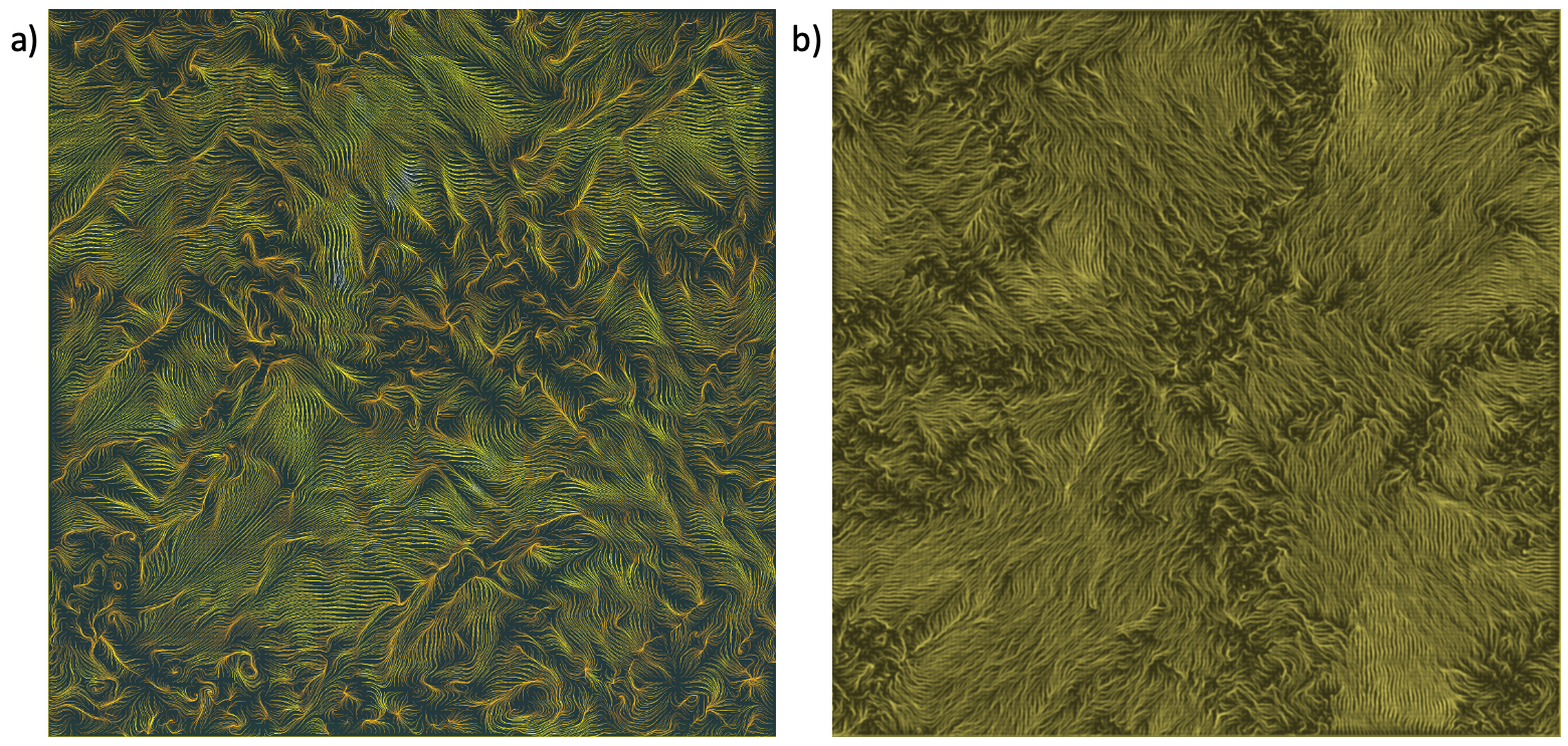
In this work, we focus on a configuration that is closer to the original RBC model of convection between a pair of infinitely extended planes, by using periodic boundaries in horizontal directions. Simulations with similar boundary conditions and Prandtl numbers have been done by Kerr (1996) for and , by Hartlep et al. (2003) for and , by van Reeuwijk et al. (2008) and van Reeuwijk and Jonker (2008) for and , and by De et al. (2018) for but . Our DNS spans Rayleigh numbers of six orders of magnitude up to for long periods of time (see table 1 for details). A canonical mean flow analysis reveals practically no mean flow; instead, strong velocity fluctuations dominate the flow at all . Fits to the mean velocity profiles result in very small free-stream velocities in terms of the free fall velocity , and thicknesses in terms of , resulting in small shear Reynolds numbers –10 even for the largest . Furthermore, we analyse fluctuations of the velocity components, determine the distances of maximum mean-square fluctuation from the wall, and discuss the resulting Reynolds numbers. A first impression of the complex boundary layer dynamics can be obtained by the streamline plots in figure 1 at for two . The figures indicate a prominent patchiness of the boundary layer viewed as a whole from the top. We will quantify the corresponding area fraction and relate it to the large-scale patterns, which are the turbulent superstructures of convection (Pandey et al., 2018).
II Numerical simulations
We solve the three-dimensional Boussinesq equations of RBC (Verma, 2018) by the GPU-based spectral element code nekRS (Fischer et al., 2022). Length, velocity, and temperature are expressed in units of and , and the outer temperature difference . No-slip boundary conditions apply for the velocity field at the plates at and . Table 1 summarizes 7 simulations, all at a Prandtl number and aspect ratio , where is the horizontal length. The number of collocation points inside the thermal boundary layer (based on the temperature fluctuation profiles) is always . Furthermore, we verified that the Nusselt numbers and , which are given by combined volume-time and area-time averages ,
| (1) |
result in practically the same values (table 1).
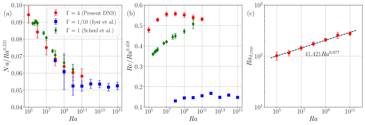
Figure 2(a,b) plot the Nusselt and Reynolds numbers, and versus the Rayleigh number , compensated by the high- scaling result of Iyer et al. (2020); here . We also compare our results with those of Scheel and Schumacher (2017) in a closed cylinder at . While the Nusselt numbers collapse fairly well (figure 2(a)) and are in agreement with previous simulations for similar parameters and those for from van Reeuwijk et al. (2008), the Reynolds number shows a strong geometry dependence (figure 2(b)): they show good agreement in scaling exponents at high but not in the prefactor. Figure 2(c) shows the thermal fluctuation boundary layer thickness-based Rayleigh number versus , together with the power law fit. Statistics in the all runs are obtained for more than 100 free-fall times ; see table 1. We also verified that the vertical profiles of the temperature fluctuation, fitted by polynomial orders and 9 at and and 9 at , collapse on each other. These observations confirm that the DNS are sufficiently well-resolved.
| 5 | 71 | 1000 | ||||||
| 7 | 57 | 1000 | ||||||
| 9 | 42 | 1000 | ||||||
| 7 | 24 | 1000 | ||||||
| 9 | 16 | 400 | ||||||
| 9 | 13 | 200 | ||||||
| 5 | 11 | 100 |
III Mean temperature and velocity profiles
The mean velocity profiles for the horizontal components are obtained by a combined average over the area and statistically independent realizations of the turbulent flow separated from each other by at least 5 as
| (2) |
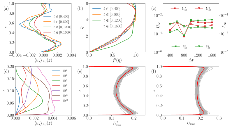
for . Figure 3 displays the result of this analysis for . In panel (a), the mean profile of the -velocity component is shown as a function of the averaging time which was varied from (= 20 snapshots) to (= 80 snapshots). The profile converges steadily to zero, though not uniformly. A fit of the mean profiles to the two-dimensional Blasius solution has been applied subsequently; the solution and (Schlichting and Gersten, 2016). Here, is the stream function and and . Recall that at distance the Blasius profile reaches a streamwise velocity magnitude of .
In the absence of a definable leading edge distance , we match and to which is reported in panels (b,c) of figure 3. Therefore, the numerical profiles are rescaled such that the first local maximum of corresponds to . The fits are shown again for different time intervals. It is seen in panel (c) that the velocity scale drops to a very small magnitude while in case of . In table 2, the results for all Rayleigh numbers and both horizontal components are listed. No clear trend of the velocity with Rayleigh number is detectable, the magnitude is between and . The boundary layer thickness parameters vary as well when - and -directions are compared at fixed . They decrease with increasing Rayleigh number. Furthermore, we calculate the corresponding shear Reynolds numbers , which are found to be very small for all cases. We have also repeated this analysis for a combination of both components (not shown), though not for the magnitude which would become insensitive to different directions of local flow patterns. Panel (d) of figure 3 shows the mean profiles for all 7 simulation runs.
Panels (e) and (f) show the vertical profiles of root-mean-square velocities in red,
| (3) |
together with profiles obtained in the individual snapshots in gray.
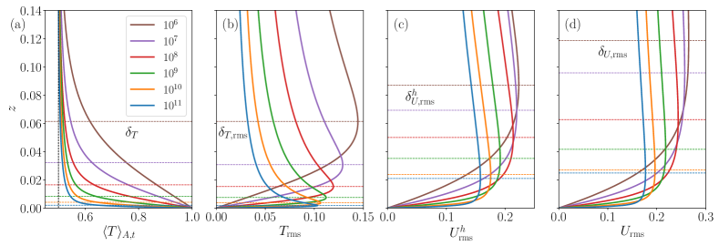
Figure 4 summarizes mean profiles for all 7 simulation runs, the mean temperature profile and the root-mean-square profiles of temperature, horizontal velocity components, and all three velocity components. The temperature fluctuation profile is obtained by with . The correspondingly related characteristic scales are indicated by horizontal dashed lines and detailed in table 3. It is seen that the thermal boundary layer thickness is slightly larger than the distance from the wall of the maximum of the temperature fluctuation profile, . Increasingly larger are distances from the wall to the maxima of the velocity fluctuation profiles, obeying a ratio of for up to approximately 14 for ; see panel (d).
| ( | ( | ( | ( | |
| ( | ( | ( | ( | |
| ( | ( | ( | ( | |
| ( | ( | ( | ( | |
| ( | ( | ( | ( | |
| ( | ( | ( | ( | |
| ( | ( | ( | ( |
IV Scaling laws of fluctuations with Rayleigh number
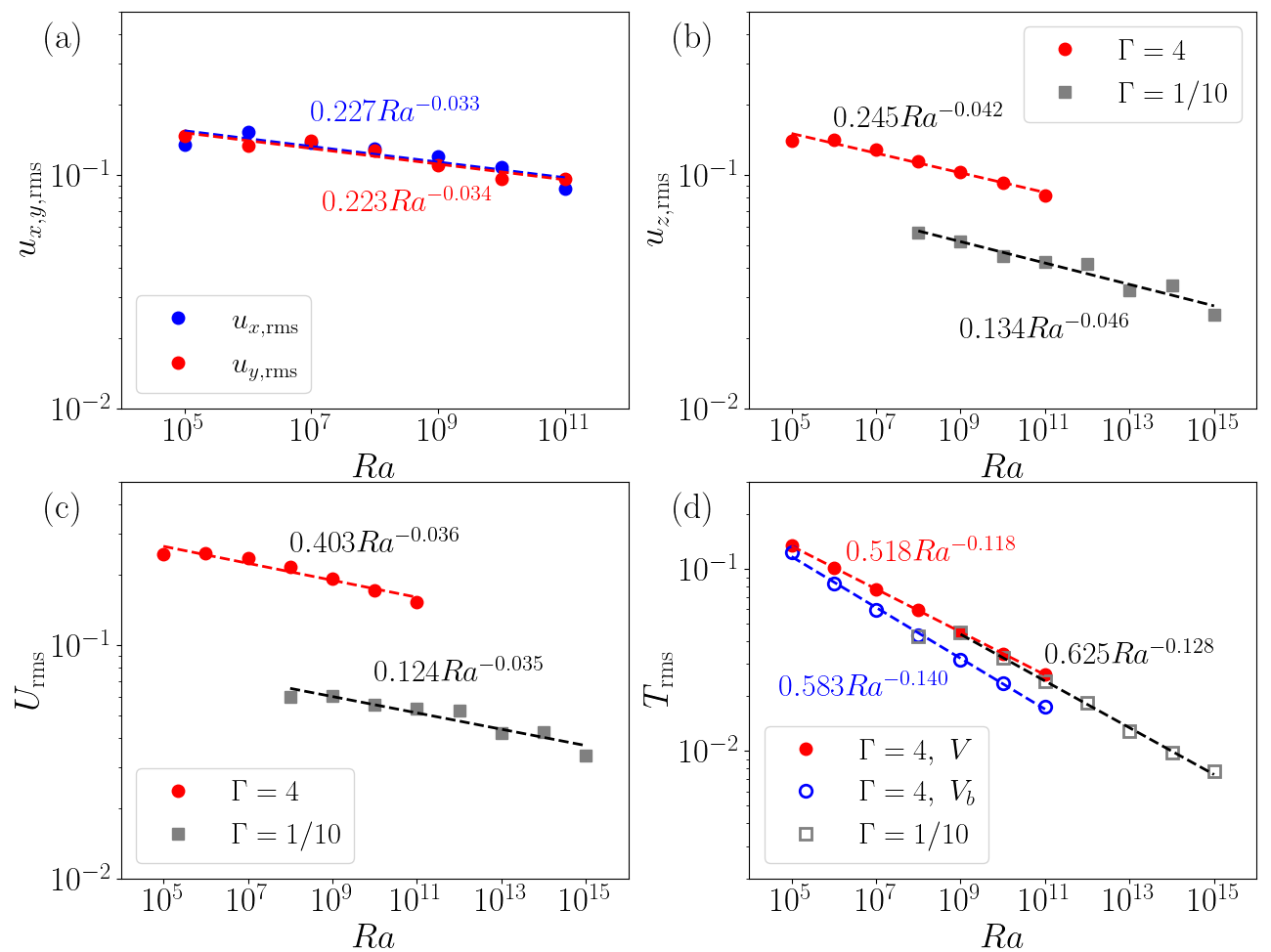
Figure 5 summarizes the root-mean-square fluctuations of the three velocity components and the temperature. They are obtained by a combined average with respect to the full volume and time, e.g. . The quantity denotes again the fluctuations with respect to all three velocity components. It is seen that the dependence of the velocity fluctuations on the Rayleigh number is very weak with . The temperature fluctuations drop with a smaller power law exponent, , which is found to be for the present data. This exponent is slightly smaller in magnitude than those reported in experiments in cylindrical cells of aspect ratio 1/2. For comparison, Castaing et al. (1989), Niemela et al. (2000) and Wu and Libchaber (1992) report exponents of . We also analysed the temperature fluctuations in the bulk of the layer, which takes a volume average with respect to and time. The exponent changes to which is closer to the experiments. We have verified that a variation of the thickness of the bulk volume does not alter the results significantly.
In panels (b–d) of figure 5, we added data from the DNS of Iyer et al. (2020) for comparison, which were obtained in a closed slender cylindrical cell of aspect ratio . It is seen that exponents of the power law fits are close to those of the present simulation series. The prefactors differ as expected, because the former DNS data were obtained for a geometrically constrained convection flow. This finding of nearly the same scaling exponents suggests a robust geometry-independent trend of all fluctuations with respect to the Rayleigh number. Geometry-specific aspects mostly affect the prefactor.
V Decomposition into coherent and incoherent boundary layer regions
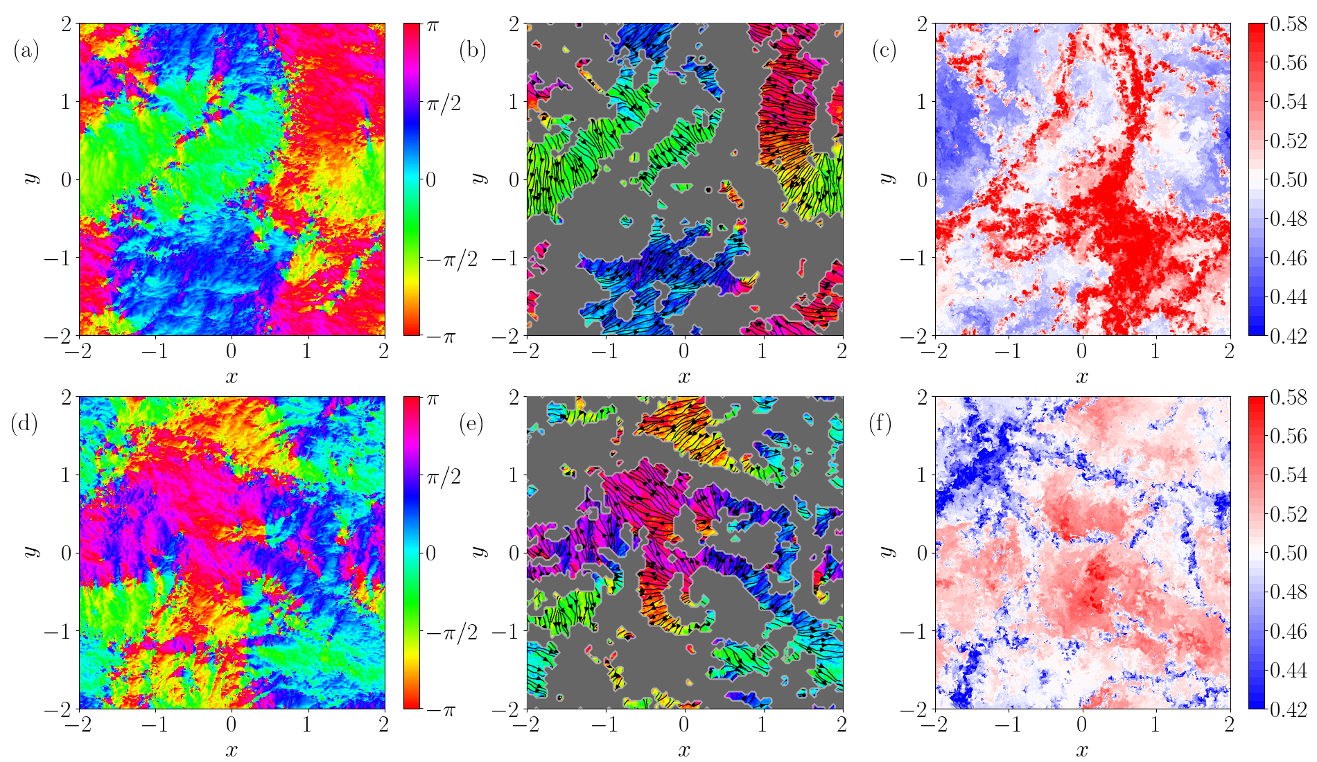
The orientation of the boundary layer flow varies strongly as shown in figures 6 (a) and (d), where we plot the pointwise orientation angle of the horizontal velocity for a snapshot at at and , respectively. At both these heights, we break down the horizontal plane into a cover of disjoint square boxes of area content , where . We then calculate the mean horizontal velocity in each of the and decompose the cross section into coherent and incoherent boundary layer regions for and , respectively. Panels (b, e) of figure 6 show that coherent shear-dominated patches separated by incoherent flow regions (in gray). The superposed streamlines indicate the different flow orientations of the shear-dominated regions. Panels (c,f) show the corresponding snapshots of the temperature field at above the bottom and below the top which is a distance of 25 away from the walls.
It is clearly seen that the hotter regions at and the colder regions at coincide with the incoherent flow regions at the edge of the thermal boundary layer. This is the imprint of the turbulent superstructure of convection in this setup at . We have also determined that the area fraction of the incoherent regions remains nearly constant at approximately 60% of for the whole Rayleigh number range, which further supports its connection to the turbulent superstructure that consists of a few large-scale circulation rolls which extend over the periodic horizontal boundaries. The physical interpretation is that the incoherent regions correspond to the upwelling (downwelling) motion of clustered plumes outside shear dominated patches. It suggests a vertical coarsening from the plate into the bulk, which remains to be analysed in the future.
VI Conclusions
Our DNS of the turbulent Rayleigh-Bénard convection encompasses a Cartesian domain with and periodic boundary conditions in the horizontal directions. These simulations up to are aimed at being close to the original canonical case of a plane convection layer between a pair of infinitely extended rigid plates. We demonstrated that a standard mean flow analysis with a subsequent match to laminar boundary layer profiles gives no systematic profiles; to the extent that we can define them, they are very small in shear Reynolds numbers. In the long-time limit, which we could follow for 1600 at , the velocity mean profiles have to converge to due to homogeneity in and . The simulations by Hartlep et al. (2003) (for ) also found that the mean flow contained very little energy, but De et al. (2018) found a long time periodicity to the mean flow for .
Rather than having a mean flow profile with small fluctuations, we are faced with small mean velocity amplitudes with fluctuations that are up to 3 orders of magnitude larger when the statistics are taken over finite time intervals , as seen from comparisons of table 2 with the data in figure 4. The strong fluctuations cause the boundary layer thickness scales of temperature and velocity to differ by an order of magnitude for the highest Rayleigh numbers, as summarized in table 3. These results hold for all Rayleigh numbers of the series, but become particularly pronounced for , a range to which most previous larger-aspect-ratio DNS studies did not advance.
Our analysis also revealed that the velocity boundary layer in the present configuration is a carpet of differently oriented shear dominated patches interspersed by regions of incoherent mean flow, the latter of which occupies about 60% of the plate area for all Rayleigh numbers. This heterogeneous composition crystallizes particularly for , underlying again the importance of DNS with larger aspect ratios and high Rayleigh numbers. The present results also raise many questions on the possible transition mechanisms of the boundary layer to a turbulent regime and the possible consequences for the global heat transfer. The heterogeneity of the velocity boundary layer detected here suggests to us the prevalence of local, rather than global, instability mechanisms, which would bring us back to the marginal stability concept of the boundary layer, see e.g. Howard (1966). However, figure 2(c) shows a power law fit of with a very small exponent and . The resulting are by at least a factor of 4 smaller than Howard’s critical Rayleigh number of . These open points will form the subject of further studies including higher Rayleigh numbers in this configuration.
Acknowledgements.
The work of RJS is funded by the European Union (ERC, MesoComp, 101052786). Views and opinions expressed are however those of the authors only and do not necessarily reflect those of the European Union or the European Research Council. The work of JDS was supported by a Mercator Fellowship of the Deutsche Forschungsgemeinschaft within the Priority Programme DFG-SPP 1881 on Turbulent Superstructures. The authors gratefully acknowledge the Gauss Centre for Supercomputing e.V. (https://www.gauss-centre.eu) for funding this project by providing computing time through the John von Neumann Institute for Computing (NIC) on the GCS Supercomputer JUWELS at Jülich Supercomputing Centre (JSC).References
- Ahlers et al. [2009a] G. Ahlers, S. Grossmann, and D. Lohse. Heat transfer and large scale dynamics in turbulent Rayleigh-Bénard convection. Rev. Mod. Phys., 81(2):503–537, April 2009a.
- Ahlers et al. [2009b] Guenter Ahlers, Eberhard Bodenschatz, Denis Funfschilling, and J. Hogg. Turbulent Rayleigh-Bénard convection for a Prandtl number of 0.67. J. Fluid Mech., 641:157–167, November 2009b.
- Castaing et al. [1989] B. Castaing, G. Gunaratne, F. Heslot, L. P. Kadanoff, A. Libchaber, S. Thomae, X.-Z. Wu, S. Zaleski, and G. Zanetti. Scaling of hard thermal turbulence in Rayleigh-Bénard convection. J. Fluid Mech., 204:1–30, July 1989.
- Chavanne et al. [1997] X. Chavanne, F. Chillà, Bernard Castaing, B. Hebral, B. Chabaud, and J. Chaussy. Observation of the ultimate regime in Rayleigh-Bénard convection. Phys. Rev. Lett., 79(19):3648–3651, 1997.
- Chillà and Schumacher [2012] F. Chillà and J. Schumacher. New perspectives in turbulent Rayleigh-Bénard convection. Eur. Phys. J. E, 35(7):58, 2012.
- Creyssels and Martinard [2024] M. Creyssels and D. Martinard. Stability analysis of sheared thermal boundary layers and its implication for modelling turbulent Rayleigh-Bénard convection. Eur. J. Mech. B/Fluids, 105:97–103, 2024.
- De et al. [2018] A. K. De, V. Eswaran, and P. K. Mishra. Dynamics of plumes in turbulent Rayleigh–Bénard convection. Eur. J. Mech. B/Fluids, 72:164–178, 2018. doi: 10.1016/j.euromechflu.2018.05.007.
- Fischer et al. [2022] P. F. Fischer, S. Kerkemeier, M. Min, Y.-H. Lan, M. Phillips, T. Rathnayake, E. Merzari, A. Tomboulides, A. Karakus, N. Chalmers, and T. Warburton. NekRS, a GPU-accelerated spectral element Navier–Stokes solver. Parallel Comput., 114:102982, 2022.
- Hartlep et al. [2003] T. Hartlep, A. Tilgner, and F.H. Busse. Large scale structures in Rayleigh-Bénard convection at high Rayleigh numbers. Phys. Rev. Lett, 91:064501, 2003. doi: 10.1103/PhysRevLett.91.064501.
- Howard [1966] L. N. Howard. Convection at high Rayleigh number. Applied Mechanics, 11th Congress of Applied Mechanics, Munich, pages 1109–1115, 1966.
- Iyer et al. [2020] K. P. Iyer, J. D. Scheel, J. Schumacher, and K. R. Sreenivasan. Classical 1/3 scaling of convection holds up to Ra=. Proc. Natl. Acad. Sci. U.S.A., 117:7594–7598, February 2020.
- Kadanoff [2001] L. P. Kadanoff. Turbulent heat flow: Structures and scaling. Phys. Today, 54(8):34–39, August 2001.
- Kerr [1996] R. M Kerr. Rayleigh number scaling in numerical convection. J. Fluid Mech., 310:139–179, January 1996.
- Lindborg [2023] E. Lindborg. Scaling in Rayleigh-Bénard convection. J. Fluid Mech., 956:A34, 2023.
- Niemela et al. [2000] J. J. Niemela, L. Skrbek, K. R. Sreenivasan, and R. J. Donnelly. Turbulent convection at very high Rayleigh numbers. Nature, 404:837–840, January 2000.
- Pandey et al. [2018] A. Pandey, J. D. Scheel, and J. Schumacher. Turbulent superstructures in Rayleigh-Bénard convection. Nat. Commun., 9:2118, May 2018.
- Rayleigh [1916] O. M. Lord Rayleigh. LIX. On convection currents in a horizontal layer of fluid, when the higher temperature is on the under side. Philos. Mag., 32:529–546, 1916.
- Scheel and Schumacher [2017] J. D. Scheel and J. Schumacher. Predicting transition ranges to fully turbulent viscous boundary layers in low Prandtl number convection flows. Phys. Rev. Fluids, 2(12):123501, December 2017.
- Schlichting and Gersten [2016] H. Schlichting and K. Gersten. Boundary-layer theory. Springer Berlin, Heidelberg, 2016.
- Shi et al. [2012] N. Shi, M. S. Emran, and J. Schumacher. Boundary layer structure in turbulent Rayleigh–Bénard convection. J. Fluid Mech., 706:5–33, June 2012.
- Shishkina and Lohse [2023] O. Shishkina and D. Lohse. Ultimate turbulent thermal convection. Phys. Today, 76:26–32, 2023.
- Sreenivasan et al. [2002] K. R. Sreenivasan, A. Bershadskii, and J. J. Niemela. Mean wind and its reversal in thermal convection. Phys. Rev. E, 65:056306, 2002.
- Stevens et al. [2011] R. J. A. M. Stevens, D. Lohse, and R. Verzicco. Prandtl and Rayleigh number dependence of heat transport in high Rayleigh number thermal convection. J. Fluid Mech., 688:31–43, 2011.
- Urban et al. [2012] P. Urban, P. Hanzelka, T Kralik, V. Musilová, A Srnka, and Ladislav Skrbek. Effect of Boundary Layers Asymmetry on Heat Transfer Efficiency in Turbulent Rayleigh-Bernard Convection at Very High Rayleigh Numbers. Phys. Rev. Lett., 109(15):154301, October 2012.
- van Reeuwijk and Jonker [2008] M. van Reeuwijk and H. J. J. Jonker. Wind and boundary layers in Rayleigh-Bénard convection. II. Boundary layer character and scaling. Phys. Rev. E, 77:036312, 2008.
- van Reeuwijk et al. [2008] M. van Reeuwijk, H. J. J. Jonker, and K. Hanjalic. Wind and boundary layers in Rayleigh-Bénard convection. I. Analysis and modeling. Phys. Rev. E, 77(3):036311, 2008.
- Verma [2018] M. K. Verma. Physics of Buoyant Flows: From Instabilities to Turbulence. World Scientific, Singapore, 2018.
- Wu and Libchaber [1992] X. Z. Wu and A. Libchaber. Scaling relations in thermal turbulence: The aspect ratio dependence. Phys. Rev. A, 45:842–845, 1992.